Adaptive Hybrid Simulations for Multiscale Stochastic Reaction Networks

Abstract

The probability distribution describing the state of a Stochastic Reaction Network evolves according to the Chemical Master Equation (CME). It is common to estimated its solution using Monte Carlo methods such as the Stochastic Simulation Algorithm (SSA). In many cases these simulations can take an impractical amount of computational time. Therefore many methods have been developed that approximate the Stochastic Process underlying the Chemical Master Equation. Prominent strategies are Hybrid Models that regard the firing of some reaction channels as being continuous and applying the quasi-stationary assumption to approximate the dynamics of fast subnetworks. However as the dynamics of a Stochastic Reaction Network changes with time these approximations might have to be adapted during the simulation. We develop a method that approximates the solution of a CME by automatically partitioning the reaction dynamics into discrete/continuous components and applying the quasi-stationary assumption on identifiable fast subnetworks. Our method does not require user intervention and it adapts to exploit the changing timescale separation between reactions and/or changing magnitudes of copy numbers of constituent species. We demonstrate the efficiency of the proposed method by considering examples from Systems Biology and showing that very good approximations to the exact probability distributions can be achieved in significantly less computational time.

I Introduction

Chemical reaction networks, where a finite number of molecular species interact with each other through a fixed number of reaction channels, are an important tool for modeling many biochemical systems. The reaction dynamics is invariably noisy due to the discrete nature of molecular interactions which causes the timing of reactions to be random. It is known that this noise can be neglected for systems with high copy-numbers of all the species, and the dynamics can be modeled deterministically through a set of ordinary differential equations goutsias2007classical . However many biological systems involve molecular species with low copy-numbers and hence the randomness in the dynamics can have a significant impact on the properties of the system. This has been demonstrated in a number of biological systems, such as gene expression mcadams1997stochastic , piliation of bacteria munsky2005stochastic and polarization of cells fange2006noise , as well as in synthetic biological circuits such as the Toggle Switch Gardner2000 and the Repressilator elowitz2000synthetic .

To understand the role of noise and its effects, reaction networks are commonly modeled as stochastic processes with Markovian dynamics where the state represents the copy-numbers of the molecular species goutsias2013markovian . The dynamics of the distribution of a Markov process representing the reaction network evolves according to the Chemical Master Equation (CME) which is a set of ordinary differential equations (1). The size of this system is equal to the number of elements in the state space, which is typically infinite, making the task of solving the CME practically impossible for most interesting systems. One can solve a projection of the CME onto a finite subspace, but this only works for small systems munsky2006finite . Other methods are developed that allow the direct solution of the CME for specific classes of networks Kazeev2014 .

If the CME cannot be solved directly, one usually resorts to Monte Carlo methods to generate trajectories of the underlying stochastic process and approximate the probability distribution through a large number of simulations. These simulations can be performed using Gillespie’s Stochastic Simulation Algorithm (SSA) or its variants gillespie2007stochastic , that generate exact sample paths by taking into account the firing of each reaction within the simulation time-period. Several biological systems have reactions spanning a wide range of timescales, either due to variation in the magnitude of the rate constants or variations in the copy-numbers of the constituent species. If the system has reactions with fast timescales, then simulation schemes like SSA can take an impractical amount of time E2005 ; Cao2005 .

To handle this problem, approximate schemes such as $\tau$-leaping methods have been developed, that perform multiple reactions at each step gillespie2001approximate . Such methods are very efficient in simulating many systems with high reaction rates and many enhancements have been proposed to automatically select a proper leap-size cao2006efficient ; cao2007adaptive or deal with networks where the dynamics is “stiff” and some reactions occur on a very fast timescale rathinam2003stiffness .

In most biological applications, one is interested in computing the probability distributions described by a CME. If we can capture the necessary stochasticity using approximate sample paths that are easier to simulate, then we can efficiently obtain a close approximation to the solution of a CME. For this to work we need to identify and conserve the important sources of stochasticity while discarding the insignificant stochastic effects. The dynamical law of large numbers suggests that stochastic effects are less important for a species if the copy-numbers are large kurtz1978strong . For example, consider a simple gene-expression network, where DNA is transcribed into mRNA and mRNA is translated into proteins. One might expect that the stochasticity of transcription and translation of low copy-number DNA and mRNA can be important but the stochasticity of the high-copy number proteins for downstream processes to be unimportant. If the copy-numbers of all the species are large, then under a suitable scaling of rate constants, the process describing the species concentrations , converges in the limit of infinite copy-numbers to the reaction rate equations that correspond to the deterministic model of the reaction network kurtz1978strong . Instead of scaling the copy-numbers of all the species uniformly and taking the limit, one can construct processes where the species are partitioned into a set described by concentrations and a set described by copy-numbers. Such a process has been shown to converge in the infinite copy-number limit for a number of examples kang2013separation ; crudu2009hybrid . The limiting processes in these cases are hybrid processes, that combine both deterministic and Markovian dynamics and, can be called Piecewise Deterministic Markov processes (PDMP) davis1984piecewise .

This idea has been exploited in various hybrid schemes haseltine2002approximate ; Pahle2002 ; Neogi2004 ; Bentele2005 ; salis2005accurate ; crudu2012convergence ; alfonsi2005 ; Hoops2006 ; Griffith2006 ; Puchaka2004a ; Burrage2004a ; Harris2006 , which mostly differ in the way that the partitioning is performed and the way in which the hybrid system is simulated. The partitioning of the species and/or reactions is either done manually or certain threshold-values are chosen for different properties of the system, e.g. the copy-numbers of species Neogi2004 ; Pahle2002 ; Hoops2006 , the propensities of reactions haseltine2002approximate ; Harris2006 , the approximated copy-number fluctuations of species Bentele2005 or a combination of species copy-numbers and reaction propensities salis2005accurate ; alfonsi2005 ; Griffith2006 ; Burrage2004a ; Puchaka2004a . For the simulation, various combinations of SSA, $\tau$-leaping, stochastic differential equations (SDE) and ordinary differential equations (ODE) are possible. Most methods combine the SSA approach with a SDE or an ODE approach haseltine2002approximate ; salis2005accurate ; Griffith2006 ; alfonsi2005 ; Pahle2002 ; Hoops2006 but there are also methods that introduce a regime for $\tau$-leaping Puchaka2004a ; Burrage2004a ; Harris2006 . Another important point for the simulation is the way in which the timings of discrete events is approximated. When integrating the system with $\tau$-leaping, SDE or ODE approach, the propensities of the discrete reactions change with time. Incorporating these time-dependent propensities into the sampling of the discrete event times improves the accuracy of these methods. As soon as the criteria for the partitioning of the system is defined, one can establish an adaptive scheme to repartition the system when necessary. This is important for situations where the orders of magnitudes of the species copy-numbers change significantly over time, a feature found in many important reaction networks from Systems Biology such as transcriptional bursting in gene expression chubb2006transcriptional or the synthetic Repressilator circuit elowitz2000synthetic . How to properly decide when a repartitioning is necessary remains an open issue. We refer the reader to pahle2009biochemical_b for a more comprehensive overview.

The dynamical law of large numbers can be exploited to approximate the dynamics when reaction timescales differ due to variations in the copy-numbers of the constituent species. As mentioned before, timescale separation between reactions can also be caused due to differences in the magnitudes of the rate constants Cao2005 . Some hybrid schemes simplify the dynamics in this situation by applying the quasi-stationary assumption for the dynamics of fast subnetworks crudu2012convergence . This approach is justified in situations where the exact dynamical details of fast subnetworks are unimportant, but only the distributions of the fast species are required to correctly estimate the propensities of the slow reactions. For example, in many biochemical systems the quasi-stationary assumption can be applied to fast subnetworks consisting of enzyme-substrate interactions and exact simulations of the fast dynamics can be avoided, significantly reducing the computational effort Rao2003 ; Cao2005 .

In this paper we propose a new hybrid scheme to estimate solutions of the CME corresponding to a stochastic reaction network, which may exhibit multiple reaction timescales due to variation in both the magnitudes of rate constants and copy-numbers of the constituent species. Our method relies on the rigorous mathematical framework recently provided by Kang et al. kang2013separation to simplify the dynamics for such networks. In this framework they introduce scaling parameters for rate constants as well as species copy-numbers and give formal criteria for convergence to a PDMP. Using Linear Programming we select these scaling parameters to fulfil their criteria and then simulate the limiting PDMP. When the magnitudes of species copy-numbers change significantly, our method adapts itself by recomputing the appropriate scaling parameters and continues the simulation with the corresponding PDMP. In other words, our method dynamically stitches together several PDMPs to account for the variations in the magnitudes of the species copy-numbers, and the resulting variations in the timescales of various reactions. The method can also automatically identify fast subnetworks and apply the correct quasi-stationary assumption whenever possible.

The paper is organized as follows. In Section II we give a mathematical background and introduce the necessary formalism for the rest of the paper. In Section III we elaborate on the algorithm and provide implementation details of our adaptive hybrid scheme. In Section IV we suggest a possible combination of our scheme with $\tau$-leaping schemes. In Section V we compare our adaptive hybrid scheme with SSA and a fixed PDMP scheme (without dynamic repartitioning) for three different examples. We also make a comparison with an existing hybrid scheme (which also dynamically repartitions). Finally, in Section VI we conclude and give an outlook for future work. Additionally, in Appendix A we explain the application of the quasi-stationary assumption and in Appendix B we provide a mathematical justification for the correctness of our adaptive hybrid scheme.

II Mathematical Preliminaries

The goal of this section is to present the relevant mathematical background for this paper. We start by describing how the dynamics of a reaction network can be modeled as a continuous time Markov chain. Such models are called Stochastic Reaction Networks (SRNs) in this paper. We then motivate and describe the multiscale modeling framework of Kang et al. kang2013separation , which explicitly accounts for the variation in reaction timescales by considering both copy-number scales and the differences in magnitudes of rate constants. We also present the limit theorem proved in Kang et al. kang2013separation which shows that under suitable assumptions, the dynamics of the underlying stochastic process is well-approximated by a Piecewise Deterministic Markov Process (PDMP) which can be far easier to simulate than the original dynamics. Finally we end this section with a brief discussion on how the simplified dynamics can be obtained even in situations where the required assumptions for the limit theorem fail. In such cases it is often possible to first apply the quasi-stationary assumption and then use the PDMP approximation as before.

Stochastic Reaction Network (SRN)

Consider a well-stirred chemical system with $n_{S}$ species $\left\{s_{1},\ldots,s_{n_{S}}\right\}$ which interact according to $n_{R}$ reaction channels of the form

$$\sum_{i=1}^{n_{S}}\nu_{ik}s_{i}\longrightarrow\sum_{i=1}^{n_{S}}\nu^{\prime}_{ik}s_{i},\quad k\in\left\{1,\ldots,n_{R}\right\}$$

where $\nu_{ik}$ and $\nu^{\prime}_{ik}$ denote the number of molecules of the $i$-th species that are consumed and produced by the $k$-th reaction. In the stochastic setting, the reaction dynamics can be represented as a continuous time Markov chain, whose state at any time $t$ is just the vector $x=\left(x_{1},\ldots,x_{n_{S}}\right)$ of copy-numbers of all the species. When the state is $x$, the $k$-th reaction occurs after a random time that is exponentially distributed with rate $\lambda^{\prime}_{k}\left(x\right)$, assuming no other reactions occur first. The function $\lambda^{\prime}_{k}$ is called the propensity function for the $k$-th reaction. We assume that the network only consists of elementary reactions and the propensity functions follow mass action kinetics gillespie2009diffusional , as shown in Table 1.

Reaction type	Consumption stoichiometry	Propensity function
Constitutive	$\nu_{k}=0$	$\lambda^{\prime}_{k}\left(x\right)=\kappa^{\prime}_{k}$
Monomolecular	$\nu_{k}=e_{i}$	$\lambda^{\prime}_{k}\left(x\right)=\kappa^{\prime}_{k}x_{i}$
Bimolecular	$\nu_{k}=e_{i}+e_{j}$, $i\neq j$	$\lambda^{\prime}_{k}\left(x\right)=\kappa^{\prime}_{k}x_{i}x_{j}$
Bimolecular	$\nu_{k}=2e_{i}$	$\lambda^{\prime}_{k}\left(x\right)=\frac{1}{2}\kappa^{\prime}_{k}x_{i}(x_{i}-1)$

Table 1: Description of mass action kinetics. Here $e_{i}$ is the $i$-th standard basis vector in $\mathbb{R}^{n_{S}}$.

The CME corresponding to this SRN is given by

$$\frac{dp\left(x,t\right)}{dt}=\sum_{k=1}^{n_{R}}\lambda^{\prime}_{k}\left(x-\xi_{k}\right)p\left(x-\xi_{k},t\right)-\sum_{k=1}^{n_{R}}\lambda^{\prime}_{k}\left(x\right)p\left(x,t\right)$$ (1)

where $\xi_{k}=\nu^{\prime}_{k}-\nu_{k}$, $\nu_{k}=(\nu_{1k},\dots,\nu_{n_{s}k})$ and $\nu^{\prime}_{k}=(\nu^{\prime}_{1k},\dots,\nu^{\prime}_{n_{s}k})$. In this equation, $p\left(x,t\right)$ is the probability $\mathbb{P}\left(X\left(t\right)=x\right)$, where $\left\{X\left(t\right):t\geq 0\right\}$ is the Markov process describing the reaction dynamics. This process satisfies the following random time-change representation ethier2009markov

$$\begin{split}X\left(t\right)=x(0)+\sum_{k=1}^{n_{R}}Y_{k}\left(\int_{0}^{t}\lambda^{\prime}_{k}\left(X(s)\right)ds\right)\xi_{k}\end{split}$$ (2)

where $\left\{Y_{k}:k=1,\ldots,n_{R}\right\}$ is a family of independent unit rate Poisson processes.

In order to understand the behavior of a SRN it is important to compute the distributions that evolve according to the CME. However note that the CME consists of as many equations as the number of elements in the state space of the reaction dynamics, which is typically very large or infinite. This makes CME practically impossible to solve in most cases and therefore its solution is usually estimated using Monte Carlo methods such as Gillespie’s SSA gillespie2007stochastic which generates exact paths of the underlying stochastic dynamics. As mentioned before, many biological networks contain reactions firing in several different timescales, and in such situations these exact Monte Carlo methods can be computationally intractable due to the “stiffness” of the system rathinam2003stiffness . In these cases, it is sometimes possible to approximate the solutions of a CME using a simplified description of the dynamics, which is obtained by preserving the important sources of stochasticity in the dynamics while discarding the rest. One way to obtain such simplified dynamics is to use the multiscale modeling framework of Kang et al. kang2013separation and show that under certain conditions, the orginal dynamics is well-approximated by a PDMP davis1984piecewise which is often much easier to simulate. We now describe this multiscale modeling framework.

Multiscale models of Stochastic Reaction Networks

A multiscale SRN is characterized by reactions firing at many different timescales. This variation in timescales could be both due to variation in copy-number scales as well as variation in the magnitudes of the rate constants. Kang et al. kang2013separation present a framework for separating both these sources of timescale variation, and obtain PDMP approximations of the dynamics under certain conditions. To apply this framework we first select a large positive number $N_{0}$ that reflects the typical copy-number of a species which is considered abundant in the network. Note that the PDMP approximation that we later describe would ignore the stochasticity in copy-numbers of species if they are of order $N_{0}^{\alpha}$ for some $\alpha>0$. Hence the accuracy of this approximation and our method which relies on it, crucially depends on the choice of $N_{0}$.

As an example, consider a gene expression network where the number of genes is usually $1$ or $2$, the number of mRNAs is in the order of tens and the number of proteins is in the order of thousands. To capture the bursting behavior of stochastic gene expression chubb2006transcriptional we want to keep the discreteness of the genes and the mRNAs. However, the discreteness of reaction channels driven by proteins can often be neglected, as the fluctuations of the protein numbers are rather small compared to the total protein number. Thus we want to approximate the number of proteins as a continuous quantity and reaction channels driven by proteins as occurring continuously. For this purpose we can choose $N_{0}=1000$.

From now on, we refer to a quantity as order $1$ (denoted as $O(1)$) if it remains bounded as $N_{0}$ gets larger. Assume that the rate constants $\kappa^{\prime}_{k}$ have different orders of magnitude. For each reaction $k=1,\ldots,n_{R}$ we pick a $\beta_{k}\in\mathbb{R}$, such that $\kappa_{k}=N_{0}^{-\beta_{k}}\kappa^{\prime}_{k}$ is $O(1)$. We can interpret $\beta_{k}$ as the timescale of the $k$-th reaction, when all the reactants have copy-numbers of order one. To account for the variation in the copy-number scales of species we introduce scaling parameters $\alpha_{i}\geq 0$ for $i=1,\ldots,n_{S}$ such that $Z_{i}^{N_{0}}\left(t\right)=N_{0}^{-\alpha_{i}}X_{i}\left(t\right)$ is $O(1)$, at least for $t$ close to $0$. The choice of scaling parameters $\alpha_{i}$-s and $\beta_{k}$-s is not arbitrary as they must satisfy certain conditions that we later describe. In Section III we will present an automatic scheme for selecting these parameters in a suitable way.

Using these scaling parameters $\alpha_{i}$-s and $\beta_{k}$-s, we can derive the scaled process $\{Z^{N_{0}}\left(t\right)=(Z_{1}^{N_{0}}\left(t\right),\ldots,Z_{n_{S}}^{N_{0}}(t)):t\geq 0\}$ from the original process $\{X\left(t\right):t\geq 0\}$. Replacing $N_{0}$ by $N$ we obtain a family of processes $\left\{Z^{N}\left(t\right):t\geq 0\right\}$ parametrized by $N$. If we can show that the process $Z^{N}$ converges in distribution to another process $Z$ as $N\rightarrow\infty$, then for large values of $N_{0}$, $Z_{i}^{N_{0}}\left(t\right)\approx Z_{i}\left(t\right)$ and hence $X_{i}\left(t\right)\approx N_{0}^{\alpha_{i}}Z_{i}\left(t\right)$ for all $i$. This gives us a way to approximate our original process $X$ with another process $Z$ which can be much simpler to simulate. In the classical thermodynamic limit kurtz1978strong , $N_{0}$ is the volume of the system, $\alpha_{i}=1$ for each $i$ and $\beta_{k}=1,0,-1$ depending on whether the $k$-th reaction is constitutive, monomolecular or bimolecular. In this case the limiting process $Z$ corresponds to the deterministic model of the reaction network and its evolution is given by a systems of ODEs called the reaction rate equations. However for many biochemical networks this classical scaling is not suitable, but a general scaling prescribed by $\left(\alpha_{i},\beta_{k}\right)$ can be used. We now present the main convergence result on which our method is based.

Convergence to a PDMP

Under the scaling prescribed by $\left(\alpha_{i},\beta_{k}\right)$, the random time-change representation of the process $\{Z^{N}(t)=(Z_{1}^{N}(t),\ldots,Z_{n_{S}}^{N}(t)):t\geq 0\}$ is given by

$$Z_{i}^{N}(t)=Z_{i}^{N}(0)+N^{-\alpha_{i}}\sum_{k=1}^{n_{R}}Y_{k}\left(\int_{0}^{t}N^{\beta_{k}+\alpha\cdot\nu_{k}}\lambda_{k}^{N}\left(Z^{N}(s)\right)ds\right)\xi_{ik}$$ (3)

where $Z_{i}^{N}(0)=N_{0}^{-\alpha_{i}}X_{i}(0)$ and $\alpha\cdot\nu_{k}$ denotes the dot product of vectors $\alpha=\left(\alpha_{1},\ldots,\alpha_{n_{S}}\right)$ and $\nu_{k}$. The $\lambda_{k}^{N}$-s are defined by

Reaction	$\emptyset\rightarrow\cdots$	$S_{i}\rightarrow\cdots$	$S_{i}+S_{j}\rightarrow\cdots$	$2S_{i}\rightarrow\cdots$
$\lambda_{k}^{N}\left(z\right)$	$\kappa_{k}$	$\kappa_{k}z_{i}$	$\kappa_{k}z_{i}z_{j}$	$\kappa_{k}z_{i}(z_{i}-N^{-\alpha_{i}})$

with $\kappa_{k}=N_{0}^{-\beta_{k}}\kappa^{\prime}_{k}$. In Theorem 4.1. Kang et al. kang2013separation  prove that the process $Z^{N}$ converges to a well-behaved process $Z$ as $N\rightarrow\infty$, if $\left(\alpha_{i},\beta_{k}\right)$ satisfy

$$\alpha_{i}\geq\beta_{k}+\alpha\cdot\nu_{k}\qquad\text{ for each }i,k\text{ with }\xi_{ik}\neq 0.$$ (4)

Moreover the limiting process $Z$ satisfies

$$Z\left(t\right)=x(0)+\sum_{k\in R_{D}}Y_{k}\left(\int_{0}^{t}\lambda_{k}\left(Z(s)\right)ds\right)\xi_{k}+\sum_{k\in R_{C}}\left(\int_{0}^{t}\lambda_{k}\left(Z(s)\right)ds\right)\xi_{k},$$ (5)

where $\left\{Y_{k}:k\in R_{D}\right\}$ is a family of independent unit rate Poisson processes, and reaction subsets $R_{C},R_{D}\subset\left\{1,\ldots,n_{R}\right\}$ are defined by

$$R_{C}= \left\{k:\alpha_{i}=\beta_{k}+\alpha\cdot\nu_{k}>0\ \text{ for all }i\text{ such that }\xi_{ik}\neq 0\right\}\text{ and}$$

$$R_{D}= \left\{k\not\in R_{C}:\alpha_{i}=\beta_{k}+\alpha\cdot\nu_{k}=0\ \text{ for all }i\text{ such that }\xi_{ik}\neq 0\right\}.$$ (6)

The limiting process $Z$ described by (5) is essentially a Piecewise Determinitic Markov Process (PDMP) because a part of the dynamics, given by reactions in $R_{C}$ evolves continuously (as in an ODE), while another part of the dynamics, given by reactions in $R_{D}$ evolves discretely like a jump Markov process similar to our original process $X$. Note that in general $R_{C}\cup R_{D}\neq\left\{1,\ldots,n_{R}\right\}$ and all reactions not in $R_{C}\cup R_{D}$ do not contribute to the dynamics of the limiting process $Z$.

With the scaling parameters $\left(\alpha_{i},\beta_{k}\right)$ we also define subsets of species by

$$S_{C}= \left\{i\in\left\{1,\ldots,n_{S}\right\}:\alpha_{i}>0\right\}$$

$$S_{D}= \left\{1,\ldots,n_{S}\right\}\setminus S_{C}.$$ (7)

The species in $S_{C}$ change due to reactions in $R_{C}$ and therefore they are measured by “concentrations” and evolve continuously, whereas the species in $S_{D}$ will have discrete state values given by their copy-number. The dynamics of the limiting process $Z$ can then be written as

$$Z_{C}\left(t\right) =x_{C}(0)+\sum_{k\in R_{C}}\left(\int_{0}^{t}\lambda_{k}\left(Z(s)\right)ds\right)\xi_{k}$$

$$Z_{D}\left(t\right) =x_{D}(0)+\sum_{k\in R_{D}}Y_{k}\left(\int_{0}^{t}\lambda_{k}\left(Z(s)\right)ds\right)\xi_{k}$$ (8)

where $Z_{C}\left(t\right)$ and $Z_{D}\left(t\right)$ are vectors with entries $Z_{i}\left(t\right)$ for $i\in S_{C}$ and $i\in S_{D}$ respectively. The definitions of $x_{C}(0)$ and $x_{D}(0)$ are similar.

To simulate such a PDMP, the dynamics of the reactions in $R_{C}$ are basically an Ordinary Differential Equation (ODE) and the reactions in $R_{D}$ can modify its vector field at random times. The ODE can be solved with established and efficient ODE solvers and for large propensities of the reactions channels in $R_{C}$, this can be computationally much cheaper than simulating the discrete individual reactions as Gillespie’s SSA gillespie2007stochastic . Therefore the speed enhancements that our method obtains (by simulating a PDMP (5)) in comparison to SSA, is directly proportional to the number of reactions treated continuously. More details on simulating a PDMP are provided in section III.

For the above convergence result to hold, we need to find scaling parameters $\left(\alpha_{i},\beta_{k}\right)$ such that (4) is satisfied. Note that such a choice always exists as we can simply set each $\alpha_{i}$ and $\beta_{k}$ to $0$ to satisfy these contraints. However with such a trivial choice of scaling parameters, the limiting process $Z$ is same as the original process $X$ and hence we do not obtain any computational advantage in simulating the limiting process. In Section III we describe how these parameters can be automatically chosen using Linear Programming in such a way, that the limiting dynamics is computationally much easier to simulate. The key idea is to treat as many reactions continuously as possible without violating the constraints that imply the PDMP convergence result. We also discuss how they can be properly adapted if the copy-number scales of species vary significantly with time.

Applying the quasi-stationary assumption

Consider the situation where certain species have low copy-numbers but their dynamics is affected by reactions with large rate constants $\kappa^{\prime}_{k}$. In this situation, an appropriate copy-number scaling parameter $\alpha_{i}$ for such species would be close to $0$, since copy-numbers are small, while an appropriate rate constant scaling parameter $\beta_{k}$ for these reactions would be strictly positive. As a consequence, for these low-copy species with fast dynamics (or simply fast species), the constraits (4) will fail to hold for scaling parameters $\left(\alpha_{i},\beta_{k}\right)$ that truly represent the dynamics. If we use our automatic parameter selection procedure given in Section III, then all the reactions involved in changing these fast species will have their $\beta_{k}$-s set to a negative or a small positive value even though their rate constants $\kappa^{\prime}_{k}$-s are large. Hence our method will not be able to treat these fast reactions continuously and therefore it will suffer from the same stiffness problems as Gillespie’s SSA Cao2005 .

To remedy this problem we use another result in Kang et al. kang2013separation , which shows that even with such fast species in the network, well-behaved limits can be obtained for certain projections of the process $Z^{N}$. Such projections correspond to “reduced” reaction networks which only consist of those species that satisfy (4). These reduced models can also consist of linear combinations of fast species that satisfy a constraint analogous to (4). To obtain these reduced models along with their limits, one needs to find subnetworks of fast reaction channels where the quasi-stationary assumption can be applied. Assume that we have such a subnetwork whose internal dynamics is much faster than the surrounding dynamics. If the subnetwork dynamics converges to a stationary distribution then we can use this distribution to estimate the propensities of reactions emanating from this subnetwork pelevs2006reduction ; radulescu2008robust ; crudu2012convergence . In this approach we assume that the species influenced by these fast reaction channels are always at stationarity and hence we do not capture their transient dynamics, thereby saving a lot of computational time Rao2003 ; Cao2005 . The application of quasi-stationary approximation is also called averaging in the mathematical literature. We discuss this approach in greater detail in Appendix A.

III Implementation

The aim of this section is to provide full implementation details of our method for approximating the solution of a CME. The presented algorithms compute a single sample path of the dynamics. The solution of a CME at a certain time $t$ can be approximated by generating several sample paths and computing the histogram of the sample-path values at time $t$. We start by introducing the well-known scheme for simulating a PDMP, where the partitioning of reactions/species into discrete/continuous subsets is fixed. We then describe our adaptive hybrid scheme, where this partitioning changes with time due to the variation in the orders of magnitude of species copy-numbers. This partitioning is based on the scaling parameters $\alpha_{i},\beta_{k}$, mentioned before, and we describe how these parameters can be appropriately chosen using Linear Programming. In both these approaches (Fixed and Adaptive PDMP) computational time can be saved by applying the quasi-stationary assumption on fast subnetworks consisting of discrete species and discrete reactions. We explain this procedure and indicate how it can be integrated into our method.

The inputs that are the same to all the algorithms are given by:

$\mathbf{t_{0}}$

initial time of simulation

$\mathbf{t_{f}}$

final time of simulation

$\mathbf{z_{0}}$

initial state vector of simulation

$\nu_{ik}$ for $i\in\left\{1,\ldots,n_{S}\right\}$ and $k\in\left\{1,\ldots,n_{R}\right\}$

the consumption stoichiometries

$\nu^{\prime}_{ik}$ for $i\in\left\{1,\ldots,n_{S}\right\}$ and $k\in\left\{1,\ldots,n_{R}\right\}$

the production stoichiometries

$\kappa^{\prime}_{k}$ for $k\in\left\{1,\ldots,n_{R}\right\}$

the unscaled reaction rate constants

$N_{0}\in\mathbb{N}$

copy-number scale considered to be large (default value $N_{0}=1000$)

The adaptive algorithm needs two additional inputs:

$\mu$

continuous copy-number scale threshold (default value $\mu$ = 0.5)

$\eta$

adaptation scale threshold (default value $\eta=0.9$)

These are described in more detail in the following sections.

We will use the following notation throughout this section:

$\mathbf{P}$

total number of firings considering all discrete reactions occurring from $t_{0}$ until $t_{f}$

$\mathbf{t_{r}(p)}$

time of the $p$-th firing considering all discrete reactions for $p=1,\ldots,P$. We define $t_{r}\left(0\right)=t_{0}$ and $t_{r}\left(P+1\right)=\infty$.

$\mathbf{R_{D}(t})$

the set of discrete reaction channels at time $t$

$\mathbf{R_{C}(t)}$

the set of continuous reaction channels at time $t$

$\mathbf{S_{D}(t})$

the set of discrete species at time $t$

$\mathbf{S_{C}(t)}$

the set of continuous species at time $t$

$\mathbf{z\left(t\right)}$

the state vector at time $t$

Note that the entries in the state vector $z\left(t\right)$ corresponding to $S_{D}\left(t\right)$ are non-negative integers representing the species copy-numbers whereas the entries corresponding to $S_{C}\left(t\right)$ are non-negative real numbers representing the scaled species copy-numbers.

Simulation of Fixed Piecewise Deterministic Markov Processes

Consider a typical PDMP model where the continuous and discrete reaction subsets, given by $R_{C}\left(t\right)$ and $R_{D}\left(t\right)$ respectively, and the induced species partition $S_{C}\left(t\right)$ and $S_{D}\left(t\right)$ do not depend on the time $t$. The usual algorithm to simulate such models is to evolve the part of the model that is described deterministically until the next discrete reaction occurs. When a discrete reaction occurs, the copy-numbers are updated accordingly. This is repeated until the end-timepoint of the simulation is reached. To evolve the deterministic system we use existing ODE solvers.

The time increment $\Delta t_{p}=t_{r}\left(p\right)-t_{r}\left(p-1\right)$ between the $(p-1)$-st and $p$-st reaction is defined by the stopping condition

$$\int_{t_{r}\left(p-1\right)}^{t_{r}\left(p-1\right)+\Delta t_{p}}\sum_{k\in R_{D}}\lambda_{k}\left(z\left(t\right)\right)=u_{p}$$ (9)

where $u_{p}=-\log\left(q_{p}\right)$, $q_{p}\sim\mathcal{U}\left[0,1\right]$ and $\mathcal{U}\left[0,1\right]$ is the uniform distribution over $[0,1]$. At time $t_{r}\left(p\right)$ the $k$-th reaction in $R_{D}$ fires with probability

$$\frac{\lambda_{k}\left(z\left(t_{r}\left(p\right)\right)\right)}{\sum_{m\in R_{D}}\lambda_{m}\left(z\left(t_{r}\left(p\right)\right)\right)}\quad.$$ (10)

For time $t_{r}\left(p-1\right)<t<t_{r}\left(p\right)$, only the states of continuous species will change according to the ordinary differential equation given by

$$\frac{d}{dt}z\left(t\right)=\sum\limits_{k\in R_{C}}\lambda_{k}\left(z\left(t\right)\right)\xi_{k}\quad.$$ (11)

We start the simulation at time $t=t_{0}$ and $z\left(t_{0}\right)=z_{0}$ and generate a random variable $u_{1}$ with distribution $\mathcal{U}\left[0,1\right]$. We evolve the state $z\left(t\right)$ according to (11) until the first discrete reaction occurs at time $t_{r}\left(1\right)=t_{0}+\Delta t_{1}$, defined by (9). We sample the reaction $k$ from $R_{D}$ according to (10) and set $z\left(t_{r}\left(1\right)\right)=z\left(t_{r}\left(1\right)-\right)+\xi_{k}$. These steps are repeated until we reach the final time $t_{f}$. Below we give an algorithmic description of the procedure we just described.

Algorithm 1: Fixed PDMP

1. $t\leftarrow t_{0}$, $z\left(t_{0}\right)\leftarrow z_{0}$, $p\leftarrow 1$

2. while $t<t_{f}$ do

3. % Set up random variable for the stopping condition (9)

4. $u_{p}\leftarrow-\log\left(q_{p}\right)$ where $q_{p}\sim\mathcal{U}\left[0,1\right]$

5. evolve

6. $z$ according to $\frac{d}{dt}z\left(t\right)=\sum\limits_{k\in R_{C}}\lambda_{k}\left(z\left(t\right)\right)\xi_{k}$

7. until $t=t_{f}$ or $t=t_{r}\left(p\right)$ according to (9)

8. if $t=t_{r}\left(p\right)$ then

9. % Determine which discrete reaction occurs at $t$ and
   update state vector

10. Sample $r$ with $\text{Pr}\left(r=k\right)\sim\lambda_{k}\left(z\left(t\right)\right),k\in R_{D}$

11. $z\left(t\right)\leftarrow z\left(t-\right)+\xi_{r}$

12. $p\leftarrow p+1$

13. end if

14. end while

Adaptive Simulation of Piecewise Deterministic Markov Processes

For SRNs that show big variation in copy-numbers over time, it may be impossible to find a fixed partitioning of the reaction and species sets that works well until the final time $t_{f}$. This motivated us to extend the fixed PDMP algorithm into an adaptive scheme, where the partitioning can change with time, depending on the copy-number scales of different species. The general idea is to define bounds for the copy-numbers in a suitable manner and upon leaving these bounds the partitioning of the reaction and species sets is updated according to the current copy-number scales.

The copy-number bounds are defined by parameters $\mu\geq 0$ and $\eta\geq 0$. For a discrete species the upper bound is $N_{0}^{\mu}$, while for a continuous species the lower and upper bounds are $N_{0}^{-\eta}$ and $N_{0}^{\eta}$ respectively. Thus the parameter $\mu$ is used to decide when a species can be considered continuous and the parameter $\eta$ gives the range of re-scaled copy-numbers where no adaptation is performed. We use $\mu=1$ and $\eta=0.9$ as default parameter values. Only in the case of too few or too many adaptations do we advise to try different values for $\eta$. Note that even though the performance of our algorithm depends on the choice of $\mu$ and $\eta$, this dependence is relatively small. For each $i\in\left\{1,\ldots,n_{S}\right\}$ define a set

$$B_{i}^{N_{0}}=\begin{cases}\left[0,N_{0}^{\mu}\right]&\text{ if }i\in S_{D}\\ \left[N_{0}^{-\eta},N_{0}^{\eta}\right]&\text{ if }i\in S_{C}\end{cases}\quad$$ (12)

and update the partitioning of the reactions and species if the value of $x_{i}$ leaves the set $B_{i}^{N_{0}}$.

We implemented our adaptive simulation scheme both with a fixed time step and an adaptive time step. Here we describe the fixed time step algorithm with a time step $dt$: We define a subset $R_{Q}\subseteq R_{D}$ of discrete reactions that influence the continuous dynamics

$$R_{Q}=\left\{k\in R_{D}:\xi_{ik}\neq 0\text{ and }\nu_{il}\neq 0\text{ for some }l\in R_{C}\right\}\quad.$$

After an integration step of the continuous dynamics has been performed, the next time $t_{R}$ of a discrete reaction can be computed by using the sum of discrete propensities $w$ computed in the subroutine integrateStep. This is repeated until either the next discrete reaction time $t_{R}$ would exceed the current time of the integration $t_{N}=t+dt$, or the discrete reaction belongs to $R_{Q}$. If the discrete reaction belongs to $R_{Q}$ then the current time of integration $t_{N}$ is set to the discrete reaction time $t_{R}$.

If the copy-number bounds in relation (12) become invalid, an adaptation procedure is performed where the scaling parameters $\alpha_{i},\beta_{k}$ are recomputed, the state of the system is scaled accordingly and the averaging of fast subnetworks is performed, if possible. The adaptation and averaging procedures are described in more detail in the following sections.

Algorithm 2: Adaptive PDMP

1. $t\leftarrow t_{0}$, $z\leftarrow z_{0}$, $w\leftarrow 0$

2. $u\leftarrow-\log\left(q\right)$ where $q\sim\mathcal{U}\left[0,1\right]$

3. while $t_{0}<t_{f}$ do

4. $t_{N},[z_{N},w_{N}]\leftarrow\text{integrateStep(t, [z, w])}$

5. $\Delta z=0$

6. while $w_{N}\geq u$ do

7. $t_{R}\leftarrow\text{findRoot}(t,w-U,t_{N},w_{N}-U)$

8. [$z_{R},w_{R}]\leftarrow\text{interpolate}(t_{R},t,[z,w],t_{N},[z_{N},w_{N}])$

9. $r\leftarrow k\text{ with probability }p_{k}\propto\lambda_{k}\left(z_{R}+\Delta z\right)$

10. $u\leftarrow u-\log\left(q\right)$ where $q\sim\mathcal{U}\left[0,1\right]$

11. if $r\in R_{Q}$ then

12. $z_{R}\leftarrow z_{R}+\xi_{r}$

13. $t_{N}\leftarrow t_{R}$, $z_{N}\leftarrow z_{R}$

14. Goto step 21

15. else

16. $\Delta z\leftarrow\Delta z+\xi_{r}$

17. $t\leftarrow t_{R}$, $z\leftarrow z_{R}$

18. $w_{N}\leftarrow w_{R}+\sum\limits_{k\in R_{D}}\lambda_{k}(z_{R}+\Delta z)\times(t_{N}-t_{R})$

19. end if

20. end while

21. $t\leftarrow t_{N}$, $z\leftarrow z_{N}+\Delta z$, $w\leftarrow w_{N}$

22. for each $i\in S_{D}\cup S_{C}$ do

23. if $z_{i}$ violates (12)

24. Perform adaptation (Algorithm 3)

25. Goto step 3

26. end if

27. end for

28. end while

Computation of scaling parameters

Our method relies on computing the PDMP approximation based on the framework by Kang et al.kang2013separation  described before. For this we need to pick the scaling parameters $\alpha_{i}$-s and $\beta_{k}$-s such that the PDMP approximation is justified. Moreover, to enhance the computational efficiency, we would also like to maximize the number of reactions that can be treated continuously. We achieve these two objectives by formulating the conditions given by (4) as constraints of a linear program that maximizes a suitably chosen weighted sum of the $\alpha_{i}$-s and $\beta_{k}$-s. Once these parameters have been chosen, the result of Kang et al.kang2013separation  shows that the PDMP approximation must be partitioned according to (II). However such a strict partitioning scheme is often inappropriate from the standpoint of numerical simulations, because the $\alpha_{i}$-s and $\beta_{k}$-s are real numbers. Hence we relax this partitioning criteria by introducing another parameter $\delta$ (with $\delta=1$ as the default value) which decides when a reaction is considered continuous or discrete. Formally, we define

$$R_{C}\left(t\right)=\{k:\alpha_{i}>\delta\ \forall i\text{ s.t. }\xi_{ik}\neq 0\}\quad\text{ and }\quad R_{D}\left(t\right)=\{k:\exists i:\alpha_{i}\leq\delta,\xi_{ik}\neq 0\}.$$ (13)

The partitioning of the species set into discrete and continuous subsets $S_{D}\left(t\right)$ and $S_{C}\left(t\right)$ is defined in Section II.

We now elaborate on the linear program that is solved to find the scaling parameters at time $t$. For each $i\in\left\{1,\ldots,n_{s}\right\}$ let $x_{i}=N_{0}^{\alpha_{i}}z_{i}\left(t\right)$ where the $\alpha_{i}$-s are the scaling parameters before time $t$. For each $i\in\left\{1,\ldots,n_{S}\right\}$ and each $k\in\left\{1,\ldots,n_{R}\right\}$ define

$$A_{i}=\frac{\log(x_{i})}{\log(N_{0})}\quad\text{ and }\quad B_{k}=\frac{\log(\kappa^{\prime}_{k})}{\log(N_{0})}.$$

Here $A_{i}$ gives the copy-number scale of the $i$-th species at time $t$, while $B_{k}$ is a time-independent quantity that gives the natural timescale of the $k$-th reaction, if all its reactant species have copy-numbers of order one. We compute the new scaling parameters by solving the following linear program

$$\begin{array}[]{cc}\operatorname*{maximize}\limits_{\alpha_{i},\beta_{k}}&\psi\sum\limits_{i=1}^{n_{S}}\frac{\alpha_{i}}{A_{i}}+\sum\limits_{i=1}^{n_{R}}\frac{\beta_{k}}{B_{k}}\\ \\ \text{subject to }&0\leq\alpha_{i}\leq A_{i},\beta_{k}\leq B_{k}\quad\forall i,k\\ \text{and }&\alpha_{i}\geq\beta_{k}+\alpha\cdot\nu_{k}\quad\forall i,k\text{ with }\xi_{ik}\neq 0\quad.\end{array}$$ (14)

Essentially we are trying to maximize the values of the scaling parameters $\alpha_{i}$, $\beta_{k}$ such that the constraints (4) are satisfied and $\alpha_{i}$ approximately captures the copy-number scale of the $i$-th species at time $t$ while $\beta_{k}$ approximately captures the natural timescale of the $k$-th reaction. Maximizing these scaling parameters allows us to treat more reactions and species continuously, and therefore enhance the speed of our simulations. We weigh the first term in the objective function by $\psi$ (with $\psi=100$ as the default value) because the correct selection of $\alpha_{i}$-s is more crucial for the partitioning than the $\beta_{k}$-s. We now describe how we automatically adapt the partitioning in our method.

Algorithm 3: Adaptation

1. Solve the linear program (14) to find the $\alpha_{i}$-s and $\beta_{k}$-s

2. Recompute the partitions $R_{C}\left(t\right),R_{D}\left(t\right)$ and $S_{C}\left(t\right),S_{D}\left(t\right)$
   according to (13)

3. Recompute copy-number bounds (12)

4. Optional: Perform averaging (Algorithm 4, see next section)

Averaging of fast subnetworks

After the selection of the scaling parameters in the Adaptation algorithm (Algorithm 3) we try to apply the quasi-stationary assumption on fast subnetworks, if possible. The subnetworks that are suitable for this purpose can be precomputed at the start of the simulation procedure. This can be done for example, by selecting subnetworks based on conservation relationships between species, pseudo-linearity or by checking if a subnetwork is weakly reversible with deficiency zero (see Appendix A). Also, as the number of possible subnetworks grows rapidly with the number of reactions $n_{R}$ in the network, one has to apply some heuristic to limit the search space of subnetworks. A straightforward choice would be to only consider subnetworks with a maximum number of reactions. While implementing the averaging procedure we go through the list of suitable subnetworks that only contain discrete reactions and we compute the timescale-separation $\Delta\zeta\left(R\right)$ as in (15) for all such subnetworks. We select the subnetworks with $\Delta\zeta\left(R\right)\geq\Theta$ and adopt a greedy strategy of repeatedly selecting the largest subnetwork that has not been selected yet. This gives us a list of disjoint subnetworks on which the quasi-stationary assumption can be applied at the current time. Then we compute the first and second moments of the stationary distribution for each selected subnetwork and accordingly update the rate constants of the reactions that connect the subnetwork with the surrounding network. For a description of the implementation details see Appendix A.

IV Combination with $\tau$-leaping

In this section we propose a possible extension of this work by combining $\tau$-leaping schemes with our method to improve its speed or accuracy. Instead of only using two regimes in our simulation, i.e. discrete stochastic jump dynamics and continuous deterministic dynamics, we can add another regime in between where the dynamics is approximated by $\tau$-leaping. To determine which reactions are approximated by $\tau$-leaping and which ones are approximated by continuous deterministic dynamics, the partitioning in (13) can be modified appropriately to introduce a third set of reactions $R_{\tau}$ that are approximated with $\tau$-leaping. The step size $\tau$ of the $\tau$-leap can be computed as described in cao2006efficient :

$$\tau=\min_{i:I}\left\{\frac{\max\left\{\epsilon x_{i}/g_{i},1\right\}}{|\mu_{i}\left(x\right)|},\frac{\max\left\{\epsilon x_{i}/g_{i},1\right\}^{2}}{|\sigma^{2}_{i}\left(x\right)|}\right\},$$

where

$$I=\left\{{i:\xi_{ik}\neq 0\text{ with }k\in R_{\tau}\cup R_{C}}\right\}$$

is the set of species modified by the reactions in $R_{\tau}$ or $R_{C}$. The functions $\mu_{i}\left(x\right)$ and $\sigma_{i}^{2}\left(x\right)$ are given by

$$\mu_{i}\left(x\right)= \sum_{k\in R_{\tau}\cup R_{C}}\xi_{ik}\lambda_{k}\left(x\right)\text{ and }$$

$$\sigma^{2}_{i}\left(x\right)= \sum_{k\in R_{\tau}\cup R_{C}}\xi^{2}_{ik}\lambda_{k}\left(x\right)\quad,$$

where the parameters $\epsilon$ and $g$ are usually taken to be $\epsilon=0.03$ and $g_{i}=3$. It is important to also include the continuous reactions into the step size selection as the leap condition, i.e. the change of reaction propensities during the leap has to be small, might not be satisfied otherwise. Because of our partitioning scheme there is no need to consider reactions involving low-copy number species in a special manner as is done in cao2006efficient by introducing the so-called “critical reactions”. The integration of the continuous dynamics of the system can then be performed with a fixed time step integration scheme where the step size is equal to $\tau$.

V Numerical Examples

In this section we consider three examples from Systems Biology and demonstrate that our adaptive hybrid scheme accurately captures the solution of a CME, and it can outperform the standard SSA and fixed PDMP schemes. In one of the examples we also compare our scheme to an existing adaptive PDMP method by Alfonsi et al. alfonsi2005 .

The first example (Fast Dimerization) illustrates the usefulness of the averaging procedure. In this example partitioning of reactions and species is not required and our scheme reduces to the slow-scale SSA given in Cao et al.Cao2005 . However, the advantage of our method is that the quasi-stationary assumption is applied automatically without any need for explicit computations of the stationary distributions.

The second example (Toggle Switch) shows the performance improvements of PDMP schemes over SSA. In this example there exists a partitioning of the reactions and the species that is valid for the whole simulation period. Our method automatically chooses an appropriate partitioning, without the need for preceding manual analysis of the network, unlike other existing PDMP schemes. We also show results of the method proposed by Alfonsi et al.alfonsi2005 . Note that we implemented this method in an adaptive fashion analogous to our approach and used the same ODE solver (i.e. the Dormand-Prince 5 stepper from the boost odeint library) for the continuous dynamics.

Finally, the third example (Repressilator) demonstrates the advantages of using an Adaptive PDMP scheme for networks that exhibit large variations in the copy-numbers of their species. In this example a fixed partitioning will not work and hence our adaptive method will outperform any fixed PDMP approach in terms of computational efficiency and accuracy.

All simulations were run in parallel on a grid using $128$ cores and using the parameter values for our algorithm given in Table 2. A comparison of the runtimes for each example is given in Figure 1.

$N_{0}$	$\delta$	$\mu$	$\eta$	$\Theta$
$1000$	$1.0$	$1.0$	$0.9$	$0.5$

Table 2: Parameters values used for all examples.

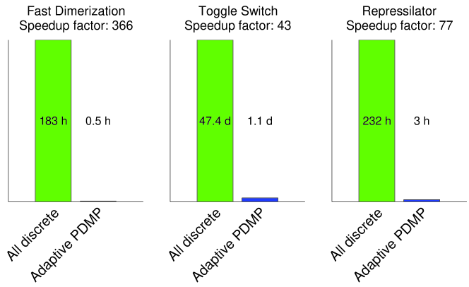
Figure 1: Runtime comparison of fully discrete dynamics and our Adaptive PDMP method. Shown is the comparison of total CPU time required for 100’000 sample paths.

V.1 Fast Dimerization

The fast dimerization SRN Cao2005 consists of $n_{S}=3$ species $s_{0}$, $s_{1}$ and $s_{2}$ and $n_{R}=4$ reactions and is depicted in Figure 2. The reactions are listed in Table 3.

Reaction	$\kappa^{\prime}$	Reaction	$\kappa^{\prime}$
$s_{0}+s_{0}\rightarrow s_{1}$	$1.0$	$s_{1}\rightarrow s_{0}+s_{0}$	$200.0$
$s_{0}\rightarrow\emptyset$	$0.02$	$s_{1}\rightarrow s_{2}$	$0.004$

Table 3: Reactions of the Fast Dimerization network

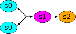
Figure 2: Cartoon of the Fast Dimerization network

The simulation is run from $t_{0}=0$ until $t_{f}=400$ and the initial state is set to $x\left(t_{0}\right)=x_{0}=\left(540,730,0\right)$. Considering the difference in the orders of magnitude of the rate constants for reaction $s_{0}+s_{0}\rightarrow s_{1}$ and $s_{1}\rightarrow s_{0}+s_{0}$ compared to the rate constants for reaction $s_{0}\rightarrow\emptyset$ and $s_{1}\rightarrow s_{2}$, it seems plausible that the dynamics of a subnetwork consisting of the species $s_{0}$ and $s_{1}$ can be averaged. Indeed our adaptive scheme identifies the subnetwork consisting of species $s_{0}$ and $s_{1}$ as suitable for averaging, and using the strategy for zero-deficiency networks the quasi-stationary assumption can be applied. This can be clearly seen in Figure 3, where the copy-numbers of species $s_{0}$ and $s_{1}$ show strong fluctuations for the SSA simulations and only weak fluctuations for the Adaptive PDMP simulations (the weak fluctuations are due to the reaction $s_{1}\rightarrow s_{2}$ which is still simulated with discrete dynamics). The averaging provides a huge performance gain without losing any essential information about the dynamics of the species $s_{2}$.

The simulation of $100^{\prime}000$ sample paths with SSA took a total CPU time of $\approx 183\text{ hours}$. The simulation of $100^{\prime}000$ sample paths with our Adaptive PDMP scheme using zero-deficiency averaging took a total CPU time of $\approx 0.5\text{ hours}$. Figure 3 shows the results of these simulations. The distribution given by the CME (estimated with SSA) closely matches the distribution estimated with our Adaptive PDMP scheme at time $t=200$ (see Figure 4). The Kolmogorov-Smirnov distance between the two distributions is $d_{KS}=0.01$.

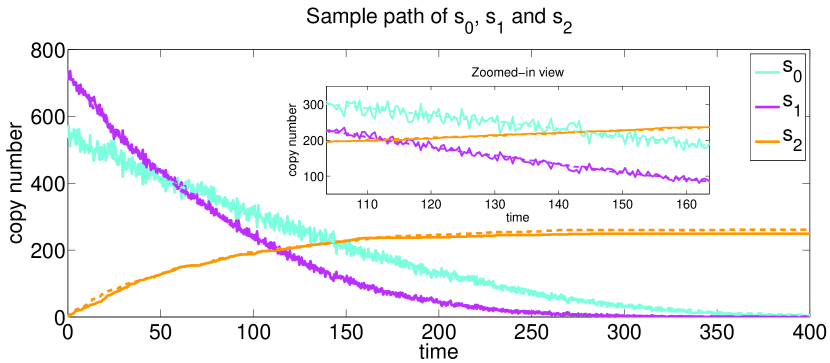
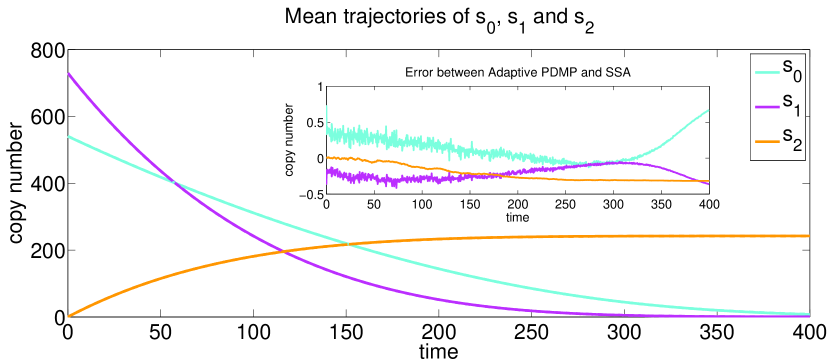
Figure 3: Simulation results of the Fast Dimerization SRN

The upper plot shows a sample path of species $s_{0}$, $s_{1}$ and $s_{2}$ with SSA (solid lines) and with our Adaptive PDMP scheme (dashed lines). The lower plot shows the mean copy-number of species $s_{0}$, $s_{1}$ and $s_{2}$ of $100^{\prime}000$ simulations with SSA and our Adaptive PDMP scheme.

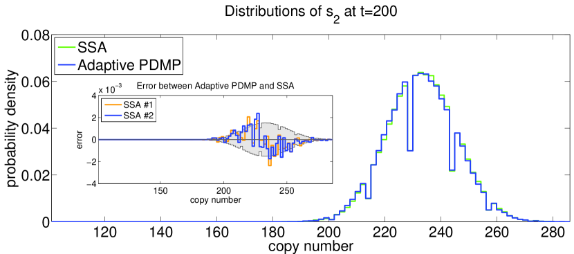
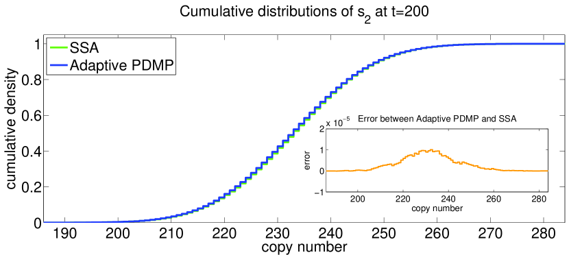
Figure 4: Probability distribution of the Fast Dimerization SRN

The upper plot shows the copy-number distribution (100 equally spaced bins) of species $s_{2}$ at time $t=200$ with SSA (green) and with our Adaptive PDMP scheme (blue). The inset shows the error compared to two independent runs with SSA, each with $100^{\prime}000$ samples. The grey shaded area marks the 95% confidence interval of the SSA run #1.

The lower plot shows the cumulative copy-number distributions of species $s_{2}$ at time $t=200$ with SSA (green) and with our Adaptive PDMP scheme (blue).

V.1.1 Comparison to an existing adaptive PDMP method

We compare our Adaptive PDMP scheme with an existing adaptive PDMP method proposed by Alfonsi et al. alfonsi2005 . We implemented the method similarly to our own implementation and added the necessary details. We compare both methods with SSA for the Fast Dimerization SRN without averaging.

Figure 5 shows the results of $10^{\prime}000$ sample paths for each method. One can clearly see a good match of our method with SSA. The results from the method by Alfonsi et al. are inaccurate. In this case, we suspect that this is due to the partitioning criteria that only considers the copy-number of reactants. Because of this the reaction $s_{1}\rightarrow s_{2}$ is considered as being continuous when the copy-number of $s_{1}$ is big enough. Thus the stochastic variation in species $s_{2}$ is strongly reduced in comparison to the exact SSA simulations.

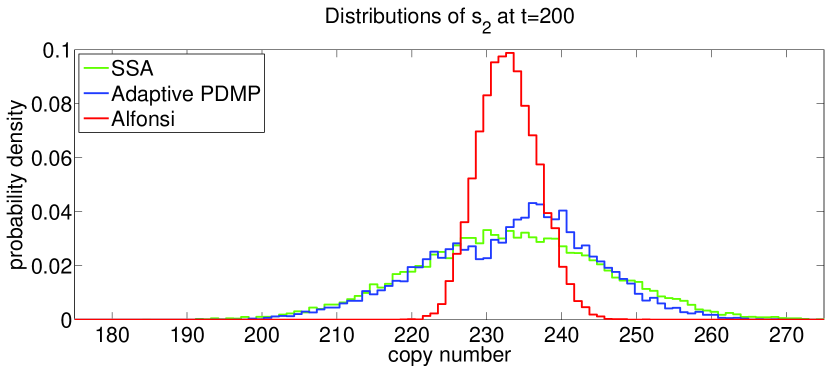
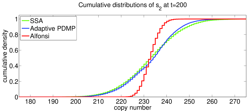
Figure 5: Comparison of the probability distribution of the Fast Dimerization SRN

The upper plot shows the copy-number distribution (100 equally spaced bins) of species $s_{2}$ at time $t=200$ with SSA (green), with our Adaptive PDMP (blue) and with the Alfonsi scheme (red).

The lower plot shows the cumulative copy-number distributions of species $s_{2}$ at time $t=200$ with SSA (green), with our Adaptive PDMP (blue) and with the Alfonsi scheme (red).

V.2 Toggle Switch

We consider the Toggle-Switch network, which is similar to the synthetic Toggle-Switch by Gardner et al.Gardner2000 , but implemented with mass-action kinetics. It consists of $n_{S}=6$ species $m_{A}$, $s_{A}$, $m_{B}$, $s_{B}$, $p_{A}$, $p_{B}$ and $n_{R}=16$ reactions and is depicted in Figure 6. The reactions are listed in Table 4.

Reaction	$\kappa^{\prime}$	Reaction	$\kappa^{\prime}$	Reaction	$\kappa^{\prime}$
$\emptyset\ \rightarrow\ m_{A}$	$1.0$	$m_{A}\rightarrow s_{A}$	$5.0$	$s_{A}\rightarrow\emptyset$	$0.01$
$\emptyset\rightarrow m_{B}$	$1.0$	$m_{B}\rightarrow s_{B}$	$5.0$	$s_{B}\rightarrow\emptyset$	$0.01$
$m_{A}\rightarrow\emptyset$	$0.1$	$s_{A}+m_{B}\rightarrow s_{A}$	$20.0$	$s_{A}\rightarrow s_{A}+p_{A}$	$10.0$
$m_{B}\rightarrow\emptyset$	$0.1$	$s_{B}+m_{A}\rightarrow s_{B}$	$20.0$	$s_{B}\rightarrow s_{B}+p_{B}$	$10.0$
$p_{A}\rightarrow\emptyset$	$0.1$	$p_{B}\rightarrow\emptyset$	$0.1$

Table 4: Reactions of the Toggle Switch network

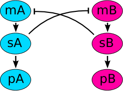
Figure 6: Cartoon of the Toggleswitch network

We estimate the solution given by the CME at time $t_{f}=10^{5}$ where the initial state is set to $x_{0}=\left(0,\ldots,0\right)$. As our scheme could not find any suitable subnetworks for this example, we turned off the averaging procedure to reduce the computational overhead. There are two high copy-number proteins, $p_{A}$ and $p_{B}$, which are controlled by two low copy-number mRNAs, $s_{A}$ and $s_{B}$. These mRNAs $s_{A}$ and $s_{B}$ are the processed variants of the precursor mRNAs $m_{A}$ and $m_{B}$. In addition to inducing translation the mRNAs, $s_{A}$ and $s_{B}$ also induce the degradation of $m_{A}$ and $m_{B}$ respectively. The network shows a bistable behaviour and can stochastically switch between a high copy-number $p_{A}$, low copy-number $p_{B}$ state and a low copy-number $p_{A}$, high copy-number $p_{B}$ state. While the SSA will spend a major part of the simulation time for simulating the translation and degradation of the $p_{A}$ and $p_{B}$ proteins, our adaptive PDMP scheme performs those reactions with continuous dynamics when the proteins have a high copy-number, yielding a considerable performance gain.

The simulation of $100^{\prime}000$ sample paths with SSA took a total CPU time of $\approx 47.4\text{ days}$. The simulation of $100^{\prime}000$ sample paths with our Adaptive PDMP scheme using a step size of $dt=5.0$ took a total CPU time of $\approx 1.1\text{ days}$. Figure 7 shows the results of these simulations. The distribution given by the CME (estimated with SSA) closely matches the distribution estimated with our Adaptive PDMP scheme at time $t=25^{\prime}000$. The Kolmogorov-Smirnov distance between the two distributions is $d_{KS}=0.01$.

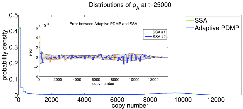
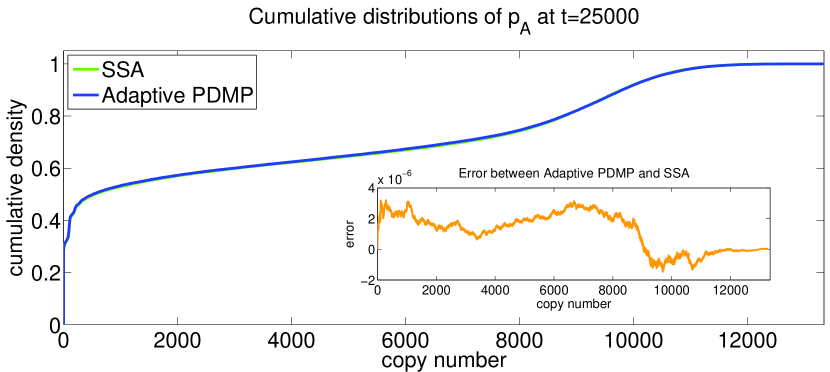
Figure 7: Probability distribution of the Toggleswitch SRN

The upper plot shows the copy-number distribution (100 equally spaced bins) of species $p_{A}$ at time $t=25^{\prime}000$ with SSA (green) and with our Adaptive PDMP scheme (blue). The inset shows the error compared to two independent runs with SSA, each with 100’000 samples. The grey shaded area marks the 95% confidence interval of the SSA run #1. The lower plot shows the cumulative copy-number distributions of species $p_{A}$ at time $t=25^{\prime}000$ with SSA (green) and with our Adaptive PDMP scheme (blue).

V.3 Repressilator

We consider the Repressilator network, which is similar to the synthetic Repressilator by Elowitz et al.elowitz2000synthetic , but implemented with mass-action kinetics. It consists of $n_{S}=6$ species $m_{A}$, $p_{A}$, $m_{B}$, $p_{B}$, $m_{C}$, $p_{C}$ and $n_{R}=15$ reactions and is depicted in Figure 8. The reactions are listed in Table 5.

Reaction	$\kappa^{\prime}$	Reaction	$\kappa^{\prime}$	Reaction	$\kappa^{\prime}$
$\emptyset\rightarrow m_{A}$	$0.1$	$\emptyset\rightarrow m_{B}$	$0.1$	$\emptyset\rightarrow m_{C}$	$0.1$
$m_{A}\rightarrow m_{A}+p_{A}$	$50.0$	$m_{B}\rightarrow m_{B}+p_{B}$	$50.0$	$m_{C}\rightarrow m_{C}+p_{C}$	$50.0$
$m_{A}\rightarrow\emptyset$	$0.01$	$m_{B}\rightarrow\emptyset$	$0.01$	$m_{C}\rightarrow\emptyset$	$0.01$
$m_{A}+p_{B}\rightarrow p_{B}$	$50.0$	$m_{B}+p_{C}\rightarrow p_{C}$	$50.0$	$m_{C}+p_{A}\rightarrow p_{A}$	$50.0$
$p_{A}\rightarrow\emptyset$	$0.01$	$p_{B}\rightarrow\emptyset$	$0.01$	$p_{C}\rightarrow\emptyset$	$0.01$

Table 5: Reactions of the Repressilator network

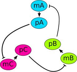
Figure 8: Cartoon of the Repressilator network

We estimate the solution given by the CME at time $t_{f}=5\times 10^{4}$ where the initial state is set to $x_{0}=\left(10,500,0,0,0,0\right)$. Also in this example, there were no suitable subnetworks for the averaging procedure, so we reduced the computational overhead by turning it off.

The Repressilator consists of three mRNAs $m_{A}$, $m_{B}$ and $m_{C}$ and the three corresponding proteins $p_{A}$, $p_{B}$ and $p_{C}$. Each protein catalyses the degradation of another mRNA in a circular manner, that is, $p_{A}$ degrades $m_{C}$, $p_{B}$ degrades $m_{A}$ and $p_{C}$ degrades $m_{B}$. In the stochastic setting, this network exhibits spontaneous oscillatory behaviour (see Figure 9).

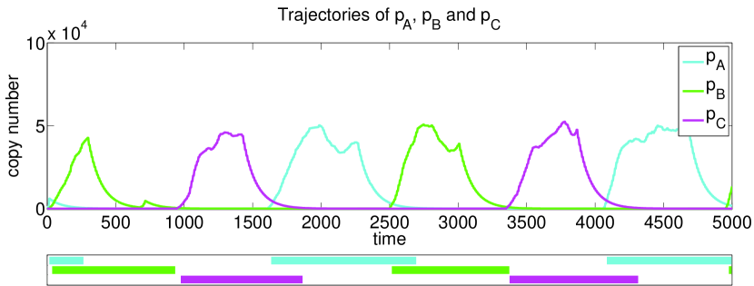
Figure 9: Single trajectory showing the adaptation of our method

Shown is a single sample-path of the copy-number for species $p_{A}$, $p_{B}$ and $p_{C}$ simulated with our Adaptive PDMP scheme. The colored areas below indicate when the corresponding species $p_{X}$ and the reactions $m_{X}\rightarrow m_{X}+p_{X}$ and $p_{X}\rightarrow\emptyset$ are considered to be continuous.

A fixed PDMP scheme that simulates reactions affecting only the protein species continuously (i.e. $p_{X}\rightarrow\emptyset$ and $m_{X}\rightarrow m_{X}+p_{X}$) and the rest discretely, does not exhibit the oscillatory behaviour that can be seen by simulating the SRN with SSA. This can be seen in Figure 10 where the first moment of the copy-number of species $p_{A}$ is shown for different simulation schemes. The result of a fixed PDMP scheme that simulates the translation- and degradation-reaction of species $p_{A}$ with continuous dynamics is shown in red and shows a quick drop of the copy-number to $0$. This is due to the discrete nature of the species in the stochastic description. In the fixed PDMP scheme the protein $p_{A}$ with a very small concentration can still degrade the mRNA $m_{C}$, whereas in the stochastic setting the copy-number of protein $p_{A}$ can drop to $0$ and will not contribute to the degradation of $m_{C}$ anymore, thus enabling $m_{C}$ to rise. On the other hand, when the copy-numbers of the proteins are high, the stochasticity of the translation- and the degradation-reaction is negligible.

Our Adaptive PDMP scheme can approximate the protein dynamics continuously when they have high copy-numbers and switch to discrete stochastic simulations when they have low copy-numbers. This is depicted in Figure 9 where the colored bars indicate when the corresponding degradation- and translation-reactions are approximated with continuous dynamics. One can easily see that the dynamics for the degradation- and translation-reaction of $p_{B}$ is approximated with continuous dynamics when the copy-number of $p_{B}$ is high. In Figure 10 of simulations with SSA (green) and with our adaptive method (blue) show the same oscillatory behaviour. Due to stochasticity the average amplitude decreases with time as the individual trajectories lose their synchronization, unlike the deterministic setting. Note that the initial state is the same for each trajectory. Hence this example illustrates, how an adaptive partitioning scheme can be very useful.

The simulation of $100^{\prime}000$ sample paths with SSA took a total CPU time of $\approx 232\text{ hours}$. The simulation of $100^{\prime}000$ sample paths with our Adaptive PDMP scheme using a step size of $dt=1.0$ took a total CPU time of $\approx 3\text{ hours}$. Figure 11 shows the distribution of species $p_{A}$ at time $t=4^{\prime}750$ for simulations with SSA (green) and with our adaptive scheme (blue). In addition the insets show the deviation from two independent runs with SSA and also mark the 95% confidence intervals (grey area). The distribution given by the CME (estimated with SSA) closely matches the distribution estimated with our Adaptive PDMP scheme at time $t=4^{\prime}750$. The Kolmogorov-Smirnov distance between the two distributions is $d_{KS}=0.003$.

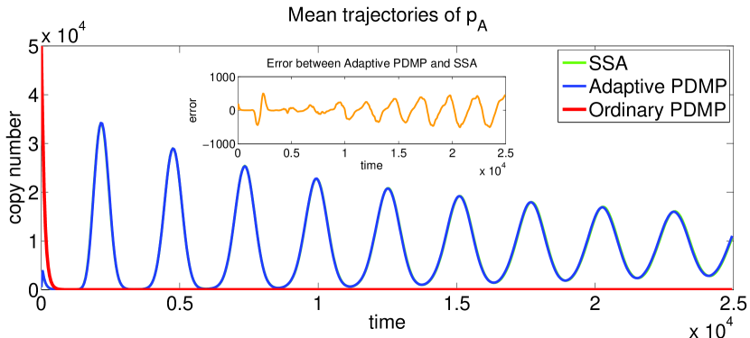
Figure 10: Mean trajectories of species $p_{A}$ for the Repressilator SRN

Shown is the mean of species $p_{A}$ of $100^{\prime}000$ simulations with SSA (green), with the fixed PDMP scheme (red) and with our Adaptive PDMP scheme (blue).

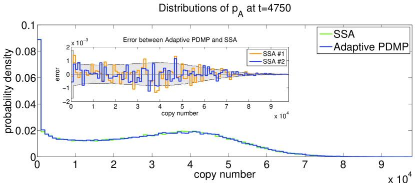
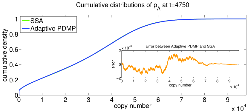
Figure 11: Simulation results of the Repressilator SRN

The upper plot shows the copy-number distribution (100 equally spaced bins) of species $p_{A}$ at time $t=4^{\prime}750$ with SSA (green) and with our Adaptive PDMP scheme (blue). The inset shows the error compared to two independent runs with SSA, each with 100’000 samples. The grey shaded area marks the 95% confidence interval of the SSA run #1.

The lower plot shows the cumulative copy-number distributions of species $p_{A}$ at time $t=4^{\prime}750$ with SSA (green) and with our Adaptive PDMP scheme (blue).

VI Conclusions and future work

In this paper we propose a novel adaptive hybrid scheme for approximating the solution of a Chemical Master Equation for Stochastic Reaction Networks spanning a wide range of reaction timescales, and having large variation in species copy-number scales. The method is based on a rigorous mathematical framework by Kang et al.kang2013separation , that ensures the validity of the approximations.

To achieve considerable speed-ups over SSA our method introduces two sources of error: we treat high copy-number species as continuous and we assume stationarity for the dynamics of fast subnetworks. However with the help of parameters we can tune the amount of error one is willing to tolerate in a qualitative manner. For example, setting $N_{0}\approx\infty$ will reduce our scheme to SSA and setting $\Theta\approx\infty$ would prevent the application of the quasi-stationary assumption.

We compare the results of our adaptive method with SSA and a fixed PDMP scheme using examples from Systems Biology. Our results show that the adaptive method can provide considerable performance enhancements in comparison to both these approaches. Moreover, as our last example demonstrates, the adaptivity can be crucial to achieve accuracy and reduce the computational cost at the same time.

The adaptive feature of our method makes it particularly well suited for SRNs where the timescales of the reaction dynamics can change with time. Such behaviour can be expected in regulatory gene expression networks. We hope that our method will provide a tool for researchers to analyse more complicated and realistic models in Systems Biology.

Our adaptive scheme can potentially be used in the simulation of large scale compartment models of Spatial SRNs elf2004spontaneous . For such systems the spatial distribution of species can change with time and our adaptive method could reduce the computational costs significantly. For example, in the Min System in E. coli fange2006noise , the location of high copy-number species is constantly changing. So an adaptive approach could neglect the fluctuations at these locations, while conserving the fluctuations at locations with low copy-numbers. In the future we aim to develop such adaptive schemes for Spatial SRNs.

Another direction for further research is a combination of our method with a $\tau$-leaping scheme, as we propose in Section IV, and the corresponding study of the mathematical validity of such an approach.

Appendix A Averaging of fast subnetworks

We now describe the averaging procedure for fast subnetworks in this section which is an optional extension to the previously discussed approximation of SRNs.

To check if a subnetwork has fast dynamics in comparison to the surrounding network (which consists of species that are directly influenced by the subnetwork) we look at two sets of reactions, the reactions within the subnetwork, and the reactions connecting the subnetwork to the surrounding network. We then define a timescale for both these sets of reactions and describe a formal criterion to check whether the subnetwork is fast.

As an example, Figure 12 shows a network where a transcription factor switches between an active (tf*) and an inactive (tf) form. In the active form it can bind to a gene and initiate transcription. Assuming that the switch between the active and inactive form of the transcription factor is fast in comparison to the binding of the active transcription factor to the gene, the red reaction would define a fast subnetwork. The orange species make up the fast subnetwork and the blue species make up the surrounding network. The green reaction connects the subnetwork to the surrounding network.

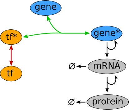
Figure 12: Example network depicting a fast subnetwork and the corresponding reactions

Now we describe this procedure elaborately. Consider a subnetwork with $m_{R}$ reactions $R\subseteq\left\{1,\ldots,n_{R}\right\}$. We define the set of species involved in the reactions in $R$ as

$$Q\left(R\right)=\left\{i:\xi_{ik}\neq 0\text{ for some }k\in R\right\}$$

and define the set of species that are catalytically involved in the reactions in $R$ as

$$Q_{C}\left(R\right)=\left\{i\not\in Q\left(R\right):\nu_{ik}=\nu^{\prime}_{ik}>0\text{ for some }k\in R\right\}.$$

Note that the propensities of the reactions in $R$ only depend on the species in $Q\left(R\right)$ and $Q_{C}\left(R\right)$. Assume that the copy-numbers of the species in $Q_{C}\left(R\right)$ are constant. Then the reactions in $R$ and the species in $Q\left(R\right)$ naturally define a SRN. Suppose that the dynamics of this SRN converges to a unique stationary distribution for any choice of copy-numbers of the species in $Q_{C}\left(R\right)$. If the reactions in $R$ are sufficiently faster than the surrounding reactions, given by

$$R_{S}\left(R\right)= \left\{k\not\in R:\nu_{ik}>0\text{ or }\nu^{\prime}_{ik}>0\text{ for some }i\in Q\left(R\right)\right\}$$

$$\cup \left\{k\not\in R:\xi_{ik}\neq 0\text{ for some }i\in Q_{C}\left(R\right)\right\},$$

then the stationary distribution of the subnetwork can be used to compute the propensities of the reactions in $R_{S}\left(R\right)$. This is called the quasi-stationary assumption Cao2005 .

We now specify a formal criteria to check if the subnetwork dynamics is sufficiently fast in comparison to its surrounding network. For this we define a timescale for each reaction $k$ as

$$\zeta\left(k\right)=\frac{\log\kappa^{\prime}_{k}}{\log N_{0}}+\sum_{i=1}^{n_{S}}\nu_{ik}\cdot\frac{\log x_{i}}{\log N_{0}}\cdot\mathds{1}_{\left\{x_{i}>0\right\}}\\$$

and the observation timescale as $\zeta\left(0\right)=\frac{\log\left(1/t_{f}\right)}{\log{N_{0}}}$. The form of $\zeta\left(k\right)$ is chosen in such a way that $N_{0}^{\zeta\left(k\right)}$ captures the timescale of the $k$-th reaction channel. However, when reaction channel $k$ consumes a species $i$ (i.e. $\xi_{ik}<0$) and the copy-number $x_{i}=0$, then the exponent to $N_{0}$ would have to be $-\infty$ to exactly capture the timescale of the $k$-th reaction channel. A single reaction producing species $i$ would then change the timescale to a finite value and immediately render the averaging decision based on the timescale as invalid. To prevent this we overestimate the timescale of a reaction channel by ignoring the $-\infty$ terms when computing $\zeta\left(k\right)$. This is achieved by adding the indicator functions $\mathds{1}_{\left\{x_{i}>0\right\}}$ in $\zeta\left(k\right)$.

The timescale separation of the fast subnetwork is then given by

$$\Delta\zeta\left(R\right)=\min_{k\in R}\left(\zeta\left(k\right)\right)-\max_{k\in R_{S}\left(R\right)\cup\left\{0\right\}}\left(\zeta\left(k\right)\right)\quad.$$ (15)

In words, $\Delta\zeta\left(R\right)$ is the difference between the slowest timescale of all reactions within the subnetwork and the fastest timescale of all reactions connecting the subnetwork to the surrounding network. We fix a positive parameter $\Theta$ (with $\Theta=0.5$ as the default value). If $\Delta\zeta\left(R\right)\geq\Theta$ then we call the subnetwork defined by $R$ and $Q\left(R\right)$ to be fast.

Given that a subnetwork is fast, we can apply the quasi-stationary assumption if the dynamics of this subnetwork converges to a stationary distribution. Below we describe three different strategies to check if this is indeed the case.

Finite Markov Chains

Suppose that the species in $Q\left(R\right)$ satisfy a conservation relation of the form $\sum_{i\in Q\left(R\right)}b_{i}x_{i}=C$, where the $b_{i}$-s and $C$ are positive integers and assume that the copy-numbers of species outside $Q\left(R\right)$ are fixed. Due to the reactions in $R$ the copy-number vector of all the species is constrained to reside in a finite set, which can be enumerated as $\left\{e_{1},\ldots,e_{L}\right\}$. Define a $L\times L$ matrix $A$ with entries given by

$$A_{ij}=\begin{cases}\sum_{R_{ij}}\lambda^{\prime}_{k}\left(e_{i}\right)&\text{ if }i\neq j\\ -\sum_{k\in R}\lambda^{\prime}_{k}\left(e_{i}\right)&\text{ if }i=j\\ \end{cases}$$

where $R_{ij}=\left\{k\in R:e_{i}+\xi_{k}=e_{j}\right\}$. If there exists a unique positive vector $\pi=\left(\pi_{1},\ldots,\pi_{L}\right)$ such that $\sum_{i=1}^{L}\pi_{i}=1$ and $\pi A=0$, then the Markov process corresponding to the subnetwork dynamics is ergodic with the unique stationary distribution given by the vector $\pi$. One can check the existence and uniqueness of $\pi$ by verifying that the dimension of the left null-space of $A$ is one seneta2006 .

Pseudo-Linear subnetworks

Consider the subnetwork defined by $R$ and $Q\left(R\right)$ as before. Assume that the propensities of the reactions in $R$ are affine functions of the copy-numbers of the species in $Q\left(R\right)$, that is $\sum_{i\in Q\left(R\right)}\nu_{ik}\leq 1$ for all $k\in R$. Such a subnetwork is called pseudo-linear because it does not involve any bimolecular reactions between the fast species in the subnetwork. For linear networks the moment equations are closed. Hence we can easily find the first two stationary moments by finding the fixed points of the moment equations

$$\frac{d\mathbb{E}[X_{i}]}{dt}= \sum_{k\in R}\xi_{ik}\mathbb{E}[\lambda^{\prime}_{k}\left(X\right)]$$

$$\frac{d\mathbb{E}[X_{i}X_{j}]}{dt}= \sum_{k\in R}\xi_{ik}\mathbb{E}[\lambda^{\prime}_{k}\left(X\right)X_{j}]+\sum_{k\in R}\mathbb{E}[\lambda^{\prime}_{k}\left(X\right)X_{i}]\xi_{jk}+\sum_{k\in R}\xi_{ik}\mathbb{E}[\lambda^{\prime}_{k}\left(X\right)]\xi_{jk},$$

and checking if these fixed points are stable. As we only consider at most bimolecular reactions we only need the first two stationary moments to apply the quasi-stationary assumption.

Zero-Deficiency subnetworks

In some situations, a fast subnetwork may not be pseudo-linear and its state space is either infinite or too large to be able to compute the exact stationary distribution for the corresponding Markov Chain (for example see the Fast Dimerization network in Section V). In such cases it is sometimes possible to use the recent results from Anderson et al.anderson_kurtz_2010  to compute the stationary distribution of the subnetwork dynamics. In particular Anderson et al.anderson_kurtz_2010  show that weakly reversible networks with zero deficiency admit a product-form stationary distribution given by

$$\pi\left(x\right)=M\prod_{i\in Q\left(R\right)}\frac{c_{i}^{x_{i}}}{x_{i}!},\quad x\in\Gamma$$ (16)

and $\pi\left(x\right)=0$ otherwise, where $\Gamma$ is an irreducible state space containing the initial state, $c\in\mathbb{R}_{\geq 0}^{n_{S}}$ is the equilibrium point of the corresponding deterministic system and $M$ is a positive normalizing constant. We can find the appropriate set $\Gamma$ using the results in gupta2013determining , and this would imply that the dynamics of the distribution of the SRN will converge to the stationary distribution $\pi$.

Implementation details

During the simulation of the sample path we need to keep track of changes to the copy-numbers of species in $Q\left(R\right)$, so that we can recompute the moments of the stationary distribution of the fast subnetwork. We do this by modifying the partitioning of the reactions, so that the reactions in $R_{S}\left(R\right)$ are discrete. Every time a reaction in $k\in R_{S}\left(R\right)$ occurs, the first and second moments of the stationary distribution are recomputed and the appropriate rate constants are updated. For this, Algorithm 2 has to be modified in a straightforward manner. Below we describe the averaging procedure.

Algorithm 4: Averaging

1. Once: Precompute subnetworks $L_{A}$ suitable for averaging
   (e.g. weakly reversible, zero-deficiency subnetworks)

2. Let $L_{P}$ be the set of previously averaged subnetworks

3. Set $L_{C}=\emptyset$

4. for each suitable subnetwork $R\in L_{A}$ do

5. if $\Delta\zeta\left(R\right)\geq\Theta$ then

6. Set $L_{C}=L_{C}\cup\left\{R\right\}$

7. end if

8. end for

9. $L_{F}=\emptyset$

10. while $L_{C}\neq\emptyset$ do

11. Set $R=\operatorname*{argmax}_{W\in L_{C}}\left(|W|\right)$

12. Set $L_{C}=L_{C}\setminus{R}$

13. if $\underset{W\in L_{F}}{\cup}W\cap R=\emptyset$ and
    $\underset{W\in L_{F}}{\cup}Q\left(W\right)\cap Q\left(R\right)=\emptyset$ then

14. Set $L_{F}=L_{F}\cup\left\{R\right\}$

15. Modify $R_{D},R_{C}$, so that $R_{S}\left(R\right)\subseteq R_{D}$

16. end if

17. end while

18. for each subnetwork $R\in L_{P}\setminus L_{F}$ do

19. Sample state of the species in $Q\left(R\right)$ from the
    stationary distribution

20. end for

21. for each subnetwork $R\in L_{F}$ do

22. Compute stationary first and second moment of the
    species in $Q\left(R\right)$

23. Update the stoichiometries and propensities of
    reactions in $R_{S}\left(R\right)$

24. end for

Appendix B Mathematical Justification

In this section we provide a mathematical justification of why our adaptive scheme produces a close approximation to the solution of a CME. We start with a simple lemma that shows convergence of a sequence of processes, in which each process is formed by stitching together two Markov processes at a random stopping time determined by the first process. In this section let $n=n_{S}$, where $n_{S}$ is the number of species, and let “$\Rightarrow$” and “$\approx_{d}$” denote convergence in distribution and similarity in distribution respectively. Let $\mathbb{D}_{\mathbb{R}^{n}}[0,\infty)$ denote the space of càdlàg functions, from $[0,\infty)$ to $\mathbb{R}^{n}$, that is, right continuous functions with left limits ethier2009markov . Let $A$ be a measurable subset of $\mathbb{R}^{n}$ and define $\mathcal{G}_{A}:\mathbb{D}_{\mathbb{R}^{n}}\left[0,\infty\right)\rightarrow[0,\infty]$ by

$$\mathcal{G}_{A}\left(\zeta\right)=\inf\left\{t\geq 0:\zeta\left(t\right)\not\in A\right\}.$$ (17)

For each $N$, let $W_{1}^{N},W_{2}^{N}$ be two Markov processes with sample paths in $\mathbb{D}_{\mathbb{R}^{n}}\left[0,\infty\right)$. Assume that for any sequence of initial conditions satisfying $W_{i}^{N}\left(0\right)\Rightarrow W_{i}\left(0\right)$ we have $W_{i}^{N}\Rightarrow W_{i}$ as $N\rightarrow\infty$, where $W_{i}$ is a PDMP as in (5). Define a stopping time $\tau^{N}=\mathcal{G}_{A}\left(W_{1}^{N}\right)$. Suppose $W_{1}^{N}\left(0\right)=w_{0}$ and $W_{2}^{N}\left(0\right)=f\left(W_{1}^{N}\left(\tau^{N}\right)\right)$, where $f:\mathbb{R}^{n}\rightarrow\mathbb{R}^{n}$ is a measurable function.

Define another process $W^{N}$ by

$$W^{N}\left(t\right)=W_{1}^{N}\left(t\right)\mathds{1}_{\left\{t<\tau^{N}\right\}}+W_{2}^{N}\left(t-\tau^{N}\right)\mathds{1}_{\left\{t\geq\tau^{N}\right\}}$$

Lemma.

For any $t\geq 0$ we have

$$W^{N}\left(t\right)\Rightarrow W\left(t\right)$$

where

$$W\left(t\right)=W_{1}\left(t\right)\mathds{1}_{\left\{t<\tau\right\}}+W_{2}\left(t-\tau\right)\mathds{1}_{\left\{t\geq\tau\right\}}$$

with $\tau=\mathcal{G}_{A}\left(W_{1}\right)$, $W_{1}\left(0\right)=w_{0}$ and $W_{2}\left(0\right)=f\left(W_{1}\left(\tau\right)\right)$.

Proof.

Let $g:\operatorname*{\mathbb{R}}^{n}\to\operatorname*{\mathbb{R}}^{n}$ be any bounded continuous function. To prove the lemma it suffices to show that for any $t\geq 0$

$$\lim_{N\to\infty}\operatorname*{\mathbb{E}}(g(W^{N}(t)))=\operatorname*{\mathbb{E}}(g(W(t))),$$ (18)

where $\operatorname*{\mathbb{E}}$ denotes the expectation operator. Fix a $t\geq 0$. We can write

$$\operatorname*{\mathbb{E}}\left(g(W^{N}(t))\right) =\operatorname*{\mathbb{E}}\left(g(W^{N}(t))\mathds{1}_{\{t<\tau^{N}\}}+g(W^{N}(t))\mathds{1}_{\{t\geq\tau^{N}\}}\right)$$ (19)

$$=\operatorname*{\mathbb{E}}\left(g(W^{N}_{1}(t))\mathds{1}_{\{t<\tau^{N}\}}+g(W^{N}_{2}(t-\tau^{N}))\mathds{1}_{\{t\geq\tau^{N}\}}\right).$$

Note that $\tau^{N}=\mathcal{G}_{A}(W^{N}_{1})$ and $W^{N}_{1}\Rightarrow W_{1}$, where $W_{1}$ is a PDMP. Hence, we can conclude that $(W^{N}_{1},\tau^{N})\Rightarrow(W_{1},\tau)$, where $\tau=\mathcal{G}_{A}(W_{1})$. This shows that

$$\lim_{N\to\infty}\operatorname*{\mathbb{E}}\left(g(W^{N}_{1}(t))\mathds{1}_{\{t<\tau^{N}\}}\right)=\operatorname*{\mathbb{E}}\left(g(W_{1}(t))\mathds{1}_{\{t<\tau\}}\right).$$ (20)

The second term in (19) can be expressed as

$$\operatorname*{\mathbb{E}}\left(g(W^{N}_{2}(t-\tau^{N}))\mathds{1}_{\{t\geq\tau^{N}\}}\right)=\operatorname*{\mathbb{E}}\left(\operatorname*{\mathbb{E}}\left(g(W^{N}_{2}(t-\tau^{N}))\mathds{1}_{\{t\geq\tau^{N}\}}|W^{N}_{1}(\tau^{N})\right)\right)$$

Given $W^{N}_{1}(\tau^{N})=w$, the process $W^{N}_{2}$ converges in distribution to the PDMP $W_{2}$ with initial state $f(w)$. Moreover, the results in baxter1977compactness show that $W^{N}_{1}(\tau^{N})\Rightarrow W_{1}(\tau)$. Therefore

$$\lim_{N\to\infty}\operatorname*{\mathbb{E}}\left(g(W^{N}_{2}(t-\tau^{N}))\mathds{1}_{\{t\geq\tau^{N}\}}\right) =\operatorname*{\mathbb{E}}\left(\operatorname*{\mathbb{E}}\left(g(W_{2}(t-\tau))\mathds{1}_{\{t\geq\tau\}}|W_{1}(\tau)\right)\right)$$

$$=\operatorname*{\mathbb{E}}\left(g(W_{2}(t-\tau))\mathds{1}_{\{t\geq\tau\}}\right).$$

Using this relation along with (20) and (19) we obtain

$$\lim_{N\to\infty}\operatorname*{\mathbb{E}}\left(g(W^{N}(t))\right)=\operatorname*{\mathbb{E}}\left(g(W_{1}(t))\mathds{1}_{\{t<\tau\}}\right)+\operatorname*{\mathbb{E}}\left(g(W_{2}(t-\tau))\mathds{1}_{\{t\geq\tau\}}\right)=\operatorname*{\mathbb{E}}(g(W(t))).$$

This shows (18) and finishes the proof of this lemma. ∎

The above lemma can be easily generalized to the more general case, where $W^{N}$ is defined by stitching together $m$ Markov processes $W_{1}^{N},\ldots,W_{m}^{N}$, where each $W_{i}^{N}$ converges to a PDMP $W_{i}$. We define $\tau_{0}^{N}=0$ and $\tau_{i}^{N}=\tau_{i-1}^{N}+\mathcal{G}_{A}\left(W_{i}^{N}\right)$, and similarly $\tau_{0}=0$ and $\tau_{i}=\tau_{i-1}+\mathcal{G}_{A}\left(W_{i}\right)$ for $i=1,\ldots,(m-1)$. The initial states of the processes $W_{i}^{N}$ and $W_{i}$ are given by $W_{i}^{N}\left(0\right)=f_{i}\left(W_{i-1}^{N}\left(\tau_{i-1}^{N}\right)\right)$ and $W_{i}\left(0\right)=f_{i}\left(W_{i-1}\left(\tau_{i-1}\right)\right)$ respectively, for $i=2,\ldots,m$, where $f_{i}:\mathbb{R}^{n}\rightarrow\mathbb{R}^{n}$ are measurable functions. Assuming $W^{N}_{1}\left(0\right)\Rightarrow W_{1}\left(0\right)$, the process $W^{N}$ given by

$$W^{N}\left(t\right)=\sum_{i=1}^{m}W_{i}^{N}\left(t-\tau_{i-1}^{N}\right)\mathds{1}_{\left\{\tau_{i-1}^{N}\leq t<\tau_{i}^{N}\right\}}$$ (21)

converges in distribution to the process $W$ defined by

$$W\left(t\right)=\sum_{i=1}^{m}W_{i}\left(t-\tau_{i-1}\right)\mathds{1}_{\left\{\tau_{i-1}\leq t<\tau_{i}\right\}}.$$ (22)

In our adaptive scheme the times of adaptation are defined analogously to (17) where the set $A$ is given by (12). We denote the times of adaptation by $\tau_{i}^{N}$ for $i=1,\ldots,(m-1)$, where $(m-1)$ is the number of adaptations. We define $\tau_{0}^{N}=0$ and $\tau_{m}^{N}=\infty$ for convenience. The computation of the scaling parameters $\alpha=\left(\alpha_{1},\ldots,\alpha_{n}\right)$ and $\beta=\left(\beta_{1},\ldots,\beta_{n_{R}}\right)$ only depends on the state of the simulated process at the time of adaptation. Suppose that this computation is given by functions $L_{\alpha},L_{\beta}:\mathbb{R}^{n}\rightarrow\mathbb{R}^{n}$, such that for $\tau_{i}^{N}\leq t<\tau_{i+1}$ we have $\alpha\left(t\right)=L_{\alpha}\left(W^{N}\left(\tau_{i}^{N}\right)\right)$ and $\beta\left(t\right)=L_{\beta}\left(W_{i}^{N}\left(\tau_{i}^{N}\right)\right)$. Here $W^{N}$ denotes the adaptive version of the scaled family of processes in (3). We can write $W^{N}$ in the form (21) with

$$W_{i}^{N}\left(t\right) =W^{N}_{i}\left(0\right)+N^{-\alpha\left(\tau^{N}_{i-1}\right)}\sum_{k=1}^{n_{R}}Y_{k}\left(\int_{0}^{t}N^{\beta\left(\tau^{N}_{i-1}\right)+\alpha\left(\tau^{N}_{i-1}\right)\cdot\nu_{k}}\lambda_{k}^{N}\left(W_{i}^{N}(s\right)ds\right)\xi_{k}$$

where $N^{x}=\operatorname*{diag}\left(N^{x_{1}},\ldots,N^{x_{k}}\right)$ for a $k$-dimensional vector $x=\left(x_{1},\ldots,x_{k}\right)$. The initial conditions are given by $W^{N}_{1}\left(0\right)=N_{0}^{-\alpha\left(0\right)}X\left(0\right)$ and $W^{N}_{i}\left(0\right)=N_{0}^{\alpha\left(\tau^{N}_{i-1}\right)-\alpha\left(\tau^{N}_{i}\right)}W_{i}^{N}\left(\tau^{N}_{i}\right)$ for $i=2,\ldots,m$. From Kang et al.kang2013separation  we know that each $W^{N}_{i}$ converges in distribution to a PDMP $W_{i}$, as described in Section II. From the previous lemma it follows that $W^{N}\left(t\right)\Rightarrow W\left(t\right)$ for any $t\geq 0$, where $W$ has the form (22) with the $W_{i}$-s given by the convergence result of Kang et al.kang2013separation , given in II.

Now we return to our original process $X$ from Section II and recall that for large $N_{0}$ we have $X\left(t\right)=N_{0}^{\alpha}Z^{N_{0}}\left(t\right)\approx_{d}N_{0}^{\alpha}Z\left(t\right)$. With adaptation we also have $X\left(t\right)=N_{0}^{\alpha}W^{N_{0}}\left(t\right)$ and as $W^{N}\left(t\right)\Rightarrow W\left(t\right)$ for any $t\geq 0$, it follows that $X\left(t\right)=N_{0}^{\alpha}W^{N_{0}}\left(t\right)\approx_{d}N_{0}^{\alpha}W\left(t\right)$ and this justifies the use of our adaptive scheme to approximate the distribution of the original process $X$ at any fixed time $t\geq 0$.

References

- (1) J. Goutsias, “Classical versus stochastic kinetics modeling of biochemical reaction systems,” Biophysical journal, vol. 92, no. 7, pp. 2350–2365, 2007.
- (2) H. H. McAdams and A. Arkin, “Stochastic mechanisms in gene expression,” Proceedings of the National Academy of Sciences, vol. 94, no. 3, pp. 814–819, 1997.
- (3) B. Munsky, A. Hernday, D. Low, and M. Khammash, “Stochastic modeling of the pap-pili epigenetic switch,” Proc. FOSBE, pp. 145–148, 2005.
- (4) D. Fange and J. Elf, “Noise-induced Min phenotypes in E. coli,” PLoS computational biology, vol. 2, no. 6, pp. –80, 2006.
- (5) T. S. Gardner, C. R. Cantor, and J. J. Collins, “Construction of a genetic toggle switch in Escherichia coli.,” Nature, vol. 403, pp. 339–42, Jan. 2000.
- (6) M. B. Elowitz and S. Leibler, “A synthetic oscillatory network of transcriptional regulators,” Nature, vol. 403, no. 6767, pp. 335–338, 2000.
- (7) J. Goutsias and G. Jenkinson, “Markovian dynamics on complex reaction networks,” Physics Reports, 2013.
- (8) B. Munsky and M. Khammash, “The finite state projection algorithm for the solution of the chemical master equation,” The Journal of chemical physics, vol. 124, p. 044104, 2006.
- (9) V. Kazeev, M. Khammash, M. Nip, and C. Schwab, “Direct solution of the Chemical Master Equation using quantized tensor trains.,” PLoS computational biology, vol. 10, p. e1003359, Mar. 2014.
- (10) D. T. Gillespie, “Stochastic simulation of chemical kinetics,” Annu. Rev. Phys. Chem., vol. 58, pp. 35–55, 2007.
- (11) W. E, D. Liu, and E. Vanden-Eijnden, “Nested stochastic simulation algorithm for chemical kinetic systems with disparate rates.,” The Journal of chemical physics, vol. 123, p. 194107, Nov. 2005.
- (12) Y. Cao, D. T. Gillespie, and L. R. Petzold, “The slow-scale stochastic simulation algorithm.,” The Journal of chemical physics, vol. 122, p. 14116, Jan. 2005.
- (13) D. T. Gillespie, “Approximate accelerated stochastic simulation of chemically reacting systems,” The Journal of Chemical Physics, vol. 115, p. 1716, 2001.
- (14) Y. Cao, D. T. Gillespie, and L. R. Petzold, “Efficient step size selection for the tau-leaping simulation method,” The Journal of chemical physics, vol. 124, p. 044109, 2006.
- (15) Y. Cao, D. T. Gillespie, and L. R. Petzold, “Adaptive explicit-implicit tau-leaping method with automatic tau selection,” The Journal of chemical physics, vol. 126, no. 22, p. 224101, 2007.
- (16) M. Rathinam, L. R. Petzold, Y. Cao, and D. T. Gillespie, “Stiffness in stochastic chemically reacting systems: The implicit tau-leaping method,” The Journal of Chemical Physics, vol. 119, p. 12784, 2003.
- (17) T. G. Kurtz, “Strong approximation theorems for density dependent Markov chains,” Stochastic Processes and Their Applications, vol. 6, no. 3, pp. 223–240, 1978.
- (18) The concentration is the copy-number divided by the volume of the system.
- (19) H.-W. Kang and T. G. Kurtz, “Separation of time-scales and model reduction for stochastic reaction networks,” The Annals of Applied Probability, vol. 23, no. 2, pp. 529–583, 2013.
- (20) A. Crudu, A. Debussche, and O. Radulescu, “Hybrid stochastic simplifications for multiscale gene networks,” BMC systems biology, vol. 3, no. 1, p. 89, 2009.
- (21) M. H. Davis, “Piecewise-deterministic Markov processes: A general class of non-diffusion stochastic models,” Journal of the Royal Statistical Society. Series B (Methodological), pp. 353–388, 1984.
- (22) E. L. Haseltine and J. B. Rawlings, “Approximate simulation of coupled fast and slow reactions for stochastic chemical kinetics,” The Journal of chemical physics, vol. 117, no. 15, pp. 6959–6969, 2002.
- (23) J. Pahle, Eine Hybridmethode zur Simulation biochemischer Prozesse. PhD thesis, Diploma thesis, ILKD, Universität Karlsruhe (TH) and EML, Heidelberg, 2002.
- (24) N. A. Neogi, “Dynamic partitioning of large discrete event biological systems for hybrid simulation and analysis,” in Hybrid Systems: Computation and Control, pp. 463–476, Springer, 2004.
- (25) M. Bentele and R. Eils, “General stochastic hybrid method for the simulation of chemical reaction processes in cells,” in Computational Methods in Systems Biology, pp. 248–251, Springer, 2005.
- (26) H. Salis and Y. Kaznessis, “Accurate hybrid stochastic simulation of a system of coupled chemical or biochemical reactions,” The Journal of chemical physics, vol. 122, p. 054103, 2005.
- (27) A. Crudu, A. Debussche, A. Muller, and O. Radulescu, “Convergence of stochastic gene networks to hybrid piecewise deterministic processes,” The Annals of Applied Probability, vol. 22, no. 5, pp. 1822–1859, 2012.
- (28) A. Alfonsi, E. Cancès, G. Turinici, B. Di Ventura, and W. Huisinga, “Adaptive simulation of hybrid stochastic and deterministic models for biochemical systems,” in ESAIM: Proceedings, vol. 14, pp. 1–13, EDP Sciences, 2005.
- (29) S. Hoops, R. Gauges, C. Lee, J. Pahle, N. Simus, M. Singhal, L. Xu, P. Mendes, and U. Kummer, “COPASI - A COmplex PAthway SImulator,” Bioinformatics, vol. 22, pp. 3067–3074, 2006.
- (30) M. Griffith, T. Courtney, J. Peccoud, and W. H. Sanders, “Dynamic partitioning for hybrid simulation of the bistable HIV-1 transactivation network.,” Bioinformatics (Oxford, England), vol. 22, pp. 2782–9, Nov. 2006.
- (31) J. Puchałka and A. M. Kierzek, “Bridging the gap between stochastic and deterministic regimes in the kinetic simulations of the biochemical reaction networks.,” Biophysical journal, vol. 86, pp. 1357–72, Mar. 2004.
- (32) K. Burrage, T. Tian, and P. Burrage, “A multi-scaled approach for simulating chemical reaction systems.,” Progress in biophysics and molecular biology, vol. 85, no. 2-3, pp. 217–34, 2004.
- (33) L. a. Harris and P. Clancy, “A ”partitioned leaping” approach for multiscale modeling of chemical reaction dynamics.,” The Journal of chemical physics, vol. 125, p. 144107, Oct. 2006.
- (34) J. R. Chubb, T. Trcek, S. M. Shenoy, and R. H. Singer, “Transcriptional pulsing of a developmental gene,” Current biology, vol. 16, no. 10, pp. 1018–1025, 2006.
- (35) J. Pahle, “Biochemical simulations: stochastic, approximate stochastic and hybrid approaches.,” Briefings in bioinformatics, vol. 10, pp. 53–64, Jan. 2009.
- (36) C. V. Rao and A. P. Arkin, “Stochastic chemical kinetics and the quasi-steady-state assumption: Application to the Gillespie algorithm,” The Journal of Chemical Physics, vol. 118, no. 11, p. 4999, 2003.
- (37) IUPAC. Compendium of Chemical Terminology, 2nd ed. (the Gold Book). Compiled by A. D. McNaught and A. Wilkinson. Blackwell Scientific Publications, Oxford (1997). XML on-line corrected version: http://goldbook.iupac.org (2006-) created by M. Nic, J. Jirat, B. Kosata; updates compiled by A. Jenkins. ISBN 0-9678550-9-8. doi:10.1351/goldbook.
- (38) D. T. Gillespie, “A diffusional bimolecular propensity function,” The Journal of chemical physics, vol. 131, no. 16, pp. 164109–164109, 2009.
- (39) S. N. Ethier and T. G. Kurtz, Markov processes: characterization and convergence, vol. 282. Wiley. com, 2009.
- (40) S. Peleš, B. Munsky, and M. Khammash, “Reduction and solution of the chemical master equation using time scale separation and finite state projection,” The Journal of chemical physics, vol. 125, no. 20, p. 204104, 2006.
- (41) O. Radulescu, A. N. Gorban, A. Zinovyev, and A. Lilienbaum, “Robust simplifications of multiscale biochemical networks,” BMC systems biology, vol. 2, no. 1, p. 86, 2008.
- (42) The implementation allows different ODE solvers to be used. However, for the examples we used the Dormand-Prince 5 stepper from the boost odeint library (http://www.boost.org/). The boost odeint library is coupled to our implementation via a Java Native Interface wrapper.
- (43) For subnetworks that are weakly reversible and have deficiency zero, we compute the moments of the product-form stationary distribution, where all the species satisfy a conservation relation, by approximating it with a multinomial distribution with appropriately defined virtual species. The error incurred by this approximation is generally small enough to be neglected. If no species satisfy a conservation relation, then the stationary distribution is just the product of independent Poisson distributions.
- (44) J. Elf and M. Ehrenberg, “Spontaneous separation of bi-stable biochemical systems into spatial domains of opposite phases,” Systems biology, vol. 1, no. 2, pp. 230–236, 2004.
- (45) E. Seneta, Non-negative Matrices and Markov Chains (Springer Series in Statistics). Springer, 2006.
- (46) D. F. Anderson, G. Craciun, and T. G. Kurtz, “Product-form stationary distributions for deficiency zero chemical reaction networks,” Bulletin of mathematical biology, vol. 72, no. 8, pp. 1947–1970, 2010.
- (47) A SRN is called weakly reversible if for every reaction there is a sequence of reactions such that and .
- (48) The deficiency of a SRN is defined as where is the number of reaction complexes (), is the number of linkage classes (a linkage class is a connected component of the reaction complex graph corresponding to the SRN) and is the dimension of the stoichiometric subspace . We refer the readers to anderson_kurtz_2010 for more details.
- (49) A. Gupta and M. Khammash, “Determining the long-term behavior of cell populations: A new procedure for detecting ergodicity in large stochastic reaction networks,” arXiv preprint arXiv:1312.2879, 2013.
- (50) J. R. Baxter and R. V. Chacon, “Compactness of stopping times,” Probability Theory and Related Fields, vol. 40, no. 3, pp. 169–181, 1977.