The FastHCS Algorithm for Robust PCA

Abstract

Principal component analysis (PCA) is widely used to analyze high-dimensional data, but it is very sensitive to outliers. Robust PCA methods seek fits that are unaffected by the outliers and can therefore be trusted to reveal them. FastHCS (High-dimensional Congruent Subsets) is a robust PCA algorithm suitable for high-dimensional applications, including cases where the number of variables exceeds the number of observations. After detailing the FastHCS algorithm, we carry out an extensive simulation study and three real data applications, the results of which show that FastHCS is systematically more robust to outliers than state-of-the-art methods.

Keywords: High-dimensional data, outlier detection, computational statistics, exploratory data analysis

1 Introduction

Principal component analysis (PCA) is widely used to explore high-dimensional data. It centers and rotates the original $p$-dimensional measurements to construct a small number $q$ of new orthonormal variables, called principal components, that account for most of the variation in the data. However, classical PCA is very sensitive to outliers. Outliers are observations that are inconsistent with the multivariate pattern of the majority of the data. If left unchecked, they influence the estimated parameters by disproportionately pulling the fit towards themselves. In this way, outliers obscure the main relationships in the data and their true outlyingness. In practice, we want to find the outliers to bound their influence on the fit and to study as objects of interest in their own right. For these reasons, we need robust PCA methods that meet the following criteria: (1) Like classical PCA, a robust PCA method should handle cases where the number of variables exceeds the number of observations, (2) and it should be shift and rotation equivariant, meaning that if the data are shifted or rotated the estimated parameters should transform accordingly. (3) It should be computable for high-dimensional data. (4) It should accurately describe the multivariate pattern of the majority of the observations, even when the data is heavily contaminated by outliers. (5) It should have a high breakdown point; a measure an estimator’s robustness to outliers in the data. (6) It should be insensitive to the dimensionality of the data. Criteria (1)-(3) are natural for any PCA method. Criteria (4)-(5) relate to robustness. Criterion (6) is related to both concerns. We find that state-of-the-art robust PCA algorithms have most of these properties, but that, surprisingly, many instances can be found where they fail to satisfy Criterion (4). In this paper, we introduce a robust PCA algorithm, FastHCS, to meet these criteria (HCS for high-dimensional congruent subset). In the next section we outline FastHCS. Then, in Sections (3) and (4) we compare it to several state-of-the-art methods on simulated data and three real data applications which show that in many settings only FastHCS can be relied upon to provide a robust PCA solution.

2 FastHCS

Given an $n\times p$ data matrix $\boldsymbol{Y}=\{\boldsymbol{y}_{i}\}_{i=1}^{n}$ and for a fixed $2\leqslant q<\min(p,n)$, the FastHCS algorithm searches for a subset of size at least $h=\lceil(n+q+1)/2\rceil$ free of outliers (this is the minimal value of $h$ such that there are at least $(q+1)$ clean observations in each candidate subset).

If $p>n$, FastHCS computes the mean-centered data matrix $\tilde{\boldsymbol{X}}=\boldsymbol{Y}-\boldsymbol{1}_{n}^{\top}(\operatorname*{ave}_{i=1}^{n}\boldsymbol{y}_{i})$, and performs the kernel eigenvalue decomposition of $\tilde{\boldsymbol{X}}\tilde{\boldsymbol{X}}^{\top}=\boldsymbol{U}\boldsymbol{L}\boldsymbol{U}^{\top}$ where $\boldsymbol{U}$ is an $n\times r$ matrix, $\boldsymbol{L}$ is an $r\times r$ matrix, $r:=\operatorname*{rank}(\boldsymbol{X})$ and $\boldsymbol{L}$ is a diagonal matrix with the eigenvalues on the diagonal. Then, FastHCS works with the $n\times r$ matrix $\boldsymbol{X}=\tilde{\boldsymbol{X}}\tilde{\boldsymbol{X}}^{\top}\boldsymbol{U}(\boldsymbol{L})^{-1/2}$. The transformation from $\boldsymbol{Y}$ to $\boldsymbol{X}$ causes no loss of information or robustness since we retain all of the components corresponding to non-zero eigenvalues. However, this transformation reduces the computational cost of the subsequent steps of the algorithm. At the end of the algorithm, FastHCS reverses these transformations so that the returned parameter estimates are consistent with conventional PCA. When $n\leqslant p$, we simply set $\boldsymbol{X}=\boldsymbol{Y}$.

2.1 The $I$-index $h$-subset

The $I$-index is a subset selection criterion first introduced in Vakili and Schmitt (2014) where it is used to identify an outlier free subset to serve as the basis of the robust PCS location and scatter estimator. The $I$-index was designed to be insensitive to the configuration of the outliers and consequently, as we show in that article, the fit found by FastPCS is nearly unaffected by the presence of outliers in the data (we refer to this as quantitative robustness). In (Schmitt et al., 2014) we further show that the PCS estimates also have the maximum possible breakdown point (we refer to this as qualitative robustness). Robust location and scatter estimation are also important for PCA. In the PCS context, the $I$-index is applied to the observations in their original dimensionality, and one approach to achieving robust PCA would be to use the robust PCS covariance estimate as a starting point for PCA. However, this approach does not satisfy Criterion (3) for robust PCA since it is not possible to perform PCS when the number of dimensions is greater than the number of observations. This subsection describes how the $I$-index can be extended to the PCA context by applying it to projections of the data on to subspaces.

To begin, FastHCS draws $M$ random subsets of size $(q+1)$ from $\boldsymbol{X}$ without replacement, where $M$ is given by:

$$M=\left\lceil\frac{\log(0.01)}{\log(1-(e/n)^{q+1})}\right\rceil\;,$$ (1)

and where $h\leqslant e<n$ is an integer specifying the number of uncontaminated observations, so that the probability of getting at least one uncontaminated starting subset is at least 99% (Stahel, 1981). By default we set $e=h$. However, if the user is sure that the contamination rate of the sample is lower than $\left.(n-h)\middle/n\right.$, we offer the possibility (as in Maronna and Yohai (1995)) of using this information to reduce the computational cost of running FastHCS. Denote these $(q+1)$-subsets as $\{H^{m}_{0}\}_{m=1}^{M}$. The SVD decomposition of the observations indexed by $H^{m}_{0}$ is:

$$\operatorname*{svd}_{i\in H^{m}_{0}}\left(\left.(\boldsymbol{x}_{i}-\boldsymbol{t}^{m}_{0})\middle/\sqrt{q}\right.\right)=\boldsymbol{U}^{m}_{0}(\boldsymbol{L}^{m}_{0})^{1/2}(\boldsymbol{P}^{m}_{0}),$$

where $\boldsymbol{t}_{0}^{m}=\operatorname*{ave}_{i\in H^{m}_{0}}\boldsymbol{x}_{i}$ is the estimated center, $\boldsymbol{L}^{m}_{0}$ is a diagonal matrix for which the non-zero elements $(\boldsymbol{L}^{m}_{0})_{j}\;j=1,\dots,q$ are the descending eigenvalues of the PCA model fited to $\{\boldsymbol{x}_{i}:i\in H^{m}_{0}\}$, and the eigenvectors $\boldsymbol{P}^{m}_{0,q}$ are the first $q$ loadings of this model. Next, we compute the score matrix $\boldsymbol{S}^{m}_{0}$ with $n$ rows $\boldsymbol{s}^{m}_{0,i}$:

$$\boldsymbol{s}^{m}_{0,i}=(\boldsymbol{x}_{i}-\boldsymbol{t}^{m}_{0})\boldsymbol{P}^{m}_{0,q},\quad 1\leqslant i\leqslant n$$

which is the projection of the re-centered rows of $\boldsymbol{X}$ on to the subspace spanned by the first $q$ loadings of $\{\boldsymbol{x}_{i}:i\in H^{m}_{0}\}$. To measure the outlyingness of an $\boldsymbol{s}_{0,i}^{m}$ to the members of $\{\boldsymbol{s}^{m}_{0,i}:i\in H^{m}_{0}\}$, we will use its squared orthogonal distance to $\boldsymbol{a}^{m}_{k}$, the direction normal to the hyperplane through $q$ members of $\{\boldsymbol{s}^{m}_{0,i}:i\in H^{m}_{0}\}$ drawn at random:

$$d^{2}_{i}(\boldsymbol{a}^{m}_{k},\boldsymbol{S}^{m}_{0})=\left.\left((\boldsymbol{s}_{0,i}^{m})^{\top}\boldsymbol{a}^{m}_{k}-1\right)^{2}\middle/||\boldsymbol{a}^{m}_{k}||^{2}\right.\;,$$

and, to remove the dependence of this measure on the direction $\boldsymbol{a}_{k}^{m}$, we average it over $K$ such directions $\{\boldsymbol{a}^{m}_{k}\}_{k=1}^{K}$:

$$D_{i}(H^{m}_{0})=\displaystyle\operatorname*{ave}_{k=1}^{K}\frac{d^{2}_{i}(\boldsymbol{a}^{m}_{k},\boldsymbol{S}^{m}_{0})}{\displaystyle\operatorname*{ave}_{i\in H^{m}_{0}}d^{2}_{i}(\boldsymbol{a}^{m}_{k},\boldsymbol{S}^{m}_{0})},\;\;1\leqslant i\leqslant n.$$ (2)

(In Remark 1 below we discuss how we set the value of the parameter $K$). The denominator in Equation (2) normalizes these distances across the directions $\boldsymbol{a}_{k}^{m}$.

We can now describe the computation of the first step of FastHCS. For a given a $(q+1)$-subset $H^{m}_{0}$ of $\{1:n\}$ and its corresponding matrix $\boldsymbol{S}^{m}_{0}$, Algorithm 1 returns and $h$-subset $H^{m}$ of indexes of $\{1:n\}$ using an iterative procedure we call growing steps. In each step $w$, $H^{m}_{w}$ is updated and contains the indexes of the $\omega_{w}$ observations with smallest values of $D_{i}(H^{m}_{w-1})$. The value of $\omega_{w}$ itself increases incrementally from $\lceil\left.(n-q-1)\middle/(2W)\right.\rceil+q+1$ to $h$ in $W$ steps. These steps do not have a convergence criterion, so the number of iterations $W$ must be set in advance (In Remark 1 below we discuss how we set the value of the parameter $W$).

 

Algorithm 1: growingStep$$(H_{0}^{m},\boldsymbol{X},q)$$

 

for	$w=1$ to $W$ do:
	$D_{i}(H^{m}_{w-1})\leftarrow\displaystyle\operatorname*{ave}_{k=1}^{K}\frac{d^{2}_{i}(\boldsymbol{a}^{m}_{k},\boldsymbol{S}^{m}_{0})}{\displaystyle\operatorname*{ave}_{i\in H^{m}_{w-1}}d^{2}_{i}(\boldsymbol{a}^{m}_{k},\boldsymbol{S}^{m}_{0})},\;\;1\leqslant i\leqslant n$
	set $\omega_{w}\leftarrow\lceil\left.(n-q-1)w\middle/(2W)\right.\rceil+q+1$
	set $H^{m}_{w}\leftarrow\left\{i:D_{i}(H^{m}_{w-1})\leqslant D_{(\omega_{w})}(H^{m}_{w-1})\right\}$
end for
$H^{m}\leftarrow H^{m}_{W}$

 

After growing $M$ candidate $H^{m}$’s, FastHCS evaluates each using a criterion we call the $I$-index, and fits a robust PCA model to the $H^{m}$ having smallest value of the $I$-index. For a given $h$-subset $H^{m}$ and direction $\boldsymbol{a}^{m}_{k}$, we define a subset $H^{m}_{k}$ that is optimal with respect to $\boldsymbol{a}^{m}_{k}$ in the sense that it indexes the $h$ observations with the smallest values of $d^{2}_{i}(\boldsymbol{a}^{m}_{k},\boldsymbol{S}^{m}_{0})$. More precisely, denoting $d_{(h)}$ the $h^{th}$ order statistic of a vector $\boldsymbol{d}$, we have:

$$H^{m}_{k}=\{i:d_{i}^{2}(\boldsymbol{a}^{m}_{k},\boldsymbol{S}^{m}_{0})\leqslant d^{2}_{(h)}(\boldsymbol{a}^{m}_{k},\boldsymbol{S}^{m}_{0})\}.$$

Then, we define the $I$-index of an $H^{m}$ along $\boldsymbol{a}^{m}_{k}$ as

$$I(H^{m},\boldsymbol{S}^{m}_{0},\boldsymbol{a}^{m}_{k})=\log\left(\frac{\displaystyle\operatorname*{ave}_{i\in H^{m}}d^{2}_{i}(\boldsymbol{a}^{m}_{k},\boldsymbol{S}^{m}_{0})}{\displaystyle\operatorname*{ave}_{i\in H^{m}_{k}}d^{2}_{i}(\boldsymbol{a}^{m}_{k},\boldsymbol{S}^{m}_{0})}\right),$$ (3)

with the convention that $\log(0/0):=0$. The measure $I(H^{m},\boldsymbol{S}^{m}_{0},\boldsymbol{a}^{m}_{k})$ is always positive and increases the fewer members $H^{m}$ shares with $H^{m}_{k}$ along the direction $\boldsymbol{a}^{m}_{k}$. This is because, for a given direction $\boldsymbol{a}^{m}_{k}$, the members of $H^{m}_{k}$ not in $H^{m}$ will decrease the denominator in Equation (3) without affecting the numerator, increasing the overall ratio. As in the growing steps, we remove the dependence of Equation (3) on the directions $\boldsymbol{a}^{m}_{k}$ by considering the average over $K$ directions:

$$I(H^{m},\boldsymbol{S}^{m}_{0})=\displaystyle\operatorname*{ave}_{k=1}^{K}I(H^{m},\boldsymbol{S}^{m}_{0},\boldsymbol{a}^{m}_{k})\;.$$ (4)

Finally, FastHCS selects as $H^{I}$ the candidate $h$-subset $H^{m}$ with lowest $I$-index.

Given $H^{I}$, we denote the PCA parameters corresponding to $H^{I}$ as $(\boldsymbol{t}^{I},\boldsymbol{L}_{q}^{I},\boldsymbol{P}_{q}^{I})$ and obtain them as follows:

$$\displaystyle\operatorname*{svd}_{i\in H^{I}}\left(\left.(\boldsymbol{y}_{i}-\boldsymbol{t}^{I})\middle/\sqrt{h-1}\right.\right)=\boldsymbol{U}^{I}(\boldsymbol{L}^{I})^{1/2}(\boldsymbol{P}^{I})^{\top},$$

where $\boldsymbol{t}^{I}=\operatorname*{ave}_{i\in H^{I}}\boldsymbol{y}_{i}$. FastHCS computes these parameters on the full space of the data set, $\boldsymbol{Y}$, rather than on the space of $\boldsymbol{S}_{0}^{I}$, to increase their accuracy. Algorithm 2 summarizes the I-index step of FastHCS.

 

Algorithm 2: IStep$$(\boldsymbol{X},q)$$

 

	for	$m=1$ to $M$ do:
		$H^{m}_{0}\leftarrow\{\text{random }$(q+1)$-\text{subset from }1:n\}$
		$H^{m}\leftarrow\text{growingStep}(H^{m}_{0},\boldsymbol{X},q)$
		$I(H^{m},\boldsymbol{S}^{m}_{0})\leftarrow\displaystyle\operatorname*{ave}_{k=1}^{K}I(H^{m},\boldsymbol{S}^{m}_{0},\boldsymbol{a}_{k}^{m})$
	end for
	$H^{I}\leftarrow\displaystyle\underset{H^{1},\ldots,H^{M}}{\operatorname*{argmin}}\;I(H^{m},\boldsymbol{S}^{m}_{0})$
	return $(\;\boldsymbol{t}^{I},\;\boldsymbol{L}^{I}_{q},\boldsymbol{P}^{I}_{q})$

 

Remark 1

Through experiments, we find that increasing $K$ above 25 or $W$ above 5 does not noticeably improve the performance of the algorithm (though it increases its computational cost), so we set these parameters to those values. Those experiments were carried on the outlier configurations discussed in Sections 3 and 4 as well as additional configurations enabled by the simulation suite provided with the Online Resources (Section 4). Because such experiments cannot cover all possible configurations of outliers, we focused on those configurations singled out as most challenging in the literature on robust PCA.

Remark 2

Exact fit: When the $h$ members of a subset $H^{\prime}$ lie on a subspace $\boldsymbol{\Pi}_{r}\in\mathbb{R}^{r}$ with $1<r\leqslant q$ the numerator and denominator of $I(H^{\prime},\boldsymbol{S}^{\prime}_{0},\boldsymbol{a}^{\prime}_{k})$ will be the same for any direction $\boldsymbol{a}^{\prime}_{k}$ through members of $H^{\prime}$ (Schmitt et al., 2014) so that $I(H^{\prime},\boldsymbol{S}^{\prime}_{0})=0$. Then, $H^{I}=H^{\prime}$ and $\boldsymbol{P}^{I}_{r}$ will correspond with $\boldsymbol{\Pi}_{r}$. In such situations, FastHCS will return the index of the members of $\{i:((\boldsymbol{x}_{i}-\boldsymbol{t}^{I})\boldsymbol{P}_{r}^{*})^{2}=0\}$. This behavior is called exact fit (Maronna et al., 2006).

Remark 3

Breakdown point: The (finite sample) breakdown point of an estimator referred to in Criterion (5) is the smallest proportion of observations that need to be replaced by arbitrary value to drive the estimates to arbitrary values (Donoho, 1982). Naturally, a higher breakdown point is better, and the maximal breakdown point achievable in the PCA context is essentially fifty percent.

Both the growing step and the I-index use distances computed on subspaces to derive a measure of outlyingness. Since they are restricted to this view of the data, they are vulnerable to outliers that appear consistent with the majority on a subspace, but are outlying with respect to it (Appendix A details the specific configurations of outliers giving rise to this issue). Therefore, fits based on $H^{I}$ alone will not have maximum breakdown and the procedure presented above must be combined with a second, computational expedient, ancillary procedure to ensure that the final FastHCS estimates do.

2.2 The Projection Pursuit $h$-subset

Although experiments, such as those in Sections 3 and 4, show that the $I$-index rarely selects contaminated subsets, it is vulnerable to specific configurations of outliers (see Appendix A). To guard against these, FastHCS uses a robust projection-pursuit (PP) approach to identify a second subset of observations, $H^{PP}$. The PP approach proceeds by assigning an outlyingness score to each observation:

$$d^{PP}_{i}(\boldsymbol{Y})=\underset{\boldsymbol{v}\in B}{\max}\frac{\left|\boldsymbol{y}_{i}\boldsymbol{v}-\operatorname*{med}(\boldsymbol{y}_{j}\boldsymbol{v})\right|}{\operatorname*{mad}(\boldsymbol{y}_{j}\boldsymbol{v})}$$ (5)

where $B$ contains 1000 directions $\boldsymbol{v}$, each given by two data points drawn randomly from the sample, $\operatorname*{med}(\boldsymbol{y}_{j}\boldsymbol{v})$ is the median of $\{\boldsymbol{y}_{j}\boldsymbol{v},j=1,\dots,n\}$ and $\operatorname*{mad}(\boldsymbol{y}_{j}\boldsymbol{v})=\operatorname*{med}|\boldsymbol{y}_{j}\boldsymbol{v}-\operatorname*{med}(\boldsymbol{y}_{l}\boldsymbol{v})|$. The PP method is orthogonaly invariant and computationally expedient. A version of the PP algorithm is used as an initial step in ROBPCA (Hubert et al., 2005; Debruyne and Hubert, 2009), a popular robust PCA algorithm.

2.3 Selecting the final PCA model

Consider the subset $H^{\bullet}:=H^{I}\cap H^{PP}$. Because $h\geqslant[n/2]+1$, it holds that $|H^{\bullet}|\geqslant q$ and $H^{\bullet}$ is free of outliers whenever either one of $H^{I}$ or $H^{PP}$ is. We propose to exploit this fact to select between the I-index and PP-based models. Denote $H^{-}=H^{PP}\setminus H^{I}$ and

$$D(\boldsymbol{Y},H^{I},H^{PP})=\operatorname*{ave}_{j=1}^{q}\log\frac{\operatorname*{ave}_{i\in H^{I}}((\boldsymbol{y}_{i}-\boldsymbol{t}^{I})\boldsymbol{P}^{I}_{j})^{2}}{\operatorname*{var}_{i\in H^{\bullet}}(\boldsymbol{y}_{i}\boldsymbol{P}^{I}_{j})}$$

$$-\max_{j=1}^{q}\log\frac{\operatorname*{ave}_{i\in H^{\bullet}}((\boldsymbol{y}_{i}-\boldsymbol{t}^{PP})\boldsymbol{P}^{PP}_{j})^{2}}{\operatorname*{var}_{i\in H^{-}}(\boldsymbol{y}_{i}\boldsymbol{P}^{PP}_{j})},$$ (6)

with the assumption that $\log(0/0)=0$. When $D(\boldsymbol{Y},H^{I},H^{PP})>0$ (or if $\displaystyle\max_{j=1}^{q}\operatorname*{var}_{i\in H^{-}}(\boldsymbol{y}^{\varepsilon}_{i}\boldsymbol{P}^{PP}_{j})=0$) the final FastHCS parameters $(\boldsymbol{t}^{*},\boldsymbol{L}_{q}^{*},\boldsymbol{P}_{q}^{*})$ will be equal to $(\boldsymbol{t}^{PP},\boldsymbol{L}_{q}^{PP},\boldsymbol{P}_{q}^{PP})$ and the final FastHCS subset $H^{*}$ is set as $H^{PP}$. As we show in Appendix B, this selection rule ensures that the FastHCS fit has a high breakdown point. Our approach is similar to the ROBPCA algorithm which also selects from among two candidate subsets in the final stage of the algorithm. ROBPCA selects the subset whose eigenvalues have the smallest product. However, depending on the configuration of the outliers and the rate of contamination, it is possible for a contaminated subset to have smaller eigenvalues than an uncontaminated one (Schmitt et al., 2014), and so to end up being selected by the criterion used in ROBPCA. In contrast, the selection criterion we propose controls (through the denominators in Equation (6)) for the relative scatter of the two subsets and so it is not biased towards subsets containing many concentrated outliers. Naturally, criterion (6) is designed to favor the $I$-index based model whenever doing so does not cause breakdown.

2.4 Outlyingness to the PCA model

Two concepts of distance are used to assess the outlyingness of an observation with respect to a PCA model, and cut-off values for both of these can be used to classify outliers (Hubert et al., 2005). The first is the orthogonal distance ($\operatorname*{OD}$) of the observation to the PCA model space:

$${\operatorname*{OD}}_{i}(\boldsymbol{t},\boldsymbol{P}_{q})=||\boldsymbol{x}_{i}-\boldsymbol{t}-(\boldsymbol{x}_{i}-\boldsymbol{t})\boldsymbol{P}_{q}(\boldsymbol{P}_{q})^{\top}||$$ (7)

Assuming multivariate normality of the observations on which the PCA model is fitted, a cut-off can be obtained for the $\operatorname*{OD}$ statistics using the Wilson-Hilferty transformation of the $\operatorname*{OD}$s into approximately normally distributed random variables:

$$c_{e}(\boldsymbol{t},\boldsymbol{P}_{q},H) = \left(\operatorname*{ave}_{i\in H}{\operatorname*{OD}}^{2/3}_{i}(\boldsymbol{t},\boldsymbol{P}_{q})\right.$$ (8)

$$\left.+\Phi^{-1}_{0.975}\sqrt{\frac{\operatorname*{var}_{i\in H}{\operatorname*{OD}}^{2/3}_{i}(\boldsymbol{t},\boldsymbol{P}_{q})}{\chi^{2}_{e/n,1}}}\right)^{3/2}$$

where $\chi^{2}_{e/n,1}$ is the $e/n$ quantile of the $\chi^{2}$ distribution with one degree of freedom, and $H$ indexes a subset of observations. The second measure of outlyingness is the score distance ($\operatorname*{SD}$) of the observation on the PCA model space:

$${\operatorname*{SD}}_{i}(\boldsymbol{t},\boldsymbol{L}_{q},\boldsymbol{P}_{q}) = \sqrt{\left((\boldsymbol{x}_{i}-\boldsymbol{t})\boldsymbol{P}_{q}\right)\boldsymbol{(}\boldsymbol{L}_{q})^{-1}}$$ (9)

$$\;\;\;\;\;\;\;\;\;\;\;\;\;\;\;\;\;\;\;\;\overline{\left((\boldsymbol{x}_{i}-\boldsymbol{t})\boldsymbol{P}_{q}\right)^{\top}}.$$

A 97.5% cut-off for the $\operatorname*{SD}$ statistics can be obtained using a $\sqrt{\chi^{2}_{0.975,q}}$ distribution.

In inferential applications, PCA theory typically assumes multivariate normality, though ellipticity is sufficient for many of the hypotheses of interest to PCA-based inference, see (Jensen, 1986) and (Jolliffe, 2002, pages 49,55,394). In any case, robust PCA performs inference with a model fitted on the non-outlying observations, so the distributional assumption pertains to only this subset of the data. Conversely, no assumptions are made on the distribution(s) of the outliers.

2.5 Computational considerations

The computational complexity of FastHCS is determined by the $I$-index and PP subset selection components. The complexity of the PP-based approach is $\mathcal{O}(qnp)$. This is dominated by the time complexity of the $I$-index, which scales as $\mathcal{O}(q^{3}+nq)$ for each starting $(q+1)$-subset. Except when $q$ and $n$ are small (smaller than about 5 and 2000 in our tests) FastHCS is not the quickest of the robust PCA methods we considered (in general, we find that PcaL is). The ’Fast’ qualification in this context (”FastHCS”) is used to distinguish the algorithm based on random sub-sampling from the naïve one based on exhaustive enumeration of all possible starting points, the latter being usually not computable in practice. The computing time of FastHCS grows similarly in $n$ to other methods we discuss in this paper, while it is the most sensitive to increases in $q$, with computation times being comparable until around $q=12$. For higher $q$, FastHCS is the slowest overall. In practice, FastHCS becomes impractical for values of $q$ much larger than 25. Nevertheless, the overall time complexity of FastHCS grows with $q$, instead of $p$, making it a suitable candidate for high-dimensional applications, and satisfying Criterion (3) for a robust PCA method. Moreover, FastHCS belongs to the class of so called ‘embarrassingly parallel’ algorithms, i.e. its time complexity scales as the inverse of the number of processors, meaning it is well suited to benefit from modern computing environments. To enhance user experience, we implemented FastHCS in C ++   and wrapped it in an portable, open source R package (R Core Team, 2012) distributed through CRAN (package FastHCS)

3 Simulation Study

In this section we evaluate the behavior of FastHCS against three other robust PCA methods: the ROBPCA (Hubert et al., 2005), PcaPP (Croux and Ruiz-Gazen, 2005) and PcaL (Locantore et al., 1999) algorithms. Although other methods for high-dimensional outlier detection exist, these are particularly comparable with FastHCS: all three are PCA algorithms, satisfying Criteria (1)-(3) of a robust PCA method. ROBPCA, PcaPP and PcaL were computed using the R (R Core Team, 2012) package rrcov (Todorov and Filzmoser, 2009) with default settings except for the robustness parameter alpha for ROBPCA which we set to 0.5, the value yielding maximum robustness and the value of k which we set to $q$ for all the algorithms. Our evaluation criterion is the empirical bias, a quantitative measure of robustness of a fit. In Appendix C we explain the motivation for this choice (in the Online Resources we also report the results obtained using alternative evaluation criteria).

3.1 Empirical bias

Given an elliptical distribution $\mathscr{E}_{p}$ with location vector $\boldsymbol{\mu}^{u}$ and covariance matrix $\boldsymbol{\varSigma}^{u}$ (the superscript $u$ stands for uncontaminated) and an arbitrary distribution $\mathscr{F}^{c}$ (the superscript $c$ stands for contaminated), consider the $\varepsilon$-contaminated model

$$\mathscr{F}^{\varepsilon}=(1-\varepsilon)\mathscr{E}_{p}(\boldsymbol{\mu}^{u},\boldsymbol{\varSigma}^{u})+\varepsilon\mathscr{F}^{c}.$$

For a fixed $q<p$ denote $\boldsymbol{\varSigma}^{u}_{q}$ the rank $q$ approximation of $\boldsymbol{\varSigma}^{u}$ and $\boldsymbol{V}_{q}=\boldsymbol{P}_{q}\boldsymbol{L}_{q}\boldsymbol{P}_{q}^{\top}$ an estimator of $\boldsymbol{\varSigma}^{u}_{q}$. The (empirical) bias measures the difference between $\boldsymbol{V}_{q}$ and $\boldsymbol{\varSigma}^{u}_{q}$. For this, we will consider more specifically the shape component of this difference which is called the shape bias. Given these two (rank reduced) covariance matrices, recall that the corresponding shape matrices are defined by $\boldsymbol{\Gamma}^{u}=|\boldsymbol{\varSigma}^{u}|^{-1/q}\boldsymbol{\varSigma}^{u}_{q}$ and $\boldsymbol{G}_{q}=|\boldsymbol{V}_{q}|^{-1/q}\boldsymbol{V}_{q}$. For an estimator of $\boldsymbol{V}_{q}$, all the information about the shape bias is contained in the matrix $(\boldsymbol{\Gamma}^{u})^{-1/2}\boldsymbol{G}_{q}(\boldsymbol{\Gamma}^{u})^{-1/2}$, or equivalently its condition number (Yohai and Maronna, 1990):

$$\mbox{bias}(\boldsymbol{V}_{q})=\log\frac{\lambda_{1}\left((\boldsymbol{\Gamma}^{u})^{-1/2}\boldsymbol{G}_{q}(\boldsymbol{\Gamma}^{u})^{-1/2}\right)}{\lambda_{q}\left((\boldsymbol{\Gamma}^{u})^{-1/2}\boldsymbol{G}_{q}(\boldsymbol{\Gamma}^{u})^{-1/2}\right)}\;,$$

where $\lambda_{1}$ ($\lambda_{q}$) is the largest ($q^{th}$) eigenvalue of the positive-semidefinite matrix $(\boldsymbol{\Gamma}^{u})^{-1/2}\boldsymbol{G}_{q}(\boldsymbol{\Gamma}^{u})^{-1/2}$. Evaluating the maximum bias of $\boldsymbol{V}_{q}$ is an empirical matter: for a given sample, it depends on the dimensionality of the data, the rate of contamination by outliers, the distance separating them from the uncontaminated observations, and the spatial configuration of the outliers ($\mathscr{F}^{c}$). However, because all the algorithms we compare are rotation and shift equivariant, w.l.o.g. we can focus on configurations where $\boldsymbol{\varSigma}^{u}$ is diagonal, and $\boldsymbol{\mu}^{u}=\boldsymbol{0}_{p}$ (a $p$-vector of zeros), greatly reducing the number of scenarios we need to consider. Since the effect of contamination is presumably most harmful when the outlier belongs to the subspace spanned by $\boldsymbol{\Pi}_{q}^{u\perp}$ (the orthogonal complement of $\boldsymbol{\Pi}^{u}_{q}$) we, concentrate on the class of outlier configurations satisfying these conditions (Maronna, 2005). In the simulation results shown in Section 3.3, the outliers belong to the subspace spanned by the eigenvector corresponding to the $(q+1)$-th eigenvalue of $\boldsymbol{\varSigma}^{u}$ (as in Hubert et al. (2005)) whereas the simulation settings shown in the Online Resources the outliers belong to the subspace spanned by all the components of $\boldsymbol{\Pi}_{q}^{u\perp}$ (as is done in Maronna (2005)).

3.2 Outlier configurations

To quantify the robustness of the four algorithms, we generate many contaminated data sets $\boldsymbol{X}^{\varepsilon}$ of size $n$ with $\boldsymbol{X}^{\varepsilon}=\boldsymbol{X}^{u}\cup\boldsymbol{X}^{c}$ where $\boldsymbol{X}^{u}$ and $\boldsymbol{X}^{c}$ are the uncontaminated and contaminated part of the sample. In all simulations, the center of the uncontaminated data $\boldsymbol{\mu}^{u}=\boldsymbol{0}_{1\times p}$ its $\boldsymbol{\varSigma}^{u}$ is either $\boldsymbol{\varSigma}^{u}$ or $10^{-4}\boldsymbol{\varSigma}^{u}$. We show results where $p\in\{100,400\}$, $q\in\{5,10,15\}$, $n=200$, and $\varepsilon$ is one of $\{0.1,0.2,0.3,0.4\}$

To facilitate comparison, we consider a generalization to arbitrary values of $q$ of the parametrization of $\boldsymbol{\varSigma}^{u}$ used in (Hubert et al., 2005). To define this matrix, $\boldsymbol{L}$, we set the values of the first $q$ elements of the diagonal of $\boldsymbol{\varSigma}^{u}$ so that they decrease exponentially and do not drop abruptly before the remaining, smaller, entries. More precisely, the first $q$ entries of the diagonal of $\boldsymbol{\varSigma}^{u}$ are the first $q$ Fibonacci numbers and the entries $q+1,\dots,p$ are linearly decreasing as ($0.1,\dots,0.001$). In Section 2 of the Online Resources, we also provide results using a covariance matrix proprosed by (Maronna, 2005).

Our measure of robustness, the bias, depends on the distance between the outliers and the non outlying observations which we will measure by

$$\nu=\min_{i\in I^{c}}\sqrt{(\boldsymbol{x}_{i}^{\top}(\boldsymbol{\varSigma}^{u})^{-1}\boldsymbol{x}_{i})/\chi^{2}_{0.975,p}},\,\,$$ (10)

where $I^{c}$ is an indicator for the observations coming from $\boldsymbol{X}^{c}$. (A more detailed description of how we set the location of the outliers can be found in Section 3 of the Online Resources.) In the simulations, the distance $\nu$ separating the outliers from the good data is one of $\{1,\ldots,10\}$

We consider two outlier configurations frequently used in the robust PCA literature (Hubert et al., 2005; Maronna, 2005): (a) Shift outliers: $\boldsymbol{\varSigma}^{c}=\boldsymbol{\varSigma}^{u}$ and $\boldsymbol{\mu}^{c}$ chosen to satisfy Equation (10); (b) Point-mass outliers: all the outliers are concentrated around a single point at a distance $\nu$ from $\boldsymbol{X}^{u}$. To obtain this effect, we set $\boldsymbol{\varSigma}^{c}=10^{-4}\boldsymbol{\varSigma}^{u}$. Both of these outlier configurations are relevant in practical applications where they are, for example, similar to certain types of sensor faults and contamination scenarios.

For FastHCS, the number of initial $(q+1)$-subsets $M$ is given as in Equation (1), with $e/n=0.6$. The rrcov implementations for ROBPCA and PcaPP include hardcoded values for the number of starting subsets presumed by their authors to be sufficient for these methods. PcaL does not require starting subsets. Section 4 of the Online Resources explains how the reader can use code we supply to replicate all results from this section.

In Figures 1 to 2, we display the bias curves as lattice plots (Deepayan, 2008) for discrete combinations of $p$, $q$ and $\varepsilon$. In all cases, we expect the outlier detection problem to become monotonically harder as we increase $q$ and $\varepsilon$, so little information will be lost by considering a discrete grid of a few values for these parameters. The configurations also depend on the distance separating the data from the outliers. Here, the effects of $\nu$ on the bias are harder to foresee: clearly nearby outliers will be harder to detect but misclassifying distant outliers will increase the bias more. Therefore, we will test the algorithms for many values (and chart the results as a function) of $\nu$. For each algorithm, a solid colored line will depict the median, and a dotted line (of the same color) the 75th percentile of $\mbox{bias}(\boldsymbol{V}_{q})$. Each figure is based on 12000 simulations.

3.3 Simulation results

Figure 1 displays the bias curves corresponding to the fits found by the algorithms for $p=100$ for the shift (right) and point-mass (left) configurations. Regardless of the spatial configuration of the outliers or the value of $\varepsilon$, the fits found by PcaPP and PcaL generally have high values of $\mbox{bias}(\boldsymbol{V}_{q})$. As it turns out, PcaPP and PcaL will show poor performance on all of the remaining simulations as well. Since this poor performance is consistent, we will not discuss it in detail. The performance of ROBPCA is substantially better than the previous two algorithms, but it becomes increasingly unreliable as $q$ increases. FastHCS shows almost no bias. Furthermore, we see that in some cases even after the bias curves of ROBPCA have re-descended, they are still above those of FastHCS. Given that this gap increases with $\varepsilon$, we infer that the eigenvalue estimation of ROBPCA is still influenced by the outliers, even when the eigenvectors are correctly estimated. FastHCS estimates both correctly.

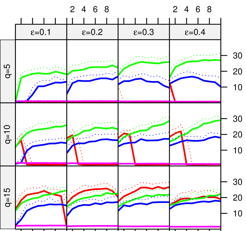
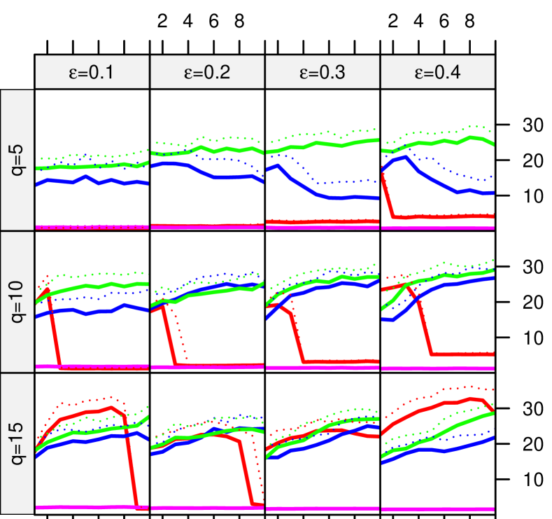
Figure 1: $\mbox{bias}(\boldsymbol{V}_{q})$ for $p=100$, shift (top) and point-mass (bottom) as a function of $\nu$. ROBPCA, PcaPP, PcaL, FastHCS.

We next consider the high dimensional case of $p>n$. Figure 2. Across all scenarios, the results are comparable to those in seen in Figure 1. FastHCS is the best performing method, being unaffected by the outliers, while the other methods show high biases on most settings.

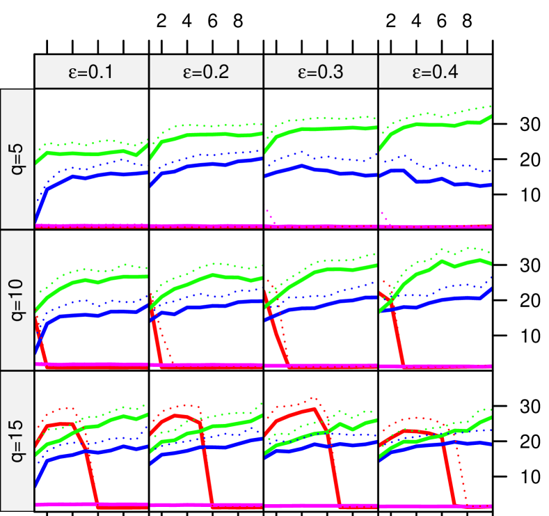
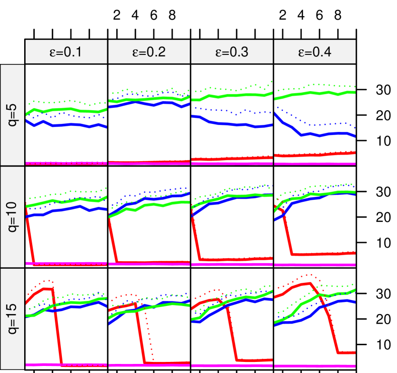
Figure 2: $\mbox{bias}(\boldsymbol{V}_{q})$ for $p=400$, shift (top) and point-mass (bottom) as a function of $\nu$. ROBPCA, PcaPP, PcaL, FastHCS.

Over all of the scenarios, FastHCS shows almost no bias, despite challenging outlier configurations. Furthermore, the bias curves corresponding to the fits found by FastHCS are also less variable: throughout, the 75th percentile of the bias corresponding to the FastHCS fit is typically closer to the median bias than is the case for the other algorithms. These findings indicate that FastHCS meets Criteria (4)-(5) for a robust PCA method. In contrast, we find that the performance of the other methods vary with the configuration of the outliers, the rate of the contamination, and the dimensionality of the $q$-subspace. In Section 5 of the Online Resources, we re-analyze these simulation results, giving similar plots for a measure of outlier misclassification, as well as the principal angle measure and $\mbox{bias}(\boldsymbol{P}_{q})$, two measures of quality of fit focusing on the loadings.

An extended simulation study shows that the results we present above are robust the choice of different simulation settings (for example, those used in (Maronna, 2005)), and different bias measurments criterions. However, since the outcome of the extended study is nearly identical to the one we present in this section, we have relegated these results in the Online Resources.

4 Real data applications

We next apply the algorithms to three real data examples. We selected these examples because in each the observations in the data can be separated into two subgroups from which we construct a majority and an outlier group. They are taken from three fields that regularly use PCA: character recognition, chemometrics and genetics. A feature shared by all of these data sets is that the variables within each are measured on the same scale. Data sets with this property were selected to remove the ancillary problem of data standardization. If the variables are not on the same scale, it is common practice in PCA modelling to standardize the data, but the choice of how to do so robustly adds a layer of subjectivity to the results. For the interested reader, the data sets used in this section are included in the FastHCS package. Section 6 of the Online Resources explains how the reader can use code we provide to replicate all results in this section.

The implementations of ROBPCA and PcaPP we use do not have an option to set the seed, but to ensure reproducibility of the results for FastHCS, we set seed=1. PcaL is a deterministic algorithm and uses no seeds. As in the simulations, we run each algorithm with default settings, except for the alpha parameter in ROBPCA which we set to 0.5. To illustrate the outlier detection capabilities of the algorithms, we display diagnostics plots. These show the $\operatorname*{OD}$ and $\operatorname*{SD}$ values for each observation, divided by the cut-off values in Equations (8) and (9) to put each of the methods on a comparable scale.

4.1 Selecting the number of components

We recommend using as large a value of $q$ as possible for FastHCS, since this improves its outlier detection performance. However, to avoid the curse of dimensionality, it is also advised to set $q<n/5$ (Hubert et al., 2005). In all the examples that follow, we select a relatively high number of components, $q=15$, to strike a balance between computation time and accuracy. Once the outliers have been detected, components with large eigenvales can be analyzed and used to construct a PCA model of the good data. One may also wish to use a selection criterion, such as the scree chart or contribution to variance. In Section 7 of the Online Resources, we also show results using the latter of these approaches in an extended analysis. In that analysis, the chemometrics data set illustrates how robust PCA methods parametrized based on a parsimonious, eigenvalue-based criterion, may miss outliers on minor components, even when the majority of the data may be modelled using a parsimonious model.

[capbesideposition=right,top,capbesidewidth=4cm]figure[]

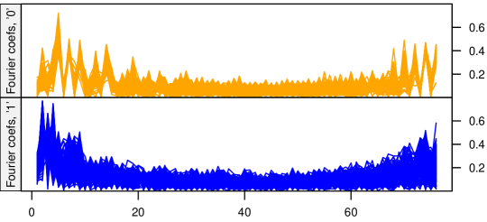
Figure 3: The 350 vectors of Fourier coefficients of the character shapes for the Multiple Features data set. The first 150 curves (corresponding to observations with labels ’0’) are show in the top panel in light orange. The Main group (200 curves) corresponding to observations with labels ’1’ are shown in the bottom panel.

[capbesideposition=right,top,capbesidewidth=4cm]figure[]

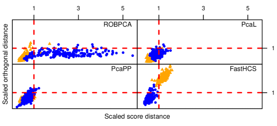
Figure 4: Diagnostic plots of the scaled score and orthogonal distances of the Fourier coefficients of the numerals for the robust PCA fits corresponding to the four algortihms for the Multiple feature data set. The observations corresponding to numerals with labels ’1’ (’0’) are shown as dark blue circles (light orange triangles).

[capbesideposition=right,top,capbesidewidth=4cm]figure[]

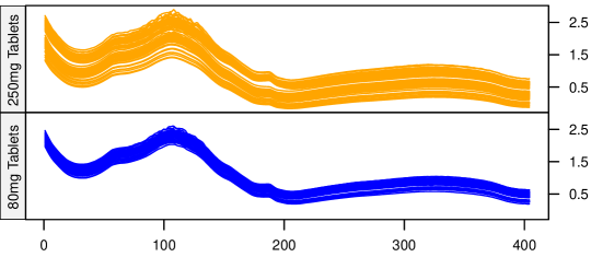
Figure 5: Spectra of fifty 250mg (light orange) tablets and eighty 80mg (dark blue) tablets for the Tablet data set.

[capbesideposition=right,top,capbesidewidth=4cm]figure[]

Figure 6: Diagnostic plots of the scaled score and orthogonal distances of the measured spectra corresponding to the four robust PCA fits for the Tablet data set. The observations corresponding to 80mg (250mg) tablets are shown as dark blue circles (light orange triangles).

[capbesideposition=right,top,capbesidewidth=4cm]figure[]

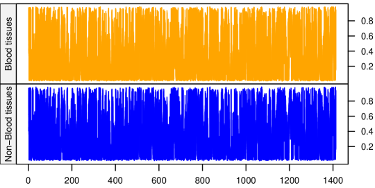
Figure 7: The 198 vectors of cytosine methylation $\beta$ values for the DNA alteration data set. The first 85 curves (corresponding to observations taken from blood tissues) are show in the top panel in light orange. The main group (113 curves) corresponding to observations taken from non-blood, tissues are shown in the bottom panel in dark blue.

[capbesideposition=right,top,capbesidewidth=4cm]figure[]

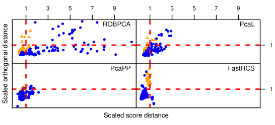
Figure 8: Diagnostic plots of the scaled score and orthogonal distances of cytosine methylation $\beta$ values corresponding to the four robust PCA algorithms for the DNA alteration data set. The observations with labels ”non-blood” (”blood”) are shown as dark blue circles (light orange triangles).

4.2 The Multiple Features data set

The Multiple Features data set (Van Breukelen et al., 1998) contains many replications of hand written numerals (’0’-’9’) extracted from nine original maps of a Dutch public utility. For each numeral, we have 200 replications (the observations) expressed as a vector of 76 of Fourier coefficients (the features) describing its shape. Finally, each numeral has been manually identified, yielding an extra vector of class labels. In this application, we will combine the vectors of Fourier coefficients corresponding to the 200 replications of the digit ’1’ to the vector of Fourier coefficients corresponding to the first 150 replications of the digit ’0’ (so that $n=350$ and $p=76$). The goal of the methods will be to distinguish the ’0’s and the ’1’s.

To give an impression of the differences between the two groups, we plot the Fourier coefficients corresponding to the main (outlier) subgroup in the bottom (top) panels of Figure 3 as dark blue (light orange) curves. In general, the curves corresponding to the members of the two groups are visually similar. In particular, the vertical ranges of both largely overlap, and both sets of curves exhibit a similar pattern of variance clustering where the central 40 Fourier coefficients have systematically less dispersion than higher or lower ones.

Figure 4 depicts the four resulting diagnostic plots. We assign to each observation a color (dark blue or light orange) and a plot symbol (round or triangle) depending on whether the corresponding curve describes a member of class ’1’ or ’0’, respectively. The outlier plots of PcaPP and PcaL show that neither method makes any distinction between the two digits, and observations from both groups influence the corresponding PCA models. ROBPCA discovers a different structure in the data, confounding the ’0’s as the majority group and the ’1’s as outliers on the model space. Since only a few ’1’s are $\operatorname*{OD}$ outliers, almost all of the observations influence the fitted loadings. In contrast to the other methods, FastHCS correctly identifies all of the ’0’s as outliers and identifies some ’1’s that might warrant additional scrutiny.

4.3 The Tablet data set

The Tablet data (Dyrby et al., 2002) contains the results of an analysis on Escitalopram${}^{\mbox{\scriptsize\textregistered}}$ tablets from the pharmaceutical company H. Lundbeck A/S using near-infrared (NIR) spectroscopy. The study includes tablets of four different dosages from pilot, laboratory and full scale production settings are included. Each tablet (the observations) is measured along 404 wavelengths (the variables). From this data, we extract two subsets of observations which we combine to obtain a new data set formed of two heterogeneous subgroups. Tablets of 80mg will make up the majority group and the rows corresponding to the first 50 tablets with a nominal weight of 250mg will serve as the outliers. This gives a high-dimensional data set (i.e. $p>n$) with $n=130$, $p=404$ and a contamination rate of $\varepsilon=38\%$.

Figure 5, depicts the spectra of the 250mg (light orange) and 80mg (dark blue) tablets. The spectra of the 250mg tablets follow a different multivariate pattern than those of the 80mg tablets. For example, the spectra of the former are generally lower and more spread out than the spectra of the latter. Dyrby et al. (2002) explain that accurate models for NIR analyses of medical tablets are valuable for quality control purposes, since they are fast, nondestructive, noninvasive, and require little preparation. The goal of the algorithms will be to fit a model to the 80mg tablets, despite the presence in the sample of many 250mg tablets.

Figure 6 depicts the diagnostic plots of the scaled outlyingness measures obtained from each of the algorithms. To enhance the distinction between the two groups in our data, we show the 80mg tablets as (dark) blue circles and the 250mg tablets as (light) orange triangles. These results are similar to those we saw when we examined the Multiple Features data set. Again PcaPP and PcaL do not distinguish between the two groups and ROBPCA uses both groups to fit the loadings parameters and confuses the outliers with the majority group on the model space. In contrast, the diagnostic plot derived from the FastHCS fit establishes that the 250mg tablets do not follow the same multivariate patterns as 80mg tablets and, in fact, depart significantly from it. In the plot, we see that FastHCS assigns the outliers high $\operatorname*{OD}$ values; excluding them from loadings and eigenvalue estimation. It also assigns many of them high $\operatorname*{SD}$ values; revealing their distance on the model space.

4.4 DNA Alteration data set

In our final case study, we examine another high-dimensional data set; the DNA Alteration data set (Christensen et al., 2009). This data set consists of cytosine methylation $\beta$ values collected at 1413 autosomal CpG loci (the variables) in a sample of 217 non-pathological human tissue specimens (the observations) taken from 10 different anatosites. In Christensen et al. (2009), the authors show that the tissue samples in this data set form three well separated subgroups. The first of these constitutes all 113 observations corresponding to cytosine methylation $\beta$ values measured on ”non-blood, non-placenta” (henceforth, simply ”non-blood”) tissues. A second subgroup of data points comprises the 85 cytosine methylation $\beta$ measurements taken on blood tissues.

In this application, we will combine the 113 measurements of cytosine methylation $\beta$ values corresponding to the samples ”non-blood” tissue with 85 measurements taken from blood tissues (so that $n=198$ and $p=1413$). In Figure 7, we plot the 1413 $\beta$ values corresponding to each blood (light orange) and non-blood (dark blue) observation. Visually, the curves of these two groups appear difficult to distinguish from one another. In particular, the vertical range of both overlap and the groups do not exhibit any pronounced difference in the variability of the variables.

The diagnostic plot for PcaPP (Figure 8) reveals that the fitted model regards blood and non-blood tissue to be quantitatively similar. ROBPCA and PcaL also detect almost none of the outliers, but additionally consider a number of the non-blood observations to be $\operatorname*{SD}$ outliers. As in the previous case studies, FastHCS correctly identifies all of the outliers. As a consequence, the parameter estimates corresponding to this model are more likely to reflect the true structure of non-blood tissue than those fitted by the other algorithms.

5 Outlook

In this article we introduced FastHCS to satisfy a number of criteria we expect a robust PCA method to have. In both the simulations and real data examples we performed, FastHCS met all of these criteria. In contrast, state-of-the-art methods did not, and often produced results one would expect from a non-robust method. This may seem like an extreme outcome, but it is in fact the very nature of dealing with outliers: if a method fails to identify them, the resulting model fit is often profoundly changed.

It is interesting to compare the performance of FastHCS and ROBPCA because these methods both use variants of projection pursuit. While FastHCS compares the fit produced by the $I$-index to that from the projection pursuit criterion, ROBPCA relies completely on the projection pursuit criterion to construct its initial subset. Thus, the difference in performance between FastHCS and ROBPCA that we observe in our simulations and real data examples arises from the fact that FastHCS nearly always chooses the $I$-index subset over the projection pursuit one.

In most applications, admittedly, data settings and contamination patterns will not be as difficult as those we featured in our simulations and real data examples, and in these easier cases the different methods will, hopefully, concur. Nevertheless, in three real data examples from fields where PCA is widely used, we were able to establish that real world situations can be challenging enough to push current state-of-the-art outlier detection procedures to their limits and beyond, justifying the development of better solutions. In any case, given that in practice we do not know the configuration of the outliers, as data analysts, we prefer to carry out our inferences while planning for the worst contingencies.

6 Acknowledgements

The authors wish to acknowledge the helpful comments from two anonymous referees and the editor which improved this paper.

Appendix A Vulnerability of the $I$-index to orthogonal outliers

Throughout this appendix, let $\boldsymbol{Y}$ be an $n\times p$ data matrix of uncontaminated observations drawn from a rank $q$ distribution $\mathscr{F}$, with $q$ and integer satisfying $2<q<\min(p,n)$. However, we do not observe $\boldsymbol{Y}$ but an $n\times p$ (potentially) corrupted data matrix $\boldsymbol{Y}^{\varepsilon}$ that consists of $g<n$ observations from $\boldsymbol{Y}$ and $c=n-g$ arbitrary values with $\varepsilon=c/n$ denoting the (unknown) rate of contamination. Throughout, $h=\lceil\left.(n+q+1)\middle/2\right.\rceil$ and the PCA estimates $(\boldsymbol{t}^{I},\boldsymbol{L}_{q}^{I},\boldsymbol{P}_{q}^{I})$ are defined as in Section (2) with $(\boldsymbol{L}_{q}^{I})_{j},1\leqslant j\leqslant q$ will denoting the $j$-th diagonal entry of $\boldsymbol{L}_{q}^{I}$.

We will consider the finite sample breakdown (Donoho, 1982) in the context of PCA following (Li and Chen, 1985):

$$\varepsilon_{1} = \min_{1\leqslant c\leqslant n}\{\varepsilon=\frac{c}{n}:(\boldsymbol{L}_{q})_{1}=\infty\}$$ (11)

$$\varepsilon_{2} = \min_{1\leqslant c\leqslant n}\{\varepsilon=\frac{c}{n}:(\boldsymbol{L}_{q})_{q}=0\}$$ (12)

Equation (11) defines the so-called finite sample explosion breakdown point and Equation (12) the so-called finite sample implosion breakdown point of PCA estimates $(\boldsymbol{t},\boldsymbol{L}_{q},\boldsymbol{P}_{q})$, and the general finite sample breakdown point is $\varepsilon^{*}_{n}=\min(\varepsilon_{1},\varepsilon_{2})$.

The following assumptions (as per, for example Tyler (1994)) all pertain to the original, uncontaminated, data set $\boldsymbol{Y}$. We will consider the case whereby the point cloud formed by $\boldsymbol{Y}$ lies in general position in $\mathbb{R}^{q}$. The following definition of general position is adapted from Rousseeuw and Leroy (1987):

Definition 1: General position in $\mathbb{R}^{q}$. $\boldsymbol{Y}$ is in general position in $\mathbb{R}^{q}$ if no more than $q$-points of $\boldsymbol{Y}$ lie in any $(q-1)$-dimensional affine subspace. For $q$-dimensional data, this means that there are no more than $q$ points of $\boldsymbol{Y}$ on any hyperplane, so that any $q+1$ points of $\boldsymbol{Y}$ always determine a $q$-simplex with non-zero determinant.

The $I$-index is shift invariant so that, w.l.o.g., we only consider cases where the good observations are centered at the origin. Throughout, we will also assume that the members of $\boldsymbol{Y}$ are bounded:

$$\max_{i=1}^{n}||\boldsymbol{y}_{i}||<U_{0}$$

for some bounded scalar $U_{0}$ depending only on the uncontaminated observations and that the uncontaminated observations contain no duplicates:

$$||\boldsymbol{y}_{i}-\boldsymbol{y}_{j}||>0\;\forall\;1\leqslant i<j\leqslant n.$$

A.1 Theorem 1: The implosion breakdown, $\varepsilon_{2}(\boldsymbol{t}^{I},\boldsymbol{L}_{q}^{I},\boldsymbol{P}_{q}^{I})$, is $\left.(n-h+1)\middle/n\right.$

Proof

If at least $h$ rows of $\boldsymbol{Y}^{\varepsilon}$ are in general position in $\mathbb{R}^{q}$, any subset of $h$ observations will contain at least $q+1$ observations in general position. This guarantees that the $q^{th}$ eigenvalue corresponding to any $h$-subset is non-zero (Seber, 2008). Thus, it follows that $\varepsilon_{2}(\boldsymbol{t}^{I},\boldsymbol{L}_{q}^{I},\boldsymbol{P}_{q}^{I})=\left.(n-h+1)\middle/n\right.$.

A.2 Finite sample explosion breakdown of $(\boldsymbol{t}^{I},\boldsymbol{L}_{q}^{I},\boldsymbol{P}_{q}^{I})$

Denote $\boldsymbol{z}\in\mathbb{R}^{p}$ the outlying entries of $\boldsymbol{Y}^{\varepsilon}$ and $\boldsymbol{z}^{m}=||\boldsymbol{z}\boldsymbol{P}_{0}^{m}||$. The only outliers capable of causing explosion breakdown must satisfy:

$$||\boldsymbol{z}|| \geqslant U_{1},$$ (13)

$$\min_{m}||\boldsymbol{z}\boldsymbol{P}_{0}^{m}|| \leqslant U_{2}.$$ (14)

for any bounded scalar $U_{1}$ and $U_{2}$ depending only on the uncontaminated observations.

Proof

Suppose that the outliers do not satisfy Equation (13) so that $\max_{i}||\boldsymbol{y}_{i}^{\varepsilon}||\leqslant U_{1}$, but that the PCA estimates $(\boldsymbol{t}^{I},\boldsymbol{L}_{q}^{I},\boldsymbol{P}_{q}^{I})$ break down. This leads to a contradiction since

$$(\boldsymbol{L}_{q}^{I})_{1}\leqslant\max_{i\in H^{I}}||\boldsymbol{y}_{i}^{\varepsilon}||$$ (15)

Therefore, for a contaminated $h$-subset to cause explosion breakdown, the outliers must satisfy Equation (13).

Assume that an outlier $\boldsymbol{z}$ does not satisfy Condition (14). Schmitt et al. (2014) showed that any $h$ subset $H^{m}$ indexing $\boldsymbol{z}$ will have an unbounded value of $I(H^{m},\boldsymbol{S}_{0}^{m})$ if and only if $\boldsymbol{z}^{m}$ is unbounded. But for the uncontaminated data, it holds that

$$\max_{i}\min_{m}||\boldsymbol{y}_{i}\boldsymbol{P}_{0}^{m}|| \leqslant U_{2}$$ (16)

so if the contaminated data set $\boldsymbol{Y}^{\varepsilon}$ contains at least $h$ entries from the original data matrix $\boldsymbol{Y}$, then it is always possible to construct a subset $H^{m}$ of entries of $\boldsymbol{Y}^{\varepsilon}$ for which $I(H^{l},\boldsymbol{S}_{0}^{l})$ is bounded so that $H^{m}$ will never be selected over $H^{l}$.

Appendix B The finite sample breakdown point of FastHCS

In this appendix, we derive the finite sample breakdown point of FastHCS. Define $\boldsymbol{Y}$, $\boldsymbol{Y}^{\varepsilon}$ and $\varepsilon^{*}_{n}$ as in Appendix A. Recall that

$$D(\boldsymbol{Y}^{\varepsilon},H^{I},H^{PP})=\operatorname*{ave}_{j=1}^{q}\log\frac{\operatorname*{ave}_{i\in H^{I}}((\boldsymbol{y}^{\varepsilon}_{i}-\boldsymbol{t}^{I})\boldsymbol{P}^{I}_{j})^{2}}{\operatorname*{var}_{i\in H^{\bullet}}(\boldsymbol{y}^{\varepsilon}_{i}\boldsymbol{P}^{I}_{j})}$$

$$-\max_{j=1}^{q}\log\frac{\operatorname*{ave}_{i\in H^{\bullet}}((\boldsymbol{y}^{\varepsilon}_{i}-\boldsymbol{t}^{PP})\boldsymbol{P}^{PP}_{j})^{2}}{\operatorname*{var}_{i\in H^{-}}(\boldsymbol{y}^{\varepsilon}_{i}\boldsymbol{P}^{PP}_{j})},$$ (17)

where $H^{-}=H^{PP}\setminus H^{I}$. Then, if $D(\boldsymbol{Y}^{\varepsilon},H^{I},H^{PP})>0$ or if $\displaystyle\max_{j=1}^{q}\operatorname*{var}_{i\in H^{-}}(\boldsymbol{y}^{\varepsilon}_{i}\boldsymbol{P}^{PP}_{j})=0$ then the final FastHCS estimates are based on $H^{PP}$. Otherwise, they are based on $H^{I}$.

Lemma 1

If $||\boldsymbol{y}^{\varepsilon}_{i}||>U_{1}$ and $\varepsilon<\left.(n-1)\middle/2n\right.$, then $i\notin H^{\bullet}$.

Proof

(Debruyne and Hubert, 2009) showed that the population breakdown point of $(\boldsymbol{t}^{PP},\boldsymbol{L}_{q}^{PP},\boldsymbol{P}_{q}^{PP})$ is 50%, which corresponds to a finite sample breakdown point of $\left.(n-1)\middle/2n\right.$. Consequently, $H^{PP}$ will not index any data point for which $||\boldsymbol{y}^{\varepsilon}_{i}||>U_{1}$. Since $H^{\bullet}$ indexes the overlap between $H^{I}$ and $H^{PP}$, if $||\boldsymbol{y}^{\varepsilon}_{i}||>U_{1}$, then $i\notin H^{\bullet}$.

Lemma 2

When $\boldsymbol{Y}$ is in general position, $n>q>2$, and $\varepsilon<\varepsilon_{1}=\left.(n-1)\middle/2n\right.,\;(\boldsymbol{L}_{q}^{I})_{1}<\infty$.

Proof

We will proceed by showing that the denominators in Equation (17) are bounded, while only the numerator dependent on $H^{PP}$ is bounded.

Lemma 1 implies there exists a fixed constant $U_{4}$ such that

$$||\boldsymbol{y}^{\varepsilon}_{i}\boldsymbol{P}_{j}||<U_{4}\;\forall\;i\in H^{\bullet},\;1\leqslant j\leqslant q$$ (18)

for any orthogonal matrix $\boldsymbol{P}$. Similarly, since the projection pursuit approach has a breakdown point of $\left.(n-1)\middle/2n\right.$, there exists a fixed $U_{5}$ such that

$$||\boldsymbol{y}^{\varepsilon}_{i}\boldsymbol{P}_{j}||<U_{5}\;\forall\;i\in H^{PP},\;1\leqslant j\leqslant q$$ (19)

As a consequence of (18) and (19), there exists a fixed constant $U_{6}$ such that:

$$\sum_{j}\log(\operatorname*{var}_{i\in H^{\bullet}}(\boldsymbol{y}^{\varepsilon}_{i}\boldsymbol{P}^{I}_{j})) < U_{6}$$ (20)

$$\sum_{j}\log(\operatorname*{var}_{i\in H^{-}}(\boldsymbol{y}^{\varepsilon}_{i}\boldsymbol{P}^{PP}_{j})) < U_{6}.$$

Next, note that

$$\max_{j}\log(\operatorname*{ave}_{i\in H^{I}}((\boldsymbol{y}^{\varepsilon}_{i}-\boldsymbol{t}^{I})\boldsymbol{P}^{I}_{j})^{2}) = (\boldsymbol{L}_{q}^{I})_{1}$$ (21)

$$\min_{j}\log(\operatorname*{ave}_{i\in H^{I}}((\boldsymbol{y}^{\varepsilon}_{i}-\boldsymbol{t}^{I})\boldsymbol{P}^{I}_{j})^{2}) = (\boldsymbol{L}_{q}^{I})_{q}\geqslant\epsilon>0,$$ (22)

(Equation (22) follows from Appendix A, Theorem 1), so that

$$\sum_{j}\log(\operatorname*{ave}_{i\in H^{I}}((\boldsymbol{y}^{\varepsilon}_{i}-\boldsymbol{t}^{I})\boldsymbol{P}^{I}_{j})^{2})$$ (23)

is not bounded from above. Conversely, $(\boldsymbol{t}^{PP},\boldsymbol{L}_{q}^{PP},\boldsymbol{P}_{q}^{PP})$ has an explosion breakdown point of $\left.(n-1)\middle/2n\right.$, so that there exists a fixed $U_{8}$ such that:

$$\sum_{j}\log(\operatorname*{ave}_{i\in H^{\bullet}}((\boldsymbol{y}^{\varepsilon}_{i}-\boldsymbol{t}^{PP})\boldsymbol{P}^{PP}_{j})^{2})<U_{8}.$$ (24)

From Equations (20) and the unboundedness of (23) it follows that the left-hand side in Equation (17) is unbounded. However, by Equations (20) and (24), the right-hand side of Equation (17) is bounded from above so that in cases where outliers cause explosion breakdown of $(\boldsymbol{t}^{I},\boldsymbol{L}_{q}^{I},\boldsymbol{P}_{q}^{I})$, criterion (17) will select $H^{*}=H^{PP}$. Since the breakdown point of $(\boldsymbol{t}^{PP},\boldsymbol{L}_{q}^{PP},\boldsymbol{P}_{q}^{PP})$ is $\left.(n-1)\middle/2n\right.$, we have that $\varepsilon_{1}=\left.(n-1)\middle/2n\right.$.

Lemma 3

When $\boldsymbol{Y}$ is in general position, $n>q>2$, and $\varepsilon<\varepsilon_{2}=(n-h+1)/n$, then $(\boldsymbol{L}_{q}^{I})_{q}>0$.

Proof

By Appendix A, Theorem 1, we have that the implosion breakdown point of $(\boldsymbol{t}^{I},\boldsymbol{L}_{q}^{I},\boldsymbol{P}_{q}^{I})$ is $\left.(n-h+1)\middle/n\right.$. The implosion breakdown point of $(\boldsymbol{t}^{PP},\boldsymbol{L}_{q}^{PP},\boldsymbol{P}_{q}^{PP})$ is $\left.(n-1)\middle/2n\right.$, which is higher, so it follows that $\varepsilon_{2}=\left.(n-h+1)\middle/n\right.$.

Theorem B.1

For $n>p+1>2$, the finite sample breakdown point of $\boldsymbol{L}_{q}$ is

$$\varepsilon_{n}^{*}(\boldsymbol{L}_{q},\boldsymbol{Y}^{\varepsilon})=\left.(n-h+1)\middle/n\right..$$

Proof

The finite sample breakdown point of $\boldsymbol{L}_{q}=\min(\varepsilon_{1},\varepsilon_{2})$. Given Lemmas 2 and 3, $\min(\left.(n-1)\middle/2n\right.,(n-h+1)/n)=(n-h+1)/n$.

Appendix C Measures of dissimilarity for robust PCA fits.

The objective of the simulation studies in Section 3.3 is to measure how much the fitted PCA parameters $(\boldsymbol{t},\boldsymbol{L}_{q},\boldsymbol{P}_{q})$ obtained by four robust PCA methods deviate from the true $(\boldsymbol{\mu}^{u},\boldsymbol{\Lambda}_{q}^{u},\boldsymbol{\Pi}_{q}^{u})$ when they are exposed to outliers. One way to compare PCA fits is with respect to their eigenvectors, as in the maxsub criterion (Björck and Golub, 1973):

$$\text{maxsub}(\boldsymbol{P}_{q})=\text{arccos}(\lambda_{q}^{\left.1\middle/2\right.}(\boldsymbol{D}_{q})),$$

where $\lambda_{q}(\boldsymbol{D}_{q})$ is the smallest eigenvalue of the matrix $\boldsymbol{D}_{q}=\boldsymbol{\Pi}_{q}^{\top}\boldsymbol{P}_{q}\boldsymbol{P}_{q}^{\top}\boldsymbol{\Pi}_{q}$. The maxsub has an appealing geometrical interpretation as it represents the maximum angle between a vector in $\boldsymbol{\Pi}_{q}$ and the vector most parallel to it in $\boldsymbol{P}_{q}$. However, it does not exhaustively account for the dissimilarity between two sets of eigenvectors. As an alternative to the maxsub, Krzanowski (1979) proposes the total dissimilarity:

$$\text{sumsub}(\boldsymbol{P}_{q})=\sum_{j=1}^{q}\lambda_{j}(\boldsymbol{D}_{q}),$$ (25)

which is an exhaustive measure of dissimilarity for orthogonal matrices. Furthermore, because $\sum_{j=1}^{q}\lambda_{j}(\boldsymbol{D}_{q})=\operatorname{Tr}(\boldsymbol{D}_{q})$ and $|\boldsymbol{D}_{q}|=1$ (Krzanowski, 1979), it is readily seen that (25) is a measure of sphericity of $\boldsymbol{D}_{q}$ (it is proportional to the likelihood ratio test statistics for non-sphericity of $\boldsymbol{D}_{q}$ (Muirhead, 1982, p. 333-335)). However, note that (25) now forfeits the geometric interpretation enjoyed by the maxsub.

In any case, measures of dissimilarity based solely on eigenvectors, such as the maxsub or sumsub, necessarily fail to account for bias in the estimation of the eigenvalues. This is problematic when used to evaluate robust fits because it is possible for outliers to exert substantially more influence on $\boldsymbol{L}_{q}$ than on $\boldsymbol{P}_{q}$. An extreme example is given by the so-called good leverage type of contamination in which the outliers lie on the subspace spanned by $\boldsymbol{\Pi}_{q}$ so that even the classical PCA estimate (whose eigenvalues can be made arbitrarely bad by such outliers) will have low values of $\text{maxsub}(\boldsymbol{P}_{q})$.

In contrast, we are interested in an exhaustive measure of dissimilarity; one that summarizes the the effects of the outliers on all the parameters of the PCA fit into a single number, so that the algorithms can be ranked in terms total dissimilarity. To construct such a measure, it is logical to base it on $\boldsymbol{\varSigma}_{q}^{u}=\boldsymbol{\Pi}_{q}^{u}\boldsymbol{\Lambda}_{q}^{u}(\boldsymbol{\Pi}_{q}^{u})^{\top}$ and its estimate $\boldsymbol{V}_{q}=\boldsymbol{P}_{q}\boldsymbol{L}_{q}\boldsymbol{P}_{q}^{\top}$ because they contain all the parameters of the fitted model. For our purposes, one need to only consider the effects of outliers on $\boldsymbol{G}_{q}=|\boldsymbol{V}_{q}|^{-1/q}\boldsymbol{V}_{q}$, the shape component of $\boldsymbol{V}_{q}$ (Hubert et al., 2014). This is because to rank the observations in a contaminated sample in terms of their true outlyingness (and thus reveal the outliers), it is sufficient to estimate the shape component of $\boldsymbol{\varSigma}_{q}^{u}$ correctly. Consequently, an exhaustive measure of dissimilarity between $\boldsymbol{G}_{q}$ and $\boldsymbol{\Gamma}_{q}=|\boldsymbol{\varSigma}_{q}|^{-1/q}\boldsymbol{\varSigma}_{q}$ is given by $\phi((\boldsymbol{\Gamma}^{u}_{q})^{-1/2}\boldsymbol{G}_{q}(\boldsymbol{\Gamma}^{u}_{q})^{-1/2})$, where $\phi$ is any measure of non-sphericity of its argument. In practice several choices of $\phi$ are possible, the simplest being the condition number of $\boldsymbol{W}$ which is defined as the ratio of the largest to the smallest eigenvalue of $\boldsymbol{W}$ (Maronna and Yohai, 1995), explaining the definition of $\text{bias}(\boldsymbol{V}_{q})$.

References

- Björck and Golub (1973) Björck, Å. and Golub, G. H. (1973). Numerical Methods for Computing Angles Between Linear Subspaces. Mathematics of Computation, 27, 2, 579–594.
- Christensen et al. (2009) Christensen, B.C Houseman, E.A. Marsit, C.J. Zheng, S. Wrench, M.R. Wiemels, J.L. Nelson, H.H. Karagas, M.R. Padbury, J.F. Bueno, R. Sugarbaker, D.J Yeh, R., Wiencke, J.K. Kelsey, K.T. (2009). Aging and Environemental Exposure Alter Tissue-Specific DNA Methylation Dependent upon CpG Island Context. PLoS Genetics 5(8), e1000602.
- Croux and Ruiz-Gazen (2005) Croux, C. and Ruiz-Gazen, A. (2005). High breakdown estimators for principal components: the projection-pursuit approach revisited. Journal of Multivariate Analysis, 95, 206–226.
- Donoho (1982) Donoho, D.L. (1982). Breakdown properties of multivariate location estimators. Ph.D. Qualifying Paper Harvard University.