Abstract

In this paper we give a formula for the probability that $n$ random points chosen under the uniform distribution in a disk are in convex position. While close, the formula is recursive and is totally explicit only for the first values of $n$.
Mathematics Subject Classification (2000) Primary 52A22; 60D05
Key Words:Random convex chain, random polygon, exact distribution, Sylvester’s problem, geometrical probability

Part of this work is supported by ANR blanc PRESAGE (ANR-11-BS02-003)

1 Introduction

All the random variables are assumed to be defined on a common probability space $(\Omega,{\cal A},`P)$. The expectation is denoted by $`E$. The plane will be sometimes viewed as $`R^{2}$ or as $\mathbb{C}$ and we will pass from the real notation (e.g. $(x,y)$) to the complex one $(\rho e^{i\theta})$ without any warning. For a set $A$ in $`R^{2}$, $|A|$ denotes the Lebesgue measure of $A$. We denote by $\partial B$ the border of a set $B$. For any $n\geq 1$, any $z$, notation $z[n]$ stands for the $n$ tuple $(z_{1},\dots,z_{n})$ and $z\{n\}$ for the set $\{z_{1},\dots,z_{n}\}$. For $H$ be a compact convex domain in $`R^{2}$ with non empty interior, for any $n\geq 0$, $`P_{H}^{n}$ denotes the law of $n$ i.i.d. points $z[n]$ taken under the uniform distribution over $H$. A $n$-tuple of points ${\sf x}[n]$ of the plane is said to be in convex position if the $x_{i}$’s all belong to $\partial{\sf ConvexHull}({\sf x}\{n\})$. Further we define

$${\sf CP}_{n,m}=\big{\{}{\sf x}[n]:\#\{i~{}:~{}x_{i}\in\partial{\sf ConvexHull}({\sf x}\{n\})\}=m\big{\}}$$

the set of $n$ tuples ${\sf x}[n]$ for which exactly $m$ are on the border of $\partial{\sf ConvexHull}({\sf x}\{n\})$. Hence ${\sf CP}_{n}:={\sf CP}_{n,n}$ is the set of $n$-tuples of points in convex position. Finally, we let

$$P^{n}_{H} = `P_{H}^{n}(z[n]\in{\sf CP}_{n}),$$ (1)

$$P^{n,m}_{H} = `P_{H}^{n}(z[n]\in{\sf CP}_{n,m}).$$ (2)

The aim of the paper is to establish a formula for $P_{D}^{n}$, the probability that $n$ i.i.d. random points taken under the uniform distribution in a disk $D$ are in convex position; we will also compute $P_{D}^{n,m}$ the probability that exactly $m$ points among these $n$ points are on $\partial{\sf ConvexHull}({\sf z}\{n\})$. To compute $P_{D}^{n}$ we need and obtain a result more general than the disk case only, result about for what we will call bi-pointed segments (${\sf BSEG}$). This will play somehow the role of the bi-pointed triangle (see (15)) as studied by Bárány & al [3], central also in the approach of Buchta [6] (see (16)) of the computation of $P^{n,m}_{T}$ and $P^{n,m}_{S}$ (where $T$ stands for triangle, and $S$ for square).

For $\theta\in[0,2\pi]$, $R>0$, the arc of circle ${\sf AC}(\theta,R)$ is defined by

$${\sf AC}(\theta,R)=\{Re^{i\nu},\nu\in[-\theta/2,\theta/2]\}.$$

Figure 1: Representation of typical ${\sf SEG}(\theta,R)$ for $0<\theta<\pi$ and $\pi<\theta<2\pi$

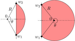
We denote by ${\sf SEG}(\theta,R)$ the segment (SEG) corresponding to the convex hull of ${\sf AC}(\theta,R)$ (see Fig. 1). Now consider $w_{1}(\theta,R)=Re^{-i\theta/2}$ and $w_{2}(\theta,R)=Re^{i\theta/2}$ the two extremities of the special border $[w_{1}(\theta,R),w_{2}(\theta,R)]$ of ${\sf SEG}(\theta,R)$. Let $z_{1},\dots,z_{n}$ be i.i.d. and uniform in ${\sf SEG}(\theta,R)$. Set

$$Z[n,\theta,R]=\{w_{1}(\theta,R),w_{2}(\theta,R),z_{1},\dots,z_{n}\},$$

and define the crucial bi-pointed segment case (${\sf BSEG}$) function

$$B_{n,m}(\theta):=`P(Z[n,\theta,R]\in{\sf CP}_{n+2,m+2}),~{}~{}~{}\theta\in(0,2\pi),1\leq m\leq n.$$ (3)

The value of $R$ has no importance since there exists a dilatation sending ${\sf SEG}(\theta,R)$ on ${\sf SEG}(\theta,R^{\prime})$, and dilatations conserve convex bodies and uniform distribution. But it will be useful to have the two parameters $(\theta,R)$ for subsequent computations. Again, we write $B_{n}$ instead of $B_{n,n}$ and below $L_{n}$ instead of $L_{n,n}$. Clearly, for any $\theta\in(0,2\pi)$, $B_{0}(\theta)=B_{1}(\theta)=1$. Now for any $n\geq 0$, $\theta\in(0,2\pi)$ define

$$L_{n,m}(\theta) = \frac{B_{n,m}(\theta)(\theta-\sin(\theta))^{n}\sin(\theta/2)}{n!}$$ (4)

Hence

$$L_{0}(\theta)=\sin(\theta/2),~{}~{}~{}L_{1}(\theta)=\sin(\theta/2)(\theta-\sin(\theta)).$$ (5)

Notice that $0$ (corresponding to the flat case) as well as $2\pi$ (the circle case) are excluded from definitions (3) and (4). The main contribution of this paper is the following theorem which allows to compute $P_{D}^{n,m}$.

Theorem 1

• For any $n\geq 1,$

  $$P_{D}^{n}=\lim_{t\to 2\pi\atop{t<2\pi}}B_{n-1}(t).$$

• For any $n\geq 2$,

  $$P_{D}^{n} = \frac{(n-2)!}{2^{n-2}\pi^{n-1}}\int_{0}^{2\pi}\sum_{k=0}^{n-2}L_{k}(\phi)L_{n-2-k}(2\pi-\phi)d\phi$$

• For any $\theta\in(0,2\pi)$, any $n\geq 1$,

  $$\frac{L_{n}(\theta)}{2}=\int_{0}^{\theta}\frac{\sin(\theta/2)^{2n+1}}{\sin(\phi/2)^{2n+1}}\int_{0}^{\phi}\sum_{k=0}^{n-1}L_{k}(\eta)L_{n-1-k}(\phi-\eta)d\eta d\phi.$$ (6)

  Analogous results can be obtained for $P_{D}^{n,m}$:

• For any $\theta\in(0,2\pi)$, for any $k,l\geq k+1$, $L_{k,l}(\theta)=0$. For any $\theta\in(0,2\pi)$, any $n\geq 1$ and $1\leq m\leq n$

  $$\frac{L_{n,m}(\theta)}{2} = \int_{0}^{\theta}\int_{0}^{\phi}\frac{\sin(\theta/2)^{2n+1}}{\sin(\phi/2)^{2n+1}}\sum_{n_{1}+n_{2}+n_{3}=n-1\atop{m_{1}+m_{2}=m-1}}\frac{(\sin(\eta)+\sin(\phi-\eta)-\sin(\phi))^{n_{3}}}{n_{3}!}$$

  $$\times L_{n_{1},m_{1}}(\eta)L_{n_{2},m_{2}}(\phi-\eta)d\eta d\phi$$

  An alternative form can be given using

  $$\sin(\eta)+\sin(\phi-\eta)-\sin(\phi) = 4\sin(\frac{\phi-\eta}{2})\sin(\phi/2)\sin(\eta/2).$$

• For any $n\geq 2$, $1\leq m\leq n$

  $$P_{D}^{n,m} = \frac{(n-2)!}{2^{n-2}\pi^{n-1}}\int_{0}^{2\pi}\sum_{n_{1}+n_{2}=n-1\atop{m_{1}+m_{2}=m-1}}L_{n_{1},m_{1}}(\phi)L_{n_{2},m_{2}}(2\pi-\phi)d\phi.$$

• For any $n\geq 1,$

  $$P_{D}^{n,m}=\lim_{t\to 2\pi\atop{t<2\pi}}B_{n-1,m-1}(t).$$

From $(ii)$, one can compute successively the $L_{j}(\theta)$, and by (4), this allows one to compute the $B_{n}(\theta)$. By $(i)$ it suffices then to take the limit when $\theta\to 2\pi^{-}$ (limit from below).

Despite important efforts we were not able to find a simpler formula for $B_{n}$ than that presented in the Theorem. Nevertheless, explicit computation can be done but close formula for the first $L_{j}$ given below shows a rapid growth of the complexity of the formula’s ($L_{10}$ would need one page to be written down). The effective computation of the first $L_{n}$ is complex and very few can be computed by hand. In particular the singularity apparent in (6) is difficult to handle since the terms in the sum needs to be combined to compensate the singularity.

In Section 3 we present an algorithm allowing one to compute the first terms of the sequence (using a computer, or years of time of an efficient human brain). With this algorithm I computed the 11 first values of $L_{n}$ which allows the computation $(P_{D}^{n},1\leq n\leq 12)$. $L_{0}$ and $L_{1}$ have been given in (5); the next ones are

$$L_{2}(\theta) = \frac{1}{6}\sin(\frac{\theta}{2})(3\theta^{2}+\sin(\theta)^{2}-16\sin(\frac{\theta}{2})^{2})$$

$$L_{3}(\theta) = {\frac{1}{54}}\,\sin(\frac{\theta}{2})\left(2\,\sin(\frac{\theta}{2})^{4}\sin(\theta)+9{\theta}^{3}+27\,\sin(\frac{\theta}{2})^{2}\theta+7\sin(\frac{\theta}{2})^{2}\sin(\theta)+105(\sin\left(\theta\right)-\theta)\right)$$

$$L_{4}(\theta) = {\frac{\sin(\frac{\theta}{2})}{12960}}\Big{(}160\,\sin(\frac{\theta}{2})^{6}+48\,\sin(\frac{\theta}{2})^{8}+60\,\sin(\frac{\theta}{2})^{4}+540\,{\theta}^{4}-13725\,{\theta}^{2}-7200\,\sin(\theta)\theta$$

$$+83700\,\sin(\frac{\theta}{2})^{2}\Big{)}$$

$$L_{5}(\theta) = {\frac{\sin(\frac{\theta}{2})}{1296000}}\Big{(}40500\sin(\theta){\theta}^{2}-584\sin(\frac{\theta}{2})^{4}\sin(\theta)+12000\sin(\frac{\theta}{2})^{4}\theta$$

$$-272\sin(\frac{\theta}{2})^{6}\sin(\theta)-549000{\theta}^{3}-2745000\sin(\frac{\theta}{2})^{2}\theta$$

$$+44270\sin(\frac{\theta}{2})^{2}\sin(\theta)+7102095(\theta-\sin(\theta))-64\sin(\frac{\theta}{2})^{8}\sin(\theta)+10800{\theta}^{5}\Big{)}$$

The next formula are too large to be written here. We can compute also $L_{m,n}(\theta)$ for small values of $m,n$. For any $n\geq 2$, $\sum_{k=1}^{n}B_{n,k}(\theta)=1$. Since $B_{2,2}=B_{2}$ is know, so do $B_{2,1}$. The next ones are

$$L_{3,1}(\theta) = -\frac{1}{6}\sin(\frac{\theta}{2})^{3}\Big{(}48\sin(\frac{\theta}{2})^{5}\cos(\frac{\theta}{2})-48\,\sin(\frac{\theta}{2})^{6}-12\sin(\frac{\theta}{2})^{3}\cos(\frac{\theta}{2})+8\sin(\frac{\theta}{2})^{4}$$

$$+12\sin(\frac{\theta}{2})^{2}\theta-10\cos(\frac{\theta}{2})\sin(\frac{\theta}{2})+40\sin(\frac{\theta}{2})^{2}-15\theta\Big{)}$$

$$L_{4,1}(\theta) = -\frac{1}{45}\sin(\frac{\theta}{2})^{4}\Big{(}48\sin(\frac{\theta}{2})^{4}\cos(\frac{\theta}{2})\theta-48\sin(\frac{\theta}{2})^{5}\theta-12\sin(\frac{\theta}{2})^{5}-12\,\cos(\frac{\theta}{2})\sin(\frac{\theta}{2})^{2}\theta$$

$$-48\sin(\frac{\theta}{2})^{3}\theta+190\sin(\frac{\theta}{2})^{3}+9\cos(\frac{\theta}{2})\theta+96\sin(\frac{\theta}{2})\theta-210\sin(\frac{\theta}{2})\Big{)}$$

the next ones are too large again, to be written here. I am able to compute $L_{n,m}$ for $n\leq 5$ (which provides the values of $P_{D}^{n,m}$ for $n\leq 7$).

Using these formulae, one finds the following explicit cute values for $P_{D}^{n}$

$$\begin{array}[]{|c|c|c|c|c|c|}\hline\cr n&4&5&6&7&8\\ \hline\cr 1-P_{D}^{n}&\frac{35}{12\pi^{2}}&\frac{305}{48\pi^{2}}&\frac{146400\pi^{2}-473473}{11520\pi^{4}}&\frac{512400\pi^{2}-2900611}{23040\pi^{4}}&\frac{62664108221+1721664000\,{\pi}^{4}-18670881600\,{\pi}^{2}}{48384000\pi^{6}}\\ \hline\cr\end{array}$$ (9)

By Theorem 1, we can also compute $P^{4,3}_{D}=\frac{35}{12\pi^{2}}$ (or by $P_{D}^{4,4}+P_{D}^{4,3}=1$), $P_{D}^{5,5}$ is given in the array, $P^{5,4}_{D}=\frac{65}{12\pi^{2}}$, $P^{5,3}_{D}=\frac{15}{16\pi^{2}}$, $P_{D}^{6,5}=\frac{3120\pi^{2}-17017}{288\pi^{4}}$, $P_{D}^{6,4}=\frac{7200\pi^{2}+57057}{3840\pi^{4}}$, $P_{D}^{6,3}=\frac{1001}{320\pi^{4}}$.

Explicit results for bi-pointed half disk ($B_{1}(\theta)=1$ for any $\theta\in(0,2\pi)$:

$$\begin{array}[]{|c|c|c|c|c|c|}\hline\cr n&2&3&4&5&6\\ \hline\cr 1-B_{n}(\pi)&\frac{16}{3\pi^{2}}&\frac{26}{3\pi^{2}}&\frac{-83968+13725\,{\pi}^{2}}{540\pi^{4}}&\frac{-97091+12200\,{\pi}^{2}}{240\pi^{4}}&\frac{30749622272-4885982325\,{\pi}^{2}+201757500\,{\pi}^{4}}{2268000{\pi}^{6}}\\ \hline\cr\end{array}$$ (12)

The only simple formula which appears is the following:

$$\lim_{t\to 0}B_{n}(t)=\frac{12^{n}}{(n+1)(2n+1)!}.$$

which holds for all $1\leq n\leq 11$. It corresponds to the limit for ${\sf BSEG}$ with an angle going to 0.

Apart the results exposed in Theorem 1, the only explicit results in the literature concerns triangles and parallelogram (we here discuss only results known for any $n$, in 2D). Valtr [13] (1995) has obtained that if $S$ is a square (or a (non flat) parallelogram) then, for $n\geq 1$,

$$P_{S}^{n}=\left(\frac{\binom{2n-2}{n-1}}{n!}\right)^{2},$$ (13)

and in a second paper, [14] (1996) he proved that if $T$ is a (non flat) triangle then, for $n\geq 1$,

$$P_{T}^{n}=\frac{2^{n}(3n-3)!}{(n-1)!^{3}(2n)!}.$$ (14)

Buchta [6] goes further and gives an expression for $P_{S}^{n,m}$ and $P_{P}^{n,m}$ as a finite sum of explicit terms.

For the bi-pointed triangle, Bárány, Rote, Steiger, Zhang [3] (2000) have shown the following. Let $T=(A,B,C)$ be a (non flat) triangle, and let $(z_{1},\dots,z_{n})$ be $`P_{T}^{n}$ distributed, and let $\overline{{\sf z}[n]}=(A,B,z_{1},\dots,z_{n})$ be the $n+2$ tuple obtained by adding $A,B$ to ${\sf z}[n]$. For any $n\geq 0$,

$$`P_{T}^{n}(\overline{{\sf z}[n]}\in{\sf CP}_{n+2})=\frac{2^{n}}{n!(n+1)!}.$$ (15)

These results are at the origin of numerous works concerning limit shape for convex bodies in a domain ([3], Bárány [1]) and for the evaluation of the probability that $n$ points chosen in a convex domain $H$ are in convex position (see Bárány [1]).

Buchta (2007) [5] goes forward and prove the following result : For any $n\geq 1$, any $1\leq m\leq n$,

$$`P_{T}^{n}(\overline{{\sf z}[n]}\in{\sf CP}_{n+2,m+2})=\sum_{C\in{\sf Comp}(n,m)}2^{m}\prod_{i=1}^{m}\frac{C_{i}}{SC_{i}(1+SC_{i})}$$ (16)

where $SC_{i}=C_{1}+\dots+C_{i}$ and ${\sf Comp}(n,m)$ is the set of compositions of $n$ in $m$ non empty parts (Examples : ${\sf Comp}(2,3)=\varnothing$, ${\sf Comp}(4,2)=\{(1,3),(3,1),(2,2)\}$).

Additional references

The literature concerning the question of the number of points on the convex hull for i.i.d. random points taken in a convex domain is huge. I won’t make a survey here but rather sends the interested reader to Reitzner [11], Hug [9] and to the various paper cited in the present paper I will focus on what concerns the disk.

Blaschke (1917) [4] proves that for the 4 points problem (the so-called problem of Sylvester), we have for any convex $K$,

$$P_{T}^{4}\leq P_{K}^{4}\leq P_{D}^{4}.$$

Bárány (2000) [1] have shown that

$$\lim_{n\to+\infty}n^{2}(P_{K}^{n})^{1/n}=e^{2}A^{3}(K)/4$$ (17)

where $A^{3}(K)$ is the supremum of the affine perimeter of all convex sets $S\subset K$. For the disk one gets

$$\log(P_{K}^{n})=-2n\log n+n\log\left(2\pi^{2}e^{2}\right)-2`e_{0}(3\pi^{4}n)^{1/5}+...$$ (18)

where the last term, not really proved in the mathematical sense, has been obtained by Hilhorst & al. [8]. Central limit theorems exists also for the number of points on $\partial{\sf ConvexHull}({\sf x}\{n\})$ under $`P_{D}^{n}$ (and for more general domain, under the uniform or Poisson distribution), see Groeneboom [7], Pardon [10], Bárány and Reitzner [2].

2 Proof of Theorem 1

2.1 Proof of $(i)$

All along this section $n\geq 1$ is fixed. Take a closed disk $\overline{B}=\overline{B}((0,0),R_{c})$, with center $(0,0)$ and radius $R_{c}={1}/{\sqrt{\pi}}$, that is with area 1, and pick $n$ i.i.d. uniform points $U_{1},\dots,U_{n}$ in $\overline{B}$. Now consider the smallest disk $\overline{B}((0,0),R_{n})$ that contains all the $U_{i}$’s. Clearly

$$R_{n}=\inf\{r:\#(\overline{B}(0,r)\cap\{U_{1},\dots,U_{n}\}\})=n\}.$$

Proposition 2

Conditionally on $R_{n}=r$, there is a.s. exactly one index $J\in\llbracket 1,n\rrbracket$ such that $U_{J}$ belongs to the circle ${B}((0,0),r)$. Conditionally on $\{J=j,R_{n}=r\}$, $U_{j}$ and $(U_{1},\dots,U_{j-1},U_{j+1},\dots,U_{n})$ are independent, $U_{j}$ has the uniform law on the circle $\partial B((0,0),r)$, and $U_{1},\dots,U_{j-1},U_{j+1},\dots,U_{n}$ are uniform in $\overline{B}((0,0),r)$.

Proof. A.s. the points $U_{1},\dots,U_{n}$ are not on the same circle with center $(0,0)$, and by symmetry conditionally on $R_{n}=r$ and $J=j$, $U_{j}$ is uniform on $B((0,0),r)$. Now, conditionally on $R_{n}=r$ and $J=j$, each variable $U_{\ell}$ (for $\ell\neq j$) are just conditioned to satisfy $\|U_{\ell}\|_{2}\leq r$, and this conditioning conserves the uniform distribution.  $\Box$

Proof of Theorem 1$(i)$. Theorem 1$(i)$ is – or should be – intuitively obvious, taking into account Proposition 2. This Proposition says that the two following models $(a)$ and $(b)$:
– $(a)$ $n$ points i.i.d. uniform in a disk,
– $(b)$ one point uniform on the circle and, independently, $n-1$ i.i.d. uniform inside the disk
are equivalent with respect to the probability to be in convex position.
Now if we come back to the ${\sf BSEG}$ considerations, when $\theta\to 2\pi$, the points $w_{1}(R_{c},\theta)$ and $w_{2}(R_{c},\theta)$ become closer and closer, and the line passing by these points lets all the other points in one of the half plane it defines. It is intuitively clear that replacing $w_{1}(R_{c},\theta)$ and $w_{2}(R_{c},\theta)$ by a single point close to them (for example, at position $(-R_{c},0)$) will not dramatically change the model nor the probability to be in convex position. This is the essence of Theorem 1$(i)$.

For sake of completeness, let us give a formal proof. Take $R>0$ and consider the two sets $S(`e)={\sf SEG}(2\pi-`e,R)$ and $S={\sf SEG}(2\pi,R)=\overline{B}((0,0),R)$. These two sets are close for the Hausdorff topology when $`e$ is small. We always have $S(`e)\subset S$, and $|S\setminus S(`e)|$ goes to 0. This property implies that if we fix $`e^{\prime}>0$, for $`e$ small enough, for $z_{1},\dots,z_{n}$ chosen uniformly and independently under $`P_{S}$,

$$`P(\{z_{1},\dots,z_{n}\}\subset S(`e))\geq 1-`e^{\prime}.$$ (19)

Conditionally on the event $\Lambda_{`e}:=\big{\{}\{z_{1},\dots,z_{n}\}\subset S(`e)\big{\}}$, the $z_{i}$’s are i.i.d. uniform in $S(`e)$. Let $w_{1}(`e)=w_{1}(R_{c},2\pi-`e)$, $w_{2}(`e)=w_{2}(R_{c},2\pi-`e)$, $w=-R$.

We want to show that $`P((z_{1},\dots,z_{n},w_{1}^{`e},w_{2}^{`e})\in{\sf CP}_{n+2}|\Lambda_{`e})\to`P((z_{1},\dots,z_{n},w)\in{\sf CP}_{n+1})$. Consider the following sets (subsets of $S^{n}$):

$$E_{1}(`e) := \{(t_{1},\dots,t_{n})\in S(`e)~{}:(t_{1},\dots,t_{n},w_{1}(`e),w_{2}(`e))\in{\sf CP}_{n+2}\}$$

$$E_{2} := \{(t_{1},\dots,t_{n})\in S~{}:(t_{1},\dots,t_{n},w)\in{\sf CP}_{n+1}\}.$$

It suffices to prove that $|E_{1}(`e)|\mathrel{\mathop{\kern 0.0pt\to}\limits_{`e\to 0}}|E_{2}|$. First $E_{1}(`e)\subset E_{2}$ since if $(t_{1},\dots,t_{n},w_{1}(`e),w_{2}(`e))$ belongs to ${\sf CP}_{n+2}$ and since the segments $[w_{1}(`e),w]$ and $[w_{2}(`e),w]$ are chords, then $(z_{1},\dots,z_{n},w_{1}(`e),w_{2}(`e),w)$ is in ${\sf CP}_{n+3}$ from what we deduce that $E_{2}$ is in ${\sf CP}_{n+1}$.

To end the proof take $(t_{1},\dots,t_{n})\in E_{2}$. We show that when $`e$ is small enough, it is in $E_{1}(`e)$. More precisely, we will see that it is not the case only if the $t_{i}$ belongs to a null set (for Lebesgue measure). We assume that $n\geq 2$ since for $n=1$ the result is clear.

First, for $`e>0$ small enough, if the $t_{i}$’s are different and different to $-R$, all the $t_{i}$ belongs to $S(`e)$. Since $(t_{1},\dots,t_{n},w)\in{\sf CP}_{n+1}$ draw the convex polygon $p$ passing by these points, and relabel the $t_{i}^{\prime}$s as $t_{1}^{\star},\dots,t_{n}^{\star}$ clockwise around $p$ so that the neighbours of $w$ are $t^{\star}_{1}$ and $t^{\star}_{n}$. Again, up to null set, the angles $(w,t^{\star}_{1},t^{\star}_{2})$ and $(t^{\star}_{n-1},t^{\star}_{n},w)$ are not 0, and it appears clearly that for $`e$ small enough, $(t_{1},\dots,t_{n},w_{1}(`e),w_{2}(`e))\in{\sf CP}_{n+2}$. We then have $E_{2}=\cup_{`e}E_{1}(`e)$ and the $E_{1}(x)\cup E_{1}(x^{\prime})$ if $x^{\prime}<x$, so $|E_{1}(`e)|\to|E_{2}|$ when $`e$ goes to 0.  $\Box$.

2.2 Proof of $(ii)$

For any $\theta\in[0,2\pi],R>0$,

$$|{\sf SEG}(\theta,R)|:=\frac{R^{2}}{2}\left(\theta-\sin(\theta)\right)$$ (20)

and then for

$$R_{\theta}=\sqrt{\frac{2}{\theta-\sin(\theta)}},$$ (21)

the area $|{\sf SEG}(\theta,R_{\theta})|=1$. Denote more simply by ${\sf SEG}_{\theta}$ the segment ${\sf SEG}(\theta,R_{\theta})$ with unit area. The size $L_{\theta}$ of the special border $[w_{1}(\theta,R_{\theta}),w_{2}(\theta,R_{\theta})]$ for this segment is

$$L_{\theta}=2R_{\theta}\sin(\theta/2).$$ (22)

In this section we fix $\theta\in(0,2\pi)$ and search to express $B_{n}(\theta)$ with some combinations of $B_{j}(\nu)$, for $\nu<\theta$ and $j<n$. To get the decomposition we will “push the arc of circle” ${\sf AC}(\theta,R)$ inside ${\sf SEG}(\theta,R_{\theta})$ till it touches one of the $z_{i}$’s doing something similar to the Buchta’s method (for the computation of $P_{S}^{n}$ and $P_{T}^{n}$). Here it is a bit more complex: we need the arc of circle to stay an arc of circle during the operation in order to get a nice decomposition, and also we somehow need to keep the bi-pointed elements. The arc angle and radius will change during the operation. This will lead to a quadratic formula for $B_{n}$.

  

Figure 2: Representation of the family ${\cal F}_{\theta}$. The angle $\phi<\theta$ and ${\sf SEG}[\phi]\leq{\sf SEG}[\theta]$. The angles are taken at the center of the circle that defines the segments.

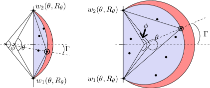
Almost of quantities appearing in this section should be indexed by $\theta$. In order to avoid heavy notation we won’t do this. Draw ${\sf SEG}_{\theta}$ in the plane. We consider the family of segments

$${\cal F}_{\theta}:=({\sf SEG}[\phi],0\leq\phi\leq\theta)$$

having as special border the special border of ${\sf SEG}_{\theta}$, that is $[w_{1}(\theta,R_{\theta}),w_{2}(\theta,R_{\theta})]$, and lying at its right, such that the angle of ${\sf SEG}[\phi]$ is $\phi$ (see Fig. 2).

When $\phi$ goes from $\theta$ to $0$, the center $O[\phi]$ of (the circle which defines) ${\sf SEG}[\phi]$ moves on the $x$-axis from $O[\theta]=0$ to $(-\infty,0)$. Comparing the distance from $O[\phi]$ to the special border, we can compute the coordinate of $O[\phi]$:

$$O[{\phi}]=\frac{L_{\theta}}{2}\left(\cot(\frac{\theta}{2})-\cot(\frac{\phi}{2})\right)$$ (23)

and the radius of ${\sf SEG}[\phi]$,

$$R[\phi]=R_{\theta}\frac{\sin(\theta/2)}{\sin(\phi/2)}.$$ (24)

Since the special border of all the ${\sf SEG}[\phi]$ is the same one sees that if $\phi<\phi^{\prime}$ then ${\sf SEG}[\phi]\subset{\sf SEG}[\phi^{\prime}]$. When $\phi$ goes to 0, ${\sf SEG}[\phi]$ goes to $[w_{1}(\theta,R_{\theta}),w_{2}(\theta,R_{\theta})]$ (for the Hausdorff topology). One also sees that ${\sf SEG}[\theta]={\sf SEG}_{\theta}$, and for $\phi<\theta$, by (20) and (21) ,

$$|{\sf SEG}[\phi]| = \left(\frac{\sin(\theta/2)}{\sin(\phi/2)}\right)^{2}\frac{\phi-\sin(\phi)}{\theta-\sin(\theta)}$$ (25)

and then the other segments of the family ${\cal F}_{\theta}$ have area smaller than 1 (see Fig. 2).

Again $\theta$ is fixed. Let $z_{1},\dots,z_{n}$ be $n\geq 1$ i.i.d. uniform random points in ${\sf SEG}_{\theta}$. Denote by

$$\Phi=\min\left\{\phi:\#(\{z_{1},\dots,z_{n}\}\cap{\sf SEG}[\phi]\right\})=n\},$$

and let $J$ the (a.s. unique) index of the variable $z_{j}$ on $\partial{\sf SEG}[\phi]$. Finally let $\Gamma$ be the (signed) angle $\big{(}(+\infty,0),O[\Phi],z_{J}\big{)}$ formed by the $x$-axis and the line $(0[\Theta],z_{J})$ (see Fig. 2). We have

Proposition 3

The distribution of $(\Phi,\Gamma)$ admits the following density $f_{(\Phi,\Gamma)}$ with respect to the Lebesgue measure

$$f_{(\Phi,\Gamma)}(\phi,\gamma)=n\,\frac{\sin(\theta/2)^{2n}}{(\theta-\sin(\theta))^{n}}\frac{(\phi-\sin(\phi))^{n-1}}{\sin(\phi/2)^{2n+1}}\left(\cos(\gamma)-\cos(\phi/2)\right)1_{0\leq\phi\leq\theta}\,1_{|\gamma|\leq\phi/2}.$$

Proof. First, the density of $z_{J}=(x,y)$ with respect to the Lebesgue measure on $|{\sf SEG}_{\theta}|$ is $ndxdy|{\sf SEG}_{x,y}|^{n-1}$ where $|{\sf SEG}_{x,y}|^{n-1}$ is the area of the unique element of the family ${\cal F}_{\theta}$ whose border contains $(x,y)$. We then just have to make a change of variables in this formula !

We search the unique pair $(\phi,\gamma)$ such that

$$x+iy=R[\phi]e^{i\gamma}+O[\phi].$$

Since by (25) and (23) everything is explicit, we can compute the Jacobian

$$\left|{\sf det}\left(\begin{array}[]{cc}\frac{\partial x}{\partial\phi}&\frac{\partial x}{\partial\gamma}\\ \frac{\partial y}{\partial\phi}&\frac{\partial y}{\partial\gamma}\end{array}\right)\right|=\frac{\sin(\theta/2)^{2}}{\sin(\phi/2)^{3}}\frac{(\cos(\gamma)-\cos(\phi/2))}{(\theta-\sin(\theta))}.$$

From what we deduce the wanted formula, using (25). $\Box$.

Now, it remains to end the decomposition of our problem. Conditionally on $(\Phi,\Gamma,J)=(\phi,\gamma,j)$, the points $z_{1},\dots,z_{j-1},z_{j+1},\dots,z_{n}$ are i.i.d. uniform in ${\sf SEG}[\phi]$.

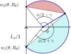
The triangle $T:=(w_{1}(\theta,R_{\theta}),w_{2}(\theta,R_{\theta}),z_{j})$ is inscribed in ${\sf SEG}[\phi]$ and ${\sf SEG}[\phi]\setminus T$ produces two segments $S_{1}$ and $S_{2}$. Since we may rescale ${\sf SEG}[\phi]$ to be ${\sf SEG}_{\phi}$ (to get area 1), the question now is that of the area of the two rescaled segments. After rescaling, $S_{1}$ and $S_{1}$ appear to be ${\sf SEG}[\phi/2+\gamma,R_{\phi}]$ and ${\sf SEG}[\phi/2+\gamma,R_{\phi}]$ since these lards have the right angles. Using (20)

$$|{\sf SEG}[\alpha,R_{\phi}]| = \frac{\alpha-\sin(\alpha)}{\phi-\sin(\phi)}.$$ (26)

We keep temporally notation $S_{1}$ and $S_{2}$ instead of ${\sf SEG}[\phi/2+\gamma,R_{\phi}]$ and ${\sf SEG}[\phi/2+\gamma,R_{\phi}]$ for short. The following Proposition is a simple consequence of the fact that the uniform distribution is conserved by conditioning. It is the “combinatorial decomposition” of the computation of $B_{n}(\theta)$, illustrated on Fig. 3.

Proposition 4

$(i)$ Conditionally on $(\Phi,\Gamma,J)=(\phi,\gamma,j)$, the respective number $(N_{1},N_{2},N_{3})$ of points of $z\{n\}\setminus\{z_{j}\}$ in $S_{1}$, $S_{2}$ and ${\sf SEG}_{\phi}-(S_{1}\cup S_{2})$ is

$${\sf Multinomial}(n-1,|S_{1}|,|S_{2}|,1-|S_{1}|-|S_{2}|).$$

$(ii)$ Conditionally on $(\Phi,\Gamma,J)=(\phi,\gamma,j)$ and $(N_{1},N_{2},N_{3})=(k_{1},k_{2},k_{3})$ the points $z_{1},\dots,z_{n}$ are in convex position with probability $1_{k_{3}=0,k_{1}+k_{2}=n-1}B_{k_{1}}(\phi/2+\gamma)B_{k_{2}}(\phi/2-\gamma)$.

Figure 3: Decomposition of the computation of $B_{n}(\theta)$, and definition of the two sub-segments appearing in the decomposition.

Putting everything together we have obtained

$$B_{n}(\theta) = \int_{0}^{\theta}\int_{-\frac{\phi}{2}}^{\frac{\phi}{2}}f_{(\Phi,\Gamma)}(\phi,\gamma)\sum_{k=0}^{n-1}\binom{n-1}{k}|S_{1}|^{k}|S_{2}|^{n-1-k}B_{k}(\phi/2+\gamma)B_{n-1-k}(\phi/2-\gamma)d\gamma d\phi$$

Set $\eta=\phi/2+\gamma$, $d\eta=d\gamma$, $\eta$ goes from $0$ to $\phi$ (and $\phi/2-\gamma=\phi-\eta$), giving

$$B_{n}(\theta) = \int_{0}^{\theta}\int_{0}^{\phi}f_{(\Phi,\Gamma)}(\phi,\eta-\phi/2)\sum_{k=0}^{n-1}\binom{n-1}{k}$$ (27)

$$\times |{\sf SEG}[\eta,R_{\phi}]|^{k}|{\sf SEG}[\phi-\eta,R_{\phi}]|^{n-1-k}B_{k}(\eta)B_{n-1-k}(\phi-\eta)d\eta d\phi$$ (28)

from which we get

$$B_{n}(\theta) = \int_{0}^{\theta}\int_{0}^{\phi}n\frac{\sin(\theta/2)^{2n}}{(\theta-\sin(\theta))^{n}}\frac{\cos(\eta-\phi/2)-\cos(\phi/2)}{\sin(\phi/2)^{2n+1}}\sum_{k=0}^{n-1}\binom{n-1}{k}$$ (29)

$$\times (\eta-\sin(\eta))^{k}B_{k}(\eta)((\phi-\eta)-\sin(\phi-\eta))^{n-1-k}B_{n-1-k}(\phi-\eta)d\eta d\phi.$$ (30)

Now, $\cos(\eta-\phi/2)-\cos(\phi/2)=2\sin(\eta/2)\sin((\phi-\eta)/2)$. Finally setting $L_{n}(\theta)$ as done in (4), we obtain Formula 1$(ii)$.

2.3 Proof $(i^{\prime})$

Recall Proposition 2. To compute $P_{n}^{D}$ we can work under the model where $n-1$ points $z_{1},\dots,z_{n-1}$ are picked independently and uniformly inside the disk $B((0,0),R_{c})$ (with $R_{c}=\pi^{-1/2}$) and one point on the border. We place this last point at position $-R_{c}$ which is allowed since rotation keeps convex bodies and the uniform distribution.

Now take a family of circles ${\cal G}=\{B[r],0\leq r\leq R_{c}\}$ such that $B[r]$ as radius $r$, its center at position $-R_{c}+r$, implying that $-R_{c}$ belongs to all these circles (see Fig. 4).

Figure 4: Decomposition of the computation of $P_{n}^{D}$. The big cross is the center of the initial circle, the small one, the center of the smallest circle containing all the points.

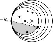
If $r^{\prime}<r$, $B[r^{\prime}]\subset B[r]$. Let $r^{\star}$ be the largest circle such that exists $1\leq k\leq n-1$, $z_{k}\in\partial B[r^{\star}]$. Denote then by $\phi$ the angle such that $z_{k}=(-R_{c}+r)+re^{i(-\pi+\phi)}$. If we denote by $(X,Y)$ the (Euclidean) position of $z_{k}$, the density of the distribution of $(x,y)$ is

$$(n-1)1_{(x,y)\in B((0,0),R_{c})}|B[r]|^{n-2}dxdy$$

where $B[r]$ is the unique circle in the family ${\cal G}$ which passes by $(x,y)$. We can then compute the Jacobian and find the distribution of $(r,\phi)$ to be with density $1_{0\leq r\leq R_{c},0\leq\phi\leq 2\pi}r(1-\cos(\phi))(\pi r^{2})^{n-2}drd\phi$. Once $z_{k}$ is given, we can once again normalise the problem, and come back on a circle of area $R_{c}$. We then get, using $1+\cos(\phi)=2\sin^{2}(\phi/2)$

$$P_{D}^{n} = (n-1)\int_{0}^{R_{c}}\int_{0}^{2\pi}\sum_{k=0}^{n-2}\binom{n-2}{k}2\sin^{2}(\phi/2)r(\pi r^{2})^{n-2}$$

$$\times B_{k}(\phi)B_{n-2-k}(2\pi-\phi)|{\sf SEG}(\phi,R_{c})|^{k}|{\sf SEG}(2\pi-\phi,R_{c})|^{n-2-k}d\phi dr$$

The integration with respect to $dr$ gives

$$P_{D}^{n} = \frac{1}{\pi}\int_{0}^{2\pi}\sum_{k=0}^{n-2}\binom{n-2}{k}\sin^{2}(\phi/2)B_{k}(\phi)B_{n-2-k}(2\pi-\phi)$$

$$\times \left(\frac{\phi-\sin(\phi)}{2\pi}\right)^{k}\left(\frac{2\pi-\phi+\sin(\phi)}{2\pi}\right)^{n-2-k}d\phi$$

since once $\phi$ is known, the convexity follows that on the pair of bi-pointed segments with angles $\phi$ and $2\pi-\phi$, and the number of elements in these segments is ${\sf binomial}\left(n-2,|{\sf SEG}(\phi,R_{c})|\right)$.

2.4 Proof of $(iii)$

The proof is the same as that of $(ii)$ except that in Proposition 4 we need to follow the number of points falling in the triangle. We then get

$$B_{n,m}(\theta) = \int_{0}^{\theta}\int_{0}^{\phi}f_{(\Phi,\Gamma)}(\phi,\eta-\phi/2)\sum_{n_{1}+n_{2}+n_{3}=n-1\atop{m_{1}+m_{2}=m-1}}\binom{n-1}{n_{1},n_{2},n_{3}}$$

$$\times |{\sf SEG}[\eta,R_{\phi}]|^{n_{1}}|{\sf SEG}[\phi-\eta,R_{\phi}]|^{n_{2}}(1-|{\sf SEG}[\eta,R_{\phi}]|-|{\sf SEG}[\phi-\eta,R_{\phi}]|)^{n_{3}}$$

$$\times B_{n_{1},m_{1}}(\eta)B_{n_{2},m_{2}}(\phi-\eta)d\eta d\phi$$

Using the notation introduced in (4) we get $(iii)$ .

2.5 Proof of $(iii^{\prime})$

Copy the arguments in Section 2.3. In the same way, for $n\geq 2$, $1\leq m\leq n$

$$P_{D}^{n,m} = \frac{1}{\pi}\int_{0}^{2\pi}\sum_{k=0}^{n-2}\sum_{1\leq m_{1}\leq n-2}\binom{n-2}{k}\sin^{2}(\phi/2)$$

$$\times B_{k,m_{1}}(\phi)B_{n-2-k,m-m_{1}-2}(2\pi-\phi)\left(\frac{\phi-\sin(\phi)}{2\pi}\right)^{k}\left(\frac{2\pi-\phi+\sin(\phi)}{2\pi}\right)^{n-2-k}d\phi$$

with the condition that $B_{k,k+l}=0$. $(iii^{\prime})$ follows.

2.6 Proof of $(iv)$

The same proof of $(i)$ does the job.

3 Effective computation of $L_{n}$

We explain in this part how to make effective computations. Since $B_{1}(\theta)=B_{0}(\theta)=1$, $L_{0}(\theta)$ and $L_{1}(\theta)$ are known by (4). Bruno Salvy [12] in a personal communication gave me a method to compute $B_{n}$ (my personal method fails at $n=7$).

Denote by $J_{n}(t)=\int_{0}^{t}\sum_{k=0}^{n-1}B_{k}(u)B_{n-1-k}(t-u)du$, and by $TJ_{n}$, $TB_{n}$ the Laplace transform of $J_{n}$ and $B_{n}$. We have

$$TJ_{n}(s)=\sum_{k=0}^{n-1}TB_{k}(s)TB_{n-k-1}(s).$$

It turns out that knowing the first values of $B_{k}$, the computation of $J_{n}$ by the previous formula and by inversion of the Laplace transform ends, using maple (when it does not by simple integration). Then it appears that $J_{n}(v)$ is a polynomial in $\sin(v),\cos(v)$ and $v$. The subsequent integration $\int_{0}^{t}J_{n}(v)/\sin(v)^{2n+1}dv$ is possible by helping the computer. Using $\cos(v)^{2}+\sin(v)^{2}=1$, it is possible to rewrite $J_{n}$ as polynomial of degree at most 1 in $\cos(v)$. Then write $J_{n}(v)/\sin(v)^{2n+1}$ under the form $Q_{0}+Q_{1}/\sin(v)^{1}+\sum_{l=1}^{2n+1}Q_{l}/\sin(v)^{l}$, where $Q_{n}$ is a polynomial in $\cos(v)$ and $v$. Then, proceed to successive integrations by parts, starting from the largest degree at the denominator till $l=2$. The remaining integral is computed by a simple integration.

This method allows one to compute 11 terms with maple. The computation of $B_{n,m}$ is possible using the same algorithm, except that some complications arise from the inverse Laplace which makes appear some polylogarithm functions (of the type ${\sf polylog}(n,e^{it})+{\sf polylog}(n,-e^{it}))$ for some $n\geq 2$). There limit at $t\to 0$ have to be treated separately, letting $\zeta(n)$ plays a role in the final result. I am able to compute $B_{n,m}$ for $n\leq 5$, and then $`P_{n,m}^{D}$ for $n\leq 7$.

References

- [1] I. Bárány. Sylvester’s question: The probability that n points are in convex position. Ann. Probab., 27(4):2020–2034, 1999.
- [2] I. Bárány and M. Reitzner. Poisson polytopes. The Annals of Probability, 38(4):1507–1531, 07 2010.
- [3] I. Bárány, G. Rote, W. Steiger, and C. Zhang. A central limit theorem for random convex chains. Discrete comput. Geom, 30:35–50, 2000.
- [4] W. Blaschke. Über affine geometrie xi: Lösung des ’vierpunktproblems’ von sylvester aus der theorie der geometrischen wahrscheinlichkeiten. Ber. Verh. Sachs. Akad. Wiss. Leipzig Math.-Phys, 69:436–453, 1917.
- [5] C. Buchta. The exact distribution of the number of vertices of a random convex chain. Mathematika, 53(2):247–254 (2007), 2006.
- [6] C. Buchta. On the number of vertices of the convex hull of random points in a square and a triangle. Anz. Österreich. Akad. Wiss. Math.-Natur. Kl., 143:3–10, 2009/10.
- [7] P. Groeneboom. Limit theorems for convex hulls. Probability Theory and Related Fields, 79(3):327–368, 1988.
- [8] H. Hilhorst, P. Calka, and G. Schehr. Sylvester’s question and the random acceleration process. Journal of Statistical Mechanics: Theory and Experiment, 2008(10):P10010, 2008.
- [9] D. Hug. Random polytopes. In Stochastic geometry, spatial statistics and random fields, volume 2068 of Lecture Notes in Math., pages 205–238. Springer, Heidelberg, 2013.
- [10] J. Pardon. Central limit theorems for uniform model random polygons. Journal of Theoretical Probability, 25(3):823–833, 2012.
- [11] M. Reitzner. New perspectives in stochastic geometry, Molchanov, I., and Kendall, W. edts, chapter Random polytopes (survey)., pages 45–76. Oxford University Press, Oxford., 2010.
- [12] B. Salvy. How to compute . Personal communication, 2013.
- [13] P. Valtr. Probability that n random points are in convex position. Discrete & Computational Geometry, 13:637–643, 1995.
- [14] P. Valtr. The probability that n random points in a triangle are in convex position. Combinatorica, 16(4):567–573, 1996.