In this paper we study the four point correlation function $\chi_{4}$ of collective density fluctuations in a nonequilibrium liquid. The equilibration is controlled by a modified stretched exponential behavior ( $\exp[-{(t_{\mathrm{w}}/\tau)}^{\beta}]$ ) having the relaxation time $\tau$ dependent on the aging time $t_{\mathrm{w}}$. Similar aging behavior has been seen experimentally in supercooled liquids. The basic equations of fluctuating nonlinear hydrodynamics (FNH) are solved here numerically to obtain $\chi_{4}$ for equilibrium and non equilibrium states. We also identify a dynamic length scale $\xi$ from the equilibrated function. $\xi(T)$ grows with fall of temperature $T$. From a broader perspective, we demonstrate here that the characteristic signatures of dynamical heterogeneities in a supercooled liquid, observed previously in computer simulations of the dynamics of a small number of particles, are also present in the coarse grained equations of generalized hydrodynamics.

Signatures of dynamic heterogeneity from a generalized hydrodynamic model of the supercooled liquid

A general feature emerging from simulationsonuki ; peter of the particle dynamics in a liquid is that at a given instant the atomic motions in different environments in the structurally disordered system evolve differently. And yet the fluid particles constantly move and rearrange so that the distinctions between different spatial environments of the fluid are transient. Understanding this complex and evolving situation, generally termed as dynamic heterogeneitiesediger is facilitated through the study of the multi particle correlation functions. The multi point structure of the correlation function is useful in probing the cooperative nature of the dynamics since it involves incorporating the information at two different spatial points corresponding to two different times simultaneously. In a number of recent works, a dynamic length scale franz-parisi ; sharon-par ; berth-fpt ; szammel depicting the strongly correlated nature of the supercooled liquid dynamics has been obtained analyzing a four point correlation functionchandan-epl . The different types of four point functions which have been studied in this respect involve some distinct property of the fluidjcp2 ; hca ; reich-imct ; flenner ; loidl1 like mobility or density of a tagged particle. In the present paper we study the dynamics in terms of that of the set $\{\rho({\bf x},t),{\bf g}({\bf x},t)\}$ respectively denoting the local densities of mass and momentum of the fluid. The nature of decay in the fluctuations of these conserved fields is also the focus of the microscopic theory, termed as as the mode coupling theory (MCT) for the slow dynamics in a supercooled liquid.

We compute the time dependent correlation function $\chi_{4}(q_{m},t)$ (to be defined below) involving the collective densities $\rho({\bf x},t)$ at four points. Here $q_{m}$ corresponds to the first maximum of structure factor. The four point function develops a sharp peak at a time $t=t_{\mathrm{p}}$ (say) and eventually decays out at larger times. The dynamic length $\xi(T)$, identified from analyzing cdg-PRL the four point function $\chi_{4}(q,t_{\mathrm{p}})$, grows roughly by a factor of three over the corresponding temperature range. The quantity $\chi_{0}\equiv\chi_{4}(0,t_{\mathrm{p}})$ grows as $\xi^{(2-\eta)}$ with the correlation length $\xi$ with the exponent $2-\eta=2.1$. In the non equilibrium state without time translation invariance kob_barrat , the four point function $\chi_{4}(t,t_{\mathrm{w}})$ for several different values of the waiting (aging) time $t_{\mathrm{w}}$, is seen to overlap in the $\alpha$-relaxation regime. The corresponding frequency transforms $\chi_{4}(\omega,t_{\mathrm{w}})$ collapse on a modified Kohlrausch-Williams-Watts (MKWW) relaxation curve relaxation time $\tau(t_{\mathrm{w}})$ dependent on $t_{\mathrm{w}}$. This is similar to the behavior seen in two point correlations Loidl ; bhaskar .

We consider the product $F(q;t,t_{\mathrm{w}})\equiv\delta\rho(q,t+t_{\mathrm{w}})\delta\rho(q,t_{\mathrm{w}})$ of the fourier transform of the density fluctuations $\delta\rho({\bf x},t)=\rho({\bf x},t)-\rho_{0}$ corresponding to wave vector $q$ at times $t+t_{\mathrm{w}}$ and $t_{\mathrm{w}}$ respectively. In the following $t_{\mathrm{w}}$ will be referred to as the waiting or aging time. The normalized two point function is the noise averaged quantity ${C}(q,t+t_{\mathrm{w}},t_{\mathrm{w}})={\langle}F(q;t,t_{\mathrm{w}}){\rangle}/{\langle}F(q,t_{\mathrm{w}},t_{\mathrm{w}}){\rangle}$. The long time limit of the equilibrium averaged quantity ${<F(q;t,0)>}_{\mathrm{eq}}\equiv{\cal C}(q,t)$ changes discontinuously at the ergodicity non-ergodicity (ENE) transition of the MCT. The four point function $\chi_{4}(q;t,t_{\mathrm{w}})$ normalized with respect to its initial value is defined as,

$$\chi_{4}(q;t,t_{\mathrm{w}})=\frac{\langle F(q;t,t_{\mathrm{w}})F(-q;t,t_{\mathrm{w}})\rangle}{{|F(q;0,0)|}^{2}}~{}~{}.$$ (1)

To calculate these time correlation functions we need the dynamical equations controlling the time evolution of density fluctuations in the liquid. The stochastic equations of fluctuating nonlinear hydrodynamics (FNH) for the coarse grained densities $\{\rho({\bf x},t),{\bf g}({\bf x},t)\}$ are written in the form :

$$\frac{\partial\rho}{\partial{t}}+{\bf\nabla}.{\bf g}=0,$$ (2)

$$\frac{\partial g_{i}}{\partial t}+v_{0}^{2}\{\nabla_{i}\rho-\rho\nabla_{i}f({\bf x},t)\}+L^{0}_{ij}\frac{g_{j}}{\rho}=\theta_{i},$$ (3)

where $v_{o}=1/\sqrt{\beta{m}}$ denotes the thermal speed at temperature $T$. Here $\theta_{i}$ denotes the thermal noise which is assumed to be gaussian and white. The noise correlation is related to the bare transport matrix $L^{0}_{ij}$ through the standard fluctuation dissipation relation. The function $f({\bf x},t)$ signify the role of interaction between the fluid particles and is obtained as a convolution function of the direct correlation function $c({\bf x})$ and the density fluctuation $\delta\rho({\bf x},t)$. Hence the fourier transform is obtained as $f(\textbf{k},t)=n_{0}c(\textbf{k})\delta\rho(\textbf{k},t)$ where $n_{0}$ is the equilibrium number density ($\rho_{0}=mn_{0}$). The slow dynamics of the MCT originates from a feedback mechanism caused by the density nonlinearities in the eqn. (3) of FNH. We have ignored the convective non linearities in the eqn. (3) to focus on the role of the coupling of density fluctuations.

The eqns. (2)-(3) of FNH are solved numerically on a cubic lattice of size $20$ with a grid length $h$. Two inputs are required here. First, the direct correlation function $c(r)$ related to the structure of the liquid input-sk . Second, the bare transport coefficients $L_{ij}^{0}$ defining the noise correlations are chosen such that the corresponding short time dynamics agrees with computer simulation data. We consider a system of $N$ particles, each of mass $m$ interacting via Lennard-Jones(LJ) potential of characteristic length scale $\sigma$. Time is scaled with $\tau_{0}=(m\sigma^{2}/\epsilon)^{\frac{1}{2}}$ and length with lattice constant $h$. The thermodynamic state of the fluid is described in terms of the reduced density $\rho^{*}=\rho_{0}\sigma^{3}$ and the reduced $T^{*}=(k_{B}T)/\epsilon$. The density fluctuations are saved in selected time bins. A whole array consisting of the density fluctuations $\rho({\bf x},t)$ on the cubic lattice ${\bf x}$ are transformed using fast fourier transform subroutines. From this data the two point and four point correlation functions are respectively obtained. Several runs for the dynamic evolution of the system driven by the noise is considered. Equilibrium is inferred when time translational invariance of the correlation function is observed, i.e., the two time correlation function $C(t_{\mathrm{w}},t+t_{\mathrm{w}})$ depends on $t$ only. This is attained at increasingly larger $t_{\mathrm{w}}$ as the liquid is further supercooled.

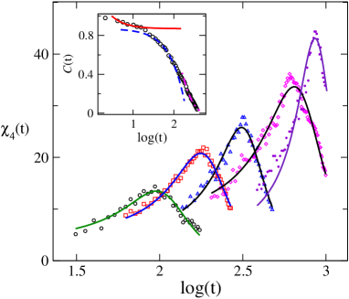
Figure 1: The normalized four point functions $\chi_{4}(t)$ at $q=q_{m}$ vs. time $t$ at ${\rho^{*}_{0}}=1.10$ and $T^{*}=1.0$(circles), $0.8$(squares), $0.7$(triangles), $0.6$(diamonds), $0.5$(stars). Solid lines are the best fit curves of Lorentzian form. Inset shows the two point function at ${\rho^{*}_{0}}=1.10$ and $T^{*}=0.8$. The solid and dashed curves indicate the respective power law fits predicted in MCT.

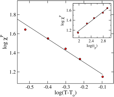
Figure 2: The peak $\chi^{P}$ of $\chi_{4}(t)$ at $t=t_{\mathrm{p}}$ appear to diverge around $T_{o}=0.2$ with exponent $\alpha=1.21$. Inset shows $\chi^{P}{\sim}t_{\mathrm{p}}^{\mu}$ behavior with the exponent $\mu=0.47$.

We equilibrated the system at average density $\rho^{*}_{0}=1.10$ and temperatures respectively at $T^{*}=1.0$, $0.8$, $0.7$, $0.6$ and $0.5$. For even lower temperatures $T^{*}=0.4$ the system does not equilibrate within the maximum time limit of computation time. The ratio of the two characteristic lengths $\sigma/h=4.6$ is kept fixed. The data for $\rho({\bf x},t)$ and ${\bf g}({\bf x},t)$ at each of the grid points are stored for times at equal intervals extending up to a maximum time $t_{\mathrm{max}}$ depending on the temperature $T^{*}$. For $T^{*}=.6$ we have $t_{\mathrm{max}}$ ($2000\tau_{0}$). To study the equilibrium correlation functions, we consider large enough initial times $t_{\mathrm{w}}$. Fig. 1 displays the four point function $\chi_{4}(t)$ obtained by evaluating RHS of eqn. (1) for $q=q_{m}$. From the same data for the $\rho({\bf x},t)$ the two point equilibrium correlation function $C(t+t_{\mathrm{w}},t_{\mathrm{w}})\equiv{\cal C}(t)$ is also obtained and shown in the inset of Fig. 1. The two point function ${\cal C}(t)$ reaches a small plateau value $f_{c}=0.87$ at $T^{*}=.8$. Following the predictions of MCT rmp the power law exponents $a$ and $b$ corresponding the power law and subsequent von-Sncheider relaxation are 1.27 and 1.18 respectively. For the four point function $\chi_{4}$ the peak height $\chi^{P}$ is attained at $t=t_{\mathrm{p}}$ which grows with supercooling indicating the growth of amorphous cluster size. We obtain $\chi^{P}\sim{(T-T_{o})}^{-1.2}$ with $T_{o}=.2$ as shown in Fig. 2. The growth of $t_{\mathrm{p}}$ observed with fall of $T$ is not as strong as that of the $\alpha$-relaxation time $\tau_{\alpha}$ over the same temperature change. The inset of Fig. 2 displays the dependence $\chi^{P}{\sim}t_{\mathrm{p}}^{\mu}$ with the exponent $\mu=0.47$.

The four point correlation function $\chi_{4}(q,t)$ obtained above is further analyzed to obtain the dynamic correlation length $\xi$. In Fig 3 we show the scaling of the peak height $\chi_{4}(q,t_{\mathrm{p}})\equiv\chi^{P}(q)$ for different values of wave vector $q$ using the Ornstein-Zernike form which includes the $O(q^{4})$ cdg-PNAS ; hca contribution. From the wave vector dependent data at a fixed $T$, the correlation length $\xi(T)$ is obtained . The inset (a) of Fig. 3 shows in the $\xi(T)$ vs. $T$ plot that the dynamic correlation length does not diverge around the so called MCT transition temperature $T_{c}$. By fitting the $\alpha$-relaxation time $\tau_{\alpha}$ to a power law divergence form we obtain $T_{c}=.4$ in the present casebhaskar of one component LJ system. The length $\xi(T)$ increases only by a factor of $3$ which is close to corresponding results seen in MD simulation of a binary LJ mixture jcp2 over a similar temperature range. In the inset (b) of Fig. 3, plot of the peak height $\chi_{0}\equiv\chi_{4}(q=0,T)$ vs. the correlation length $\xi$ shows that $\chi_{0}\sim\xi^{(2-\eta)}$ with $2-\eta=2.1$. The corresponding value of ($2-\eta$) from simulation of Ref.cdg-PRL is $2.2-2.4$. With a simplified form of the MCT model in terms of density only, summing a class of ladder diagrams for the four point functions biroli-EPL however obtains a different prediction $2-\eta=4$. A key observation from our computation of the two and the four point correlation functions, using the same density fluctuation data is that the temperature dependence of the relaxation time $\tau_{\alpha}(T)$ (obtained from ${\cal C}(t)$) differs qualitatively from that of the dynamic length scale $\xi(T)$ (obtained from $\chi_{4}(t)$). We observe that the $\tau_{\alpha}(T)$ tends to diverge around a relatively higher temperature ($T_{c}$) while the growth of $\xi(T)$ is appears at best to be linked to an underlying transition at $T_{g}$ or $T_{K}$adam-gibbs and not to the MCT transition at $T_{c}$.

To focus on the nonequilibrium dynamics we study the waiting time ($t_{\mathrm{w}}$) dependence of the four point function $\chi_{4}(t,t_{\mathrm{w}})$ defined in eqn. (1) for $t_{\mathrm{w}}=200,400,600,800,1000$. The $\chi_{4}(t)$ in each case grows to a peak of height $\chi^{P}(t_{\mathrm{w}})$ (say) at time $t=t_{\mathrm{p}}(t_{\mathrm{w}})$. This is shown in Fig. 4. The peak time $t_{\mathrm{p}}$ grows with $t_{\mathrm{w}}$ and reaches a maximum at an intermediate $t_{\mathrm{w}}$ before equilibrating for even longer waiting times as shown in the inset of Fig. 4. The peak height $\chi^{P}$ of the corresponding $\chi_{4}(t,t_{\mathrm{w}})$ increases with $t_{\mathrm{w}}$, signifying growing dynamic correlation. A parametric plot of $\chi_{4}(t,t_{\mathrm{w}})$ vs. $C(t,t_{\mathrm{w}})$ is useful for understanding the evolution of the two point and four point correlations in the non equilibrium system. The $\alpha$-relaxation parts of the $\chi_{4}(t,t_{\mathrm{w}})$ curves for different $t_{\mathrm{w}}$ overlapsriram-saroj with the corresponding two point function $C(t,t_{\mathrm{w}})$ being shifted by a $t$ independent part $f(t_{\mathrm{w}})$. We plot in Fig. 5 the $\chi_{4}(t,t_{\mathrm{w}})$ with respect to the quantity $\tilde{C}(t,t_{\mathrm{w}})=C(t,t_{\mathrm{w}})+f(t_{\mathrm{w}})$. The part $f(t_{\mathrm{w}})$ decays to zero as equilibrium is reached as shown in the inset of Fig. 5. We transform the $\chi_{4}(t,t_{\mathrm{w}})$ with respect to time $t$ to obtain $\chi_{4}(\omega,t_{\mathrm{w}})$ corresponding to frequencies given by $\omega{\tau_{0}}$=.0001,.0005,.001, and .01. The data for all $\omega$ values fit well to the form

$$\chi(\omega,t_{\mathrm{w}})=\left[\chi^{i}(\omega)-\chi^{f}(\omega)\right]g(t_{\mathrm{w}})+\chi^{f}(\omega),~{}~{}$$ (4)

where $\chi^{i}(\omega)$ and $\chi^{f}(\omega)$ respectively denote the initial and final values of the $\chi_{4}$ at the corresponding $\omega$. The relaxation function $g(t_{\mathrm{w}})$ has limiting values $1$ and $0$ respectively as $t_{\mathrm{w}}{\rightarrow}0$ and $\infty$. In the main Fig. 6 we show how the data for all frequencies at $T^{*}=.6$ collapse on a single curve (solid line) giving a frequency independent $g(t_{\mathrm{w}})$. The inset displays the $t_{\mathrm{w}}$ dependence of the relaxation time $\tau(t_{\mathrm{w}})$ characterizing the MKWW form of $g(t_{\mathrm{w}})$. The relaxation time $\tau(t_{\mathrm{w}})$ increases with $t_{\mathrm{w}}$ implying that aging slows down at longer waiting time $t_{\mathrm{w}}$. This is similar to the observed behaviorLoidl ; bhaskar with respect to the two point functions (dashed line in the main figure) obtained from experimental data. However for the four point functions the time $t_{\mathrm{w}}$ to reach saturation in $\tau(t_{\mathrm{w}})$ is much longer than that for two point case (see inset of Fig. 6).

We have demonstrated here that the appearance of a growing peak in the four point correlation function $\chi_{4}(t)$ is a general feature of the dynamics of the supercooled liquid and it follows from the basic equations of generalized hydrodynamics signifying conservation laws. This holds even if the two step process ( power law and von-Schneider law) predicted in the simple MCTrmp is not very clearly visible in the relaxation of two point correlation function ${\cal C}(t)$. Indeed for the simple LJ system considered here ${\cal C}(t)$ hardly shows any plateau so as to justify a two step relaxation process. The same density fluctuation data obtains the prominent peak in the four point function $\chi_{4}(t)$ growing with fall of temperature. At a quantitative level, however the the results for $\chi_{4}$ obtained from the present work differ from the predictions of a simplified MCT model which involves an ideal ENE transition. This is perhaps not unexpected given the fact that the oversimplified treatment of MCT gets modified in the extended MCTdas-mazenko when the implications of the $1/\rho$ nonlinearities are taken into account. From a wider perspective what is perhaps more relevantberth-garnier is that the general feature of dynamical heterogeneities follow from the basic equations of FNH which are also the starting point of the MCT. BSG acknowledges CSIR, India for financial support. SPD acknowledges support under grant 2011/37P/47/BRNS.

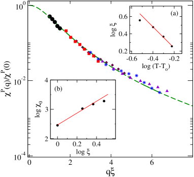
Figure 3: The normalized $\chi^{P}(q)/\chi^{P}(0)$ for density $\rho^{*}=1.10$ and different temperatures $T^{*}$=1.0(circles), 0.8(squares),0.7(diamonds),0.6(triangels), and 0.5 (stars) plotted with corresponding $q\xi(T)$. Dashed line is the best fit to an Ornstein-Zernike form (see text). Inset (a) shows divergence $\xi$ around the $T_{o}=0.2$ and exponent $1.4$. Inset (b) shows $\chi^{P}(q=0)\equiv{\chi_{0}}\sim\xi^{(2-\eta)}$ with $2-\eta=2.1$.

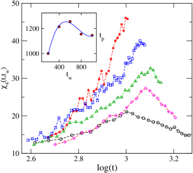
Figure 4: The non equilibrium $\chi_{4}(t,t_{\mathrm{w}})$ vs. $t$ for different values of the waiting time $t_{\mathrm{w}}$= 200(circles), 400(diamonds), 600(triangles), 800(squares), and 1000(stars) corresponding to $T^{*}$=0.4 and $\rho_{0}^{*}=1.1$. Inset : the peak time $t_{\mathrm{p}}$ vs. $t_{\mathrm{w}}$.

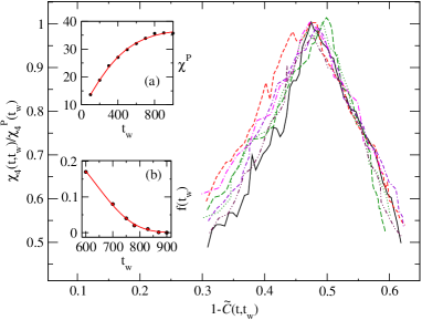
Figure 5: At $T^{*}=0.6$ and $\rho_{0}^{*}=1.1$, parametric plot of normalized $\chi_{4}(t,t_{\mathrm{w}})/\chi^{P}(t_{\mathrm{w}})$ vs. $1-\tilde{C}(t,t_{\mathrm{w}})$ (see text). Equilibration with waiting time $t_{\mathrm{w}}$ : Inset (a) the peak value $\chi^{P}$; (b) $f(t_{\mathrm{w}})$ (defined in text).

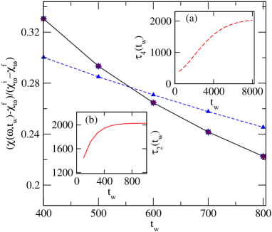
Figure 6: Data collapse (solid line) on the scaling function $g(t_{\mathrm{w}})$ (defined in the text) vs. $t_{\mathrm{w}}$ corresponding to four different frequencies $\omega\tau_{0}$== 0.0001(circle), 0.0005(diamond), 0.001(triangle), and 0.01(star) at $T^{*}=0.6$ and $\rho_{0}^{*}=1.1$. Scaling function corresponding to two point functions (dashed line). The $t_{\mathrm{w}}$ dependence of relaxation times of MKWW scaling functions: Inset (a) $\tau_{4}(t_{\mathrm{w}})$ for four point functions; Inset (b) $\tau_{2}(t_{\mathrm{w}})$ for two point functions.

References

- (1) R. Yamamoto and A. Onuki, J. Phys. Soc. Jpn. 66, 2545 (1997).
- (2) M. Hurley and P. Harrowell, Phys. Rev. E 52, 1694 (1995).
- (3) M. D. Ediger, Annu. Rev. Phys. Chem. 51, 99 (2000).
- (4) S. Franz and G. Parisi, J. Phys. Cond. Matt. 12 6335 (2000).
- (5) C. Donati, S. Franz, G. Parisi, SC Glotzer, J Non-Cryst Solids 307- 310, 215(2002).
- (6) L. Berthier, G. Biroli, J-P Bouchaud, L. Cipelletti, D. El. Masri, D. L’Hôte, F. Ladieu, and M. Pierno, Sceince,310, 1797 (2005).
- (7) G. Szamel, Phys. Rev. Lett. 101, 205701 (2008).
- (8) C. Dasgupta, A.V. Indrani, S. Ramaswamy, and M.K. Phani,Europhys. Lett. 15, 307 (1991).
- (9) Berthier L., G. Biroli, J-P Bouchaud, W. Kob, K. Miyazaki, and D. Reichman, 2007, J. Chem. Phys. 126, 184503 (2007); ibid J. Chem. Phys. 126, 184504(2007).
- (10) Richard S. L. Stein and Hans C. Andersen, Phys. Rev. Lett,101, 267802 (2008).
- (11) G. Biroli, J.-P. Bouchaud, K. Miyazaki, and D. R. Reichman, Phys. Rev. Lett. 97, 195701 (2006).
- (12) G. Szamel and E. Flenner, Phys. Rev. E 74, 021507 (2006).
- (13) T. Bauer, P. Lunkenheimer, A. Loidl, arXiv:1306.4630
- (14) S. P. Das, Rev. Mod. Phys. Rev. 76, 785 (2004).
- (15) S. Karmakara, C. Dasgupta, and S. Sastry, Phys. Rev. Lett. 105, 015701 (2010).
- (16) W. Kob and J.-L. Barrat, Phys. Rev. Lett. 78, 4581 (1997).
- (17) Lunkenheimer, R. Wehn, U. Schneider, and A. Loidl, Phys. Rev. Lett. 95, 055702 (2005).
- (18) B. Sen Gupta and S. P. Das, J. Chem. Phys. 136, 154506 (2012).
- (19) D. M. Due and A. D. J. Haymet, J. Chem. Phys. 103, 2625 (1995).
- (20) B. Sen Gupta, Shankar P. Das, and Jean-Louis Barrat, Phys. Rev. E 83, 041506(2011).
- (21) S. Karmakar, C. Dasgupta, and S. Sastry, Proc. Nat. Acad. Sci., 106, 3675 (2009).
- (22) G. Biroli, and J-P Bouchaud, Europhys. Lett., 67, 21 (2004).
- (23) G. Adam and J. H. Gibbs, J. Chem. Phys. 43, 139 (1965).
- (24) S. K. Nandi and S. Ramaswamy, Phys. Rev. Lett. 109, 115702 (2012); arxiv:1309.2389.
- (25) S. P. Das and G. F. Mazenko, Phys. Rev. A 34, 2265 (1986).
- (26) L. Berthier and J.P. Garrahan, Phys. Rev. E 68, 041201 (2003).