Regularization Parameter Estimation for Underdetermined problems by the $\chi^{2}$ principle with application to $2D$ focusing gravity inversion

Abstract

The $\chi^{2}$-principle generalizes the Morozov discrepancy principle to the augmented residual of the Tikhonov regularized least squares problem. For weighting of the data fidelity by a known Gaussian noise distribution on the measured data and, when the stabilizing, or regularization, term is considered to be weighted by unknown inverse covariance information on the model parameters, the minimum of the Tikhonov functional becomes a random variable that follows a $\chi^{2}$-distribution with $m+p-n$ degrees of freedom for the model matrix $G$ of size $m\times n$ and regularizer $L$ of size $p\times n$. Here it is proved that the result holds for the underdetermined case, $m<n$ provided that $m+p\geq n$ and that the null spaces of the operators do not intersect. A Newton root-finding algorithm is used to find the regularization parameter $\alpha$ which yields the optimal inverse covariance weighting in the case of a white noise assumption on the mapped model data. It is implemented for small-scale problems using the generalized singular value decomposition, or singular value decomposition when $L=I$. Numerical results verify the algorithm for the case of regularizers approximating zero to second order derivative approximations, contrasted with the methods of generalized cross validation and unbiased predictive risk estimation. The inversion of underdetermined $2D$ focusing gravity data produces models with non-smooth properties, for which typical implementations in this field use the iterative minimum support stabilizer and both regularizer and regularizing parameter are updated each iteration. For a simulated data set with noise, the regularization parameter estimation methods for underdetermined data sets are used in this iterative framework, also contrasted with the L-curve and the Morozov Discrepancy principle. These experiments demonstrate the efficiency and robustness of the $\chi^{2}$-principle in this context, moreover showing that the L-curve and Morozov Discrepancy Principle are outperformed in general by the three other techniques. Furthermore, the minimum support stabilizer is of general use for the $\chi^{2}$-principle when implemented without the desirable knowledge of a mean value of the model.

Keywords: Regularization parameter, $\chi^{2}$ principle, gravity inversion, minimum support stabilizer

1 Introduction

We discuss the solution of numerically ill-posed and underdetermined systems of equations, $\mathbf{d}=G\mathbf{m}$. Here $G\in\mathcal{R}^{m\times n}$, with $m<n$, is the matrix resulting from the discretization of a forward operator which maps from the parameter or model space to the data space, given respectively by the discretely sampled vectors $\mathbf{m}\in\mathcal{R}^{n}$, and $\mathbf{d}\in\mathcal{R}^{m}$. We assume that the measurements of the data $\mathbf{d}$ are error-contaminated, $\mathbf{d}_{\mathrm{obs}}=\mathbf{d}+\mathbf{n}$ for noise vector $\mathbf{n}$. Such problems often arise from the discretization of a Fredholm integral equation of the first kind, with a kernel possessing an exponentially decaying spectrum that is responsible for the ill-posedness of the problem. Extensive literature on the solution of such problems is available in standard literature, e.g. [1, 3, 8, 28, 31, 33].

A well-known approach for finding an acceptable solution to the ill-posed problem is to augment the data fidelity term, $\|W_{\mathbf{d}}(G\mathbf{m}-\mathbf{d}_{\mathrm{obs}})\|_{2}^{2}$, here measured in a weighted $L_{2}$ norm, by a stabilizing regularization term for the model parameters, $\|L(\mathbf{m}-\mathbf{m}_{0})\|_{2}^{2}$, yielding the Tikhonov objective function

$$P^{\alpha}(\mathbf{m}):=\|W_{\mathbf{d}}(G\mathbf{m}-\mathbf{d}_{\mathrm{obs}})\|_{2}^{2}+\alpha^{2}\|L(\mathbf{m}-\mathbf{m}_{0})\|_{2}^{2}.$$ (1)

Here $\alpha$ is the regularization parameter which trades-off between the two terms, $W_{\mathbf{d}}$ is a data weighting matrix, $\mathbf{m}_{0}$ is a given reference vector of a priori information for the model $\mathbf{m}$, and the choice of $L\in\mathcal{R}^{p\times n}$ impacts the basis for the solution $\mathbf{m}$. The Tikhonov regularized solution, dependent on $\alpha$, is given by

$$\mathbf{m}_{\mathrm{Tik}}(\alpha)=\textnormal{arg}\min_{\mathbf{m}}\{P^{\alpha}(\mathbf{m})\}.$$ (2)

If $C_{\mathbf{d}}=(W_{\mathbf{d}}^{T}W_{\mathbf{d}})^{-1}$ is the data covariance matrix, and we assume white noise for the mapped model parameters $L\mathbf{m}$ so that the model covariance matrix is $C_{L}=\sigma_{\mathrm{L}}^{2}I=\alpha^{-2}I=(W_{L}^{T}W_{L})^{-1}$, then (1) is

$$P^{\sigma_{\mathrm{L}}}(\mathbf{m})=\|G\mathbf{m}-\mathbf{d}_{\mathrm{obs}}\|_{C_{\mathbf{d}}^{-1}}^{2}+\|L(\mathbf{m}-\mathbf{m}_{0})\|_{C_{L}^{-1}}^{2}.$$ (3)

Note we will use in general the notation $\mathbf{y}\sim\mathbb{N}(\hat{\mathbf{y}},C_{\mathbf{y}})$ to indicate that $\mathbf{y}$ is normally distributed with mean $\hat{\mathbf{y}}$ and symmetric positive definite (SPD) covariance matrix $C_{\mathbf{y}}$. Using $C_{L}=\alpha^{-2}I$ in (3) permits an assumption of white noise in the estimation for $L\mathbf{m}$ and thus statistical interpretation of the regularization parameter $\alpha^{2}$ as the inverse of the white noise variance.

The determination of an optimal $\alpha$ is a topic of much previous research and includes methods such as the L-curve (LC) [7], generalized cross validation (GCV) [4], the unbiased predictive risk estimator (UPRE) [12, 29], the residual periodogram (RP) [10, 26], and the Morozov discrepancy principle (MDP) [18], all of which are well described in the literature, see e.g. [8, 31] for comparisons of the criteria and further references. The motivation and assumptions for these methods varies; while the UPRE requires that statistical information on the noise in the measurement data be provided, for the MDP it is sufficient to have an estimate of the overall error level in the data. More recently, a new approach based on the $\chi^{2}$ property of the functional (3) under statistical assumptions applied through $C_{L}$, was proposed by [13], for the overdetermined case $m>n$ with $p=n$. The extension to the case with $p\leq n$ and a discussion of effective numerical algorithms is given in [16, 22], with also consideration of the case when $\hat{\mathbf{m}}=\mathbf{m}_{\mathrm{0}}$ is not available. Extensions for nonlinear problems [15], inclusion of inequality constraints [17] and for multi parameter assumptions [14] have also been considered.

The fundamental premise of the $\chi^{2}$ principle for estimating $\sigma_{\mathrm{L}}$ is that provided the noise distribution on the measured data is available, through knowledge of $C_{\mathbf{d}}$, such that the weighting on the model and measured parameters is as in (3), and that the mean value $\hat{\mathbf{m}}$ is known, then $P^{\sigma_{\mathrm{L}}}(\mathbf{m}_{\mathrm{Tik}}(\sigma_{\mathrm{L}}))$ is a random variable following a $\chi^{2}$ distribution with $m+p-n$ degrees of freedom, $P^{\sigma_{\mathrm{L}}}(\mathbf{m}_{\mathrm{Tik}}(\sigma_{\mathrm{L}}))\sim\chi^{2}(m+p-n,c)$, with centrality parameter $c=0$. Thus the expected value satisfies $\hat{P}^{\sigma_{\mathrm{L}}}(\mathbf{m}_{\mathrm{Tik}}(\sigma_{\mathrm{L}}))=m+p-n$. As a result $P^{\sigma_{\mathrm{L}}}(\mathbf{m}_{\mathrm{Tik}}(\sigma_{\mathrm{L}}))$ lies within an interval centered around its expected value, which facilitates the development of the Newton root-finding algorithm for the optimal $\sigma_{\mathrm{L}}$ given in [16]. This algorithm has the advantage as compared to other techniques of being very fast for finding the unique $\sigma_{\mathrm{L}}$, provided the root exists, requiring generally no more than $10$ evaluations of $P^{\sigma_{\mathrm{L}}}(\mathbf{m}_{\mathrm{Tik}}(\sigma_{\mathrm{L}}))$ to converge to a reasonable estimate. The algorithm in [16] was presented for small scale problems in which one can use the singular value decomposition (SVD) [5] for matrix $G$ when $L=I$ or the generalized singular value decomposition (GSVD) [19] of the matrix pair $[W_{\mathbf{d}}G;L]$. For the large scale case an approach using the Golub-Kahan iterative bidiagonalization based on the LSQR algorithm [20, 21] was presented in [22] along with the extension of the algorithm for the non-central destribution of $P^{\sigma_{\mathrm{L}}}(\mathbf{m}_{\mathrm{Tik}}(\sigma_{\mathrm{L}}))$, namely when $\mathbf{m}_{\mathrm{0}}$ is unknown but may be estimated from a set of measurements. In this paper the $\chi^{2}$ principle is first extended to the estimation of $\sigma_{\mathrm{L}}$ for underdetermined problems, specifically for the central $\chi^{2}$ distribution with known $\mathbf{m}_{\mathrm{0}}$, with the proof of the result in Section 2 and examples in Section 2.4.

In many cases the smoothing that arises when the basis mapping operator $L$ approximates low order derivatives is unsuitable for handling material properties that vary over relatively short distances, such as in the inversion of gravity data produced by localized sources. A stabilizer that does not penalize sharp boundaries is instead preferable. This can be achieved by setting the regularization term in a different norm, as for example using the total variation, [24], already significantly studied and applied for geophysical inversion e.g. [23, 27]. Similarly,the minimum support (MS) and minimum gradient support (MGS) stabilizers provide solutions with non-smooth properties and were introduced for geophysical inversion in [25] and [33], respectively. We note now the relationship of the iterated MS stabilizer with non stationary iterated Tikhonov regularization, [6] in which the solution is iterated to convergence with a fixed operator $L$, but updated residual and iteration dependent $\alpha^{(k)}$ which is forced to zero geometrically. The technique was extended for example for image deblurring in [2] with $\alpha^{(k)}$ found using a version of the MDP and dependent on a good preconditioning approximation for the square model matrix. More generally, the iterative MS stabilizers, with both $L$ and $\alpha$ iteration dependent, are closely related to the iteratively reweighted norm (IRN) approximation for the Total Variation norm introduced and analyzed in [32]. In this paper the MS stabilizer is used to reconstruct non-smooth models for the geophysical problem of gravity data inversion with the updating regularization parameter found using the most often applied techniques of MDP and L-curve, contrasted with the UPRE, GCV and the $\chi^{2}$ principle. These results also show that the $\chi^{2}$ principle can be applied without knowledge of $\mathbf{m}_{\mathrm{0}}$ through the MS iterative process. Initialization with $\mathbf{m}_{\mathrm{0}}=0$ is contrasted with an initial stabilizing choice determined by the spectrum of the operator.

The outline of this paper is as follows. In Section 2 the theoretical development of the $\chi^{2}$ principle for the underdetermined problem is presented. We note that the proof is stronger than that used in the original literature when $m>n$ and hence improves the general result. The algorithm uses the GSVD (SVD) at each iteration and leads to a Newton-based algorithm for estimating the regularization parameter. A review of other standard techniques for parameter estimation is presented in Section 2.3 and numerical examples contrasting these with the $\chi^{2}$ approach also given, Section 2.4. The MS stabilizer is described in Section 3 and numerical experiments contrasting the impact of the choice of the regularization parameter within the MS algorithm for the problem of $2D$ gravity inversion in Section 3.1. Conclusions and future work are discussed in Section 4.

2 Theoretical Development

Although the proof of the result on the degrees of freedom for the underdetermined case $m<n$ effectively follows the ideas introduced [16, 22], the modification presented here provides a stronger result which can also strengthen the result for the overdetermined case, $m\geq n$.

2.1 $\chi^{2}$ distribution for the underdetermined case

We first assume that it is possible to solve the normal equations

$$(G^{T}W_{\mathbf{d}}^{T}W_{\mathbf{d}}G+L^{T}W_{L}^{T}W_{L}L)\mathbf{y}=G^{T}W_{\mathbf{d}}^{T}W_{\mathbf{d}}\mathbf{r},\,\,\mathbf{r}:=\mathbf{d}_{\mathrm{obs}}-G\mathbf{m}_{\mathrm{0}},\,\,\mathbf{y}=\mathbf{m}-\mathbf{m}_{\mathrm{0}}$$ (4)

for the shifted system associated with (3). The invertibility condition for (4) requires that $\tilde{L}:=W_{L}L$ and $\tilde{G}:=W_{\mathbf{d}}G$ have null spaces which do not intersect

$$\mathcal{N}(W_{L}L)\cap\mathcal{N}(W_{\mathbf{d}}G)=0.$$ (5)

Moreover, we also assume $m+p\geq n$ which is realistic when $L$ approximates a derivative operator of order $l$, then $p=n-l$, and typically $l$ is small, $n-l\geq 0$.

Following [16] we first find the functional $P^{W_{L}}(\mathbf{m}_{\mathrm{Tik}}(W_{L}))$ where $\mathbf{m}_{\mathrm{Tik}}(W_{L})=\mathbf{y}(W_{L})+\mathbf{m}_{\mathrm{0}}$ and $\mathbf{y}(W_{L})$ solves (4), for general $W_{L}$. There are many definitions for the GSVD in the literature, differing with respect to the ordering of the singular decomposition terms, but all effectively equivalent to the original GSVD introduced in [19]. For ease of presentation we introduce $\mathbf{1}_{k}$ and $\mathbf{0}_{k}$ to be the vectors of length $k$ with $1$, respectively $0$, in all rows, and define $q=n-m\geq 0$. We use the GSVD as stated in [1].

Lemma 1 (GSVD).

Suppose $H:=[\tilde{G};\tilde{L}]$, where $\tilde{G}$ has size $m\times n$, $m<n$, $\tilde{L}$ has size $p\times n$, $p\leq n$ with both $\tilde{G}$ and $\tilde{L}$ of full row rank $m$, and $p$, respectively, and by (5) that $H$ has full column rank $n$. The generalized singular value decomposition for $H$ is

$$[\tilde{G};\tilde{L}] =[U\tilde{\Upsilon}X^{T};V\tilde{M}X^{T}]$$ (6)

$$\tilde{\Upsilon}=\left[0_{m\times q}\ \ \Upsilon\right],\,\,\Upsilon =\mathrm{diag}(\nu_{q+1},\dots,\nu_{p},\mathbf{1}_{n-p})\in\mathcal{R}^{m\times m},\,\nu_{i}=1,i=p+1:n,$$ (7)

$$\tilde{M}=\left[M\ \ 0_{p\times(n-p)}\right],\,\,M =\mathrm{diag}(\mathbf{1}_{q},\mu_{q+1},\dots,\mu_{p})\in\mathcal{R}^{p\times p},\,\mu_{i}=1,i=1:q,$$ (8)

$$0<\nu_{q+1}\leq\dots\leq\nu_{p}<1, \quad 1>\mu_{q+1}\geq\dots\geq\mu_{p}>0,\quad\nu_{i}^{2}+\mu_{i}^{2}=1.$$ (9)

Matrices $U\in\mathcal{R}^{m\times m}$ and $V\in\mathcal{R}^{p\times p}$ are orthogonal, $U^{T}U=I_{m}$, $V^{T}V=I_{p}$, and $X\in\mathcal{R}^{n\times n}$ is invertible; $X^{-1}$ exists.

Remark 1.

The indexing in matrices $M$ and $\Upsilon$ uses the column index and we use the definitions $\mu_{i}=0$, $i=p+1:n$ and $\upsilon_{i}=0$, $i=1:q$. The generalized singular values are given by $\gamma_{i}=\upsilon_{i}/\mu_{i}$, $i=1:n$. Of these $n-p$ are infinite, $m+p-n$ are finite and non-zero, and $q$ are zero.

We first introduce $\tilde{\mathbf{r}}:=W_{\mathbf{d}}\mathbf{r}$ and note the relations

$$\tilde{\Upsilon}^{T}\tilde{\Upsilon} +\tilde{M}^{T}\tilde{M}=I_{n},\qquad\tilde{G}^{T}\tilde{G}+\tilde{L}^{T}\tilde{L}=XX^{T},\qquad\tilde{\Upsilon}\tilde{\Upsilon}^{T}=\Upsilon\Upsilon^{T},\qquad\mathrm{and}$$

$$\mathbf{y} =(X^{T})^{-1}\tilde{\Upsilon}^{T}U^{T}\tilde{\mathbf{r}},\qquad\tilde{G}\mathbf{y}=U\tilde{\Upsilon}\tilde{\Upsilon}^{T}U^{T}\tilde{\mathbf{r}},\qquad\tilde{L}\mathbf{y}=V\tilde{M}\tilde{\Upsilon}^{T}U^{T}\tilde{\mathbf{r}}.$$

Thus with $\mathbf{s}=U^{T}\tilde{\mathbf{r}}$, with indexing from $q+1:n$ for $\mathbf{s}$ of length $m$, $s_{i}=\mathbf{u}_{i-q}^{T}\tilde{\mathbf{r}}$,

$$P^{W_{L}}(\mathbf{m}_{\mathrm{Tik}}(W_{L})) =\tilde{\mathbf{r}}^{T}U(I_{m}-\tilde{\Upsilon}\tilde{\Upsilon}^{T})U^{T}\tilde{\mathbf{r}}=\sum_{i=q+1}^{p}\mu_{i}^{2}s_{i}^{2}=\|\mathbf{k}\|_{2}^{2},$$

$$\mathbf{k} =QU^{T}W_{\mathbf{d}}\mathbf{r},\quad Q:=\mathrm{diag}(\mu_{q+1},\dots,\mu_{p},\mathbf{0}_{n-p}).$$ (10)

To obtain our desired result on $P^{W_{L}}(\mathbf{m}_{\mathrm{Tik}}(W_{L}))$ as a random variable we investigate the statistical distribution of the components for $\mathbf{k}$, following [16, Theorem 3.1] and [22, Theorem 1] for the cases of a central, and non-central distribution, respectively, but with modified assumptions that lead to a stronger result.

Theorem 2.1 (central and non-central $\chi^{2}$ distribution of : $P^{W_{L}}(\mathbf{m}_{\mathrm{Tik}}(W_{L})$).

Suppose $\mathbf{n}\sim\mathbb{N}(0,C_{\mathbf{d}})$, $\mbox{\boldmath{$\zeta$}}:=(\mathbf{m}-\mathbf{m}_{\mathrm{0}})\sim\mathbb{N}(\hat{\mathbf{m}},C_{\mathbf{m}})$, $L\mbox{\boldmath{$\zeta$}}:=L(\mathbf{m}-\mathbf{m}_{\mathrm{0}})\sim\mathbb{N}(\hat{\mathbf{m}},C_{L})$, the invertibility condition (5), and that $m+p-n>0$ is sufficiently large that limiting distributions for the $\chi^{2}$ result hold. Then for

1. $\mathbf{m}_{\mathrm{0}}=\hat{\mathbf{m}}$: $P^{W_{L}}(\mathbf{m}_{\mathrm{Tik}}(W_{L}))\sim\chi^{2}(I_{m+p-n},0)$.

2. $\mathbf{m}_{\mathrm{0}}\neq\hat{\mathbf{m}}$: $P^{W_{L}}(\mathbf{m}_{\mathrm{Tik}}(W_{L}))\sim\chi^{2}({m+p-n},c)$, $c=\|QU^{T}W_{\mathbf{d}}G(\hat{\mathbf{m}}-\mathbf{m}_{\mathrm{0}})\|_{2}^{2}:=\|\mathbf{c}\|_{2}^{2}$.

Equivalently the minimum value of the functional $P^{W_{L}}(\mathbf{m}_{\mathrm{Tik}}(W_{L}))$ is a random variable which follows a $\chi^{2}$ distribution with $m+p-n$ degrees of freedom and centrality parameter $c=\|QU^{T}W_{\mathbf{d}}G(\hat{\mathbf{m}}-\mathbf{m}_{\mathrm{0}})\|_{2}^{2}$.

Proof.

By (10) it is sufficient to examine the components $k_{i}$, $i=q+1,\dots,p$ to demonstrate $\|\mathbf{k}\|^{2}$ is a sum of normally distributed components with mean $\mathbf{c}$ and then employ the limiting argument to yield the $\chi^{2}$ distribution, as in [16, 22]. First observe that $\mathbf{d}\sim\mathbb{N}(G\hat{\mathbf{m}},C_{\mathbf{d}}+GC_{\mathbf{m}}G^{T})$, thus $\mathbf{r}=\mathbf{d}_{\mathrm{obs}}-G\mathbf{m}_{\mathrm{0}}=\mathbf{d}+\mathbf{n}-G\mathbf{m}_{\mathrm{0}}=G(\mathbf{m}-\mathbf{m}_{\mathrm{0}})+\mathbf{n}\sim\mathbb{N}(G(\hat{\mathbf{m}}-\mathbf{m}_{\mathrm{0}}),C_{\mathbf{d}}+GC_{\mathbf{m}}G^{T})$, $W_{\mathbf{d}}\mathbf{r}\sim\mathbb{N}(W_{\mathbf{d}}G(\hat{\mathbf{m}}-\mathbf{m}_{\mathrm{0}}),W_{\mathbf{d}}(C_{\mathbf{d}}+GC_{\mathbf{m}}G^{T})W_{\mathbf{d}}^{T})$, and $\mathbf{k}\sim\mathbb{N}(QU^{T}W_{\mathbf{d}}G(\hat{\mathbf{m}}-\mathbf{m}_{\mathrm{0}}),QU^{T}W_{\mathbf{d}}(C_{\mathbf{d}}+GC_{\mathbf{m}}G^{T})W_{\mathbf{d}}^{T}UQ^{T})$. The result for the central parameter $c$ is thus immediate. For the covariance we have

$$C_{\mathbf{k}} =QU^{T}W_{\mathbf{d}}(C_{\mathbf{d}}+GC_{\mathbf{m}}G^{T})W_{\mathbf{d}}^{T}UQ^{T}=QQ^{T}+Q\tilde{\Upsilon}X^{T}C_{\mathbf{m}}X\tilde{\Upsilon}^{T}Q^{T}.$$ (11)

By assumption, $L$ has full row rank and $C_{\mathbf{m}}$ is SPD, thus for $C_{L}:=LC_{\mathbf{m}}L^{T}$ we can define $W_{L}:=\sqrt{C_{L}^{-1}}$. Therefore

$$I_{p}=W_{L}C_{L}W_{L}^{T}=W_{L}LC_{\mathbf{m}}L^{T}W_{L}^{T} =\tilde{L}C_{\mathbf{m}}\tilde{L}^{T}=V\tilde{M}X^{T}C_{\mathbf{m}}X\tilde{M}^{T}V^{T}\quad\mathrm{implies}$$

$$\tilde{M}(X^{T}C_{\mathbf{m}}X)\tilde{M}^{T} =I_{p}.$$ (12)

Introduce pseudoinverses for $\tilde{M}$ and $\tilde{M}^{T}$, denoted by superscript $\dagger$, and a dimensionally-consistent block decomposition for $(X^{T}C_{\mathbf{m}}X)$, in which $C_{11}$ is of size $p\times p$,

$$X^{T}C_{\mathbf{m}}X =\left(\begin{array}[]{cc}C_{11}&C_{12}\\ C_{21}&C_{22}\end{array}\right),\quad\tilde{M}^{\dagger}=I_{n}\left(\begin{array}[]{c}M^{-1}\\ 0\end{array}\right)I_{p},\quad(\tilde{M}^{T})^{\dagger}=I_{p}\left(\begin{array}[]{cc}M^{-1}&0\end{array}\right)I_{n}.$$ (18)

Then applying to (12)

$$\tilde{M}^{\dagger}(\tilde{M}^{T})^{\dagger} =\left(\begin{array}[]{cc}M^{-2}&0\\ 0&0\end{array}\right)=\tilde{M}^{\dagger}\tilde{M}(X^{T}C_{\mathbf{m}}X)\tilde{M}^{T}(\tilde{M}^{T})^{\dagger}\quad\mathrm{yielding}$$

$$\left(\begin{array}[]{cc}M^{-2}&0\\ 0&0\end{array}\right) =\left(\begin{array}[]{cc}I_{p}&0\\ 0&0\end{array}\right)(X^{T}C_{\mathbf{m}}X)\left(\begin{array}[]{cc}I_{p}&0\\ 0&0\end{array}\right)=\left(\begin{array}[]{cc}C_{11}&0\\ 0&0\end{array}\right).$$

Moreover,

$$Q\tilde{\Upsilon} =\left(\begin{array}[]{cc}M_{11}&0\\ 0&0_{n-p}\end{array}\right)\left(\begin{array}[]{ccc}0&\Upsilon_{11}&0\\ 0&0&I_{n-p}\end{array}\right)=\left(\begin{array}[]{ccc}0&\Upsilon_{11}M_{11}&0\\ 0&0&0_{n-p}\end{array}\right)$$ (25)

where $M_{11}:=\mathrm{diag}(\mu_{q+1},\dots,\mu_{p})$, and $\Upsilon_{11}:=\mathrm{diag}(\nu_{q+1},\dots,\nu_{p})$. Then with a block decomposition of $(X^{T}C_{\mathbf{m}}X)$, in which as compared to (18) now $[C_{13},C_{12}]:=C_{12}$ and $[C_{31};C_{21}]=C_{21}$, we have for (11)

$$C_{\mathbf{k}} =QQ^{T}+Q\tilde{\Upsilon}X^{T}C_{\mathbf{m}}X\tilde{\Upsilon}^{T}Q^{T}$$

$$=\left(\begin{array}[]{cc}M^{2}_{11}&0\\ 0&0_{n-p}\end{array}\right)+\left(\begin{array}[]{ccc}0&\Upsilon_{11}M_{11}&0\\ 0&0&0_{n-p}\end{array}\right)\left(\begin{array}[]{ccc}I_{n-m}&0&C_{13}\\ 0&M^{-2}_{11}&C_{12}\\ C_{31}&C_{21}&C_{22}\end{array}\right)\left(\begin{array}[]{cc}0&0\\ \Upsilon_{11}M_{11}&0\\ 0&0_{n-p}\end{array}\right)$$

$$=\left(\begin{array}[]{cc}M^{2}_{11}&0\\ 0&0_{n-p}\end{array}\right)+\left(\begin{array}[]{cc}\Upsilon^{2}_{11}&0\\ 0&0_{n-p}\end{array}\right)=\left(\begin{array}[]{cc}I_{m+p-n}&0\\ 0&0_{n-p}\end{array}\right),$$

as required to obtain the properties of the distribution for $\|\mathbf{k}\|^{2}$. ∎

Remark 2.

Note that the result is exactly the same as given in the previous results for the overdetermined situation $m\geq n$ but now for $m<n$ with $m+p\geq n$ and without the prior assumption on the properties for the pseudoinverse on $C_{L}$. Namely we directly use the pseudoinverse $\tilde{M}^{\dagger}$ and its transpose hence, after adapting the proof for the case with $m\geq n$, this tightens the results previously presented in [16, 22].

Remark 3.

We note as in [22, Theorem 2] that the theory can be extended for the case in which the filtering of the GSVD replaces uses $f_{i}=0$ for $\upsilon_{i}<\tau$ for some tolerance $\tau$, eg suppose $\upsilon_{i}<\tau$ for $i\leq p-r$ then we have the filtered functional

$$\|\mathbf{k}(\sigma_{\mathrm{L}})\|_{2}^{2} =\sum_{i=q+1}^{p-r}s_{i}^{2}+\sum_{i=p-r+1}^{p}\frac{s_{i}^{2}}{\gamma_{i}^{2}\sigma_{\mathrm{L}}^{2}+1}:=\sum_{i=q+1}^{p-r}s_{i}^{2}+\|\mathbf{k}_{\mathrm{FILT}}\|_{2}^{2}.$$ (26)

Thus we obtain $\|\mathbf{k}(\sigma_{\mathrm{L}})_{\mathrm{FILT}}\|_{2}^{2}\sim\chi^{2}(r,c_{\mathrm{FILT}})$, where we use $c_{\mathrm{FILT}}=\|\mathbf{c}_{\mathrm{FILT}}\|^{2}_{2}=\|\tilde{I}\mathbf{c}\|^{2}_{2}$, in which $\tilde{I}=\mathrm{diag}(\mathbf{0}_{m-r+p-n},\mathbf{1}_{r},\mathbf{0}_{n-p})$ picks out the filtered components only.

Remark 4.

As already noted in the statement of Lemma 1 the GSVD is not uniquely defined with respect to ordering of the columns of the matrices. On the other hand it is not essential that the ordering be given as stated to use the iteration defined by (44). In particular, it is sufficient to identify the ordering of the spectra in matrices $\Upsilon$ and $M$, and then to assure that elements of $\mathbf{s}$ are calculated in the same order, as determined by the consistent ordering of $U$. This also applies to the statement for (26) and for the use of the approach with the SVD. In particular the specific form for (26) assumes that the $\gamma_{i}$ are ordered from small to large, in opposition to the standard ordering for the SVD.

2.2 Algorithmic Determination of $\sigma_{\mathrm{L}}$

As in [22] Theorem 2.1 suggests finding $W_{L}$ such that $\|\mathbf{k}(W_{L})\|^{2}$ as closely as possible follows the $\chi^{2}(m+p-n,c(W_{L}))$ distribution. Let $\psi(W_{L})=z_{\theta/2}\sqrt{2(m+p-n+2c(W_{L}))}$ where $z_{\theta/2}$ is the relevant $z$-value for the $\chi^{2}$ distribution with $m+p-n$ degrees of freedom. $\theta$ defines the $(1-\theta)$ confidence interval

$$(m+p-n+c(W_{L}))-\psi(W_{L})\leq\|\mathbf{k}(W_{L})\|_{2}^{2}\leq(m+p-n+c(W_{L}))+\psi(W_{L}).$$ (27)

A root finding algorithm for $c=0$ and $W_{L}=\sigma_{\mathrm{L}}^{-2}I$ was presented in [16], and extended for $c>0$ in [22]. The general and difficult multi-parameter case was discussed in [14], with extensions for nonlinear problems in [15]. We collect all the parameter estimation formulae in 0.A.

2.3 Related Parameter Estimation Techniques

In order to assess the impact of Theorem 2.1 in contrast to other accepted techniques for regularization parameter estimation we very briefly review key aspects of the related algorithms which are then contrasted in Section 2.4. Details can be found in the literature, but for completeness the necessary formulae when implemented for the GSVD (SVD) are given in 0.A, here using as consistent with (1) $\alpha:=\sigma_{\mathrm{L}}^{-1}$.

The Morozov Discrepancy Principle (MDP), [18], is a widely used technique for gravity and magnetic field data inversion. $\alpha$ is chosen under the assumption that the norm of the weighted residual, $\|\tilde{G}\mathbf{y}(\alpha)-\tilde{\mathbf{r}}\|_{2}^{2}\sim\chi^{2}(\delta,0)$, where $\delta$ denotes the number of degrees of freedom. For a problem of full column rank $\delta=m-n$, [1, p. 67, Chapter 3]. But, as also noted in in [15], this is only valid when $m>n$ and, as frequently adopted in practice, a scaled version $\delta=\rho m$, $0<\rho\leq 1$, can be used. The choice of $\alpha$ by Generalized Cross Validation (GCV) is under the premise that if an arbitrary measurement is removed from the data set, then the corresponding regularized solution should be able to predict the missing observation. The GCV formulation yields a minimization which can fail when the associated objective is nearly flat, creating difficulties to compute the minimum numerically, [7]. The L-curve, which finds $\alpha$ through the trade-off between the norms of the regularization $L(\mathbf{m}-\mathbf{m}_{0})$ and the weighted residuals, [7, 9], may not be robust for problems that do not generate well-defined corners, making it difficult to find the point of maximum curvature of the plot as a function of $\alpha$. Indeed, when $m<n$ the curve is generally smoother and it is harder to find $\alpha_{\mathrm{opt}}$, [11, 30]. As for GCV, the Unbiased Predictive Risk Estimator (UPRE) minimizes a functional, chosen to to minimize the expected value of the predictive risk [31], and requires that information on the noise distribution in the data is provided. Apparently, there is no one approach that is likely successful in all situations. Still, the GSVD (SVD) can be used in each case to simplify the objectives and functionals e.g. [1, 9, 16, 31], hence making their repeat evaluation relatively cheap for small scale problems, and thus of relevance for comparison in the underdetermined situation with the proposed $\chi^{2}$ method (44).

2.4 Numerical Evaluation for Underdetermined Problems

We first assess the efficacy of using the noted regularization parameter estimation techniques for the solution of underdetermined problems, by presentation of some illustrative results using two examples from the standard literature, namely problems gravity and tomo from the Regularization Toolbox, [9]. Problem gravity models a 1-D gravity surveying problem for a point source located at depth $z$ and convolution kernel $K(s,t)=1/z(z^{2}+(s-t)^{2})^{-1.5}$. The conditioning of the problem is worse with increasing $z$. We chose $z=.75$ as compared to the default $z=.25$ and consider the example for data measured for the kernel integrated against the source function $f(t)=\sin(\pi t)+0.5\sin(2\pi t)$. Problem tomo is a two dimensional tomography problem in which each right hand side datum represents a line integral along a randomly selected straight ray penetrating a rectangular domain. Following [9] we embed the structure from problem blur as the source with the domain. These two test problems suggest two different situations for under sampled data. For tomo, it is clear that an undersampled problem is one in which insufficient rays are collected; the number of available projections through the domain are limited. To generate the data we take the full problem for a given $n$, leading to right hand side samples $d_{i}$, $i=1:n$ and to under sample we take those same data and use the first $m$ data points, $d_{i}$, $i=1:m$, $m<n$. For gravity, we again take a full set of data for the problem of size $n$, but because of the underlying integral equation relationship for the convolution, under sampling represents sampling at a constant rate from the $d_{i}$, i.e. we take the right hand side data $d(1:\Delta i:n)$ for a chosen integer sample step, $\Delta i$. Because the L-curve and MDP are well-known, we only present results contrasting UPRE, GCV and $\chi^{2}$.

2.4.1 Problem gravity

We take full problem size $n=3200$ and use sampling rates $\Delta i=1$, $2$, $4$, $8$ and $16$, leading to problems of sizes $m\times n$, $m=3200$, $1600$, $800$, $400$, $200$, so that we can contrast the solutions of the $m<n$ case with those of the full case $m=n$. The mean and standard deviation of the relative error over $25$ copies of the data are taken for noise levels $\eta=0.1$ and $\eta=.01$. Noisy data are obtained as $\mathbf{d}^{c}=\mathbf{d}+\eta\max(\mathbf{d})\Theta^{c}$, $c=1:25$, with $\Theta^{c}$ sampled from standard normal distribution using Matlab function randn. In downsampling, $\mathbf{d}^{c}$ are found for the full problem, and downsampling is applied to each $\mathbf{d}^{c}$, hence preserving the noise across problem size. The UPRE and GCV algorithms use $200$ points to find the minimum and the $\chi^{2}$ is solved with tolerance determined by $\theta=0.90$ in (27). Noise levels $\eta=.1$ and $.01$ correspond to white noise variance approximately $.01$, and $.0001$, respectively. Matrices are weighted by the assumption of white noise rather than colored noise. The results of the mean and standard deviation of the relative error for the $25$ samples are detailed in Tables 1-2 for the two noise levels, all data sample rates, and for derivative orders in the regularization of order $0$, $1$ and $2$. Some randomly selected illustrative results, at down sampling rates $1$, $2$ and $10$ for each noise level are shown in Figures 1-2.

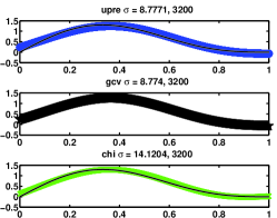
(a) $p=0$ $3200$

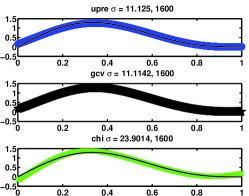
(b) $p=0$ $1600$

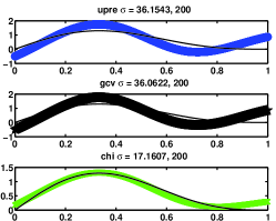
(c) $p=0$ $200$

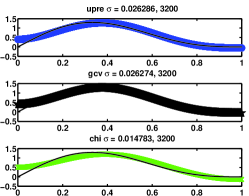
(d) $p=1$ $3200$

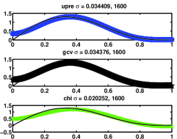
(e) $p=1$ $1600$

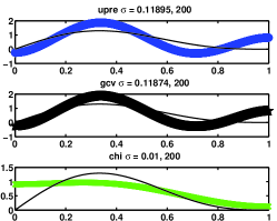
(f) $p=1$ $200$

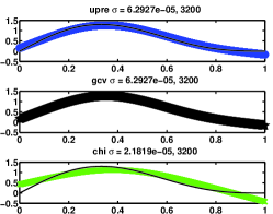
(g) $p=2$ $3200$

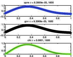
(h) $p=2$ $1600$

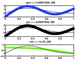
(i) $p=2$ $200$

Figure 1: Illustrative Results for noise level $.1$ for randomly selected sample right hand side in each case, but the same right hand side for each method. The exact solutions are given by the thin lines in each plot.

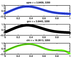
(a) $p=0$ $3200$

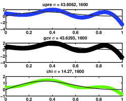
(b) $p=0$ $1600$

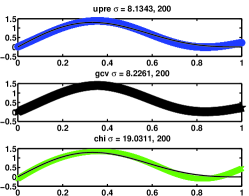
(c) $p=0$ $200$

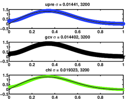
(d) $p=1$ $3200$

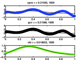
(e) $p=1$ $1600$

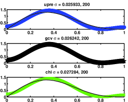
(f) $p=1$ $200$

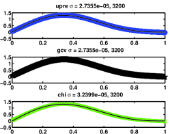
(g) $p=2$ $3200$

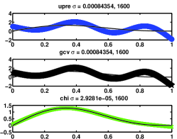
(h) $p=2$ $1600$

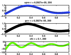
(i) $p=2$ $200$

Figure 2: Illustrative Results for noise level $.01$ for randomly selected sample right hand side in each case, but the same right hand side for each method. The exact solutions are given by the thin lines in each plot.

The quantitative results presented in Tables 1-2, with the best results in each case in bold, demonstrate the remarkable consistency of the UPRE and GCV results. Application of the $\chi^{2}$-principle is not as successful when $L=I$ for which the lack of a useful prior estimate for $\hat{\mathbf{m}}$, theoretically required to apply the central version of Theorem 2.1, has a far greater impact. On the other hand, for derivatives of order $1$ and $2$ this information is less necessary and competitive results are obtained, particularly for the lower noise level. Results in Figures 1-2 demonstrate that all algorithms can succeed, even with significant under sampling, $m=200$, but also may fail even for $m=1600$. When calculating for individual cases, rather than multiple cases at a time as with the results here, it is possible to adjust the number of points used in the minimization for the UPRE or GCV functionals. For the $\chi^{2}$ method it is possible to adjust the tolerance on root finding, or apply filtering of the singular values, with commensurate adjustment of the degrees of freedom, dependent on analysis of the root finding curve. It is clear that these are worst case results for the $\chi^{2}$-principle because of the lack of use of prior information.

$m$	$3200$	$1600$	$800$	$400$	$200$
Method	Derivative Order $0$
UPRE	.175(.088)	.218(.158)	.213(.082)	.239(.098)	$.331(.204)$
GCV	.175(.088)	.218(.158)	.213(.082)	.239(.098)	$.332(.205)$
$\chi^{2}$	$.223(.179)$	$.273(.234)$	$.331(.180)$	$.327(.186)$	.290(.161)
	Derivative Order $1$
UPRE	$.202(.084)$	.248(.151)	.238(.077)	.260(.088)	$.336(.201)$
GCV	$.202(.084)$	.248(.151)	.238(.077)	.260(.088)	$.337(.202)$
$\chi^{2}$	.190(.052)	$.260(.171)$	$.272(.093)$	$.286(.116)$	.305(.065)
	Derivative Order $2$
UPRE	.195(.111)	.246(.160)	.257(.087)	$.280(.094)$	.361(.188)
GCV	.195(.111)	.246(.160)	.257(.087)	.279(.093)	.361(.188)
$\chi^{2}$	$.226(.087)$	$.258(.084)$	$.430(.230)$	$.338(.161)$	$.397(.175)$

Table 1: The mean and standard deviation of the relative error over $25$ copies of the data with noise level $.1$. In each case $n=3200$ and downsampling is obtained by sampling at a sampling rate $1$, $2$, $4$, $8$ and $16$. Best results for each case in boldface.

$m$	$3200$	$1600$	$800$	$400$	$200$
Method	Derivative Order $0$
UPRE	.149(.205)	.075(.122)	.199(.301)	.120(.103)	.139(.081)
GCV	.149(.205)	$.075(.123)$	.199(.301)	$.120(.104)$	.139(.081)
$\chi^{2}$	$.255(.165)$	$.166(.130)$	$.300(.272)$	$.232(.120)$	$.267(.176)$
	Derivative Order $1$
UPRE	$.164(.197)$	$.108(.123)$	$.187(.258)$	$.164(.161)$	.155(.067)
GCV	$.164(.197)$	$.108(.123)$	$.187(.258)$	$.164(.161)$	.155(.067)
$\chi^{2}$	.151(.202)	.088(.030)	.137(.140)	.119(.058)	$.178(.197)$
	Derivative Order $2$
UPRE	$.125(.203)$	$.063(.122)$	$.104(.199)$	$.102(.110)$	.101(.063)
GCV	$.125(.203)$	$.063(.122)$	$.104(.199)$	.095(.103)	.101(.063)
$\chi^{2}$	.051(.034)	.045(.030)	.061(.040)	$.148(.209)$	$.187(.228)$

Table 2: The mean and standard deviation of the relative error over $25$ copies of the data with noise level $.01$. In each case $n=3200$ and downsampling is obtained by sampling at a sampling rate $1$, $2$, $4$, $8$ and $16$. Best results for each case in boldface.

2.4.2 Problem tomo

Figure 3 illustrates results for data contaminated by random noise with variance $.0004$ and $.0001$, $\eta=.02$ and $\eta=.01$, respectively, with solutions obtained with regularization using a first order derivative operator, and sampled using $100\%$, $75\%$ and $50\%$ of the data. At these noise levels, the quality of the solutions when obtained with $m=n$ are also not ideal, but do demonstrate that with reduction of sampling it is still possible to apply parameter estimation techniques to find effective solutions, i.e. all methods succeed in finding useful regularization parameters, demonstrating again that these techniques can be used for under sampled data sets.

Overall the results for gravity and tomo demonstrate that algorithms for regularization parameter estimation can be successfully applied for problems with fewer samples than desirable.

(a) $3600(.301)$

(b) $2700(.329)$

(c) $1800(.387)$

(d) $3600(.224)$

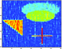
(e) $2700(.268)$

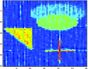
(f) $1800(.332)$

(g) $3600(.302)$

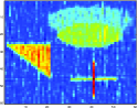
(h) $2700(.328)$

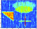
(i) $1800(.380)$

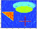
(j) $3600(.230)$

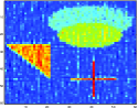
(k) $2700(.278)$

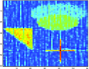
(l) $1800(.384)$

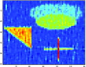
(m) $3600(.297)$

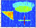
(n) $2700(.325)$

(o) $1800(.380)$

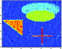
(p) $3600(.222)$

(q) $2700(.263)$

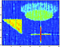
(r) $1800(.325)$

Figure 3: Illustrative results in row $1$ for the UPRE, in row $2$ for the GCV and in row $3$ for the $\chi^{2}$ principle. From left to right problem size $3600$, $2700$ and $1800$, for noise level $.02$ and then $.01$. The label gives the the sample and the relative error $m($error).

3 Algorithmic Considerations for the Iterative MS stabilizer

The results of Section 2.4 demonstrate the relative success of regularization parameter estimation techniques, while also showing that in general with limited data sets improvements may be desirable. Here the iterative technique using the MS stabilizing operator which is frequently used for geophysical data inversion is considered. Its connection with the iteratively regularized norm algorithms, discussed in [32], has apparently not been previously noted in the literature but does demonstrate the convergence of the iteration based on the updating MS stabilizing operator $L$:

$$L^{(k)} =(\mathrm{diag}((\mathbf{m}^{(k-1)}-\mathbf{m}_{\mathrm{0}})^{2})+\epsilon^{2}I)^{-1/2}.$$ (28)

Note $L^{(k)}$ is of size $n\times n$ for all $k$, and the use of small $\epsilon^{2}>0$ assures rank($L^{(k)})=n$, avoiding instability for the components converging to zero, $\mathbf{m}_{j}-(\mathbf{m}_{\mathrm{0}})_{j}\rightarrow 0$. With this $L$ we see that $L=L(\mathbf{m})$ and hence, in the notation of [33] (3) is of pseudo-quadratic form and the iterative process is required. The iteration to find $\mathbf{m}^{(k)}$ from $\mathbf{m}^{(k-1)}$, as in [33], replacing $L$ by $L^{(k)}:=L(\mathbf{m}^{(k-1)})$ transforms (3) to a standard Tikhonov regularization, equivalent to the IRN of [32], which can be initialized with $\mathbf{m}^{(0)}=0$. Theorem 2.1 can be used with $m$ degrees of freedom.

The regularization parameter needed at each iteration can be found by applying any of the noted algorithms, e.g. UPRE, GCV, $\chi^{2}$, MDP, LC-curve, at the $k^{\mathrm{th}}$ iteration, using the SVD calculated for the matrix $\tilde{G}(L^{(k)})^{-1}$, here noting that solving the mapped right preconditioned system is equivalent to solving the original formulation, and avoids the GSVD. In particular (1) in the MS approach is replaced by

$$P^{\sigma_{\mathrm{L}}}(\mathbf{m})=\|G\mathbf{m}-\mathbf{d}_{\mathrm{obs}}\|_{C_{\mathbf{d}}^{-1}}^{2}+(\alpha^{(k)})^{2}\|L^{(k)}(\mathbf{m}-\mathbf{m}^{(k-1)})\|,$$ (29)

with $L^{(k)}$ given by (28), and $\{\alpha^{(k)}\}$ found automatically. In our experiments for the $2D$ gravity model, we contrast the use of an initial zero estimate of the density with an initial estimate for $\mathbf{m}_{0}$ obtained from the data and based on the generalized singular values for which the central form of the $\chi^{2}$ iteration is better justified. For the case with prior information, the initial choice for $\alpha^{(1)}$ is picked without consideration of regularization parameter estimation, and the measures for convergence are for the iterated solutions $\mathbf{m}^{(k)}$, $k\geq 1$.

3.1 Numerical Results: A $2D$ Gravity Model

We contrasted the use of the regularization parameter estimations techniques on an underdetermined $2D$ gravity model. Figure 4(a)-4(b) shows this model and its gravity value.

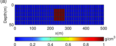
(a) Original Model

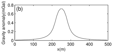
(b) Gravity Anomaly

Figure 4: (a) Model of a body set in a grid of square cells each of size $10$m, the density contrast of the body is $1\mathrm{gr}/\mathrm{cm}^{3}$. (b) The gravity anomaly due to the synthetic model.

The synthetic model is a rectangular body, $60\mathrm{m}\times 30\mathrm{m}$, that has density contrast $1\mathrm{gr}/\mathrm{cm}^{3}$ with an homogeneous background. Simulation data are calculated at $50$ stations with $10\mathrm{m}$ spacing on the surface. The subsurface is divided into $50\times 5$ cells with $10\mathrm{m}\times 10\mathrm{m}$ dimension, hence in this case $m=50$ and $n=250$. In generating noise-contaminated data we generate a random matrix $\Theta$ of size $m\times 50$, with columns $\Theta^{c}$, $c=1:50$, using the MATLAB function $\bf{randn}$. Then setting $\mathbf{d}^{c}=\mathbf{d}+\left(\eta_{1}\left(\mathbf{d}_{\mathrm{exact}}\right)_{i}+\eta_{2}\|\mathbf{d}_{\mathrm{exact}}\|\right)\Theta^{c}$, generates $50$ copies of the right-hand vector $\mathbf{d}$. Results of this $20\%$ under sampling are presented for $3$ noise levels, namely ($\eta_{1}=0.01,\eta_{2}=0.001$;$\eta_{1}=0.03,\eta_{2}=0.005$ and $\eta_{1}=0.05,\eta_{2}=0.01$).

In the experiments we contrast not only the GCV, UPRE and $\chi^{2}$ methods, but also the MDP and L-curve which are the standard techniques in the related geophysics literature. Details are as follows:

Depth Weighting Matrix

Potential field inversion requires the inclusion of a depth weighting matrix within the regularization term. We use $\beta=0.6$ in the diagonal matrix $(W_{\mathrm{depth}})_{jj}=z_{j}^{-\beta}$ for cell $j$ at depth $z_{j}$, and at each step form the column scaling through $\tilde{G}^{(k)}=\tilde{G}(W_{\mathrm{depth}})^{-1}(L^{(k)})^{-1}$, where in $L^{(k)}$ $\epsilon=.02$.

Initialization

In all cases the inversion is initialized with a $\mathbf{m}^{(0)}=\mathbf{m}_{0}$ which is obtained as the solution of the regularized problem, with depth weighting, and found for the fixed choice $\alpha^{(0)}=(n/m)\max(\gamma_{i})/\mathrm{mean}(\gamma_{i})$, using the singular values of the weighted $\tilde{G}$. All subsequent iterations calculate $\alpha^{(k)}$ using the chosen regularization parameter estimation technique.

Stopping Criteria

The algorithm terminates for $k=k_{\mathrm{final}}$ when one of the following conditions is met, with $\tau=.01$,

(i) a sufficient decrease in the functional is observed, $P^{\alpha^{(k-1)}}-P^{\alpha^{(k)}}<\tau(1+P^{\alpha^{(k)}})$,

(ii) the change in the density satisfies $\|\mathbf{m}^{(k-1)}-\mathbf{m}^{(k)}\|<\sqrt{\tau}(1+\|\mathbf{m}^{(k)}\|)$,

(iii) a maximum number of iterations, $K$, is reached, here $K=20$.

Bound Constraints

Based on practical knowledge the density is constrained to lie between $[0,1]$ and any values outside the interval are projected to the closest bound.

$\chi^{2}$ algorithm

The Newton algorithm used for the $\chi^{2}$ algorithm is iterated to tolerance determined by a confidence interval $\theta=.95$ in (27), dependent on the number of degrees of freedom, corresponding to $0.6271$ for $50$ degrees of freedom. The maximum degrees of freedom is adjusted dynamically dependent on the number of significant singular values, with the tolerance adjusted at the same time. We note that the number of degrees of freedom often drops with the iteration and thus the tolerance increases, but that the difference in results with choosing lower tolerance $\theta=.90$, leads to almost negligible change in the results.

Exploring $\alpha$

At each step for the L-curve, MDP, GCV and UPRE, the solution is found at each iteration for $1000$ choices of $\alpha$ over a range dictated by the current singular values, see the discussion for the L-cuve in e.g. [1, 9].

MDP algorithm

To find $\alpha$ by the MDP we interpolate $\alpha$ against the weighted residual for $1000$ values for $\alpha$ and use the Matlab function interp1 to find the $\alpha$ which solves for the degrees of freedom. Here we use $\delta=m$ so as to avoid the complication in the comparison of how to scale $M$, i.e. we use $\rho=1$.

Tables 3-5 contrast the performance of the $\chi^{2}$ discrepancy, MDP, LC, GCV and UPRE methods with respect to relative error, ${\|\left(\mathbf{m}_{\mathrm{exact}}-\mathbf{m}^{(K)}\right)\|_{2}}/{\|\mathbf{m}_{\mathrm{exact}}\|_{2}}$, and the average regularization parameter calculated at the final iteration. We also record the average number of iterations required to convergence. In Table 3 we also give the relative errors after one just one iteration of the MS and with the zero initial condition.

Table 3: Mean and standard deviation of the relative error measured in the $2-$norm with respect to the known solution over 50 runs. Again the best results in each case are indicated by the boldface entries.

	Method
Noise	UPRE	GCV	$\chi^{2}$	MDP	LC
$\eta_{1},\eta_{2}$	Results after just one step, non zero initial condition
$0.01,0.001$	$.331(.008)$	.325(.008)	.325(.008)	$.355(.009)$	$.447(.055)$
$0.03,0.005$	.353(.019)	$.354(.042)$	$.361(.020)$	$.418(.025)$	$.374(.052)$
$0.05,0.01$	.392(.034)	$.409(.062)$	$.416(.040)$	$.478(.043)$	$.463(.067)$
	Results using the non zero initial condition
$0.01,0.001$	$.323(.009)$	$.314(.010)$	.317(.009)	$.352(.011)$	$.489(.078)$
$0.03,0.005$	.339(.022)	$.338(.040)$	$.359(.022)$	$.413(.026)$	$.369(.053)$
$0.05,0.01$	.374(.041)	$.393(.068)$	$.414(.041)$	$.470(.046)$	$.460(.070)$
	Results using the initial condition $\mathbf{m}_{0}=0$
$0.01,0.001$	$.322(.001)$	$.312(.011)$	.315(.001)	$.359(.009)$	$.593(.014)$
$0.03,0.005$	.333(.020)	$.334(.037)$	$.352(.021)$	$.425(.026)$	$.451(.067)$
$0.05,0.01$	.357(.030)	$.440(.086)$	$.388(.034)$	$.477(.046)$	$.487(.082)$

Table 4: Mean and standard deviation of $\alpha^{k_{\mathrm{final}}}$ over $50$ runs.

Noise	Method
$\eta_{1},\eta_{2}$	UPRE	GCV	$\chi^{2}$	MDP	LC
$0.01,0.001$	$35.49(5.17)$	$14.93(9.85)$	$91.32(30.56)$	$53.42(7.43)\,\,$	$3.83(1.91)$
$0.03,0.005$	$11.02(2.62)$	$\,\,4.18(2.58)$	$72.71(32.72)$	$30.90(8.21)\,\,$	$0.86(0.08)$
$0.05,0.01$	$\,\,7.64(4.35)$	$\,\,3.28(3.05)$	$89.79(27.97)$	$25.81(14.87)$	$0.46(0.05)$

Table 5: Mean and standard deviation of the number of iterations $k_{\mathrm{final}}$ to meet the convergence criteria over $50$ runs. Again the best results in each case are indicated by the boldface entries.

Noise	Method
$\eta_{1},\eta_{2}$	UPRE	GCV	$\chi^{2}$	MDP	LC
$0.01,0.001$	$18.94(0.31)$	$14.78(5.83)$	$16.26(3.00)$	$18.32(1.10)$	6.30(1.64)
$0.03,0.005$	$11.90(2.76)$	$\,\,9.22(2.86)$	5.50(1.39)	$\,\,7.68(1.80)$	$7.90(2.48)$
$0.05,0.01$	$\,\,7.82(1.73)$	$\,\,8.22(2.41)$	5.10(0.58)	$\,\,5.72(0.97)$	$7.84(2.41)$

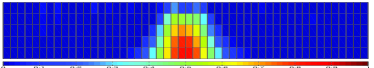
(a) Initial Gravity

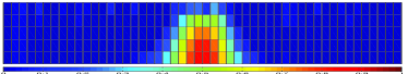
(b) Initial Gravity

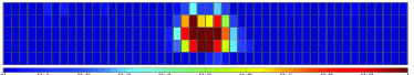
(c) UPRE: error $.3181$

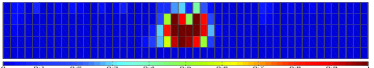
(d) UPRE: error $.3122$

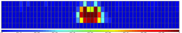
(e) GCV: error $.3196$

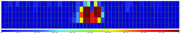
(f) GCV: error $.3747$

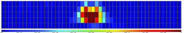
(g) $\chi^{2}$: error $.3381$

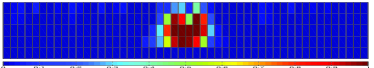
(h) $\chi^{2}$: error $.3154$

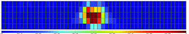
(i) MDP: error $.3351$

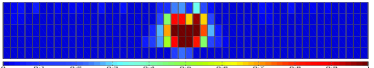
(j) MDP: error $.3930$

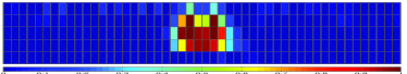
(k) LC: error $.3328$

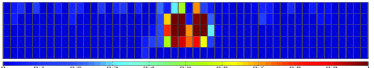
(l) LC: error $.4032$

Figure 5: Density model obtained from inverting the noise-contaminated data. The regularization parameter was found using the UPRE in 7(a)-7(b), the GCV in 7(c)-7(d), the $\chi^{2}$ in 7(e)-7(f), the MDP in 7(g)-7(h), and the L-Curve in 7(i)-7(j). In each case the initial value $\mathbf{m}_{0}^{(0)}$ is illustrated in 5(a)-5(b), respectively. The data are two cases with noise level, $\eta_{1}=.03$ and $\eta_{2}=.005$, with on the left a typical result, sample $37$ and and on the right one of the few cases of $50$ with sometimes larger error, sample $22$. One can see that results are overall either consistently good or consistently poor, except that the $\chi^{2}$ and UPRE results are not bad in either case.

With respect to the relative error one can see that the error increases with the noise level, except that the L-curve appears to solve the second noise level situation with more accuracy. In most regards the UPRE, GCV and $\chi^{2}$ methods behavior similarly, with relative stability of the error (smaller standard deviation in the error), and increasing error with noise level. On the other hand, the final value of the regularization parameter is not a good indicator of whether a solution is over or under smoothed, contrast e.g. the $\chi^{2}$ and GCV methods. The $\chi^{2}$ method is overall cheaper, fewer iterations are required and the cost per iteration is cheap, not relying on an exploration with respect to $\alpha$, interpolation or function minimization. The illustrated results in Figure 5, for the second noise level, $\eta_{1}=.03$ and $\eta_{2}=.005$, for a typical result, sample $37$ and one of the few cases from $50$ with larger error, sample $22$, demonstrate that all methods achieve some degree of acceptable solution with respect to moving from an initial estimate which is inadequate to a more refined solution. In all cases the geometry and density of the reconstructed models are close to those of the original model.

To demonstrate that the choice of the initial $\mathbf{m}_{0}$ is useful for all methods, and not only the $\chi^{2}$ method we show the same results as in Figure 5 but initialized with $\mathbf{m}_{0}=0$. In most cases the solutions that are obtained are less stable, indicating that the initial estimate is useful in constraining the results to reasonable values, however most noticeably not for the $\chi^{2}$ method, but for the MDP and L-curve algorithms. We also illustrate the results obtained after just one iteration in Figure 7 with the initial condition $\mathbf{m}_{0}$ according to Figure 5 to demonstrate the need for the iteration to generally stabilize the results. These results confirm the relative errors shown in Table 3 for averages of the errors over the $50$ cases.

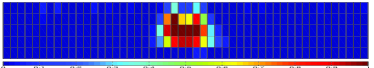
(a) UPRE: error $.3174$

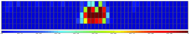
(b) UPRE: error $.3240$

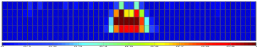
(c) GCV: error $.3162$

(d) GCV: error $.3718$

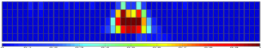
(e) $\chi^{2}$: error $.3356$

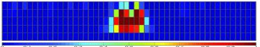
(f) $\chi^{2}$: error $.3314$

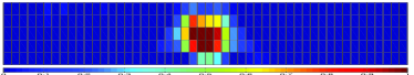
(g) MDP: error $.4042$

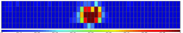
(h) MDP: error $.3356$

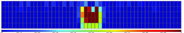
(i) LC: error $.4420$

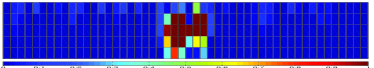
(j) LC: error $.4555$

Figure 6: Density model obtained from inverting the noise-contaminated data, as in Figure 5 except initialized with $\mathbf{m}_{0}=0$

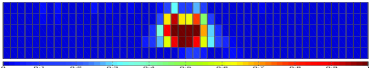
(a) UPRE: error $.3330$

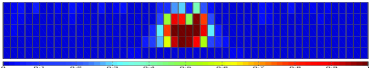
(b) UPRE: error $.3214$

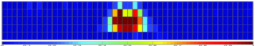
(c) GCV: error $.3316$

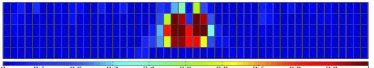
(d) GCV: error $.3693$

(e) $\chi^{2}$: error $.3398$

(f) $\chi^{2}$: error $.3217$

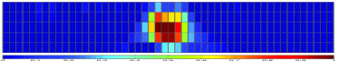
(g) MDP: error $.4006$

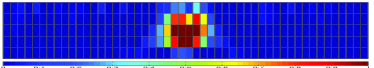
(h) MDP: error $.3458$

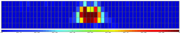
(i) LC: error $.3299$

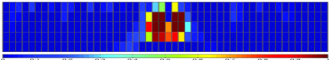
(j) LC: error $.3970$

Figure 7: Density model obtained from inverting the noise-contaminated data, as in Figure 5 after just one step of the MS iteration.

4 Conclusions

The UPRE, GCV and $\chi^{2}$-principle algorithms for estimating a regularization parameter in the context of underdetermined Tikhonov regularization have been developed and investigated, extending the $\chi^{2}$ method discussed in [13, 14, 15, 16, 17]. UPRE and $\chi^{2}$ techniques require that an estimate of the noise distribution in the data measurements is available, while ideally the $\chi^{2}$ also requires a prior estimate of the mean of the solution in order to apply the central version of the $\chi^{2}$ algorithm. Results demonstrate that UPRE, GCV and $\chi^{2}$ techniques are useful for under sampled data sets, with UPRE and GCV yielding very consistent results. The $\chi^{2}$ is more useful in the context of the mapped problem where prior information is not required. On the other hand, we have shown that the use of the iterative MS stabilizer provides an effective alternative to the non-central algorithm suggested in [17] for the case without prior information. The UPRE, GCV and $\chi^{2}$ generally outperform L-curve and MDP methods to find the regularization parameter in the context of the iterative MS stabilizer for $2D$ gravity inversion. Moreover, with regard to efficiency the $\chi^{2}$ generally requires fewer iterations, and is also cheaper to implement for each iteration because there is no need to sweep through a large set of $\alpha$ values in order to find the optimal value. These results are useful for the development of approaches for solving larger $3D$ problems of gravity inversion, which will be investigated in future work. Then, the ideas have to be extended for iterative techniques replacing the SVD or GSVD for the solution.

Appendix 0.A Parameter Estimation Formulae

We assume that the matrices and data are pre weighted by the covariance of the data, and thus use the GSVD of Lemma 1 for the matrix pair $[\tilde{G};L]$. We also introduce inclusive notation for the limits of the summations, that are correct for all choices of $(m,n,p,r)$, where $r\leq\min(m,n)$ determines filtering of the least $p-r-\tilde{q}$ singular values $\gamma_{i}$, $\tilde{q}=\max(n-m,0)$. Then $\mathbf{m}(\sigma_{\mathrm{L}})=\mathbf{m}_{\mathrm{0}}+\mathbf{y}(\sigma_{\mathrm{L}})$ is obtained for

$$\mathbf{y}(\sigma_{\mathrm{L}}) =\sum_{i=\tilde{q}+1}^{p}\frac{\nu_{i}}{\nu_{i}^{2}+\sigma_{\mathrm{L}}^{-2}\mu_{i}^{2}}s_{i}\mathbf{z}_{i}+\sum_{i=p+1}^{n}s_{i}\mathbf{z}_{i}=\sum_{i=q+1}^{p}f_{i}\frac{s_{i}}{\nu_{i}}\mathbf{z}_{i}+\sum_{i=p+1}^{n}s_{i}\mathbf{z}_{i},$$ (30)

where $Z:=(X^{T})^{-1}=[\mathbf{z}_{1},\dots,\mathbf{z}_{n}]$, ,$f_{i}=\left(\frac{\gamma_{i}^{2}}{\gamma_{i}^{2}+\sigma_{\mathrm{L}}^{-2}}\right)$ are the filter factors and $s_{i}=\mathbf{u}_{i-\tilde{q}}^{T}\tilde{\mathbf{r}}$, $s_{i}=0$, $i<q$. Orthogonal matrix $V$ replaces $(X^{T})^{-1}$ and $\sigma_{i}$ replaces $\gamma_{i}$, when applied for the singular value decomposition $\tilde{G}=U\Sigma V^{T}$ with $L=I$.

Let $\tilde{s}_{i}(\sigma_{\mathrm{L}})={s_{i}}/{(\gamma_{i}^{2}\sigma_{\mathrm{L}}^{2}+1)}$, and note the filter factors with truncation are given by

$$f_{i}=\left\{\begin{array}[]{ll}0&\tilde{q}+1\leq i\leq p-r\\ \frac{\gamma_{i}^{2}}{\gamma_{i}^{2}+\sigma_{\mathrm{L}}^{-2}}&p-r+1\leq i\leq p\\ 1&p+1\leq n\end{array}\right.\quad(1-f_{i})=\left\{\begin{array}[]{ll}1&\tilde{q}+1\leq i\leq p-r\\ \frac{1}{\gamma_{i}^{2}\sigma_{\mathrm{L}}^{2}+1}&p-r+1\leq i\leq p\\ 0&p+1\leq n\end{array}\right..$$ (37)

Then, with the assumption that if a lower limit is lower than a higher limit on a sum the contribution is $0$,

$$\mathrm{trace}(I_{m}-G(\sigma_{\mathrm{L}})) =m-\sum_{i=\tilde{q}+1}^{\min(n,m)}f_{i}=(m-(n-(p-r)))+\sum_{i=p-r+1}^{\min(n,m)}(1-f_{i})$$

$$=(m+p-n-r)+\sum_{i=p-r+1}^{p}\frac{1}{\gamma_{i}^{2}\sigma_{\mathrm{L}}^{2}+1}:=T(\sigma_{\mathrm{L}})$$ (38)

$$\|(I_{m}-G(\sigma_{\mathrm{L}}))\tilde{\mathbf{r}}\|_{2}^{2} =\sum_{i=p-r+1}^{p}(1-f_{i})^{2}s_{i}^{2}+\sum_{i=n+1}^{m}s_{i}^{2}+\sum_{i=\tilde{q}+1}^{p-r}s_{i}^{2}$$ (39)

$$=\sum_{i=p-r+1}^{p}\tilde{s}_{i}^{2}(\sigma_{\mathrm{L}})+\sum_{i=n+1}^{m}s_{i}^{2}+\sum_{i=\tilde{q}+1}^{p-r}s_{i}^{2}:=N(\sigma_{\mathrm{L}}).$$ (40)

Therefore we seek in each case $\sigma_{\mathrm{L}}$ as the root, minimum or corner of a given function.

UPRE:

Minimizing $(\|\tilde{G}\mathbf{y}(\sigma_{\mathrm{L}})-\tilde{\mathbf{r}}\|_{2}^{2}+2\,\mathrm{trace}(G(\sigma_{\mathrm{L}}))-m)$ we may shift by constant terms and minimize

$$U(\sigma_{\mathrm{L}}) =\sum_{i=p-r+1}^{p}(1-f_{i})^{2}s_{i}^{2}+2\sum_{i=p-r+1}^{p}(f_{i}-1)=\sum_{i=p-r+1}^{p}\tilde{s}_{i}^{2}-2\sum_{i=p-r+1}^{p}\frac{1}{\gamma_{i}^{2}\sigma_{\mathrm{L}}^{2}+1}.$$ (41)

GCV:

Minimize

$$GCV(\sigma_{\mathrm{L}}) =\frac{\|\tilde{G}\mathbf{y}(\sigma_{\mathrm{L}})-\tilde{\mathbf{r}}\|_{2}^{2}}{\mathrm{trace}(I_{m}-G(\sigma_{\mathrm{L}}))^{2}}=\frac{N(\sigma_{\mathrm{L}})}{T^{2}(\sigma_{\mathrm{L}})}$$ (42)

$\chi^{2}$-principle

The iteration to find $\sigma_{\mathrm{L}}$ requires

$$\|\mathbf{k}(\sigma_{\mathrm{L}})\|_{2}^{2} =\sum_{i=q+1}^{p}\frac{s_{i}^{2}}{\gamma_{i}^{2}\sigma_{\mathrm{L}}^{2}+1},\,\frac{\partial{\|\mathbf{k}(\sigma_{\mathrm{L}})\|_{2}^{2}}}{\partial\sigma_{\mathrm{L}}}=-2\sigma_{\mathrm{L}}\sum_{i=q+1}^{p}\frac{\gamma_{i}^{2}s_{i}^{2}}{(\gamma_{i}^{2}\sigma_{\mathrm{L}}^{2}+1)^{2}}=-\frac{2}{\sigma_{\mathrm{L}}^{3}}\|L\mathbf{y}(\sigma_{\mathrm{L}})\|_{2}^{2},$$ (43)

and with a search parameter $\beta^{(j)}$ uses the Newton iteration

$$\sigma^{(j+1)}=\sigma^{(j)}\left(1+\beta^{(j)}\frac{1}{2}\left(\frac{\sigma^{(j)}}{\|L\mathbf{y}(\sigma^{(j)})\|_{2}}\right)^{2}(\|\mathbf{k}(\sigma^{(j)})\|_{2}^{2}-(m+p-n))\right).$$ (44)

This iteration holds for the filtered case by defining $\gamma_{i}=0$ for $q+1\leq i\leq p-r$, removing the constant terms in (26) and using $r$ degrees of freedom, [22].

MDP

: For $0<\rho\leq 1$ and $\delta=m$, solve

$$\|(I_{m}-G(\sigma_{\mathrm{L}}))\tilde{\mathbf{r}}\|_{2}^{2}=N(\sigma_{\mathrm{L}})=\rho\delta.$$ (45)

L-curve:

Determine the corner of the log-log plot of $\|L\mathbf{y}\|_{2}$ against $\|\tilde{G}\mathbf{y}(\sigma_{\mathrm{L}})-\tilde{\mathbf{r}}\|_{2}$, namely the corner of the curve parameterized by

$$\left(\sqrt{N(\sigma_{\mathrm{L}})},\sigma_{\mathrm{L}}^{2}\sqrt{\sum_{i=p-r+1}^{p}\frac{\gamma_{i}^{2}s_{i}^{2}}{(\gamma_{i}^{2}\sigma_{\mathrm{L}}^{2}+1)^{2}}}\right).$$

References

References

- [1] Aster R C, Borchers B and Thurber C H 2013 Parameter Estimation and Inverse Problems second edition Elsevier Inc. Amsterdam.
- [2] Donatelli M, Hanke M 2013 Fast nonstationary preconditioned iterative methods for ill-posed problems, with application to image deblurring Inverse Problems 29 9 095008.
- [3] Engl H W, Hanke M and Neubauer A 1996 Regularization of Inverse Problems Kluwer Dordrecht.
- [4] Golub G H, Heath M and Wahba G 1979 Generalized Cross Validation as a method for choosing a good ridge parameter Technometrics 21 2 215-223.
- [5] Golub G H and van Loan C 1996 Matrix Computations (John Hopkins Press Baltimore) 3rd ed.
- [6] Hanke M and Groetsch CW 1998 Nonstationary iterated Tikhonov regularization J. Optim. Theor. Appl. 98 37-53.
- [7] Hansen P C 1992 Analysis of discrete ill-posed problems by means of the L-curve SIAM Review 34 561-580.
- [8] Hansen P C 1998 Rank-Deficient and Discrete Ill-Posed Problems: Numerical Aspects of Linear Inversion SIAM Monographs on Mathematical Modeling and Computation 4 Philadelphia.
- [9] Hansen, P. C., 2007, Regularization Tools Version 4.0 for Matlab 7.3, Numerical Algorithms, 46, 189-194, and http://www2.imm.dtu.dk/~pcha/Regutools/.
- [10] Hansen P C, Kilmer M E and Kjeldsen R H 2006 Exploiting residual information in the parameter choice for discrete ill-posed problems BIT 46 41-59.
- [11] Li Y and Oldenburg D W 1999 3D Inversion of DC resistivity data using an L-curve criterion 69th Ann. Internat. Mtg., Soc. Expl. Geophys. Expanded Abstracts 251-254.
- [12] Marquardt D W 1970 Generalized inverses, ridge regression, biased linear estimation, and nonlinear estimation Technometrics 12 (3) 591-612.
- [13] Mead J L 2008 Parameter estimation: A new approach to weighting a priori information Journal of Inverse and Ill-Posed Problems 16 2 175-194.
- [14] Mead J L 2013 Discontinuous parameter estimates with least squares estimators Applied Mathematics and Computation 219 5210-5223.
- [15] Mead J L and Hammerquist C C 2013 tests for choice of regularization parameter in nonlinear inverse problems SIAM Journal on Matrix Analysis and Applications 34 3 1213-1230.
- [16] Mead J L and Renaut R A 2009 A Newton root-finding algorithm for estimating the regularization parameter for solving ill-conditioned least squares problems Inverse Problems 25 025002 doi: 10.1088/0266-5611/25/2/025002.
- [17] Mead J L and Renaut R A 2010 Least Squares problems with inequality constraints as quadratic constraints Linear Algebra and its Applications 432 8 1936-1949 doi:10.1016/j.laa.2009.04.017.
- [18] Morozov V A 1966 On the solution of functional equations by the method of regularization Sov. Math. Dokl. 7 414-417.
- [19] Paige C C and Saunders M A 1981 Towards a generalized singular value decomposition SIAM Journal on Numerical Analysis 18 3 398-405.
- [20] Paige C C and Saunders M A 1982 LSQR: An algorithm for sparse linear equations and sparse least squares ACM Trans. Math. Software 8 43-71.
- [21] Paige C C and Saunders M A 1982 ALGORITHM 583 LSQR: Sparse linear equations and least squares problems ACM Trans. Math. Software 8 195-209.
- [22] Renaut R A, Hnetynková I and Mead J L 2010 Regularization parameter estimation for large scale Tikhonov regularization using a priori information Computational Statistics and Data Analysis 54 12 3430-3445 doi:10.1016/j.csda.2009.05.026.
- [23] Ring W 1999 Structural Properties of solutions of Total Variation regularization problems Preprint http://www.uni-graz.at/imawww/ring/publist.html
- [24] Rudin L I Osher S and Fatemi E 1992 Nonlinear total variation based noise removal algorithms, Physica D 60 259-268.
- [25] Portniaguine O and Zhdanov M S 1999 Focusing geophysical inversion images Geophysics 64 874-887.
- [26] Rust B W and O’Leary D.P 2008 Residual periodograms for choosing regularization parameters for ill-posed problems Inverse Problems 24 034005.
- [27] Stefan W Garnero E and Renaut R A 2006 Signal restoration through deconvolution applied to deep mantle seismic probes Geophysical Journal International 167 1353-1362.
- [28] Tarantola A 2005 Inverse Problem Theory and Methods for Model Parameter Estimation SIAM Series: Other Titles in Applied Mathematics Philadelphia U.S.A.
- [29] Thompson A M, Kay J W and Titterington D M 1991 Noise Estimation in Signal Restoration using Regularization Biometrika 78 3 475-488.
- [30] Vatankhah S Ardestani V E and Renaut R A 2013 Automatic estimation of the regularization parameter in 2-D focusing gravity inversion: an application to the Safo manganese mine in northwest of Iran, to appear, J Geophysics and Engineering http://arxiv.org/abs/0813162
- [31] Vogel C R 2002 Computational Methods for Inverse Problems SIAM Frontiers in Applied Mathematics SIAM Philadelphia U.S.A.
- [32] Wohlberg B and Rodriguez P 2007 An Iteratively Reweighted Norm Algorithm for Minimization of Total Variation Functionals IEEE Signal Processing Letters 14 948–951.
- [33] Zhdanov M S 2002 Geophysical Inverse Theory and Regularization Problems Elsevier Amsterdam.