Constraining axion-nucleon coupling constants from measurements of effective Casimir pressure by means of micromachined oscillator

Abstract

Stronger constraints on the pseudoscalar coupling constants of an axion to a proton and a neutron are obtained from an indirect measurement of the effective Casimir pressure between two Au-coated plates by means of micromechanical torsional oscillator. For this purpose, the additional effective pressure due to two-axion exchange is calculated. The role of boundary effects and the validity region of the proximity force approximation in application to forces of axion origin are determined. The obtained constraints are up to factors of 380 and 3.2 stronger than those found recently from other laboratory experiments and are relevant to axion masses from $10^{-3}\,$eV to 15 eV.

1 Introduction

Starting from the prediction of axions in 1978 1 ; 2 , axion physics has become a wide subject stimulating development of elementary particle theory, gravitation and cosmology (see 3 ; 4 for a review). Axions are pseudoscalar particles which appear as a consequence of breaking the Peccei and Quinn symmetry 5 . They provide an elegant solution for the problem of strong CP violation and large electric dipole moment for the neutron in QCD. Since the proper QCD axions were constrained to a narrow band in parameter space 5a , a lot of invisible axion-like particles have been proposed in different unification schemes. Among others, the models of the hadronic (KSVZ) 6 ; 7 and the GUT (DFSZ) 8 ; 9 axions, which can be used to solve the problem of strong CP violation in QCD, have attracted particular attention (see, for instanse, a number of variants of the model of hadronic axion containing the relationship between the axion-nucleon coupling constant and the Peccei-Quinn symmetry breaking scale 9a ; 9b ). At the moment axion-like particles with masses $m_{a}$ from approximately $10^{-5}\,$eV to $10^{-2}\,$eV and of about 1 MeV are not excluded by astrophysical constraints 4 ; 10 . Keeping in mind that the latter may be more model-dependent than the laboratory constraints 11 ; 12 , it seems warranted to look for some alternative phenomena which could be used for constraining axion-like particles of any mass. Additional interest in this subject is due to the role of axions as possible constituents of dark matter 12a ; 12b .

Previously constraints on axion-nucleon coupling constants have been obtained 13 ; 14 ; 15 from the laboratory experiments of Eötvos 15 ; 16 and Cavendish 17 ; 21a type. At first, this analysis was performed for massless axions but later it was generalized 18 for the case of massive ones. The resulting constraints were found in the range of axion masses from approximately $10^{-9}\,$eV to $10^{-5}\,$eV. In 19 constraints on the axion-nucleon coupling constants were obtained from measurements of the thermal Casimir-Polder force between a Bose-Einstein condensate of ⁸⁷Rb atoms and a SiO₂ plate 48 . These constraints refer to larger axion masses from $10^{-4}\,$eV to 0.3 eV. In fact, the effective potential arising between two fermions from the exchange of a pseudoscalar axion-like particle is spin-dependent 18 . Taking into account that the test bodies in the experiments 15 ; 16 ; 17 ; 21a ; 48 are unpolarized, the aditional force constrained in 18 ; 19 comes from the two-axion exchange.

Using the same approach, in 20 stronger constraints on axion-nucleon coupling constants over the wide range of axion masses from $3\times 10^{-5}\,$eV to 1 eV were obtained from measurements of the Casimir force gradient between a sphere and a plate coated with nonmagnetic and magnetic metals performed by means of dynamic atomic force microscope 21 ; 22 ; 23 ; 24 ; 25 . The strengthening up to a factor of 170, as compared to the constraints of 19 , was achieved. This demonstrates that various experiments on measuring the Casimir interaction 26 are promising for further constraining the parameters of an axion. In the past, these experiments were successfully used to obtain stronger constraints on the Yukawa-type corrections to Newtonian gravity due to exchange of light scalar particles 27 and from extra-dimensional physics with low-energy compactification scale 28 (see review 29 and the most recent results 30 ; 31 ; 32 ; 33 ; 34 ; 35 ).

In this paper, we obtain stronger constraints on the pseudoscalar coupling constants of axion-like particles to a proton and a neutron from measurements of the effective Casimir pressure by means of micromechanical torsional oscillator 36 ; 37 . For this purpose, we calculate the additional effective pressure in the configuration of two parallel plates arising due to two-axion exchange between a sphere and a plate (note that the experimental configuration 36 ; 37 involves a sphere oscillating in the perpendicular direction to the plate, so that the effective pressure arises in the proximity force approximation 26 ; 29 ). The stronger limits on axion-nucleon coupling constants are obtained over the range of axion masses from $10^{-3}\,$eV to 15 eV. The strengthening by factors from 2.2 to 3.2 in comparison with the limits of 20 is achieved over the range of axion masses from $10^{-3}\,$eV to 1 eV, respectively. As compared to the limits of 19 , the obtained constraints are stronger up to a factor of 380. Our model-independent constraints are applicable on equal terms to axions and axion-like particles. Because of this, below both terms are used synonymously. All equations are written in the system of units with $\hbar=c=1$.

2 Pressure between two metallic plates due to two-axion exchange

In the experiment 36 ; 37 , the effective Casimir pressure between two Au plates was determined from dynamic measurements using a micromechanical torsional oscillator. The oscillator consisted of a heavily doped polysilicon plate of area $500\times 500\,\mu\mbox{m}^{2}$ and thickness $D=5\,\mu$m suspended at two opposite points above the platform at the height of about $2\,\mu$m. Two independent electrodes located on the platform under the plate were used to measure the capacitance between the electrodes and the plate. They were also used to induce oscillation in the plate at the resonance frequency of the micromachined oscillator. A large sapphire sphere coated with layers of Cr and Au was attached to the optical fiber above the oscillator. The sphere radius was measured to be $R=151.3\,\mu$m. A silicon plate below the sphere was also coated with layers of Cr and Au.

In the dynamic measurements, the vertical separation between the sphere and the plate was varied harmonically with the resonance frequency of oscillator, $\omega_{r}$, in the presence of the sphere. The Casimir force between the sphere and the plate caused the difference between $\omega_{r}$ and the natural frequency of the oscillator $\omega_{0}$. This difference has been measured and recalculated into the gradient of the Casimir force acting between the sphere and the plate, $F_{sp}^{\prime}(a)$, using the solution for the linear oscillator motion ($a$ is the absolute sphere-plate separation). According to the proximity force approximation (PFA) 26 ; 29 ,

$$F_{sp}(a)=2\pi RE(a),$$ (1)

where $E(a)$ is the Casimir energy per unit area of two parallel plates (semispaces). Calculating the negative derivative of both sides of (1), one obtains the effective Casimir pressure between two parallel plates

$$P(a)=-\frac{1}{2\pi R}F_{sp}^{\prime}(a),$$ (2)

which is the physical quantity indirectly measured in 36 ; 37 . Note that under the condition $a\ll R$ the relative error in the gradient of the Casimir force computed using (1) does not exceed $(0.3-0.4)a/R$ 38 ; 38a ; 39 ; 40 ; 41 . Taking into account that below we consider separations $a<300\,$nm, this is of less than 0.1% error.

Now we calculate the additional pressure between two parallel semispaces separated with a gap $a$ due to two-axion exchange between nucleons. In this section, we consider homogeneous semispaces and postpone the account of finite thickness of the plate and layer structure of both test bodies to Secs. 3 and 4. First we perform a direct derivation of the additional pressure $P_{\rm add}(a)$ by summing up the energies of pair nucleon-nucleon interactions over the two semispaces and calculating the negative derivative of the obtained result. This pressure can be considered as an addition to the indirectly measured Casimir pressure (2) if the additional force between a sphere and a plate due to two-axion exchange is related to the additional energy per unit area of two parallel plates by the PFA, so that

$$F_{sp,{\rm add}}(a)=2\pi RE_{\rm add}(a),$$ (3)

$$P_{\rm add}(a)=-\frac{1}{2\pi R}F_{sp,{\rm add}}^{\prime}(a).$$

Then we determine the application region of (3) from the comparison with the exact result for $F_{sp,{\rm add}}^{\prime}(a)$.

Let the coordinate plane $x,\,y$ coincide with the boundary plane of the lower semispace and let the $z$ axis be perpendicular to it. The effective potential due to two-axion exchange between two nucleons (protons or neutrons) situated at the points $\mbox{\boldmath$r$}_{1}$ and $\mbox{\boldmath$r$}_{2}$ of the upper and lower semispaces, respectively, is given by 18 ; 42 ; 43

$$V_{kl}(|\mbox{\boldmath$r$}_{1}-\mbox{\boldmath$r$}_{2}|)=-\frac{g_{ak}^{2}g_{al}^{2}\,m_{a}}{32\pi^{3}m^{2}}\,\frac{K_{1}(2m_{a}|\mbox{\boldmath$r$}_{1}-\mbox{\boldmath$r$}_{2}|)}{(\mbox{\boldmath$r$}_{1}-\mbox{\boldmath$r$}_{2})^{2}}.$$ (4)

Here, $g_{ak}$ and $g_{al}$ are the coupling constants of an axion to a proton ($k,\,l=p$) or a neutron ($k,\,l=n$) interaction, $m=(m_{n}+m_{p})/2$ is the mean of the neutron and proton masses, and $K_{1}(z)$ is the modified Bessel function of the second kind. Equation (4) was derived under the condition $|\mbox{\boldmath$r$}_{1}-\mbox{\boldmath$r$}_{2}|\gg 1/m$. Taking into acount that in the experiment 36 ; 37 we have $a>160\,$nm, this condition is satisfied with large safety margin.

The additional energy per unit area of the two semispaces due to two-axion exchange can be written as

$$E_{\rm add}(a)=2\pi\sum_{k,l}n_{k,1}n_{l,2}\int_{a}^{\infty}\!\!\!dz_{1}\int_{-\infty}^{0}\!\!\!dz_{2}\int_{0}^{\infty}\!\!\!\rho d\rho$$

$$~{}~{}~{}~{}~{}~{}~{}~{}~{}~{}~{}~{}~{}~{}~{}~{}~{}~{}~{}~{}\times V_{kl}(\sqrt{\rho^{2}+(z_{1}-z_{2})^{2}}),$$ (5)

where $V_{kl}$ is defined in (4) and

$$n_{p,i}=\frac{\rho_{i}}{m_{\rm H}}\,\frac{Z_{i}}{\mu_{i}},\qquad n_{n,i}=\frac{\rho_{i}}{m_{\rm H}}\,\frac{N_{i}}{\mu_{i}}.$$ (6)

Here $i=1,\,2$ numerates semispaces, $\rho_{1,2}$ are the respective densities, $Z_{1,2}$ and $N_{1,2}$ are the numbers of protons and the mean number of neutrons in the atoms (molecules) of respective semispaces. The quantities $\mu_{1,2}$ are given by $\mu_{1,2}=m_{1,2}/m_{\rm H}$, where $m_{1,2}$ and $m_{\rm H}$ are the mean masses of the atoms (molecules) of the semispaces and the mass of the atomic hydrogen, respectively. The values of $Z/\mu$ and $N/\mu$ for the first 92 elements of the Periodic Table with account of their isotopic composition can be found in 27 .

Calculating the negative derivative of (5) with respect to $a$, one obtains the additional pressure between two semispaces

$$P_{\rm add}(a)=-\frac{m_{a}}{m^{2}m_{\rm H}^{2}}C_{1}C_{2}\frac{\partial}{\partial a}\int_{a}^{\infty}\!\!\!dz_{1}\,I(z_{1}),$$ (7)

where

$$I(z_{1})\equiv\int_{-\infty}^{0}\!\!\!dz_{2}\int_{0}^{\infty}\!\!\!\rho d\rho\frac{{K}_{1}(2m_{a}\sqrt{\rho^{2}+(z_{1}-z_{2})^{2}})}{\rho^{2}+(z_{1}-z_{2})^{2}}.$$ (8)

Here, the coefficients $C_{1,2}$ for the materials of the semispaces are defined as

$$C_{1,2}=\rho_{1,2}\left(\frac{g_{ap}^{2}}{4\pi}\,\frac{Z_{1,2}}{\mu_{1,2}}+\frac{g_{an}^{2}}{4\pi}\,\frac{N_{1,2}}{\mu_{1,2}}\right).$$ (9)

Using the integral representation 44

$$\frac{K_{1}(z)}{z}=\int_{1}^{\infty}\!\!\!du\sqrt{u^{2}-1}e^{-zu}$$ (10)

and introducing the new variable $v=\sqrt{\rho^{2}+(z_{1}-z_{2})^{2}}$, one can rearrange (8) into the form

$$I(z_{1})=2m_{a}\int_{-\infty}^{0}\!\!\!dz_{2}\int_{z_{1}-z_{2}}^{\infty}\!\!\!dv\int_{1}^{\infty}\!\!\!du\sqrt{u^{2}-1}e^{-2m_{a}uv}.$$ (11)

By integrating here with respect to $v$ and $z_{2}$, we arrive at

$$I(z_{1})=\frac{1}{2m_{a}}\int_{1}^{\infty}\!\!\!du\frac{\sqrt{u^{2}-1}}{u^{2}}e^{-2m_{a}z_{1}u}.$$ (12)

Substituting this in (7) and differentiating with respect to $a$, we finally obtain

$$P_{\rm add}(a) = -\frac{1}{2\pi R}F_{sp,{\rm add}}^{\prime}(a)$$ (13)

$$= -\frac{C_{1}C_{2}}{2m^{2}m_{\rm H}^{2}}\int_{1}^{\infty}\!\!\!du\frac{\sqrt{u^{2}-1}}{u^{2}}e^{-2m_{a}au}.$$

Now we determine the application region of (13) in the experimental configuration of 36 ; 37 which involves not the two parallel plates, but a sphere above a plate. By summing the potential (4) over the volumes of a sphere and a semispace it was shown 20 that

$$-\frac{1}{2\pi R}F_{sp,{\rm add}}^{\prime}(a)=-\frac{C_{s}C_{p}}{2Rm^{2}m_{\rm H}^{2}}\int_{1}^{\infty}\!\!\!du\frac{\sqrt{u^{2}-1}}{u^{2}}$$

$$~{}~{}~{}~{}~{}~{}~{}~{}~{}~{}~{}~{}~{}~{}~{}~{}~{}\times e^{-2m_{a}au}\Phi(R,m_{a}u),$$ (14)

where the function $\Phi(r,z)$ is defined as

$$\Phi(r,z)=r-\frac{1}{2z}+e^{-2rz}\left(r+\frac{1}{2z}\right)$$ (15)

and $C_{s}$ and $C_{p}$ are the constants for the sphere and plate materials as defined in (9). From (15) we can see that

$$~{}~{}~{}~{}~{}~{}~{}~{}\frac{\Phi(R,m_{a}u)}{R}=1-\frac{1}{2Rm_{a}u}$$

$$~{}~{}~{}~{}~{}~{}~{}~{}~{}~{}~{}~{}~{}~{}~{}~{}~{}~{}+e^{-2Rm_{a}u}\left(1+\frac{1}{2Rm_{a}u}\right).$$ (16)

Thus, (14) leads to approximately the same results as (13) under the condition $Rm_{a}\gg 1$. Numerical computations show that (13) and (14) deviate less than approximately 1% under the condition $Rm_{a}>10$. Because of this, for the experimental parameters of 36 ; 37 , (13) can be used for axion masses $m_{a}>10^{-2}\,$eV. For smaller masses, calculations of forces due to two-axion exchange using the PFA become not sufficiently exact. In this case one should compute the additional effective pressure using (14). Note that similar results concerning the application region of the PFA to Yukawa-type forces are obtained in 45 ; 46 .

3 Estimation of boundary effects

Here, we consider the sphere above the plate of finite thicknes and finite area and estimate errors in the additional force gradient arising from treating this plate as infinitely large. For convenience in calculations, we replace the square of the area $500\times 500\,\mu\mbox{m}^{2}$ by the disc of radius $L=250\,\mu$m. The replacement of a square by a disc of smaller area may only increase the boundary effects which, as we show below, are sufficiently small.

By summing the potential (4) over the volumes of a sphere and a plate (disc) of thickness $D$ and radius $L$, an additional contribution due to the two-axion exchange to the quantity measured in 36 ; 37 can be presented in the form 20

$$-\frac{1}{2\pi R}F_{\rm add}^{\prime}(a)=-\frac{m_{a}C_{s}C_{p}}{2Rm^{2}m_{\rm H}^{2}}$$ (17)

$$~{}~{}\times\frac{\partial}{\partial a}\int_{a}^{2R+a}\!\!\!dz_{1}\left[R^{2}-(R+a-z_{1})^{2}\right]G(z_{1},m_{a}),$$

where

$$G(z_{1},m_{a})\equiv\frac{\partial}{\partial z_{1}}\int_{-D}^{0}\!\!\!\!dz_{2}\int_{0}^{L}\!\!\!\!\rho d\rho$$

$$~{}~{}~{}~{}~{}~{}~{}~{}~{}~{}~{}~{}~{}~{}~{}~{}\times\frac{{K}_{1}(2m_{a}\sqrt{\rho^{2}+(z_{1}-z_{2})^{2}})}{\rho^{2}+(z_{1}-z_{2})^{2}}.$$ (18)

Using (10), introducing the variable $v$ defined above and integrating with respect to it, we obtain

$$G(z_{1},m_{a})=\int_{1}^{\infty}\!\!du\frac{\sqrt{u^{2}-1}}{u}\frac{\partial}{\partial z_{1}}\int_{-D}^{0}\!\!\!dz_{2}$$

$$~{}~{}\times\left[e^{-2m_{a}u(z_{1}-z_{2})}\right.\left.-e^{-2m_{a}u\sqrt{L^{2}+(z_{1}-z_{2})^{2}}}\,\right].$$ (19)

After integrating and differentiating in (19) over $z_{2}$ and $z_{1}$, respectively, we get

$$G(z_{1},m_{a})=\int_{1}^{\infty}\!\!du\frac{\sqrt{u^{2}-1}}{u}\left[e^{-2m_{a}au}\left(1-e^{-2m_{a}Du}\right)\right.$$

$$~{}~{}~{}~{}~{}~{}~{}~{}\left.-e^{-2m_{a}u\sqrt{L^{2}+z_{1}^{2}}}+e^{-2m_{a}u\sqrt{L^{2}+(z_{1}+D)^{2}}}\,\right].$$ (20)

Now we substitute (20) in (17). In doing so, we integrate only the first term on the right-hand side of (20) with respect to $z_{1}$ and perform the differentiation with respect to $a$. The result is

$$-\frac{1}{2\pi R}F_{\rm add}^{\prime}(a)=-\frac{C_{s}C_{p}}{2Rm^{2}m_{\rm H}^{2}}\int_{1}^{\infty}\!\!du\frac{\sqrt{u^{2}-1}}{u^{2}}$$

$$~{}\times\left[e^{-2m_{a}au}\left(1-e^{-2m_{a}Du}\right)\Phi(R,m_{a}u)\right.$$

$$~{}~{}~{}~{}~{}~{}~{}~{}~{}~{}~{}~{}~{}~{}~{}~{}~{}~{}\left.\vphantom{\left(e^{-2m_{a}Du}\right)}-Y(m_{a}u,L,D)\right],$$ (21)

where the function $\Phi(r,z)$ is defined in (16) and the following notation is introduced

$$Y(m_{a}u,L,D)\equiv 2m_{a}u\int_{a}^{2R+a}\!\!dz_{1}(R+a-z_{1})$$

$$~{}~{}\times\left[e^{-2m_{a}u\sqrt{L^{2}+z_{1}^{2}}}-e^{-2m_{a}u\sqrt{L^{2}+(z_{1}+D)^{2}}}\,\right].$$ (22)

From the comparison of the right-hand sides of (21) and (14), it is seen that the first term of (21) generalizes (14) for the case of a plate of finite thickness $D$. In the limiting case $D\to\infty$ the first term of (21) coincides with (14). The second term on the right-hand side of (21) takes into account the boundary effects.

Now we estimate the relative role of boundary effects in the calculation of the additional force gradient due to two-axion exchange using the experimental parameters of 36 ; 37 . Taking into account that the quantity in square brackets on the right-hand side of (22) is positive, one can only increase the integral by omitting the part of the integration domain where the quantity in the round brackets is negative. This results in the inequality

$$Y(m_{a}u,L,D)<2m_{a}u\int_{a}^{R+a}\!\!dz_{1}(R+a-z_{1})$$

$$~{}~{}\times\left[e^{-2m_{a}u\sqrt{L^{2}+z_{1}^{2}}}-e^{-2m_{a}u\sqrt{L^{2}+(z_{1}+D)^{2}}}\,\right].$$ (23)

The second exponent on the right-hand side of this equation under the condition $D\ll L$ can be approximated as

$$e^{-2m_{a}u\sqrt{L^{2}+(z_{1}+D)^{2}}}\approx e^{-2m_{a}u\sqrt{L^{2}+z_{1}^{2}}}\,e^{-m_{a}u\frac{2z_{1}D+D^{2}}{\sqrt{L^{2}+z_{1}^{2}}}}$$

$$~{}~{}~{}~{}~{}~{}\approx e^{-2m_{a}u\sqrt{L^{2}+z_{1}^{2}}}\left(1-m_{a}u\frac{2z_{1}D+D^{2}}{\sqrt{L^{2}+z_{1}^{2}}}\right),$$ (24)

where the last transformation is performed for small axion masses $m_{a}\sim 1/R$ leading to the largest boundary effects [the dominant contribution to the integral (21) is given by $u\sim 1$]. Substituting (24) in (23), one obtains

$$Y(m_{a}u,L,D)<2(m_{a}u)^{2}\int_{a}^{R+a}\!\!dz_{1}(R+a-z_{1})$$

$$~{}~{}~{}~{}~{}\times e^{-2m_{a}u\sqrt{L^{2}+z_{1}^{2}}}\frac{2z_{1}D+D^{2}}{\sqrt{L^{2}+z_{1}^{2}}}$$

$$~{}~{}<2(m_{a}u)^{2}e^{-2m_{a}uL}\frac{D}{L}$$

$$~{}~{}~{}~{}~{}~{}~{}~{}~{}~{}~{}~{}~{}~{}~{}\times\int_{a}^{R+a}\!\!\!dz_{1}(R+a-z_{1})(2z_{1}+D)$$

$$~{}~{}\approx\frac{2RD}{3L}(m_{a}Ru)^{2}e^{-2m_{a}uL}.$$ (25)

From (25) it is seen that under the conditions $m_{a}R\approx 1$ and $u\sim 1$ it follows:

$$Y(m_{a}u,L,D)<3\times 10^{-4}R.$$ (26)

On the same conditions, the contribution of the remaining terms in the square brackets of (21) is equal to $3\times 10^{-2}R$. Thus, the boundary effects contribute less than 1% under the integral (21). We have checked by means of numerical computations that the contribution of the boundary effects to the normalized gradient of the additional force also does not exceed 1%. Because of this, the role of additional forces due to two-axion exchange in the experiment 36 ; 37 can be calculated under the assumption of the infinitely large area of the oscillator plate.

4 Account of layer structure of test bodies

As was mentioned in Sec. 2, the test bodies in the experiment 36 ; 37 were not homogeneous. The Si plate of an oscillator of finite thickness $D$ was coated with a Cr layer of thickness $\Delta_{p}^{\!\rm Cr}=10\,$nm and with an outer Au layer of thickness $\Delta_{p}^{\!\rm Au}=210\,$nm. The sapphire (Al₂O₃) sphere was coated with a Cr layer of thickness $\Delta_{s}^{\!\rm Cr}=10\,$nm and then with an Au layer of thickness $\Delta_{s}^{\!\rm Au}=180\,$nm. The densities of all these materials are presented in the second column of Table 1.

Table 1: The values of densities (column 2) and quantities $Z/\mu$ (column 3) and $N/\mu$ (column 4) are presented for different materials (column 1). See text for further discussion.

Material	$\rho\,(\mbox{g/cm}^{3})$	$\frac{Z}{\mu}$	$\frac{N}{\mu}$
Au	19.28	0.40422	0.60378
Cr	7.15	0.46518	0.54379
Si	2.33	0.50238	0.50628
Al2O3	4.1	0.49422	0.51412

Now we adapt the results of Sec. 2 for the additional effective pressure due to two-axion exchange for the case of experimental layer structure of both bodies and finite thickness of the oscillator plate. We begin with (13), which can be used in the experimental configuration of 36 ; 37 within the application region of the PFA. The layers are taken into account one by one. For instance, to account for the Au layer on the plate, we subtract from (13), written for two Au semispaces, the effective pressure between the same semispaces, but separated by the gap $a+\Delta_{p}^{\!\rm Au}$. Then we add the effective pressure for Au-Cr semispaces separated by the same gap and subtract the pressure for these semispaces separated by the gap $a+\Delta_{p}^{\!\rm Au}+\Delta_{p}^{\!\rm Cr}$ etc. Similar procedure is used to account for the layer structure of the upper plate. Finally, for the experimental configuration one obtains

$$P_{\rm add}(a)=-\frac{1}{2\pi R}F_{sp,{\rm add}}^{\prime}=-\frac{1}{2m^{2}m_{\rm H}^{2}}\int_{1}^{\infty}\!\!\!du\frac{\sqrt{u^{2}-1}}{u^{2}}$$

$$~{}~{}~{}~{}~{}~{}~{}~{}~{}~{}\times e^{-2m_{a}au}X_{p}(m_{a}u)X_{s}(m_{a}u),$$ (27)

where

$$X_{p}(m_{a}u)\equiv C_{\rm Au}\left(1-e^{-2m_{a}u\Delta_{p}^{\!\rm Au}}\right)$$

$$~{}~{}~{}+C_{\rm Cr}e^{-2m_{a}u\Delta_{p}^{\!\rm Au}}\left(1-e^{-2m_{a}u\Delta_{p}^{\!\rm Cr}}\right)$$

$$~{}~{}~{}+C_{\rm Si}e^{-2m_{a}u(\Delta_{p}^{\!\rm Au}+\Delta_{p}^{\!\rm Cr})}\left(1-e^{-2m_{a}uD}\right),$$

$$X_{s}(m_{a}u)\equiv C_{\rm Au}\left(1-e^{-2m_{a}u\Delta_{s}^{\!\rm Au}}\right)$$

$$~{}~{}~{}+C_{\rm Cr}e^{-2m_{a}u\Delta_{s}^{\!\rm Au}}\left(1-e^{-2m_{a}u\Delta_{s}^{\!\rm Cr}}\right)$$

$$~{}~{}~{}+C_{\rm Al_{2}O_{3}}e^{-2m_{a}u(\Delta_{s}^{\!\rm Au}+\Delta_{s}^{\!\rm Cr})}.$$ (28)

Here, the coefficients $C_{\rm Au}$, $C_{\rm Cr}$ and $C_{\rm Si}$ are defined in (9). They are calculated using the respective values for $Z/\mu$ and $N/\mu$ presented in the third and fourth columns of Table 1 27 . The quantities $Z/\mu$ and $N/\mu$ for Al₂O₃ are also given in Table 1 20 .

As was found in Sec. 2, in the experimental configuration 36 ; 37 , the PFA is applicable to calculate additional forces due to two-axion exchange under the condition $m_{a}>10^{-2}\,$eV. For axions of smaller masses a more exact expression (14) should be used. It can be adapted for the experimental layer structure using the procedure described above. The result is

$$-\frac{1}{2\pi R}F_{sp,{\rm add}}^{\prime}=-\frac{1}{2m^{2}m_{\rm H}^{2}R}\int_{1}^{\infty}\!\!\!du\frac{\sqrt{u^{2}-1}}{u^{2}}$$

$$~{}~{}~{}~{}~{}~{}~{}~{}~{}\times e^{-2m_{a}au}X_{p}(m_{a}u)\tilde{X}_{s}(m_{a}u),$$ (29)

where the function $\tilde{X}_{s}$ is defined as

$$\tilde{X}_{s}(m_{a}u)\equiv C_{\rm Au}\left[\vphantom{e^{-2m_{a}u\Delta_{s}^{\!\rm Au}}}\Phi(R,m_{a}u)\right.$$ (30)

$$~{}~{}~{}~{}~{}~{}~{}~{}~{}~{}~{}~{}\left.-e^{-2m_{a}u\Delta_{s}^{\!\rm Au}}\Phi(R-\Delta_{s}^{\!\rm Au},m_{a}u)\right]$$

$$~{}~{}~{}+C_{\rm Cr}e^{-2m_{a}u\Delta_{s}^{\!\rm Au}}\left[\vphantom{e^{-2m_{a}u\Delta_{s}^{\!\rm Au}}}\Phi(R-\Delta_{s}^{\!\rm Au},m_{a}u)\right.$$

$$~{}~{}~{}~{}~{}~{}~{}~{}~{}~{}~{}~{}\left.-e^{-2m_{a}u\Delta_{s}^{\!\rm Cr}}\Phi(R-\Delta_{s}^{\!\rm Au}-\Delta_{s}^{\!\rm Cr},m_{a}u)\right]$$

$$~{}~{}~{}+C_{\rm Al_{2}O_{3}}e^{-2m_{a}u(\Delta_{s}^{\!\rm Au}+\Delta_{s}^{\!\rm Cr})}\Phi(R-\Delta_{s}^{\!\rm Au}-\Delta_{s}^{\!\rm Cr},m_{a}u).$$

Here, the functions $X_{p}$ and $\Phi$ are given in (28) and (15), respectively.

5 Constraints on axion-nucleon coupling constants

The experimental data of 36 ; 37 for the effective Casimir pressure were obtained at separations $a>160\,$nm and found to be in good agreement with the Lifshitz theory 47 under the condition that the low-frequency behavior of the dielectric permittivity of Au is described by the plasma model (the Casimir force is entirely determined by the outer Au layers on both test bodies and, as opposed to the additional force due to two-axion exchange, is not influenced by the layers situated below). No signature of any additional interaction was observed in the limits of the total experimental error, $\Delta P(a)$, in the pressure measurements.

This means that the effective additional pressure should satisfy the following inequality:

$$\left|-\frac{1}{2\pi R}F_{sp,{\rm add}}^{\prime}\right|\leq\Delta P(a).$$ (31)

The left-hand side of this inequality is given by the magnitudes of either (27) (for axion masses allowing the use of the PFA) or (29) (for axion of smaller masses). The total experimental error in the indirectly measured pressures, $\Delta P(a)$, recalculated with the 67% confidence level for convenience in comparison with the previously obtained constraints, is equal to 0.55, 0.38, and 0.22 mPa at separations $a=162$, 200, and 300 nm, respectively.

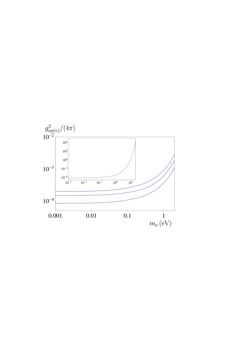
Figure 1: Constraints on the coupling constants of an axion to a proton or a neutron obtained from indirect measurements of the effective Casimir pressure versus the axion mass. The lines from bottom to top are plotted under the conditions $g_{ap}^{2}=g_{an}^{2}$, $g_{an}^{2}\gg g_{ap}^{2}$, and $g_{ap}^{2}\gg g_{an}^{2}$, respectively. In an inset the line is plotted under the condition $g_{ap}^{2}=g_{an}^{2}$ for larger masses. The regions of the plane above each line are prohibited and below each line are allowed.

We have found numerically (see Fig. 1) the values of the axion to nucleon coupling constants $g_{ap},\,g_{an}$ and masses $m_{a}$ satisfying the inequality (31). For this purpose, the expressions (27) and (29) were substituted in (31) over the mass intervals $10^{-2}\,\mbox{eV}<m_{a}<15\,$eV and $10^{-3}\,\mbox{eV}<m_{a}<10^{-2}\,$eV, respectively. We do not consider the axion masses $m_{a}<10^{-3}\,$eV because in this case the respective Compton wavelengths become too large and one cannot neglect the role of boundary effects (see Sec. 3). For $m_{a}>15\,$eV the constraints on $g_{ap}$ and $g_{an}$ following from this experiment become much weaker. In different intervals of $m_{a}$, the strongest constraints follow from the inequality (31) considered at different separation distances. Thus, for $m_{a}<0.1\,$eV the strongest constraints result at $a=300\,$nm and for $0.1\,\mbox{eV}\leq m_{a}<0.5\,$eV and $0.5\,\mbox{eV}\leq m_{a}<15\,$eV at $a=200\,$nm and 162 nm, respectively.

In Fig. 1, we present the obtained strongest constraints on the constants $g_{ap(n)}^{2}/(4\pi)$ as functions of the axion mass $m_{a}$. The lines correspond to the equality sign in (31). In Fig. 1 the three lines from bottom to top are plotted under the conditions $g_{ap}^{2}=g_{an}^{2}$, $g_{an}^{2}\gg g_{ap}^{2}$, and $g_{ap}^{2}\gg g_{an}^{2}$, respectively, for axion masses below 2 eV. The regions of the $(m_{a},g_{ap(n)}^{2})$ plane above each line are prohibited by the results of experiment 36 ; 37 , because the coordinates of their points violate inequality (31). The regions below each line are allowed by the results of this experiment. As can be seen in Fig. 1, for axions with masses $m_{a}<10^{-2}\,$eV the obtained constraints are almost independent of $m_{a}$. In an inset to Fig. 1 we plot the obtained constraints over a wider range of $m_{a}$ (up to 15 eV) under the condition $g_{ap}^{2}=g_{an}^{2}$. As is seen in this figure, with increasing $m_{a}$ the strength of constraints quickly decreases. In Table 2, we present the maximum allowed values of the axion-nucleon coupling constants over the most interesting region of masses from $m_{a}=10^{-3}\,$eV to 2 eV (column 1) partially overlapping with an axion window. The values in column 2 are obtained under the conditions $g_{ap}^{2}=g_{an}^{2}$, and columns 3 and 4 contain the maximum values of $g_{an}^{2}/(4\pi)$ and $g_{ap}^{2}/(4\pi)$ found under the conditions $g_{an}^{2}\gg g_{ap}^{2}$ and $g_{ap}^{2}\gg g_{an}^{2}$, respectively.

Table 2: Maximum values of the coupling constants of an axion to a proton and a neutron, allowed by indirect measurements of the Casimir pressure between Au plates, are calculated for different axion masses (column 1) under the conditions $g_{ap}^{2}=g_{an}^{2}$ (column 2), $g_{an}^{2}\gg g_{ap}^{2}$ (column 3), and $g_{ap}^{2}\gg g_{an}^{2}$ (column 4).

$m_{a}\,$(eV)	$\frac{g_{ap}^{2}}{4\pi}=\frac{g_{an}^{2}}{4\pi}$	$\frac{g_{an}^{2}}{4\pi}\gg\frac{g_{ap}^{2}}{4\pi}$	$\frac{g_{ap}^{2}}{4\pi}\gg\frac{g_{an}^{2}}{4\pi}$
$0.001$	$8.51\times 10^{-5}$	$1.49\times 10^{-4}$	$1.98\times 10^{-4}$
0.01	$8.74\times 10^{-5}$	$1.52\times 10^{-4}$	$2.04\times 10^{-4}$
0.05	$9.66\times 10^{-5}$	$1.67\times 10^{-4}$	$2.30\times 10^{-4}$
0.1	$1.08\times 10^{-4}$	$1.84\times 10^{-4}$	$2.59\times 10^{-4}$
0.2	$1.28\times 10^{-4}$	$2.16\times 10^{-4}$	$3.11\times 10^{-4}$
0.3	$1.48\times 10^{-4}$	$2.49\times 10^{-4}$	$3.62\times 10^{-4}$
0.4	$1.71\times 10^{-4}$	$2.88\times 10^{-4}$	$4.21\times 10^{-4}$
0.5	$1.96\times 10^{-4}$	$3.29\times 10^{-4}$	$4.85\times 10^{-4}$
0.6	$2.22\times 10^{-4}$	$3.73\times 10^{-4}$	$5.50\times 10^{-4}$
0.7	$2.51\times 10^{-4}$	$4.21\times 10^{-4}$	$6.24\times 10^{-4}$
0.8	$2.84\times 10^{-4}$	$4.76\times 10^{-4}$	$7.06\times 10^{-4}$
0.9	$3.21\times 10^{-4}$	$5.37\times 10^{-4}$	$7.97\times 10^{-4}$
1.0	$3.62\times 10^{-4}$	$6.05\times 10^{-4}$	$8.99\times 10^{-4}$
1.5	$6.48\times 10^{-4}$	$1.08\times 10^{-3}$	$1.61\times 10^{-3}$
2.0	$1.13\times 10^{-3}$	$1.88\times 10^{-3}$	$2.81\times 10^{-3}$

In Fig. 2(a) the constraints derived in this paper are compared with those found previously 19 ; 20 from measurements of the thermal Casimir-Polder force 48 and from experiments on measuring the gradient of the Casimir force between Au surfaces 21 ; 22 . For the sake of definiteness, the comparison is made under the most reasonable condition $g_{ap}^{2}=g_{an}^{2}$. The solid line in Fig. 2(a) reproduces the lower line in Fig. 1 obtained here. The dashed lines 1 and 2 reproduce the constraints obtained 19 ; 20 from measurements of the Casimir-Polder force and the gradient of the Casimir force over the regions of axion masses $m_{a}\leq 0.3\,$eV and $m_{a}\leq 1\,$eV, respectively. The regions of the plane above each line are prohibited and below each line are allowed by the results of the respective experiment.

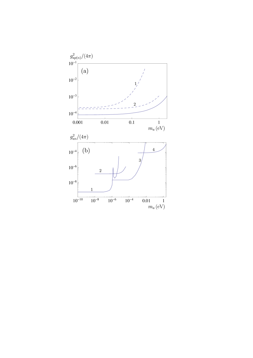
Figure 2: (a) Comparison between the constraints on the coupling constant of an axion to nucleon obtained here under the condition $g_{ap}^{2}=g_{an}^{2}$ (the solid line) with those obtained previously from experiments on measuring the thermal Casimir-Polder force (the dashed line 1) and the gradient of the Casimir force (the dashed line 2). The regions of the plane above each line are prohibited and below each line are allowed. (b) Constraints on the coupling constant $g_{an}$ following from magnetometer measurements 53a (the line 1), from the Cavendish-type experiments 17 ; 21a and 53b (the lines 2 and 3, respectively), and obtained in this work from measurements of the Casimir pressure by means of micromachined oscillator 36 ; 37 (the line 4).

As can be seen in Fig. 2(a), at $m_{a}=10^{-3}\,$eV and 1 eV our present constraints are stronger by the factors of 2.2 and 3.2, respectively, than those obtained from measurements of the gradient of the Casimir force (the dashed line 2). In comparison with the constraints from measurements of the Casimir-Polder force (the dashed line 1), the present constraints are stronger up to a factor of 380. This strengthening is achieved for the axion mass $m_{a}=0.3\,$eV.

Now we compare the obtained here strongest model-independent constraints on the coupling constant $g_{an}$ (the lower line in Fig. 1) with other model-independent constraints obtained to the present day. The line 1 in Fig. 2(b) shows the constraints found 53a with the help of a magnetometer using spin-polarized K and ³He atoms. These constraints are obtained in the region of axion masses from $10^{-10}$ to $6\times 10^{-6}\,$eV. The line 2 shows the constraints found in 18 from the Cavendish-type experiment 17 ; 21a for $m_{a}$ from $10^{-9}$ to $10^{-5}\,$eV. The results of a more modern Cavendish-type experiment 53b were used to constrain $g_{an}$ in the region from $m_{a}=10^{-6}\,$eV to $m_{a}=10^{-2}\,$eV 53c . These results are shown by the line 3 in Fig. 2(b). Our constraints obtained here are shown by the line 4. As is seen in Fig. 2(b), the model-independent constraints become weaker with increasing $m_{a}$ (the same takes place for the constraints on Yukawa-type corrections to Newtonian gravity arising from the exchange of scalar particles 29 ; 30 ; 31 ; 32 ; 33 ; 34 ; 35 ). It can be seen, however, that in the range of axion masses from $2\times 10^{-3}$ to 0.3 eV our constraints following from the Casimir effect are the strongest model-independent constraints.

A lot of constraints on an axion were obtained using some model approaches. Thus, the planar Si(Li) detector placed inside the low-background setup was used to detect the $\gamma$-quanta appearing in the deexcitation of the nuclear level excited by a solar axion 53d . In the framework of the model of hadronic axions, where the coupling constant is a function of the mass, the upper limits for the axion mass $m_{a}\leq 159\,$eV 53d and $m_{a}\leq 145\,$eV 53e were obtained. From the neutrino data of supernova SN 1987A it was found 53f that for the model of hadronic axions $g_{ap(n)}<10^{-10}$ or $g_{ap(n)}>10^{-3}$ with a narrow allowed region in the vicinity of $g_{ap(n)}=10^{-6}$. From astrophysical arguments connected with stellar cooling by the emission of hadronic axions a similar bound $g_{ap(n)}<3\times 10^{-10}$ was obtained 53g ; 53h . It should be noted, however, that the emission rate suffers from significant uncertainties related to dense nuclear matter effects 53h . In addition to a pseudoscalar coupling of axions to nucleons, it is possible also to introduce the scalar one 53i and consider respective coupling constants $g_{ap(n)}^{(s)}$. Several constraints on the product of constants $|g_{an}g_{an}^{(s)}|$ were obtained from experiments on neutron diffraction 53j . Thus, it was shown 53j that $|g_{an}g_{an}^{(s)}|<10^{-11}$ within the range of axion masses $2\times 10^{-5}\,\mbox{eV}<m_{a}<2\times 10^{3}\,$eV. When the axion mass increases up to $2\times 10^{6}\,$eV, the respective constraint becomes less stringent: $|g_{an}g_{an}^{(s)}|<10^{-7}$.

At the end of this section, we note that subsequent independent measurements of the gradient of the Casimir force in 21 ; 22 ; 23 ; 24 ; 25 confirmed both the experimental results of 36 ; 37 and their agreement with the Lifshitz theory under the condition that the low-frequency behavior of the dielectric permittivity of Au is described by the plasma model (the conclusion of 49 , claiming an agreement with the Drude model low-frequency behavior over the same range of separations was shown 50 to be based on an unaccounted systematic error).

6 Conclusions and discussion

In this paper we have derived stronger constraints on the pseudoscalar coupling constants of an axion to a proton and a neutron from measurements of the effective Casimir pressure by means of a micromachined oscillator. For this purpose, we have calculated the additional pressure between two parallel plates due to two-axion exchange and determined the validity region of the PFA when it is applied to the forces of axion origin. The role of boundary effects due to a finite area of the oscillator plate was determined.

The obtained constraints are applicable over a wide region of axion masses from $10^{-3}\,$eV to 15 eV, partially overlapping with an axion window. Under the assumption that $g_{ap}=g_{an}$, they are stronger up to a factor of 380 than the previously known laboratory constraints in this mass range derived from measurements of the thermal Casimir-Polder force and up to a factor of 3.15 than those found from measurements of the gradient of the Casimir force by means of AFM.

The obtained results demonstrate that measurements of the Casimir interaction using different laboratory techniques are useful in searching axion-like particles and constraining their coupling constants to nucleons. In future, it seems promising to consider the potentialities of more complicated experimental configurations, specifically, with corrugated boundary surfaces, for obtaining stronger constraints on the parameters of axion-like particles.

- (1) S. Weinberg, Phys. Rev. Lett. 40, 223 (1978).
- (2) F. Wilczek, Phys. Rev. Lett. 40, 279 (1978).
- (3) J. E. Kim, G. Carosi, Rev. Mod. Phys. 82, 557 (2010).
- (4) J. Beringer et al. (Particle Data Group), Phys. Rev. D 86, 010001 (2012).
- (5) R. D. Peccei, H. R. Quinn, Phys. Rev. Lett. 38, 1440 (1977).
- (6) K. Baker et al. Ann. Phys. (Berlin) 525, A93 (2013).
- (7) J. E. Kim, Phys. Rev. Lett. 43, 103 (1979).
- (8) M. A. Shifman, A. I. Vainstein, V. I. Zakharov, Nucl. Phys. B 166, 493 (1980).
- (9) A. P. Zhitnitskii, Sov. J. Nucl. Phys. 31, 260 (1980).
- (10) M. Dine, F. Fischler, M. Srednicki, Phys. Lett. B 104, 199 (1981).
- (11) Z. G. Berezhiani, M. Yu. Khlopov, Z.Phys. C — Particles and Fields 49, 73 (1991).
- (12) M. Khlopov, Fundamentals of Cosmic Particle Physics (CISP-Springer, Cambridge, 2012).
- (13) A. V. Derbin, S. V. Bakhlanov, I. S. Dratchnev, A. S. Kayunov, V. N. Muratova, Eur. Phys. J. C 73, 2490 (2013).
- (14) J. Jaeckel, E. Massó, J. Redondo, A. Ringwald, F. Takahashi, Phys. Rev. D 75, 013004 (2007).
- (15) P. Brax, C. van de Bruck, A.-C. Davis, Phys. Rev. Lett. 99, 121103 (2007).
- (16) J. E. Kim, Phys. Rep. 150, 1 (1987).
- (17) Yu. N. Gnedin, Int. J. Mod. Phys. A 17, 4251 (2002).
- (18) E. Fischbach, D. E. Krause, Phys. Rev. Lett. 82, 4753 (1999).
- (19) E. Fischbach, D. E. Krause, Phys. Rev. Lett. 83, 3593 (1999).
- (20) G. L. Smith, C. D. Hoyle, J. H. Gundlach, E. G. Adelberger, B. R. Heckel, H. E. Swanson, Phys. Rev. D 61, 022001 (1999).
- (21) J. H. Gundlach, G. L. Smith, E. G. Adelberger, B. R. Heckel, H. E. Swanson, Phys. Rev. Lett. 78, 2523 (1997).
- (22) R. Spero, J. K. Hoskins, R. Newman, J. Pellam, J. Schultz, Phys. Rev. Lett. 44, 1645 (1980).
- (23) J. K. Hoskins, R. D. Newman, R. Spero, J. Schulz, Phys. Rev. D 32, 3084 (1985).
- (24) E. G. Adelberger, E. Fischbach, D. E. Krause, R. D. Newman, Phys. Rev. D 68, 062002 (2003).
- (25) V. B. Bezerra, G. L. Klimchitskaya, V. M. Mostepanenko, C. Romero, Phys. Rev. D 89, 035010 (2014).
- (26) J. M. Obrecht, R. J. Wild, M. Antezza, L. P. Pitaevskii, S. Stringari, E. A. Cornell, Phys. Rev. Lett. 98, 063201 (2007).
- (27) V. B. Bezerra, G. L. Klimchitskaya, V. M. Mostepanenko, C. Romero, arXiv:1402.2528; Phys. Rev. D, to appear.
- (28) C.-C. Chang, A. A. Banishev, R. Castillo-Garza, G. L. Klimchitskaya, V. M. Mostepanenko, U. Mohideen, Phys. Rev. B 85, 165443 (2012).
- (29) A. A. Banishev, C.-C. Chang, R. Castillo-Garza, G. L. Klimchitskaya, V. M. Mostepanenko, U. Mohideen, Int. J. Mod. Phys. A 27, 1260001 (2012).
- (30) A. A. Banishev, C.-C. Chang, G. L. Klimchitskaya, V. M. Mostepanenko, U. Mohideen, Phys. Rev. B 85, 195422 (2012).
- (31) A. A. Banishev, G. L. Klimchitskaya, V. M. Mostepanenko, U. Mohideen, Phys. Rev. Lett. 110, 137401 (2013).
- (32) A. A. Banishev, G. L. Klimchitskaya, V. M. Mostepanenko, U. Mohideen, Phys. Rev. B 88, 155410 (2013).
- (33) G. L. Klimchitskaya, U. Mohideen, V. M. Mostepanenko, Rev. Mod. Phys. 81, 1827 (2009).
- (34) E. Fischbach, C. L. Talmadge, The Search for Non-Newtonian Gravity (Springer, New York, 1999).
- (35) I. Antoniadis, N. Arkani-Hamed, S. Dimopoulos, G. Dvali, Phys. Lett. B 436, 257 (1998).
- (36) M. Bordag, G. L. Klimchitskaya, U. Mohideen, V. M. Mostepanenko, Advances in the Casimir Effect (Oxford University Press, Oxford, 2009).
- (37) V. B. Bezerra, G. L. Klimchitskaya, V. M. Mostepanenko, C. Romero, Phys. Rev. D 81, 055003 (2010).
- (38) V. B. Bezerra, G. L. Klimchitskaya, V. M. Mostepanenko, C. Romero, Phys. Rev. D 83, 075004 (2011).
- (39) G. L. Klimchitskaya, U. Mohideen, V. M. Mostepanenko, Phys. Rev. D 86, 065025 (2012).
- (40) V. M. Mostepanenko, V. B. Bezerra, G. L. Klimchitskaya, C. Romero, Int. J. Mod. Phys. A 27, 1260015 (2012).
- (41) G. L. Klimchitskaya, U. Mohideen, V. M. Mostepanenko, Phys. Rev. D 87, 125031 (2013).
- (42) G. L. Klimchitskaya, V. M. Mostepanenko, Grav. Cosmol. 20, 3 (2014).
- (43) R. S. Decca, D. López, E. Fischbach, G. L. Klimchitskaya, D. E. Krause, V. M. Mostepanenko, Eur. Phys. J. C 51, 963 (2007).
- (44) R. S. Decca, D. López, E. Fischbach, G. L. Klimchitskaya, D. E. Krause, V. M. Mostepanenko, Phys. Rev. D 75, 077101 (2007).
- (45) C. D. Fosco, F. C. Lombardo, F. D. Mazzitelli, Phys. Rev. D 84, 105031 (2011).
- (46) L. P. Teo, M. Bordag, V. Nikolaev, Phys. Rev. D 84, 125037 (2011).
- (47) G. Bimonte, T. Emig, R. L. Jaffe, M. Kardar, Europhys. Lett. 97, 50001 (2012).
- (48) G. Bimonte, T. Emig, M. Kardar, Appl. Phys. Lett. 100, 074110 (2012).
- (49) L. P. Teo, Phys. Rev. D 88, 045019 (2013).
- (50) S. D. Drell, K. Huang, Phys. Rev. 91, 1527 (1953).
- (51) F. Ferrer, M. Nowakowski, Phys. Rev. D 59, 075009 (1999).
- (52) I. S. Gradshtein, I. M. Ryzhik, Table of Integrals, Series and Products (Academic Press, New York, 1980).
- (53) R. S. Decca, E. Fischbach, G. L. Klimchitskaya, D. E. Krause, D. López, V. M. Mostepanenko, Phys. Rev. D 79, 124021 (2009).
- (54) E. Fischbach, G. L. Klimchitskaya, D. E. Krause, V. M. Mostepanenko, Eur. Phys. J. C 68, 223 (2010).
- (55) E. M. Lifshitz, L. P. Pitaevskii, Statistical Physics, Part II (Pergamon, Oxford, 1980).
- (56) G. Vasilakis, J. M. Brown, T. R. Kornack, M. V. Romalis, Phys. Rev. Lett. 103, 261801 (2009).
- (57) D. J. Kapner, T. S. Cook, E. G. Adelberger, J. H. Gundlach, B. R. Heckel, C. D. Hoyle, H. E. Swanson, Phys. Rev. Lett. 98, 021101 (2007).
- (58) E. G. Adelberger, B. R. Heckel, S. Hoedl, C. D. Hoyle, D. J. Kapner, A. Upadhye, Phys. Rev. Lett. 98, 131104 (2007).
- (59) A. V. Derbin, A. L. Frolov, L. A. Mitropol’sky, V. N. Muratova, D. A. Semenov, E. V. Unzhakov, Eur. Phys. J. C 62, 755 (2009).
- (60) A. V. Derbin, V. N. Muratova, D. A. Semenov, E. V. Unzhakov, Phys. Atom. Nucl. 74, 596 (2011).
- (61) J. Engel, D. Seckel, A. C. Hayes, Phys. Rev. Lett. 65, 960 (1990).
- (62) W. C. Haxton, K. Y. Lee, Phys. Rev. Lett. 66, 2557 (1991).
- (63) G. Raffelt, Phys. Rev. D 86, 015001 (2012).
- (64) J. E. Moody, F. Wilczek, Phys. Rev. D 30, 130 (1984).
- (65) V. V. Voronin, V. V. Fedorov, I. A. Kuznetsov, JETP Lett. 90, 5 (2009).
- (66) D. Garcia-Sanches, K. Y. Fong, H. Bhaskaran, S. Lamoreaux, H. X. Tang, Phys. Rev. Lett. 109, 027202 (2012).
- (67) M. Bordag, G. L. Klimchitskaya, V. M. Mostepanenko, Phys. Rev. Lett. 109, 199701 (2012).