Distinguishing orbital angular momenta and topological charge in optical vortex beams

Abstract

In this work we discuss how the classical orbital angular momentum (OAM) and topological charge (TC) of optical beams with arbitrary spatial phase profiles are related to the local winding density. An analysis for optical vortices (OV) with non-cylindrical symmetry is presented and it is experimentally shown for the first time that OAM and TC may have different values. The new approach also provides a systematic way to determine the uncertainties in measurements of TC and OAM of arbitrary OV.

Optical vortices (OV) have been extensively studied since the seminal work by Allen et al. (allenorbital1992, ) and are applied in topics as diverse as classical and quantum communications (WillnerTerabitTelecom2012, ; ZeillingerOAMentanglement2001, ; plickquantum2013, ), optical tweezers (Ritsh-Marte2008, ; DholakiaPerfectVortexDynamics2013, ) and plasmonics (Lee2010, ; rurycoherent2013, ; toyodaOVtwistednanostructures2012, ; gorodetskiOAMfromPlasmon2013, ; brasselettopological2013, ). However, there are subtleties in characterizing such optical beams that are not usually remarked. Canonical OV, as associated to Bessel or Laguerre-Gauss beams, carry well defined mean values of orbital angular momentum (OAM) and topological charge (TC). In these cases, the OAM per photon and the TC have the same value. However, by analyzing these quantities for non-canonical OV it can be seen that they represent distinct quantities. A proper understanding of non-canonical OV is of great interest because they extend the current applications of OV. For example, it is possible to control transverse forces in optical tweezers (Ritsh-Marte2008, ), or increase the excitation efficiency of surface plasmon modes (brasselettopological2013, ). In the present work we explicitly distinguish classical and modal OAM and TC for arbitrarily shaped OV beams. This is fundamental to avoid mistakes when analyzing the experimental consequences of more general beams.

Diffractive and interferometric techniques as (soskintopological1997, ; berkhoutmultipinhole2008, ; Hickmann2010, ) are sensitive to the phase profile, hence they measure the total topological charge (TC) of a beam. The quantum OAM distribution may be obtained via diffractive elements (PadgettOAMSorting2010, ; BoydOAMSorting2013, ) or modal decomposition (LofflerOAMsidebands2012, ; ForbesModeDecomposition2013, ). The classical OAM of a light beam may be determined by measuring the electric field amplitude and phase, as in (Padgettfractionavortex2004, ), or also via modal decomposition (ForbesModeDecomposition2013, ).

We consider a scalar OV beam under the paraxial approximation. In cylindrical coordinates $\mathbf{r}=\mathbf{r}\left(\rho,\phi,z\right)$ a linearly polarized and monochromatic field in vacuum may be represented by the following vector potential

$$\mathbf{A}\left(\mathbf{r},t\right)=\hat{\epsilon}\left(\frac{2\mu_{0}}{\omega k}P_{0}\right)^{\frac{1}{2}}\mathcal{A}\left(\mathbf{r}\right)\exp i\left[\chi\left(\mathbf{r}\right)+kz-\omega t\right],$$ (1)

where $P_{0}$ is the optical power, $\mu_{0}$ is the vacuum permeability, $\omega,k$ are respectively the angular frequency and wave number of light. The remaining terms are the beam phase profile $\chi\left(\mathbf{r}\right)$ and $\mathcal{A}\left(\mathbf{r}\right)$ is the vector potential amplitude envelope, normalized such that $\int d^{2}r\left|\mathcal{A}\left(\mathbf{r}\right)\right|^{2}=1$. The total TC, $Q_{T}$, contained inside a contour $C$ of radius $c$, on the $\rho\phi$ plane, is given by (Nakahara, ; Berry2004, )

$$Q_{T} =\frac{1}{2\pi}\oint_{C}d\mathbf{x}\cdot\nabla\chi\left(\mathbf{r}\right)=\frac{1}{2\pi}\int_{0}^{2\pi}w\left(\rho=c,\phi\right)d\phi,$$ (2)

where the local winding density (LWD) $w\left(\mathbf{r}\right)$ is a quantity that gives the local effect of the TC, is defined by

$$w\left(\mathbf{r}\right)=\frac{\partial\chi}{\partial\phi}\left(\mathbf{r}\right).$$ (3)

The total TC gives the number of times that the beam phase pass through the interval $\left[0,2\pi\right]$ following the curve $C$. For a well-behaved contour, $Q_{T}$ is an integer even if $\chi\left(\mathbf{r}\right)$ is discontinuous (Berry2004, ).

On the other hand, the classical OAM density along the propagation direction $\hat{z}$ is $L_{z}=\frac{\epsilon_{0}\omega}{2}\mathfrak{Re}\left\{\mathbf{A}\left(\mathbf{r},t\right)\left(-i\frac{\partial}{\partial\phi}\right)\mathbf{A}^{*}\left(\mathbf{r},t\right)\right\}$ (Berryparaxialbeams1998, ), and it may be shown by direct substitution of eq. (1) that

$$L_{z}=\frac{P_{0}}{\omega c}\left[\mathcal{A}^{*}\left(\mathbf{r}\right)\frac{\partial\chi}{\partial\phi}\mathcal{A}\left(\mathbf{r}\right)\right].$$ (4)

Since $P_{0}=N\hbar\omega$, where $N$ is the number of photons impinging on the plane $\rho\phi$ per second carrying energy $\hbar\omega$, the local OAM value per photon at a given position is (PadgettMathieu2002, ) $\hbar w=\hbar\partial\chi/\partial\phi$. So, the LWD gives the local OAM per photon.

We remark that although the intensity profile of a beam is related to its TC distribution (Berry2004, ; Grier2003, ; Shaping_Optical_Beams, ), the intensity profile carries no information about the topological or OAM properties of a beam (pugatchtopological2007, ).

Since the product $\mathcal{A}^{*}\left(\mathbf{r}\right)\mathcal{A}\left(\mathbf{r}\right)$ gives the probability of finding a photon at a given point, the average classical OAM per photon may be determined from eq. (4) as (PadgettMathieu2002, )

$$\hbar\left\langle l\right\rangle_{class.}=\hbar\int d^{2}r\mathcal{A}^{*}\left(\mathbf{r}\right)\frac{\partial\chi}{\partial\phi}\mathcal{A}\left(\mathbf{r}\right).$$ (5)

A comparison between eqs. (2) and (5) shows that only in very specific situations $Q_{T}=\left\langle l\right\rangle_{class.}$. An immediate result is that measuring $Q_{T}$ one does not necessarily have information about $\left\langle l\right\rangle_{class.}$ and vice-versa. However, both quantities are related to the LWD which can be obtained from $\chi\left(\mathbf{r}\right)$. Therefore we emphasize that it is important to determine the LWD for the characterization of the classical OAM and TC in OV beams.

In a quantum description of OAM, it can be shown that eq. (5) gives the correct average OAM . Thus, if $\left|p,m\right\rangle$ represents the radial and azimuthal quantum numbers $p$ and $m$, respectively, it can be seen that the average OAM is given by

$$\hbar\left\langle l\right\rangle_{quant.}=\hbar\sum_{p,m}m\left|\left\langle\mathcal{A}|p,m\right\rangle\right|^{2},$$ (6)

while a comparison with the classical expression, eq. (5), shows that, as expected by the correspondence principle, $\hbar\left\langle l\right\rangle_{quant.}=\hbar\left\langle l\right\rangle_{class.}$ and then [34]

$$\hbar\int d^{2}r\mathfrak{Re}\left\{\left\langle\mathcal{A}|\mathbf{r}\right\rangle\hat{L}_{z}\left\langle\mathbf{r}|\mathcal{A}\right\rangle\right\}=\hbar\left\langle l\right\rangle_{class.}.$$ (7)

The setup shown in Fig. 1 allows a full characterization of a linearly polarized electric field by measuring its amplitude and phase. It consists of a Michelson interferometer in which Arm 1 contains a spatial light modulator (SLM). When Arm 2 is blocked, only the intensity profile will be detected by the CCD, otherwise an interference pattern will be detected. From the interference pattern, $\chi\left(\mathbf{r}\right)$ may be retrieved using Fourier transforms (Takeda-Fourier-transform1982, ). To obtain a better signal/noise ratio, we averaged the phase for 20 applied constant phase offsets on the SLM (Padgettfractionavortex2004, ). To compute the azimuthal derivative in the LWD, we used a Fourier spectral method with a smoothing gaussian filter (ahnertnumerical2007, ). To determine $w\left(\mathbf{r}\right)$, we used the following identity $w\left(\mathbf{r}\right)=\partial\chi/\partial\phi=e^{-i\chi}\left[-i\left(x\frac{\partial}{\partial y}-y\frac{\partial}{\partial x}\right)\right]e^{i\chi}.$

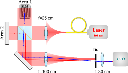
Figure 1: Experimental setup (not to scale). The output of a fiber coupled laser diode emitting at $805$ nm is collimated with a lens with long focal distance ($f=25$ cm), producing a nearly plane wave. The collimated light goes to a Michelson interferometer in which the arm 1 contains a SLM (Hamamatsu - LCOS X10468-02). The arm 2 provides the plane wave reference, and it is blocked when beam intensity measurements are performed. The reference (red) and modulated (blue) beams have a small relative angle and are spatially filtered and then imaged on a CCD camera (Coherent - Lasercam HR) positioned at the SLM image plane.

The first set of measurements was obtained with beams having a linear azimuthal phase dependence $\chi_{sig}=\alpha\phi$, for integer $\alpha$. For all measurements, the SLM phase profile was composed of $\chi_{sig}$, a circular aperture with fixed radius and a carrier wave. A typical $\chi_{sig}$ is shown in Fig. 2 (a) for $\alpha=10$. The measured amplitude and phase profiles are shown, respectively in Figs. 2 (b-c) and the corresponding LWD is shown in Fig. 2 (d). Notice that, as expected, $w\left(\mathbf{r}\right)$ is well defined along the beam profile, except where the intensity is very small and the phase is not well retrieved. Outside the beam intense region there is a background due to light diffracted from the SLM which adds systematic phase and LWD shifts.

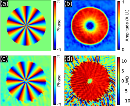
Figure 2: (color online) Typical profiles for a vortex with azimuthal phase $\chi_{sig}=10\phi$. (a) Phase pattern applied to the SLM (without carrier). (b) and (c) contains, respectively, the experimentally measured amplitude and phase profiles, averaged in 20 samples. Notice that the experimental phase profile (d) agree well with the phase applied at the SLM (a). (d) Spatial profile of the LWD.

For a quantitative description of the classical OAM and the TC, we notice that eq. (2) can be considered as an average of the LWD over a narrow ring and (5) is an average of the LWD weighted by $\left|\mathcal{A}\right|^{2}$. So, weighting the LWD with $K^{\mbox{TC}}=1$ over a ring ($K^{\mbox{OAM}}=\left|\mathcal{A}\right|^{2}$ over the beam) one may build histograms representing the probability $P^{\mbox{TC}}$ ($P^{\mbox{OAM}}$) of finding a given value $w^{\prime}$ of LWD (OAM) in a narrow range, $\epsilon\ll 1$, and whose average is $Q_{T}$ ($\left\langle l\right\rangle_{class.}$) via

$$P^{\beta}\left(w^{\prime}\right) =\frac{\int d^{2}r\,\theta\left[\epsilon-\left|w\left(\mathbf{r}\right)-w^{\prime}\right|\right]K^{\beta}}{\int d^{2}r\,K^{\beta}},$$ (8)

where $\theta$ is the step function and $\beta$ corresponds to TC or OAM.

The TC and classical OAM histograms, as defined above, allow quantitative determination of the uncertainties of the measured quantities. To the best of our knowledge, no previous classical characterization of OAM and TC was able to determine these uncertainties. We also produced histograms for the modal OAM distribution, which is related to the quantum OAM, by expanding the field in a basis of Bessel functions. It can be seen in Fig. 3 (a) that $\left\langle Q_{T}\right\rangle$, $\left\langle l\right\rangle_{class.}$ and $\left\langle l\right\rangle_{modal}$ are similar for integer $\alpha$. The associated histograms for each $\alpha$ can be seen in Figs. 3 (b-d). Except for the distinction of quasi-continuous distribution in Figs. 3 (b-c) for TC and classical OAM and the discrete distribution for modal OAM, no major differences are observed.

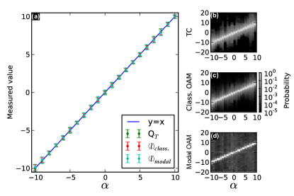
Figure 3: (color online) (a) Superimposed plots of measured TC, classical OAM via (5) and modal OAM via full mode decomposition, eq. (6). No distinction is observed for all quantities. (b), (c) and (d) are, respectively, the histograms associated with TC, classical OAM and modal OAM. The curve $y=x$ is added as a visual guide.

On the other hand, TC and OAM for fractional values of $\alpha$ behave differently from integer ones. As suggested in (Berry2004, ), $Q_{T}$ is the nearest integer to $\alpha$. Simultaneously, it can be shown that the OAM for fractional $\alpha$ is $\left\langle l\right\rangle=\alpha-\sin\left(2\pi\alpha\right)/2\pi$ (Padgettfractionavortex2004, ; BarnettQuantumFractionalOV2007, ). The experimental histograms for OAM and TC are shown in Figs. 4 (a,c,e). In Fig. 4 (a) it is shown how $\left\langle Q_{T}\right\rangle$ varies with $\alpha$. In Figs. 4 (c,e) it can be seen that $\left\langle l\right\rangle$ follows smoothly the theoretical prediction. The insets in Fig. 4 (a, c, e) exhibit respectively, the LWD profile (eq. (3)), and local probability densities for classical OAM (integrand of eq. (5)) and modal OAM (integrand of eq. (6) obtained from the Bessel expansion). We remark that modal OAM histogram also behaves as is theoretically expected (BarnettQuantumFractionalOV2007, ).

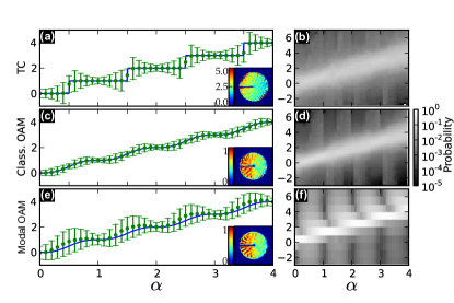
Figure 4: (color online) Experimental determination of TC (a), classical OAM via eq. (5) (c) and modal OAM via eq. (6) (e). The insets contain the spatial profiles of the LWD (a), and the classical OAM density profile obtained from classical and modal expressions (c, e) for $\alpha=2.5$. The theoretical predictions are represented by continuous lines. (b), (d) and (f) correspond, respectively, to the histograms for the TC, classical OAM and modal OAM.

In Fig. 5 we consider Lissajous-shaped OV, in which the OV cores form Lissajous patterns (Grier2003, ). The phase and LWD profiles of these OV may be written respectively as$\chi_{\mbox{Lissajous}}=l\phi+a\sin\left(j\phi\right)/j$ and $w_{\mbox{Lissajous}}=l+a\cos(j\phi)$, with $j\neq 0$.

Since the oscillatory term averages to zero, it is expected that $\left\langle Q_{T}\right\rangle=\left\langle l\right\rangle=l$, and this can be observed in Figs. 5 (a, d, g). Notice that, the histograms for $l=5$ in Fig. 5 (c, f, i) are shifted with respect to those with $l=0$ in Fig. 5 (b, e, h). An interesting feature of Lissajous OV is in the comparison between the classical and modal OAM. Approximating the beam by a top-hat, the classical OAM histogram is not sensitive to the number of $w$ oscillations. Therefore it depends only on $l$ and $a$ as is observed for $j\neq 0$ in Figs. 5 (e, f). Meanwhile, the modal OAM depends on $j$, as seen in Figs. 5 (h, i) and from the probability of obtaining the OAM eigenvalue $l^{\prime}$ in a Lissajous OV in terms of Bessel functions $P\left(l^{\prime}\right)=\left|J_{\frac{l^{\prime}-l}{j}}\left(\frac{a}{j}\right)\right|^{2}$ (Gradshteyn, ).

Notice that the different $j$ dependence between the classical and modal OAM of Lissajous OV may be used to distinguish classical and quantum OAM transfer.

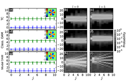
Figure 5: (color online) (a, d, g) TC, classical OAM and modal OAM for Lissajous OV with $a=5$ and $l=0$ (blue) or $l=5$ (green). Solid lines represent the theoretically expected values. The insets contain the spatial profiles of the LWD (a), and the classical OAM density profile obtained from classical and modal expressions (d, g) for $l=0,\,j=3$. (b, e, h) Histograms of TC, classical OAM and modal OAM for $l=0$. (c, f, i) Histograms of TC, classical OAM and modal OAM for $l=5$.

Finally we consider a linear distribution of OV, each having a unitary TC (Shaping_Optical_Beams, ). The OV are uniformly spaced over a line of length $b$ and inside a circular intensity envelope of diameter $D$. It can be shown that using such distribution of TCs one may shape the OV core for small TC separation (Shaping_Optical_Beams, ). The experimental results are shown in Fig. 6. As a first remark, it may be noticed that, since the total TC is the sum of the individual TCs, it remains constant for all $b/D$ values in Fig. 6 (a). The TC histogram in Fig. 6 (b), varies little with $b/D$ and essentially becomes slightly broader for larger $b/D$. A different behavior is observed for the OAM. For large $b/D$ values, the average OAM is reduced because the phase due to each OV is compensated between equally charged vortices and such regions become more illuminated for larger TC separations. This fact can also be seen from a full description of such TC distribution (Indebetouw1993, ). The classical and modal OAM histograms of Figs. 6 (d, f) have similar profiles, the modal one being grainier. The similarity in this non-cyllindrical OV configuration is interesting because it corroborates the correctness of our interpretation of eq. (8) as a classical probability of finding a given OAM in a light beam.

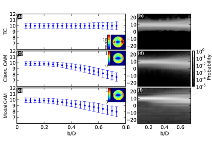
Figure 6: (color online) Line of equally charged OV for $D=3.3$ mm. (a) Total TC, (c,e) classical and modal OAM. On insets are represented the spatial profiles of the LWD (a), and the classical OAM density profile obtained from classical and quantum expressions (c, e) for $b/D=0.6$. In (b,d,f) are represented the histograms respective to (a,c,e).

In summary, we remark that by analysis of the LWD one may obtain spatial information about the TC and the classical OAM content of a light beam. The characterization presented is applicable to arbitrarily shaped OV and clarifies that TC and OAM are usually different quantities. Such distinction is important because it raises fundamental questions. For example, are the increased coherence storage times for OV reported in (pugatchtopological2007, ) due to TC or OAM? Does the excitation of surface plasmons in (Lee2010, ; toyodaOVtwistednanostructures2012, ; gorodetskiOAMfromPlasmon2013, ; brasselettopological2013, ) depends on mode matching (modal OAM), or phase matching (classical OAM)? Is it possible to observe quantum OAM transfer in an optical tweezer? Although we have indications that the integrand of eq. (5) is a classical probability of finding a given OAM value, a proper verification could be given by obtaining angular velocity histograms in an optical tweezer setup as (DholakiaPerfectVortexDynamics2013, ; DholakiaOAMMathieubeams2006, ; RaizenTweezerinVacuum2011, ). Also, the proposed histograms are amenable to theoretical modelling, that can be used to retrieve quantitatively the experimental parameters of shaped OV beams and their uncertainties. A final remark is that eq. (5) allows a much simpler and faster way to calculate the average OAM for a beam with known amplitude and phase profile than decomposing it in a basis of OAM eigenmodes.

We acknowledge the financial support from the Brazilian agencies CNPq (INCT-Fotônica) and FACEPE. We also acknowledge helpful discussions with Dr. L. Pruvost. A. M. A. also thanks Dr. W. Löffler for inciting an extension of our work on shaped OV (Shaping_Optical_Beams, ).

Supplementary informations

We consider a complete basis of OAM eigenfunctions labelled by $p$ and $m$ as, respectively the radial and the azimuthal quantum numbers. Using the completeness relation $1=\sum_{p,m}\left|p,m\left\rangle\right\langle p,m\right|$ it may be shown that the average OAM is

$$\left\langle L_{z}\right\rangle=\left\langle\mathcal{A}\left|\hat{L}_{z}\right|\mathcal{A}\right\rangle=\sum_{p,m}m\left|\left\langle\mathcal{A}|p,m\right\rangle\right|^{2}.$$ (9)

Meanwhile, one may express the average in terms of spatial wave functions $\mathcal{A}\left(\mathbf{r}\right)=\left\langle\mathbf{r}|\mathcal{A}\right\rangle$.

$$\left\langle L_{z}\right\rangle =\int d^{2}r\left\langle\mathcal{A}|\mathbf{r}\right\rangle\left\langle\mathbf{r}\left|\hat{L}_{z}\right|\mathcal{A}\right\rangle,$$ (10)

$$=\int d^{2}r\left\langle\mathcal{A}|\mathbf{r}\right\rangle\hat{L}_{z}\left\langle\mathbf{r}|\mathcal{A}\right\rangle.$$ (11)

Since $\left\langle L_{z}\right\rangle$ is real, the imaginary part of the integrand in Eq. (11) must cancel. Therefore the classical OAM density is given by

$$\left\langle L_{z}\right\rangle\left(\mathbf{r}\right)=\mathfrak{Re}\left\{\left\langle\mathcal{A}|\mathbf{r}\right\rangle\hat{L}_{z}\left\langle\mathbf{r}|\mathcal{A}\right\rangle\right\},$$ (12)

or, by expanding $\left|\mathcal{E}\right\rangle$ in the OAM eigenfunctions,

$$\left\langle L_{z}\right\rangle\left(\mathbf{r}\right)=\mathfrak{Re}\left\{\sum_{\begin{array}[]{c}p,m\\ p^{\prime},m^{\prime}\end{array}}m\left\langle\mathcal{A}|p,m\right\rangle\left\langle p^{\prime},m^{\prime}|\mathcal{A}\right\rangle\left\langle\mathbf{r}|p^{\prime},m^{\prime}\right\rangle\left\langle p,m|\mathbf{r}\right\rangle\right\}.$$ (13)

Equation (12) may also be expressed in terms of the beam phase profile. Using that $\hat{L}_{z}=-i\frac{\partial}{\partial\phi}$ and expressing $\left\langle\mathbf{r}|\mathcal{A}\right\rangle=\left|\mathcal{A}\right|\exp\left(i\chi\right)$, it is possible to show that

$$\left\langle L_{z}\right\rangle\left(\mathbf{r}\right)=\left\langle\mathcal{A}|\mathbf{r}\right\rangle\frac{\partial\chi}{\partial\phi}\left\langle\mathbf{r}|\mathcal{A}\right\rangle.$$ (14)

Equations (13) and (14) are, respectively, the expressions used to represent the classical OAM density profile from the modal and classical data in Figs. 4-6.

References

- (1) L. Allen, M. W. Beijersbergen, R. J. C. Spreeuw, and J. P. Woerdman, Phys. Rev. A 45, 8185 (1992).
- (2) J. Wang, J. Yang, I. M. Fazal, N. Ahmed, Y. Yan, H. Huang, Y. Ren, Y. Yue, S. Dolinar, M. Tur, and A. E. Willner, Nature Photon. 6, 488 (2012).
- (3) A. Mair, A. Vaziri, G. Weihs, and A. Zeilinger, Nature 412, 313 (2001).
- (4) W. N. Plick, M. Krenn, R. Fickler, S. Ramelow, and A. Zeilinger, Phys. Rev. A 87, 033806 (2013).
- (5) A. Jesacher, C. Maurer, S. Fuerhapter, A. Schwaighofer, S. Bernet, and M. Ritsch-Marte, Opt. Commun. 281, 2207 (2008).
- (6) M. Chen, M. Mazilu, Y. Arita, E. Wright, and K. Dholakia, Opt. Lett. 38, 4919 (2013).
- (7) H. Kim, J. Park, S.-W. Cho, S.-Y. Lee, M. Kang, and B. Lee, Nano Lett. 10, 529 (2010).
- (8) A. Rury, Phys. Rev. B 88, 205132 (2013).
- (9) K. Toyoda, K. Miyamoto, N. Aoki, R. Morita, and T. Omatsu, Nano Lett. 12, 3645 (2012).
- (10) Y. Gorodetski, A. Drezet, C. Genet, and T. W. Ebbesen, Phys. Rev. Lett. 110, 203906 (2013).
- (11) E. Brasselet, G. Gervinskas, G. Seniutinas, and S. Juodkazis, Phys. Rev. Lett. 111, 193901 (2013).
- (12) M. Soskin, V. Gorshkov, M. Vasnetsov, J. Malos, and N. Heckenberg, Phys. Rev. A 56, 4064 (1997).
- (13) G. Berkhout and M. Beijersbergen, Phys. Rev. Lett. 101, 100801 (2008).
- (14) J. M. Hickmann, E. J. S. Fonseca, W. C. Soares, and S. Chávez-Cerda, Phys. Rev. Lett. 105, 053904 (2010).
- (15) G. Berkhout, M. Lavery, J. Courtial, M. Beijersbergen, and M. Padgett, Phys. Rev. Lett. 105, 153601 (2010).
- (16) M. Mirhosseini, M. Malik, Z. Shi, and R. Boyd, Nature comm. p. 4:2781 (2013).
- (17) W. Löffler, A. Aiello, and J. P. Woerdman, Phys. Rev. Lett. 109, 113602 (2012).
- (18) C. Schulze, A. Dudley, D. Flamm, M. Duparré, and A. Forbes, New J. Phys. 15, 073025 (2013).
- (19) J. Leach, E. Yao, and M. Padgett, New J. Phys. 6, 71 (2004).
- (20) M. Nakahara, Geometry, Topology and Physics (Taylor & Francis, 2003).
- (21) M. V. Berry, J. Opt. A: Pure Appl. Opt. 6, 259 (2004).
- (22) M. V. Berry, Proc. SPIE 3487, 6 (1998).
- (23) S. Chávez-Cerda, M. Padgett, I. Allison, G. New, J. Gutiérrez-Vega, A. O’Neil, I. MacVicar, and J. Courtial, J. Opt. B: Quantum and Semiclass. Opt. 4, S52 (2002).
- (24) J. E. Curtis and D. G. Grier, Opt. Lett. 28, 872 (2003).
- (25) A. M. Amaral, E. L. Falcão-Filho, and C. B. de Araújo, Opt. Lett. 38, 1579 (2013).
- (26) R. Pugatch, M. Shuker, O. Firstenberg, A. Ron, and N. Davidson, Phys. Rev. Lett. 98, 203601 (2007).
- (27) M. Takeda, H. Ina, and S. Kobayashi, J. Opt. Soc. Am. 72, 156 (1982).
- (28) K. Ahnert and M. Abel, Comput. Phys. Commun. 177, 764 (2007).
- (29) J. Götte, S. Franke-Arnold, R. Zambrini, and S. M. Barnett, J. Mod. Opt. 54, 1723 (2007).
- (30) I. S. Gradshteyn and I. M. Ryzhik, Table of integrals, series, and products (Academic Press, 2007).
- (31) G. Indebetouw, J. Mod. Opt. 40, 73 (1993).
- (32) L. Carlos, G. Julio, G. Milne, and K. Dholakia, Opt. Express 14, 4183 (2006).
- (33) T. Li, S. Kheifets, and M. Raizen, Nature Phys. 7, 527 (2011).