Wavefront sensing reveals optical coherence

Abstract

Wavefront sensing is a set of techniques providing efficient means to ascertain the shape of an optical wavefront or its deviation from an ideal reference. Due to its wide dynamical range and high optical efficiency, the Shack-Hartmann is nowadays the most widely used of these sensors. Here, we show that it actually performs a simultaneous measurement of position and angular spectrum of the incident radiation and, therefore, when combined with tomographic techniques previously developed for quantum information processing, the Shack-Hartmann can be instrumental in reconstructing the complete coherence properties of the signal. We confirm these predictions with an experimental characterization of partially coherent vortex beams, a case that cannot be treated with the standard tools. This seems to indicate that classical methods employed hitherto do not fully exploit the potential of the registered data.

Light is a major carrier of information about the universe around us, from the smallest to the largest scale. Three-dimensional objects emit radiation that can be viewed as complex wavefronts shaped by diverse features, such as refractive index, density, or temperature of the emitter. These wavefronts are specified by both their amplitude and phase; yet, as conventional optical detectors measure only (time-averaged) intensity, information on the phase is discarded. This information turns out to be valuable for a variety of applications, such as optical testing Malacara:2007kx , image recovery Dai:2008zr , displacement and position sensing Ares:2000fk , beam control and shaping Katz:2011ly ; McCabe:2011ij ; Mosk:2012bs , as well as active and adaptive control of optical systems Tyson:2011ys , to mention but a few.

Actually, there exists a diversity of methods for wavefront reconstruction, each one with its own pros and cons Geary:1995fk . Such methods can be roughly classified into three categories: (a) interferometric methods, based on the superposition of two beams with a well-defined relative phase; (b) methods based on the measurement of the wavefront slope or wavefront curvature, and (c) methods based on the acquisition of images followed by the application of an iterative phase-retrieval algorithm Luke:2002ad . Notwithstanding the enormous progress that has already been made, practical and robust wavefront sensing still stands as an unresolved and demanding problem Campbell:2006if .

The time-honored example of the Shack-Hartmann (SH) wavefront sensor surely deserves a special mention Platt:2001dz : its wide dynamical range, high optical efficiency, white light capability, and ability to use continuous or pulsed sources make of this setup an excellent solution in numerous applications.

The operation of the SH sensor appeals to the intuition, giving the overall impression that the underlying theory is obvious Primot:2003fe . Indeed, it is often understood in an oversimplified geometrical-optics framework, which is much the same as assuming full coherence of the detected signal. By any means, this is not a complete picture: even in the simplest instance of beam propagation, the coherence features turn out to be indispensable Mandel:1995qy .

It has been recently suggested Hradil:2010fv that SH sensing can be reformulated in a concise quantum notation. This is more than an academic curiosity, because it immediately calls for the application of the methods of quantum state reconstruction lnp:2004uq . Accordingly, one can verify right away that wavefront sensors may open the door to an assessment of the mutual coherence function, which conveys full information on the signal.

In this paper, we report the first experimental measurement of the coherence properties of an optical beam with a SH sensor. To that end, we have prepared several coherent and incoherent superpositions of vortex beams. Our strategy can efficiently disclose that information, whereas the common SH operation fails in the task.

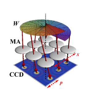
Figure 1: The principle of the SH wavefront sensor. A microlens array (MA) subdivides the wavefront ($W$) into multiple beams that are focused in a CCD camera. Local slope of the wavefront over each microlens aperture determines the location of the spot on the CCD. Red arrows represent normals to the wavefront.

Results

SH wavefront sensing. The working principle of the SH wavefront sensor can be elaborated with reference to Fig. 1. An incoming light field is divided into a number of sub-apertures by a microlens array that creates focal spots, registered in a CCD camera. The deviation of the spot pattern from a reference measurement allows the local direction angles to be derived, which in turn enables the reconstruction of the wavefront. In addition, the intensity distribution within the detector plane can be obtained by integration and interpolation between the foci.

Unfortunately, this naive picture breaks down when the light is partially coherent, because the very notion of a single wavefront becomes somewhat ambiguous: the signal has to be conceived as a statistical mixture of many wavefronts Goodman:2005qa . To circumvent this difficulty, we observe that these sensors provide a simultaneous detection of position and angular spectrum (i.e., directions) of the incident radiation. In other words, the SH is a pertinent example of a simultaneous unsharp position and momentum measurement, a question of fundamental importance in quantum theory and about which much has been discussed Arthurs:1965pi ; Stenholm:1992lh ; Raymer:1994ye .

Rephrasing the SH operation in a quantum parlance will prove pivotal for the remaining discussion. Let $\varrho$ be the coherence matrix of the field to be analyzed. Using an obvious Dirac notation, we can write $G(\mathbf{x}^{\prime},\mathbf{x}^{\prime\prime})=\langle\mathbf{x}^{\prime}|\varrho|\mathbf{x}^{\prime\prime}\rangle=\mathop{\mathrm{Tr}}\nolimits(\varrho|\mathbf{x}^{\prime}\rangle\langle\mathbf{x}^{\prime\prime}|)$, where $|\mathbf{x}\rangle$ is a vector describing a point-like source located at $\mathbf{x}$ and $\mathop{\mathrm{Tr}}\nolimits$ is the matrix trace. Thereby, the mutual coherence function $G(\mathbf{x}^{\prime},\mathbf{x}^{\prime\prime})$ appears as the position representation of the coherence matrix. As a special case, the intensity distribution across a transversal plane becomes $I(\mathbf{x})=\mathop{\mathrm{Tr}}\nolimits(\varrho|\mathbf{x}\rangle\langle\mathbf{x}|)$. Moreover, a coherent beam of complex amplitude $U(\mathbf{x})$, can be assigned to a ket $|{U}\rangle$, such that $U(\mathbf{x})=\langle\mathbf{x}|U\rangle$.

To simplify, we restrict the discussion to one dimension, denoted by $x$. If the setup is illuminated with a coherent signal $U(x)$, and the $i$th microlens is $\Delta x_{i}$ apart from the SH axis, this microlens feels the field $U(x-\Delta x_{i})=\langle x|\exp(-i\Delta x_{i}\,P)|{U}\rangle$, where $P$ is the momentum operator. This field is truncated and filtered by the aperture (or pupil) function $A(x)=\langle x|A\rangle$ and Fourier transformed by the microlens prior to being detected by the CCD camera. All this can be accounted for in the form

$$U^{\prime}(\Delta p_{j})=\langle A|\exp(-i\Delta p_{i}\,X)\exp(-i\Delta x_{i}\,P)|{U}\rangle\,,$$ (1)

where $X$ is the position operator and we have assumed that the $j$th pixel is angularly displaced from the axis by $\Delta p_{j}$. The intensity measured at the $j$th pixel behind the $i$th lens is then governed by a Born-like rule

$$I(\Delta x_{i},\Delta p_{j})=\mathop{\mathrm{Tr}}\nolimits(\varrho|{\pi_{ij}}\rangle\langle\pi_{ij}|)\,,$$ (2)

with $|{\pi_{ij}}\rangle=\exp(i\Delta x_{i}\,P)\exp(i\Delta p_{i}\,X)|{A}\rangle$. As a result, each pixel performs a projection on the position- and momentum-displaced aperture state, as anticipated before.

Some special cases of those aperture states are particularly appealing. For pointlike microlenses, $A(x)\rightarrow\delta(x)$ and $|{\pi_{ij}}\rangle\rightarrow|{x=\Delta x_{i}}\rangle$ (i.e., a position eigenstate): they produce broad diffraction patterns and information about the transversal momentum is lost. Conversely, for very large microlenses, $A(x)\rightarrow 1$ and $|{\pi_{ij}}\rangle\rightarrow|{p=\Delta p_{j}}\rangle$ (i.e., a momentum eigenstate): they provide a sharp momentum measurement with the corresponding loss of position sensitivity. A most interesting situation is when one uses a Gaussian approximation Hradil:2010fv ; now $A(x)=\exp(-x^{2}/2)$, which implies $|{\pi_{ij}}\rangle\rightarrow|{\alpha_{ij}}\rangle$, that is, a coherent state of amplitude $\alpha_{ij}=\Delta x_{i}+i\Delta p_{j}$. This means that the measurement in this case projects the signal on a set of coherent states and hence yields a direct sampling of the Husimi distribution Husimi:1940fu $Q(\alpha)=\langle\alpha|\varrho|{\alpha}\rangle$.

This quantum analogy provides quite a convenient description of the signal: different choices of CCD pixels and/or microlenses can be interpreted as particular phase-space operations Lvovsky:2009ys .

SH tomography. Unlike the Gaussian profiles discussed before, in a realistic setup the microlens apertures do not overlap. If we introduce the operators $\Pi_{ij}=|{\pi_{ij}}\rangle\langle\pi_{ij}|$, the measurements describing two pixels belonging to distinct apertures are compatible whenever $[\Pi_{ij},\Pi_{i^{\prime}j}]=0$, $i\neq i^{\prime}$, which renders the scheme informationally incomplete Busch:1989gb . Signal components passing through distinct apertures are never recombined and the mutual coherence of those components cannot be determined.

Put differently, the method cannot discriminate signals comprised of sharply-localized non-overlapping components. Nevertheless, these problematic modes do not set any practical restriction. As a matter of fact, spatially bounded modes (i.e., with vanishing amplitude outside a finite area) have unbounded Fourier spectrum and so, an unlimited range of transversal momenta. Such modes cannot thus be prepared with finite resources and they must be excluded from our considerations: for all practical purposes, the SH performs an informationally complete measurement and any practically realizable signal can be characterized with the present approach.

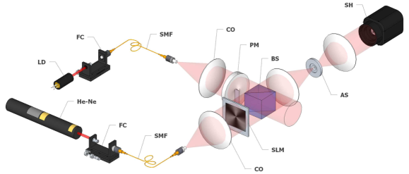
Figure 2: Experimental layout for preparing and detecting partially coherent vortex beams. Two independent laser sources, He-Ne at 633 nm (He-Ne) and a laser diode at 635 nm (LD), are coupled into single-mode fibers (SMF) by fiber couplers (FC). After collimation (CO) , they are transformed into vortex beams by two different techniques. The first beam, representing a coherent superposition of two vortex modes, is prepared by a digital hologram imprinted in a spatial light modulator (SLM). Unwanted diffraction orders are filtered by an aperture stop (AS), placed in a 4$f$ system. The second beam is modulated by a vortex phase mask (PM) and represents a single vortex mode with opposite phase respect to the first beam. Both beams are incoherently mixed in a beam splitter (BS) and finally detected in a SH sensor (SH).

To proceed further in this matter, we expand the signal as a finite superposition of a suitable spatially-unbounded computational basis (depending on the actual experiment, one should use plane waves, Laguerre-Gauss beams, etc). If that basis is labeled by $|{k}\rangle$ ($k=1,\ldots,d$, with $d$ being the dimension), the complex amplitudes are $\langle x|k\rangle=\psi_{k}(x)$. Therefore, the coherence matrix $\varrho$ and the measurement operators $\Pi_{ij}$ are given by $d\times d$ non-negative matrices. A convenient representation of $\Pi_{ij}$ can be obtained directly from Eq. (2), viz,

$$\left(\Pi_{ij}\right)_{mn}=\psi_{n,i}(\Delta p_{j})\,\psi_{m,i}^{\ast}(\Delta p_{j}),$$ (3)

where $\psi_{m,i}(x)$ is the complex amplitude at the CCD plane of the $i$th lens generated by the incident $m$th basis mode $\psi_{m}$.

This idea can be illustrated with the simple yet relevant example of square microlenses: $A(x)=\mathrm{rect}(x)$. We decompose the signal in a discrete set of plane waves $\psi_{k}(x)=\exp(-ip_{k}x)$, parametrized by the transverse momenta $p_{k}$. This is just the Fraunhofer diffraction on a slit, and the measurement matrix is

$$\left(\Pi_{ij}\right)_{mn}=\mathrm{sinc}(\Delta p_{j}+p_{m})\mathrm{sinc}(\Delta p_{j}+p_{n})e^{i(p_{m}-p_{n})\Delta x_{i}}\,.$$ (4)

The smallest possible search space consists of two plane waves (which is equivalent to a single-qubit tomography). By considering different pixels $j$ belonging to the same aperture $i$, linear combinations of only three out of the four Pauli matrices can be generated from Eq. (4). For example, a lens placed on the SH axis ($\Delta x_{i}=0$) fails to generate $\sigma_{y}$ and at least one more lens with a different $\Delta x_{i}$ needs to be added to the setup to make the tomography complete.

This argument can be easily extended: the larger the search space, the more microlenses must be used. In this example, the maximum number of independent measurements generated by the SH detection is $(2M+1)d-3M$, for $M$ lenses. A $d$-dimensional signal —a spatial qudit— can be characterized with about $M\sim d/2$ microlenses. This should be compared to the $d$ quadratures required for the homodyne reconstruction of a photonic qudit Leonhardt:1996bh ; Sych:2012qo .

Experiment. We have validated our method with vortex beams Molina:2007kn ; Torres:2011vn . Consider the one-parameter family of modes specified by the orbital angular momentum $\ell$, $V_{\ell}=\langle r,\varphi|\text{V}_{\ell}\rangle\propto\mathrm{e}^{\mathrm{i}\ell\varphi}$, where $(r,\varphi)$ are cylindrical coordinates. In our experiment, the partially coherent signal

$$\varrho_{\text{true}}=|V_{-3}-\textstyle{\frac{i}{2}}V_{-6}\rangle\langle V_{-3}-\textstyle{\frac{i}{2}}V_{-6}|+\frac{1}{2}|V_{3}\rangle\langle V_{3}|$$ (5)

was created; that is, modes $V_{-3}$ and $V_{-6}$ are coherently superposed, while $V_{3}$ is incoherently mixed. Figure 2 sketches the experimental layout used to generate (5). Imperfections of the setup and sensor noise makes the actual state to differ from the true state. Calibration and signal intensity scans are presented in Fig. 3.

The coherence matrix of the true state is expanded in the 7-dimensional space spanned by the modes $V_{\ell}$, with $\ell\in\{-9,-6,-3,0,+3,+6,+9\}$. The resulting matrix elements are plotted in Fig. 4.

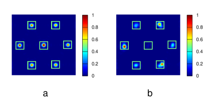
Figure 3: Experimental CCD signal. Rescaled 8-bit data corresponding to 7 microlenses placed in a hexagonal geometry, $81\times 81$-pixels region, is displayed in both panels. a) Data of the plane wave used for calibration; b) data of the partially coherent vortex beam in Eq. (5). Green squares enclose the data used for the reconstruction. The intensity from the central microlens vanishes due to the presence of a phase singularity.

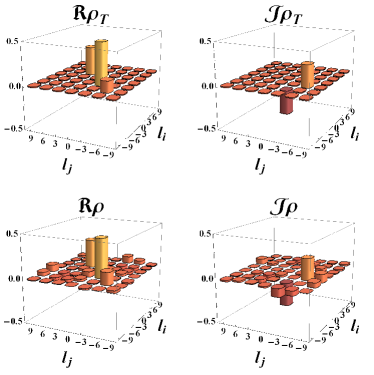
Figure 4: Vortex-beam coherence-matrix reconstruction. Real $\Re$ and imaginary $\Im$ parts of the coherence matrix for the true state $\varrho_{\mathrm{true}}$ (upper panel) and for the reconstructed $\varrho$ (lower panel). The reconstruction space is spanned by vortex modes with $\ell\in\{-9,-6,-3,0,+3,+6,+9\}$. The nonzero values of $\Im\varrho_{-6,-3}$ and $\Im\varrho_{-3,-6}$ describe coherences between the modes $|V_{-6}\rangle$ and $|V_{-3}\rangle$ and the phase shift $\pi$ between them. The very small values of $\varrho_{3,-6}$, $\varrho_{3,-3}$, $\varrho_{-6,3}$ and $\varrho_{-3,3}$ comes from the incoherent mixing of $|V_{3}\rangle$ and $|V_{-3}-\frac{i}{2}V_{-6}\rangle$. The fidelity of the reconstructed coherence matrix is $F=0.98$.

To reconstruct the state we use a maximum likelihood algorithm Hradil:2006il ; Rehacek:2009jl , whose results are summarized in Fig. 4. The main features of $\varrho_{\mathrm{true}}$ are nicely displayed, which is also confirmed by the high fidelity of the reconstructed state $F(\varrho_{\mathrm{true}},\varrho)=\mathop{\mathrm{Tr}}\nolimits[\sqrt{\sqrt{\varrho}\varrho_{\mathrm{true}}\sqrt{\varrho}}]=0.98$. The off-diagonal elements detect the coherence between modes, whereas the diagonal ones give the amplitude ratios between them. The reconstruction errors are mainly due to the difference between the true and the actually generated state.

To our best knowledge, this is the first experimental measurement of the coherence properties with a wavefront sensor. The procedure outperforms the standard SH operation, both in terms of dynamical range and resolution, even for fully coherent beams. For example, the high-order vortex beams with strongly helical wavefronts are very difficult to analyze with the standard wavefront sensors, while they pose no difficulty for our proposed approach.

The dynamical range and the resolution of the SH tomography are delimited by the choice of the search space $\{|k\rangle\}$ and can be quantified by the singular spectrum  Bogdanov:2011fk of the measurement matrix $\Pi_{ij}$. For the data in Fig. 4, the singular spectrum (which is the analog of the modulation transfer function in wave optics) is shown in Fig. 5. Depending on the threshold, around 20 out of the total of 49 modes spanning the space of $7\times 7$ coherence matrices can be discriminated. The modes outside this field of view are mainly those with significant intensity contributions out of the rectangular regions of the CCD sensor. Further improvements can be expected by exploiting the full CCD area and/or using a CCD camera with more resolution, at the expense of more computational resources for data post-processing.

3D Imaging. Once the feasibility of the SH tomography has been proven, we illustrate its utility with an experimental demonstration of 3D imaging (or digital propagation) of partially coherent fields.

As it is well known Goodman:2005qa , the knowledge of the transverse intensity distribution at an input plane is, in general, not sufficient for calculating the transverse profile at other output plane. Propagation requires the explicit form of the mutual coherence function $G_{\mathrm{in}}$ at the input to determine $I_{\mathrm{out}}$:

$$I_{\mathrm{out}}(\mathbf{x})=\iint_{-\infty}^{\infty}h(\mathbf{x},\mathbf{x}^{\prime})h^{\ast}(\mathbf{x},\mathbf{x}^{\prime\prime})\,G_{\mathrm{in}}(\mathbf{x}^{\prime},\mathbf{x}^{\prime\prime})d\mathbf{x}^{\prime}d\mathbf{x}^{\prime\prime}\,.$$ (6)

Here $\mathbf{x}^{\prime}$ ($\mathbf{x}^{\prime\prime}$) and $\mathbf{x}$ are the coordinates parametrizing the input and output planes, respectively, and $h(\mathbf{x},\mathbf{x}^{\prime})$ the response function accounting for propagation.

The dependence of the far-field intensity on the beam coherence properties is evidenced in Fig. 6 for coherent, partially coherent and incoherent superpositions of vortex beams.

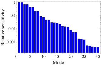
Figure 5: Dynamical range of the SH reconstruction. The singular spectrum $\{S_{kk}\}$ of the data in Fig. 4 (here, sorted and normalized to the largest singular value) quantifies the sensitivity of the tomography setup to the normal modes of the problem (see Methods). The relative strengths of the singular values correspond to the relative measuring accuracy of those modes. The dynamical range (or field of view) can be defined as the set of normal modes with singular values exceeding a given threshold.

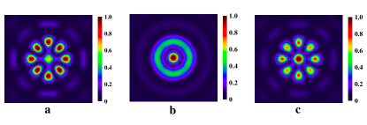
Figure 6: Influence of the spatial coherence on the far-field intensity distribution. We have considered different mixtures of the modes $|V_{4}\rangle$, $|V_{-4}\rangle$, and $|V_{0}\rangle$ and calculated the associated intensity distribution as a Fraunhofer diffraction pattern. (a) fully coherent superposition $|V_{4}+V_{-4}+0.4V_{0}\rangle\langle V_{4}+V_{-4}+0.4V_{0}|$; (b) incoherent mixture $|V_{4}\rangle\langle V_{4}|+|V_{-4}\rangle\langle V_{-4}|+0.4|V_{0}\rangle\langle V_{0}|$; and (c) partially coherent mixture $|V_{4}+V_{-4}\rangle\langle V_{4}+V_{-4}|+0.4|V_{0}\rangle\langle V_{0}|$.

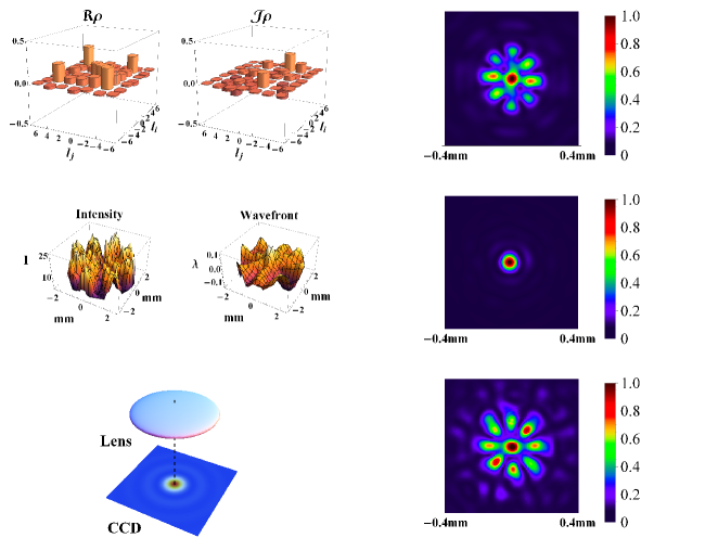
Figure 7: Digital 3D imaging. The prediction of the far-field intensity distribution is compared with a direct intensity measurement. The partially coherent vortex beam $|V_{4}+V_{-4}\rangle\langle V_{4}+V_{-4}|+k|V_{0}\rangle\langle V_{0}|$ was generated (with a beam diameter of 4.9 mm) with a fixed parameter $k$ (unknown prior to the reconstruction). . Upper, middle and lower pannels correspond to the SH tomography, standard SH measurement and direct intensity measurement, respectively. Upper left: Real and imaginary parts of the reconstructed $\varrho$ in the 7-dimensional space spanned by the vortices $V_{\ell}$ with $\ell\in\{-6,-4,-2,0,2,4,6\}$. Upper right: Calculated far-field intensity distribution $I_{\varrho}$ based on the reconstructed $\varrho$ propagated to the focal plane of the lens ($f=500$ mm). Middle left: Intensity distribution (in arbitrary units) and wavefront as measured by the standard SH sensor. Middle right: Calculated far-field intensity distribution $I_{\mathrm{std}}$ using the standard SH wavefront reconstruction and the transport of intensity equation included in the sensor (HASO™). Bottom left: Schematic picture of the direct intensity measurement at the lens focal plane. Bottom right: The result of the direct intensity measurement $I_{\mathrm{CCD}}$ at the focal plane with a CCD camera.

Once the coherence matrix is reconstructed, the forward/backward spatial propagation can be obtained using tools of diffraction theory and, consequently, the full 3D spatial intensity distribution can be computed. In particular, the intensity profile at the focal plane of an imaging system can be predicted from the SH measurements. This has been experimentally confirmed, as sketched in Fig. 7. We prepared the partially coherent superposition $|V_{4}+V_{-4}\rangle\langle V_{4}+V_{-4}|+k|V_{0}\rangle\langle V_{0}|$, and characterized by the SH tomography method. The reconstructed coherence function (upper left) was digitally propagated to the focal plane of a lens and the intensity distribution at this plane was calculated (upper right) and compared with the actual CCD scan in the same plane (lower right). Excellent agreement between the predicted and measured distributions was found.

We emphasize that the standard SH operation fails in this kind of application Schafer:2002rm . Indeed, we measured the intensity and wavefront of the target vortex superposition with a standard SH sensor (middle left) and propagated the measured intensity to the focal plane using the transport of intensity equation Teague:1983lq ; Roddier:1990ai (middle right). To quantify the result, we compute the normalized correlation coefficient [$C(I_{a},I_{b})=\sum_{i,j}I_{a}I_{b}/\sqrt{\sum_{i,j}I_{a}^{2}}\sqrt{\sum_{i,j}I_{b}^{2}}$] of the measured intensity with the prediction: the result, $C(I_{\mathrm{std}},I_{\mathrm{CCD}})=0.47$, confirms the inability of the standard SH to cope with the coherence properties of the signal. This has to be compared with the result for the SH tomography: $C(I_{\varrho},I_{\mathrm{CCD}})=0.89$, which supports its advantages.

Discussion

We have demonstrated a nontrivial coherence measurement with a SH sensor. This goes further the standard analysis and constitutes a substantial leap ahead that might trigger potential applications in many areas. Such a breakthrough would not have been possible without reinterpreting the SH operation as a simultaneous unsharp measurement of position and momentum. This immediately allows one to set a fundamental limit in the experimental accuracy Appleby:1998fp .

Moreover, although the SH has been the thread for our discussion, it is not difficult to extend the treatment to other wavefront sensors. For example, let us consider the recent results for temperature deviations of the cosmic microwave background Hinshaw:2009qq . The anisotropy is mapped as spots on the sphere, representing the distribution of directions of the incoming radiation. To get access to the position distribution, the detector has to be moved and, in principle, such a scanning brings information about the position and direction simultaneously: the position of the measured signal prior to detection is delimited by the scanning aperture, whereas the direction the signal comes from is revealed by the detector placed at the focal plane. When the aperture moves, it scans the field repeatedly at different positions. This could be an excellent chance to investigate the coherence properties of the relict radiation. To our best knowledge, this question has not been posed yet. Quantum tomography is especially germane for this task.

Finally, let us stress that classical estimation theory has been already applied to the raw SH image data, offering an improved accuracy, but at greater computational cost Cannon:1995qf ; Barrett:2007ao . However, the protocol used here can be implemented in a very easy, compact way, without any numerical burden.

Methods

Partially-coherent beam preparation. Two independent vortex beams were created in the setup of Fig. 2 with two laser sources of nearly the same wavelength: a He-Ne (633 nm) and a diode laser (635 nm). The output beams were spatialy filtered by coupling them into single-mode fibers. The power ratio between the modes was controlled by changing the coupling efficiency. The resulting modes were transformed into vortex beams by different methods.

The state $|V_{-3}-\textstyle{\frac{i}{2}}V_{-6}\rangle$ was realized using a digital hologram prepared with an amplitude spatial light modulator (OPTO SLM), with a resolution of 1024$\times$768 pixels. The hologram was then illuminated by a reference plane wave produced by placing the output of a single-mode fiber at the focal plane of a collimating lens. The diffraction spectrum involves several orders, of which only one contains useful information. To filter out the unwanted orders, a 4$f$ optical processor, with a 0.3 mm circular aperture stop placed at the rear focal plane of the second lens, was used. The resulting coherent vortex beam is then realized at the focal plane of the third lens.

The second beam $|V_{3}\rangle$ was obtained trough a plane-wave phase profile modulation by a special vortex phase mask (RPC Photonics). Finally, the field in Eq. (5) was prepared by mixing the two vortex modes in a beam splitter.

During the state preparation, special care was taken to reduce any deviation between the true and target states. This involved minimizing aberrations as well as imperfections of the spatial light modulator, resulting in distortions of the transmitted wavefront.

SH detection. The SH measurement involved a Flexible Optical array of 128 microlenses arranged in a hexagonal pattern. Each microlens has a focal length of 17.9 mm and a hexagonal aperture of 0.3 mm. The signal at the focal plane of the array is detected by a uEye CCD camera with a resolution of 640$\times$480 pixels, each pixel being 9.9 $\mu$m$\times$9.9 $\mu$m in size. Because of microlens array imperfections, CCD-microlens misalignment, and aberrations of the 4$f$ processor (aberrations of the collimating optics are negligible), calibration of the detector must be carried out. The holographic part of the setup provided this calibration wave. SH data from the calibration wave and the partially coherent beam are shown in Fig. 3. The beam axis position in the microlens array coordinates was adjusted with a Gaussian mode. The detection noise is mainly due to the background light, which is filtered out prior to reconstruction.

Reconstruction. The reconstruction was done in the $7$-dimensional space spanned by the $V_{\ell}$ modes with $\ell\in\{-9,-6,-3,0,+3,+6,+9\}$. All in all, $49$ real parameters had to be reconstructed. The data come from CCD areas belonging to 7 microlenses around the beam axis; each one of them comprise 11$\times$11 pixels, which means 847 data samples altogether. An iterative maximum-likelihood algorithm Hradil:2006il ; Rehacek:2009jl was applied to estimate the true coherence matrix of the signal.

Dynamical range and resolution. The errors of the SH tomography can be quantified by evaluating the covariances of the parameters of the reconstructed coherence matrix $\varrho$. In the absence of systematic errors, the Cramér-Rao lower bound Cramer:1946ye ; Rao:1973qo can be employed to that end. In practice, a simpler approach based on the singular spectrum analysis Bogdanov:2011fk works pretty well.

Let us decompose the $d\times d$ coherence matrix $\varrho$ ($d$ is just the dimension of the search space) and the measurement operators $\Pi_{ij}$ in an orthonormal matrix basis $\Gamma_{k}$ ($k=1,\ldots,d^{2}$) [$\mathop{\mathrm{Tr}}\nolimits(\Gamma_{k}\Gamma_{l})=\delta_{kl}$], namely

$$\varrho=\sum r_{k}\Gamma_{k},\qquad\Pi_{ij}=\sum_{k}p^{ij}_{k}\Gamma_{k},$$ (7)

so that the Born rule (2) can be recast as a system of linear equations

$$I_{ij}=\sum_{k}p^{ij}_{k}r_{k}\,.$$ (8)

Upon using a single index $\alpha$ to label all possible microlens/CCD-pixel combinations $\alpha\equiv\{i,j\}$, Eq. (8) can be concisely expressed in the matrix form

$$\mathbf{I}=\mathbf{P}\,\mathbf{r}\,,$$ (9)

where $\mathbf{I}$ is the vector of measured data, $\mathbf{r}$ is the vector of coherence-matrix parameters and $\mathrm{P}_{\alpha k}=p^{\alpha}_{k}$ is the tomography matrix.

Obviously, for ill-conditioned measurements, the reconstruction errors will be larger and vice versa. By applying a singular value decomposition to the measurement matrix $\mathbf{P}=\mathbf{U}\,\mathbf{S}\,\mathbf{V}^{\dagger}$, Eq. (9) takes the diagonal form

$$\mathbf{I}^{\prime}=\mathbf{S}\,\mathbf{r}^{\prime}\,,$$ (10)

where $\mathbf{r}^{\prime}=\mathbf{V}^{\dagger}\mathbf{r}$ and $\mathbf{I}^{\prime}=\mathbf{U}^{\dagger}\mathbf{I}$ are the normal modes of the problem and the corresponding transformed data, respectively. The singular values $\mathrm{S_{kk}}$ are the eigenvalues associated with the normal modes, so the relative sensitivity of the tomography to different normal modes is given by the relative sizes of the corresponding singular values. With the help of Eqs. (9) and (10), the errors are readily propagated form the detection $\mathbf{I}$ to the reconstruction $\mathbf{r}$.

Drawing an analogy between Eq. (10) and the filtering by a linear spatially invariant system, the singular spectrum $\mathrm{S}_{kk}$ and the sum of the singular values $\sum_{k}\mathrm{S}_{kk}$ are the discrete analogs of the modulation transfer function and the maximum of the point spread function, respectively. Hence we define the dynamical range (or field of view) of the SH tomography as the set of normal modes with singular values exceeding a given threshold. The sum of the singular values then describes the overall performance of the SH tomography setup. When some of the singular values are zero, the tomography is not informationally complete and the search space must be readjusted.

Far-field intensity. In the experiment on 3D imaging, the partially coherent vortex beam $|V_{4}+V_{-4}\rangle\langle V_{4}+V_{-4}|+k|V_{0}\rangle\langle V_{0}|$ was generated, where $k$ was a parameter governing the degree of spatial coherence. To this end, a coherent mixture $|V_{4}+V_{-4}\rangle\langle V_{4}+V_{-4}|$ was realized by the digital-holography part of the setup, whereas the zero-order vortex beam $|V_{0}\rangle$ was prepared by removing the spiral phase mask. The output diameter of the beam was set to 4.9 mm.

The measurement was done in three steps. First, the SH sensor (see Fig. 2) was replaced by a lens of 500 mm focal length and the far-field intensity was detected at its rear focal plane with a CCD camera (Olympus F-View II, 1376$\times$1032 pixels, 6.45 $\mu$m$\times$6.45 $\mu$m each). Second, the same vortex superposition was subject to the SH tomography using the SH sensor (Flexible Optical) and the reconstruction of the coherence matrix in the 7-dimensional subspace spaned by the vortices $V_{\ell}$ with $\ell\in\{-6,-4,-2,0,+2,+4,+6\}$. Once $\varrho$ is reconstructed, the far-field intensity was computed using Eq. (6), where the focusing is described by the Fraunhofer diffraction response function. The predicted intensity was found to be in an excellent agreement with the direct sampling by the Olympus CCD camera. Finally, the Flexible Optical SH sensor was replaced by a HASO3 SH detector. The intensity and wavefront of the prepared vortex beam was measured and the far-field intensity was computed by resorting to the transport of intensity performed by the HASO software. Resampling was done to match the resolution of the HASO output to the resolution of the Olympus CCD camera.

Acknowledgments

This work was supported by the Technology Agency of the Czech Republic (Grant TE01020229), the Czech Ministry of Industry and Trade (Grant FR-TI1/364), the IGA Projects of the Palacký University (Grants PRF  2012  005 and PRF  2013  019) and the Spanish MINECO (Grant FIS2011-26786).

Contributions

The experiment was conceived by J.R., Z.H. and L.L.S.S and carried out by B.S. The numerical reconstruction was performed by B.S., whereas J. R. and L. M. provided theoretical analysis. Z.H. and J.R. supervised the project. The theoretical part of manuscript was written by L.L.S.S. and J.R. and the experimental part by B. S. and L.L.S.S., with input and discussions from all other authors.

References

- (1) D. Malacara, ed., Optical Shop Testing (Wiley, Hoboken, 2007), 3rd ed.
- (2) G.-M. Dai, Wavefront Optics for Vision Correction (SPIE Press, Bellingham, 2008).
- (3) J. Ares, T. Mancebo, and S. Bar·, “Position and displacement sensing with Shack-Hartmann wave-front sensors,” Appl. Opt. 39, 1511–1520 (2000).
- (4) O. Katz, E. Small, Y. Bromberg, and Y. Silberberg, “Focusing and compression of ultrashort pulses through scattering media,” Nat. Photon. 5, 372–377 (2011).
- (5) D. J. McCabe, A. Tajalli, D. R. Austin, P. Bondareff, I. A. Walmsley, S. Gigan, and B. Chatel, “Spatio-temporal focusing of an ultrafast pulse through a multiply scattering medium,” Nat. Commun. 2, 447 (2011).
- (6) A. P. Mosk, A. Lagendijk, G. Lerosey, and M. Fink, “Controlling waves in space and time for imaging and focusing in complex media,” Nat. Photon. 6, 283–292 (2012).
- (7) R. K. Tyson, Principles of Adaptive Optics (CRC Press, Boca Raton, 2011), 3rd ed.
- (8) J. M. Geary, Introduction to Wavefront Sensors (SPIE Press, Bellingham, 1995).
- (9) D. R. Luke, J. V. Burke, and R. G. Lyon, “Optical wavefront reconstruction: Theory and numerical methods,” SIAM Rev. 44, 169—224 (2002).
- (10) H. I. Campbell and A. H. Greenaway, “Wavefront sensing: From historical roots to the state-of-the-art.” EAS Publications 22, 165–185 (2006).
- (11) B. C. Platt and R. S. Shack, “History and principles of Shack-Hartmann wavefront sensing,” J. Refract. Surg. 17, S573–S577 (2001).
- (12) J. Primot, “Theoretical description of Shack-Hartmann wave-front sensor,” Opt. Commun. 222, 81–92 (2003).
- (13) L. Mandel and E. Wolf, Optical Coherence and Quantum Optics (Cambridge University Press, Cambridge, 1995).
- (14) Z. Hradil, J. Řeháček, and L. L. Sánchez-Soto, “Quantum reconstruction of the mutual coherence function,” Phys. Rev. Lett. 105, 010401 (2010).
- (15) M. G. A. Paris and J. Řeháček, eds., Quantum State Estimation, vol. 649 of Lect. Not. Phys. (Springer, Berlin, 2004).
- (16) J. W. Goodman, Introduction to Fourier Optics (Roberts, Greenwood Village, 2005), 3rd ed.
- (17) E. Arthurs and J. L. J. Kelly, “On the simultaneous measurement of a pair of conjugate observables,” Bell Syst. Tech. J. 44, 725–729 (1965).
- (18) S. Stenholm, “Simultaneous measurement of conjugate variables,” Ann. Phys. 218, 197–198 (1992).
- (19) M. G. Raymer, “Uncertainty principle for joint measurement of noncommuting variables,” Am. J. Phys. 62, 986–993 (1994).
- (20) K. Husimi, “Some formal properties of the density matrix,” Proc. Phys. Math. Soc. Jpn. 22, 264–314 (1940).
- (21) A. I. Lvovsky and M. G. Raymer, “Continuous-variable optical quantum-state tomography,” Rev. Mod. Phys. 81, 299–322 (2009).
- (22) P. Busch and P. Lahti, “The determination of the past and the future of a physical system in quantum mechanics,” Found. Phys. 19, 633–678 (1989).
- (23) U. Leonhardt and M. Munroe, “Number of phases required to determine a quantum state in optical homodyne tomography,” Phys. Rev. A 54, 3682–3684 (1996).
- (24) D. Sych, J. Řeháček, Z. Hradil, G. Leuchs, and L. L. Sánchez-Soto, “Informational completeness of continuous-variable measurements,” Phys. Rev. A 86, 052123 (2012).
- (25) G. Molina-Terriza, J. P. Torres, and L. Torner, “Twisted photons,” Nat. Phys. 3, 305–310 (2007).
- (26) J. Torres and L. Torner, eds., Twisted Photons: Applications of Light with Orbital Angular Momentum. (Wiley-VCH, Weinheim, 2011).
- (27) Z. Hradil, D. Mogilevtsev, and J. Řeháček, “Biased tomography schemes: An objective approach,” Phys. Rev. Lett. 96, 230401 (2006).
- (28) J. Řeháček, Z. Hradil, Z. Bouchal, R. Čelechovský, I. Rigas, and L. L. Sánchez-Soto, “Full tomography from compatible measurements,” Phys. Rev. Lett. 103, 250402 (2009).
- (29) Y. I. Bogdanov, G. Brida, I. D. Bukeev, M. Genovese, K. S. Kravtsov, S. P. Kulik, E. V. Moreva, A. A. Soloviev, and A. P. Shurupov, “Statistical estimation of the quality of quantum-tomography protocols,” Phys. Rev. A 84, 042108 (2011).
- (30) B. Schäfer and K. Mann, “Determination of beam parameters and coherence properties of laser radiation by use of an extended Hartmann–Shack wave-front sensor,” Appl. Opt. 41, 2809–2817 (2002).
- (31) M. R. Teague, “Deterministic phase retrieval: a Green’s function solution,” J. Opt. Soc. Am. A 73, 1434–1441 (1983).
- (32) F. Roddier, “Wavefront sensing and the irradiance transport equation,” Appl. Opt. 29, 1402–1403 (1990).
- (33) D. M. Appleby, “Concept of experimental accuracy and simultaneous measurements of position and momentum,” Int. J. Theor. Phys. 37, 1491–1509 (1998).
- (34) G. Hinshaw, J. L. Weiland, R. S. Hill, N. Odegard, D. Larson, C. L. Bennett, J. Dunkley, B. Gold, M. R. Greason, N. Jarosik, E. Komatsu, M. R. Nolta, L. Page, D. N. Spergel, E. Wollack, M. Halpern, A. Kogut, M. Limon, S. S. Meyer, G. S. Tucker, and E. L. Wright, “Five-year Wilkinson microwave anisotropy probe observations: Data processing, sky maps, and basic results,” Astrophys. J. Suppl Ser. 180, 225–245 (2009).
- (35) R. C. Cannon, “Global wave-front reconstruction using Shack-Hartmann sensors,” J. Opt. Soc. Am. A 12, 2031–2039 (1995).
- (36) H. H. Barrett, C. Dainty, and D. Lara, “Maximum-likelihood methods in wavefront sensing: stochastic models and likelihood functions,” J. Opt. Soc. Am. A 24, 391–414 (2007).
- (37) H. Cramér, Mathematical Methods of Statistics (Princeton University, Princeton, 1946).
- (38) C. R. Rao, Linear Statistical Inference and Its Applications (Wiley, New York, 1973).