Modeling of Degradation Processes in Historical Mortars

Abstract

The aim of presented paper is modeling of degradation processes in historical mortars exposed to moisture impact during freezing. Internal damage caused by ice crystallization in pores is one of the most important factors limiting the service life of historical structures. Coupling the transport processes with the mechanical part will allow us to address the impact of moisture on the durability, strength and stiffness of mortars. This should be accomplished with the help of a complex thermo-hygro-mechanical model representing one of the prime objectives of this work. The proposed formulation is based on the extension of the classical poroelasticity models with the damage mechanics. An example of two-dimensional moisture transport in the environment with temperature below freezing point is presented to support the theoretical derivations.

^∗Department of Mechanics, Faculty of Civil Engineering

Czech Technical University in Prague

Thákurova 7, 166 29 Prague, Czech Republic

Dedicated to Professor Zdeněk Bittnar in ocassion of his 70th birthday.

Keywords: Coupled heat and moisture transport, ice crystallization process, damage, mortar.

Nomenclature

$a$	water absorption coefficient, $\mathrm{[kgm^{-2}s^{-0.5}]}$
$\mathchoice{\displaystyle\boldsymbol{b}}{\textstyle\boldsymbol{b}}{\scriptstyle\boldsymbol{b}}{\scriptscriptstyle\boldsymbol{b}}$	body force, $\mathrm{[Nm^{-3}]}$
$b$	Biot’s coefficient, $\mathrm{[-]}$
$b_{\mathrm{tcs}}$	thermal conductivity supplement, $\mathrm{[-]}$
$b_{\varphi}$	approximation factor, $\mathrm{[-]}$
$\mathchoice{\displaystyle\mathbf{C}}{\textstyle\mathbf{C}}{\scriptstyle\mathbf{C}}{\scriptscriptstyle\mathbf{C}}$	discretized capacity matrix
$c_{\mathrm{i}}$	specific heat capacity of ice, $\mathrm{[Jkg^{-1}K^{-1}]}$
$c_{\mathrm{s}}$	specific heat capacity of solid matrix, $\mathrm{[Jkg^{-1}K^{-1}]}$
$c_{\mathrm{l}}$	specific heat capacity of liquid water, $\mathrm{[Jkg^{-1}K^{-1}]}$
$\mathchoice{\displaystyle\mathbf{D}}{\textstyle\mathbf{D}}{\scriptstyle\mathbf{D}}{\scriptscriptstyle\mathbf{D}}_{e}$	elastic stiffness matrix, $\mathrm{[Pa]}$
$D_{\mathrm{l}}$	capillary transport coefficient, $\mathrm{[m^{2}s^{-1}]}$
$D_{\varphi}$	liquid conduction coefficient, $\mathrm{[kgm^{-1}s^{-1}]}$
$d_{w}$	damage parameter, $\mathrm{[-]}$
$E$	Young’s modulus, $\mathrm{[Pa]}$
$\mathchoice{\displaystyle\boldsymbol{F}}{\textstyle\boldsymbol{F}}{\scriptstyle\boldsymbol{F}}{\scriptscriptstyle\boldsymbol{F}}$	prescribed fluxes
$f_{t}$	tensile strength, $\mathrm{[Pa]}$
$H$	total enthalpy of porous material, $\mathrm{[Jm^{-3}]}$
$h_{\mathrm{i}}$	specific melting enthalpy of ice, $\mathrm{[Jkg^{-1}]}$
$h_{\mathrm{v}}$	latent heat of phase exchange, $\mathrm{[Jkg^{-1}]}$
$\mathchoice{\displaystyle\mathbf{K}}{\textstyle\mathbf{K}}{\scriptstyle\mathbf{K}}{\scriptscriptstyle\mathbf{K}}$	discretized conductivity matrix
$K$	bulk modulus of porous material, $\mathrm{[Pa]}$
$K_{\mathrm{s}}$	bulk modulus of solid matrix, $\mathrm{[Pa]}$
$l_{\mathrm{intl}}$	internal length, $\mathrm{[m]}$
$M_{w}$	molar mass of water, $\mathrm{[kgmol^{-1}]}$
$\mathchoice{\displaystyle\boldsymbol{n}}{\textstyle\boldsymbol{n}}{\scriptstyle\boldsymbol{n}}{\scriptscriptstyle\boldsymbol{n}}$	unit normal vector, $\mathrm{[-]}$

$n$	total porosity, $\mathrm{[-]}$
$p_{\mathrm{a}}$	atmospheric pressure, $\mathrm{[Pa]}$
$p_{\mathrm{l}}$	liquid pressure, $\mathrm{[Pa]}$
$p_{\mathrm{p}}$	average pore pressure, $\mathrm{[Pa]}$
$p_{\mathrm{sat}}$	saturation vapor pressure, $\mathrm{[Pa]}$
$\mathchoice{\displaystyle\boldsymbol{q}}{\textstyle\boldsymbol{q}}{\scriptstyle\boldsymbol{q}}{\scriptscriptstyle\boldsymbol{q}}_{\mathrm{h}}$	heat flux, $\mathrm{[Wm^{-2}]}$
$\mathchoice{\displaystyle\boldsymbol{q}}{\textstyle\boldsymbol{q}}{\scriptstyle\boldsymbol{q}}{\scriptscriptstyle\boldsymbol{q}}_{\mathrm{l}}$	liquid transport flux, $\mathrm{[kgm^{-2}s^{-1}]}$
$\mathchoice{\displaystyle\boldsymbol{q}}{\textstyle\boldsymbol{q}}{\scriptstyle\boldsymbol{q}}{\scriptscriptstyle\boldsymbol{q}}_{\mathrm{v}}$	water vapor flux, $\mathrm{[kgm^{-2}s^{-1}]}$
$R$	gas constant, $\mathrm{[Jmol^{-1}K^{-1}]}$
$r$	pore radius, $\mathrm{[m]}$
$\mathchoice{\displaystyle\boldsymbol{r}}{\textstyle\boldsymbol{r}}{\scriptstyle\boldsymbol{r}}{\scriptscriptstyle\boldsymbol{r}}$	nodal values
$r_{\mathrm{ar}}$	layer of adsorbed water, $\mathrm{[m]}$
$r_{\mathrm{cr}}$	critical pore radius, $\mathrm{[m]}$
$r_{\mathrm{ir}}$	curvature radius of ice crystal, $\mathrm{[m]}$
$S_{h}$	heat source, $\mathrm{[Wm^{-3}]}$
$S_{w}$	moisture source, $\mathrm{[kgm^{-3}s^{-1}]}$
$t$	time, $\mathrm{[s]}$
$\mathchoice{\displaystyle\boldsymbol{u}}{\textstyle\boldsymbol{u}}{\scriptstyle\boldsymbol{u}}{\scriptscriptstyle\boldsymbol{u}}$	displacement vector, $\mathrm{[m]}$
$w$	total water content, $\mathrm{[kgm^{-3}]}$
$w_{\mathrm{80}}$	water content at $0.8\,\mathrm{[-]}$ relative humidity, $\mathrm{[kgm^{-3}]}$
$w_{\mathrm{i}}$	content of ice, $\mathrm{[kgm^{-3}]}$
$w_{f}$	free water saturation, $\mathrm{[kgm^{-3}]}$
$\alpha$	thermal expansion coefficient, $\mathrm{[K^{-1}]}$
$\alpha_{\mathrm{h}}$	heat transfer coefficient, $\mathrm{[Wm^{-2}K^{-1}]}$
$\alpha_{\mathrm{swr}}$	short wave absorption coefficient, $\mathrm{[-]}$
$\beta_{\mathrm{v}}$	water vapor transfer coefficient, $\mathrm{[kgm^{-2}s^{-1}Pa^{-1}]}$
$\Gamma$	boundary
$\gamma$	generalized midpoint integration parameter, $\mathrm{[-]}$
$\gamma_{\mathrm{li}}$	liquid/ice surface tension, $\mathrm{[Nm^{-1}]}$
$\Delta s_{\mathrm{m}}$	melting entropy, $\mathrm{[PaK^{-1}]}$
$\delta$	vapor diffusion coefficient in air, $\mathrm{[kgm^{-1}s^{-1}Pa^{-1}]}$
$\delta_{\mathrm{v}}$	water vapor permeability of porous material, $\mathrm{[kgm^{-1}s^{-1}Pa^{-1}]}$
$\varepsilon_{\mathrm{0}}$	equivalent strain at elastic limit, $\mathrm{[-]}$
$\varepsilon_{\mathrm{eq}}$	equivalent strain, $\mathrm{[-]}$
$\varepsilon_{f}$	equivalent strain at critical crack opening, $\mathrm{[-]}$
$\theta$	temperature, $\mathrm{[^{\circ}C]}$
$\lambda$	thermal conductivity of moist porous material, $\mathrm{[Wm^{-1}K^{-1}]}$
$\lambda_{\mathrm{0}}$	thermal conductivity of dry porous material, $\mathrm{[Wm^{-1}K^{-1}]}$

$\mu$	water vapor diffusion resistance factor, $\mathrm{[-]}$
$\nu$	Poisson’s ratio, $\mathrm{[-]}$
$\rho_{\mathrm{s}}$	bulk density, $\mathrm{[kgm^{-3}]}$
$\mathchoice{\displaystyle\boldsymbol{\sigma}}{\textstyle\boldsymbol{\sigma}}{\scriptstyle\boldsymbol{\sigma}}{\scriptscriptstyle\boldsymbol{\sigma}}$	total stress, $\mathrm{[Pa]}$
$\mathchoice{\displaystyle\boldsymbol{\sigma}}{\textstyle\boldsymbol{\sigma}}{\scriptstyle\boldsymbol{\sigma}}{\scriptscriptstyle\boldsymbol{\sigma}}^{\prime}$	effective stress, $\mathrm{[Pa]}$
$\varphi$	relative humidity, $\mathrm{[-]}$
$\chi$	local pressure on the frozen pore walls, $\mathrm{[Pa]}$
$\psi$	cumulative volume of pores, $\mathrm{[-]}$
$\Omega$	domain
Subscripts
ext	exterior
i	ice
in	initial
int	interior
l	liquid water
p	pore
r	radius
s	solid
v	water vapor

1 Introduction

Understanding the hydro-thermo-mechanical behavior of building materials exposed to weather conditions is the first step toward avoiding deterioration of structures in general and historical ones in particular, as high moisture content in building material and its phase changes are often a cause of internal damage. Because of variable climatic conditions, the moisture gradients induce mechanical stresses in the porous material. These stresses mostly develop due to the growth of ice crystals through the pore structure. Therefore, there is a strong need for investigating the influence of moisture on the mechanical material behavior, which leads to numerical and experimental coupling of mechanical and thermo-hygro phenomena.

In the literature, the above described problem is addressed from several perspectives. The first group of publications is focused on the description of the coupled heat and moisture transport reflecting the moisture migration under the conditions of the ice crystal formation in the pores, $2$-D and $3$-D aspects and different moisture/heat sources, such as wind driven rain, solar short and long wave radiation etc., see  [8, 10, 25]. An extensive overview of various transport models is available in [12, 26]. While models for transport processes have been developed during several decades, the theory of ice crystallization in the pores has emerged only recently,  [19, 20, 22]. The authors established relations between physical state of porous system and pore pressures. The physical conditions of ice formation process are described by thermodynamic balance equation between ice, liquid water and solid matrix. Finally, the mechanical response of porous media subjected to the frost action was studied by several authors  [4, 27, 28]. On the one hand, the poroelasticity formulation based on Biot’s continuum model was adopted. It is an efficient method for elastic modeling of porous system, which is subjected to the pressure of the fluid. On the other hand, a novel micromechanics approach was introduced to analyze the creation of micro-cracks in the microstructure during freezing process  [9, 13]. These results predict effective mechanical and transport properties at microscopic level and can be utilized as an input for multi-scale analysis of porous media.

As a preamble, our goal is to quantify the internal damage caused by the ice crystallization pressure in historical mortars. In particular, a critical point in a restoration works is frequent applications of lime mortars for preserving compatibility with the historical materials. However, lime mortars are very porous, their mechanical strength and durability are mostly very low  [17, 21], thus the development of a lime mortar with improved internal hydrophobicity and associated improved resistance against damage due to the effects of ice crystallization is inevitable. To address this issue with respect to its complexity, an analysis combining both experimental work and numerical simulations has to be done. Nevertheless, the numerical methodology developed within this work can be utilized to simulate the response of any porous material subjected to the frost action.

A theoretical formulation of the problem is presented in Section 2, followed by numerical calculations in Section 3. Section 3.1 then investigates the influence of pore size distribution on the evolution of damage parameter. The essential findings are summarized in Section 4.

2 Material model

The problem of porous system subjected to ice crystallization can be divided into three physical phenomena - heat and moisture transport, ice formation process and evolution of damage caused by pore pressure. Using the thermodynamics, poromechanics and damage mechanics, we propose here the concept of multi-phase constitutive model based on the assumption of the uncoupled system in the sense of numerical analysis, see Fig. 1. These models are characterized by combining different physical or mechanical models (in space and time) in order to accurately describe structural response of deteriorating infrastructure over time. The general framework of the proposed model was primarily inspired by the work published in [1, 2, 4, 6, 10, 19, 27, 28].

In the presented work, the porous material is treated as multi-phase medium consisting of solid matrix, liquid water, water vapor and ice. The mathematical formulation consists of three governing equations representing the conservations of energy Eq. (4), mass Eq. (5) and linear momentum Eq. (36). The chosen primary unknowns are temperature $\theta\,\mathrm{[^{\circ}C]}$, moisture $\varphi\,\mathrm{[-]}$ and displacement of solid matrix $\mathchoice{\displaystyle\boldsymbol{u}}{\textstyle\boldsymbol{u}}{\scriptstyle\boldsymbol{u}}{\scriptscriptstyle\boldsymbol{u}}\,\mathrm{[m]}$.

Figure 1: Algorithmic framework of proposed model

The present section derives the governing equations of the analytical model. After theoretical formulation, a proper numerical time and space integration scheme is introduced to convert the proposed governing equations into a fully discrete form. Some details on the numerical implementation are also available in [11, 24].

2.1 Transport model

We use the diffusion model by Künzel, see [10], which is based on Krischer’s concept [26]. Künzel neglected the liquid water and water vapor convection driven by gravity and total pressure as well as enthalpy changes due to liquid flow and choose relative humidity $\varphi$ as the only moisture driving force. The water vapor diffusion is then described by Fick’s law written as

$$\mathchoice{\displaystyle\boldsymbol{q}}{\textstyle\boldsymbol{q}}{\scriptstyle\boldsymbol{q}}{\scriptscriptstyle\boldsymbol{q}}_{\mathrm{v}}=-\delta_{\mathrm{v}}\mathchoice{\displaystyle\boldsymbol{\nabla}}{\textstyle\boldsymbol{\nabla}}{\scriptstyle\boldsymbol{\nabla}}{\scriptscriptstyle\boldsymbol{\nabla}}\left(\varphi p_{\mathrm{sat}}\right),$$ (1)

where $\mathchoice{\displaystyle\boldsymbol{q}}{\textstyle\boldsymbol{q}}{\scriptstyle\boldsymbol{q}}{\scriptscriptstyle\boldsymbol{q}}_{\mathrm{v}}\,\mathrm{[kgm^{-2}s^{-1}]}$ is the water vapor flux, $\delta_{\mathrm{v}}\,\mathrm{[kgm^{-1}s^{-1}Pa^{-1}]}$ is the water vapor permeability of a porous material and $p_{\mathrm{sat}}=p_{\mathrm{sat}}(\theta)\,\mathrm{[Pa]}$ is the saturation water vapor pressure being exponentially dependent on temperature. The transport of liquid water is assumed in the form of surface diffusion in an absorbed layer and capillary flow typically represented by Kelvin’s law

$$\mathchoice{\displaystyle\boldsymbol{q}}{\textstyle\boldsymbol{q}}{\scriptstyle\boldsymbol{q}}{\scriptscriptstyle\boldsymbol{q}}_{\mathrm{l}}=-D_{\varphi}\mathchoice{\displaystyle\boldsymbol{\nabla}}{\textstyle\boldsymbol{\nabla}}{\scriptstyle\boldsymbol{\nabla}}{\scriptscriptstyle\boldsymbol{\nabla}}\varphi,$$ (2)

where $\mathchoice{\displaystyle\boldsymbol{q}}{\textstyle\boldsymbol{q}}{\scriptstyle\boldsymbol{q}}{\scriptscriptstyle\boldsymbol{q}}_{\mathrm{l}}\,\mathrm{[kgm^{-2}s^{-1}]}$ is the flux of liquid water, $D_{\varphi}=D_{\mathrm{l}}\,(\mathrm{d}w/\mathrm{d}\varphi)\,\mathrm{[kgm^{-1}s^{-1}]}$ is the liquid conductivity and $D_{\mathrm{l}}\,\mathrm{[m^{2}s^{-1}]}$ is the capillary transport coefficient, $\mathrm{d}w/\mathrm{d}\varphi$ is the derivative of water retention function. The Fourier law is then used to express the heat flux $\mathchoice{\displaystyle\boldsymbol{q}}{\textstyle\boldsymbol{q}}{\scriptstyle\boldsymbol{q}}{\scriptscriptstyle\boldsymbol{q}}_{\mathrm{h}}\,\mathrm{[Wm^{-2}]}$ as

$$\mathchoice{\displaystyle\boldsymbol{q}}{\textstyle\boldsymbol{q}}{\scriptstyle\boldsymbol{q}}{\scriptscriptstyle\boldsymbol{q}}_{\mathrm{h}}=-\lambda\mathchoice{\displaystyle\boldsymbol{\nabla}}{\textstyle\boldsymbol{\nabla}}{\scriptstyle\boldsymbol{\nabla}}{\scriptscriptstyle\boldsymbol{\nabla}}\theta,$$ (3)

where $\lambda\,\mathrm{[Wm^{-1}K^{-1}]}$ is the thermal conductivity and $\theta\,\mathrm{[^{\circ}C]}$ is the local temperature. Introducing the above constitutive equations into energy and mass conservation equations we finally get resulting set of differential equations for the description of heat and moisture transfer expressed in terms of temperature and relative humidity as

• the energy balance equation

  $$\frac{\partial H}{\partial\theta}\frac{\partial\theta}{\partial t}=\mathchoice{\displaystyle\boldsymbol{\nabla}}{\textstyle\boldsymbol{\nabla}}{\scriptstyle\boldsymbol{\nabla}}{\scriptscriptstyle\boldsymbol{\nabla}}\cdot[\lambda\mathchoice{\displaystyle\boldsymbol{\nabla}}{\textstyle\boldsymbol{\nabla}}{\scriptstyle\boldsymbol{\nabla}}{\scriptscriptstyle\boldsymbol{\nabla}}\theta]+h_{\mathrm{v}}\mathchoice{\displaystyle\boldsymbol{\nabla}}{\textstyle\boldsymbol{\nabla}}{\scriptstyle\boldsymbol{\nabla}}{\scriptscriptstyle\boldsymbol{\nabla}}\cdot[\delta_{\mathrm{v}}\mathchoice{\displaystyle\boldsymbol{\nabla}}{\textstyle\boldsymbol{\nabla}}{\scriptstyle\boldsymbol{\nabla}}{\scriptscriptstyle\boldsymbol{\nabla}}\{\varphi p_{\mathrm{sat}}(\theta)\}],$$ (4)

• the conservation of mass equation

  $$\frac{\mathrm{d}w}{\mathrm{d}\varphi}\frac{\partial\varphi}{\partial t}=\mathchoice{\displaystyle\boldsymbol{\nabla}}{\textstyle\boldsymbol{\nabla}}{\scriptstyle\boldsymbol{\nabla}}{\scriptscriptstyle\boldsymbol{\nabla}}\cdot[D_{\varphi}\mathchoice{\displaystyle\boldsymbol{\nabla}}{\textstyle\boldsymbol{\nabla}}{\scriptstyle\boldsymbol{\nabla}}{\scriptscriptstyle\boldsymbol{\nabla}}\varphi]+\mathchoice{\displaystyle\boldsymbol{\nabla}}{\textstyle\boldsymbol{\nabla}}{\scriptstyle\boldsymbol{\nabla}}{\scriptscriptstyle\boldsymbol{\nabla}}\cdot[\delta_{\mathrm{v}}\mathchoice{\displaystyle\boldsymbol{\nabla}}{\textstyle\boldsymbol{\nabla}}{\scriptstyle\boldsymbol{\nabla}}{\scriptscriptstyle\boldsymbol{\nabla}}\{\varphi p_{\mathrm{sat}}(\theta)\}]\,,$$ (5)

The transport coefficients defining the material behavior are nonlinear functions of the temperature, moisture and material properties. We briefly recall their particular expressions [10]:

• $w$ - total water content $\mathrm{[kgm^{-3}]}$,

  $$w=w_{f}\frac{(b_{\varphi}-1)\varphi}{b_{\varphi}-\varphi},$$ (6)

  where $w_{f}\,\mathrm{[kgm^{-3}]}$ is the free water saturation and $b_{\varphi}\,\mathrm{[-]}$ is the approximation factor, which must always be greater than one. It can be determined from the equilibrium water content ($w_{80}$) at $0.8$ [-] relative humidity by substituting the corresponding numerical values in Eq. (6). Fig. 2(a) shows an example of variation of water content as a function of relative humidity.

• $\delta_{\mathrm{v}}$ - water vapor permeability $\mathrm{[kgm^{-1}s^{-1}Pa^{-1}]}$,

  $$\delta_{\mathrm{v}}=\frac{\delta}{\mu},$$ (7)

  where $\mu\,\mathrm{[-]}$ is the water vapor diffusion resistance factor and $\delta\,\mathrm{[kgm^{-1}s^{-1}Pa^{-1}]}$ is the vapor diffusion coefficient in air given by

  $$\delta=\frac{2.306\cdot{}10^{-5}\,p_{\mathrm{a}}}{R_{\mathrm{v}}\,(\theta+273.15)\,p}\left(\frac{\theta+273.15}{273.15}\right)^{1.81},$$ (8)

  with $p$ set equal to atmospheric pressure $p_{a}=101325$ [Pa] and $R_{\mathrm{v}}$ = $R$/$M_{w}=461.5$ [$\mathrm{Jkg^{-1}K^{-1}}$]; $R$ is the gas constant ($8314.41$ [Jmol^-1K^-1]) and $M_{w}$ is the molar mass of water ($18.01528$ [kgmol^-1]). An example of variation of water vapor permeability as a function of temperature is seen in Fig. 2(b).

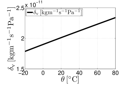
  (a)	(b)
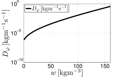
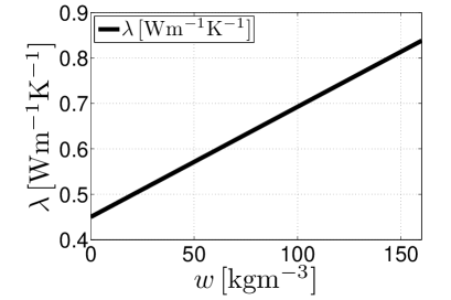
  (c)	(d)

  Figure 2: (a) Variation of water content as a function of relative humidity, (b) variation of water vapor permeability as a function temperature, (c) variation of liquid conductivity as a function of water content, (d) variation of thermal conductivity as a function of water content

• $D_{\varphi}$ - liquid conduction coefficient $\mathrm{[kgm^{-1}s^{-1}]}$,

  $$D_{\varphi}=D_{\mathrm{l}}\frac{\mathrm{d}w}{\mathrm{d}\varphi},$$ (9)

  where $D_{\mathrm{l}}\,\mathrm{[m^{2}s^{-1}]}$ is the capillary transport coefficient given by

  $$D_{\mathrm{l}}=3.8\left(\frac{a}{w_{f}}\right)^{2}\cdot{}10^{3w/(w_{f}-1)},$$ (10)

  An example of variation of liquid conductivity $D_{\varphi}\,\mathrm{[kgm^{-1}s^{-1}]}$ as a function of water content is plotted in Fig. 2(c).

• $\lambda$ - thermal conductivity $\mathrm{[Wm^{-1}K^{-1}]}$,

  $$\lambda=\lambda_{0}\left(1+\frac{b_{\mathrm{tcs}}w}{\rho_{\mathrm{s}}}\right),$$ (11)

  where $\lambda_{0}\,\mathrm{[Wm^{-1}K^{-1}]}$ is the thermal conductivity of dry building material, $\rho_{\mathrm{s}}\,\mathrm{[kgm^{-3}]}$ is the bulk density and $b_{\mathrm{tcs}}\,\mathrm{[-]}$ is the thermal conductivity supplement. An example of variation of thermal conductivity as a function of water content is shown in Fig. 2(d).

• $p_{\mathrm{sat}}$ - water vapor saturation pressure $\mathrm{[Pa]}$,

  $$p_{\mathrm{sat}}=611\,\exp\left(\frac{a\,\theta}{\theta_{0}+\theta}\right),$$ (12)

  where

  $$\begin{array}[]{ccc}a=22.44&\theta_{0}=272.44\,[^{\circ}\mathrm{C}]&\theta<0\,[^{\circ}\mathrm{C}]\\[14.22636pt] a=17.08&\theta_{0}=234.18\,[^{\circ}\mathrm{C}]&\theta\geq 0\,[^{\circ}\mathrm{C}]\end{array}$$ (13)

• $h_{\mathrm{v}}$ - evaporation enthalpy of water $\mathrm{[Jkg^{-1}]}$

  $$h_{\mathrm{v}}=2.5008\cdot{}10^{6}\left(\frac{273.15}{\theta}\right)^{(0.167+3.67\cdot{}10^{-4}\theta)}.$$ (14)

• $H$ - total enthalpy of porous material $[\mathrm{Jm}^{-3}]$

  $$H=\rho_{\mathrm{s}}c_{\mathrm{s}}\theta+\left[(w-w_{\mathrm{i}})c_{\mathrm{l}}+w_{\mathrm{i}}c_{\mathrm{i}}-h_{\mathrm{i}}\frac{\mathrm{d}w_{\mathrm{i}}}{\mathrm{d}\theta}\right]\theta,$$ (15)

  where $\rho_{\mathrm{s}}\,\mathrm{[kgm^{-3}]}$ is the bulk density, $c_{\mathrm{i}}\,\mathrm{[Jkg^{-1}K^{-1}]}$ is the specific heat capacity of ice, $c_{\mathrm{s}}\,\mathrm{[Jkg^{-1}K^{-1}]}$ is the specific heat capacity of solid matrix, $c_{\mathrm{l}}\,\mathrm{[Jkg^{-1}K^{-1}]}$ is the specific heat capacity of liquid water and $h_{\mathrm{i}}\,\mathrm{[Jkg^{-1}]}$ is the specific melting enthalpy of ice, $w_{\mathrm{i}}\,\mathrm{[kgm^{-3}]}$ is the content of ice.

For the spatial discretization of the partial differential equations, a finite element method is preferred here to the finite volume technique. The discretized form of energy and moisture balance equations then reads

$$\underbrace{\left[\begin{array}[]{cc}\mathchoice{\displaystyle\mathbf{K}}{\textstyle\mathbf{K}}{\scriptstyle\mathbf{K}}{\scriptscriptstyle\mathbf{K}}_{\theta\theta}(\mathchoice{\displaystyle\boldsymbol{r}}{\textstyle\boldsymbol{r}}{\scriptstyle\boldsymbol{r}}{\scriptscriptstyle\boldsymbol{r}}_{\theta},\mathchoice{\displaystyle\boldsymbol{r}}{\textstyle\boldsymbol{r}}{\scriptstyle\boldsymbol{r}}{\scriptscriptstyle\boldsymbol{r}}_{\varphi})&\mathchoice{\displaystyle\mathbf{K}}{\textstyle\mathbf{K}}{\scriptstyle\mathbf{K}}{\scriptscriptstyle\mathbf{K}}_{\theta\varphi}(\mathchoice{\displaystyle\boldsymbol{r}}{\textstyle\boldsymbol{r}}{\scriptstyle\boldsymbol{r}}{\scriptscriptstyle\boldsymbol{r}}_{\theta},\mathchoice{\displaystyle\boldsymbol{r}}{\textstyle\boldsymbol{r}}{\scriptstyle\boldsymbol{r}}{\scriptscriptstyle\boldsymbol{r}}_{\varphi})\\ \mathchoice{\displaystyle\mathbf{K}}{\textstyle\mathbf{K}}{\scriptstyle\mathbf{K}}{\scriptscriptstyle\mathbf{K}}_{\varphi\theta}(\mathchoice{\displaystyle\boldsymbol{r}}{\textstyle\boldsymbol{r}}{\scriptstyle\boldsymbol{r}}{\scriptscriptstyle\boldsymbol{r}}_{\theta},\mathchoice{\displaystyle\boldsymbol{r}}{\textstyle\boldsymbol{r}}{\scriptstyle\boldsymbol{r}}{\scriptscriptstyle\boldsymbol{r}}_{\varphi})&\mathchoice{\displaystyle\mathbf{K}}{\textstyle\mathbf{K}}{\scriptstyle\mathbf{K}}{\scriptscriptstyle\mathbf{K}}_{\varphi\varphi}(\mathchoice{\displaystyle\boldsymbol{r}}{\textstyle\boldsymbol{r}}{\scriptstyle\boldsymbol{r}}{\scriptscriptstyle\boldsymbol{r}}_{\varphi})\end{array}\right]}_{\mathchoice{\displaystyle\mathbf{K}}{\textstyle\mathbf{K}}{\scriptstyle\mathbf{K}}{\scriptscriptstyle\mathbf{K}}(\mathchoice{\displaystyle\boldsymbol{r}}{\textstyle\boldsymbol{r}}{\scriptstyle\boldsymbol{r}}{\scriptscriptstyle\boldsymbol{r}})}\underbrace{\left\{\begin{array}[]{c}\mathchoice{\displaystyle\boldsymbol{r}}{\textstyle\boldsymbol{r}}{\scriptstyle\boldsymbol{r}}{\scriptscriptstyle\boldsymbol{r}}_{\theta}\\ \mathchoice{\displaystyle\boldsymbol{r}}{\textstyle\boldsymbol{r}}{\scriptstyle\boldsymbol{r}}{\scriptscriptstyle\boldsymbol{r}}_{\varphi}\end{array}\right\}}_{\mathchoice{\displaystyle\boldsymbol{r}}{\textstyle\boldsymbol{r}}{\scriptstyle\boldsymbol{r}}{\scriptscriptstyle\boldsymbol{r}}}+\underbrace{\left[\begin{array}[]{cc}\mathchoice{\displaystyle\mathbf{C}}{\textstyle\mathbf{C}}{\scriptstyle\mathbf{C}}{\scriptscriptstyle\mathbf{C}}_{\theta\theta}(\mathchoice{\displaystyle\boldsymbol{r}}{\textstyle\boldsymbol{r}}{\scriptstyle\boldsymbol{r}}{\scriptscriptstyle\boldsymbol{r}}_{\theta},\mathchoice{\displaystyle\boldsymbol{r}}{\textstyle\boldsymbol{r}}{\scriptstyle\boldsymbol{r}}{\scriptscriptstyle\boldsymbol{r}}_{\varphi})&0\\ 0&\mathchoice{\displaystyle\mathbf{C}}{\textstyle\mathbf{C}}{\scriptstyle\mathbf{C}}{\scriptscriptstyle\mathbf{C}}_{\varphi\varphi}(\mathchoice{\displaystyle\boldsymbol{r}}{\textstyle\boldsymbol{r}}{\scriptstyle\boldsymbol{r}}{\scriptscriptstyle\boldsymbol{r}}_{\varphi})\end{array}\right]}_{\mathchoice{\displaystyle\mathbf{C}}{\textstyle\mathbf{C}}{\scriptstyle\mathbf{C}}{\scriptscriptstyle\mathbf{C}}(\mathchoice{\displaystyle\boldsymbol{r}}{\textstyle\boldsymbol{r}}{\scriptstyle\boldsymbol{r}}{\scriptscriptstyle\boldsymbol{r}})}\underbrace{\left\{\begin{array}[]{c}\frac{\mathrm{d}\mathchoice{\displaystyle\boldsymbol{r}}{\textstyle\boldsymbol{r}}{\scriptstyle\boldsymbol{r}}{\scriptscriptstyle\boldsymbol{r}}_{\theta}}{\mathrm{d}t}\\ \frac{\mathrm{d}\mathchoice{\displaystyle\boldsymbol{r}}{\textstyle\boldsymbol{r}}{\scriptstyle\boldsymbol{r}}{\scriptscriptstyle\boldsymbol{r}}_{\varphi}}{\mathrm{d}t}\end{array}\right\}}_{\dot{\mathchoice{\displaystyle\boldsymbol{r}}{\textstyle\boldsymbol{r}}{\scriptstyle\boldsymbol{r}}{\scriptscriptstyle\boldsymbol{r}}}}=\underbrace{\left\{\begin{array}[]{c}\mathchoice{\displaystyle\boldsymbol{F}}{\textstyle\boldsymbol{F}}{\scriptstyle\boldsymbol{F}}{\scriptscriptstyle\boldsymbol{F}}_{\theta}\\ \mathchoice{\displaystyle\boldsymbol{F}}{\textstyle\boldsymbol{F}}{\scriptstyle\boldsymbol{F}}{\scriptscriptstyle\boldsymbol{F}}_{\varphi}\end{array}\right\}}_{\mathchoice{\displaystyle\boldsymbol{F}}{\textstyle\boldsymbol{F}}{\scriptstyle\boldsymbol{F}}{\scriptscriptstyle\boldsymbol{F}}},$$ (16)

where $\mathchoice{\displaystyle\mathbf{K}}{\textstyle\mathbf{K}}{\scriptstyle\mathbf{K}}{\scriptscriptstyle\mathbf{K}}$ is the conductivity matrix, $\mathchoice{\displaystyle\mathbf{C}}{\textstyle\mathbf{C}}{\scriptstyle\mathbf{C}}{\scriptscriptstyle\mathbf{C}}$ is the capacity matrix, $\mathchoice{\displaystyle\boldsymbol{r}}{\textstyle\boldsymbol{r}}{\scriptstyle\boldsymbol{r}}{\scriptscriptstyle\boldsymbol{r}}$ is the vector of nodal values, and $\mathchoice{\displaystyle\boldsymbol{F}}{\textstyle\boldsymbol{F}}{\scriptstyle\boldsymbol{F}}{\scriptscriptstyle\boldsymbol{F}}$ is the vector of prescribed fluxes transformed into nodes. For a detailed formulation of the matrices $\mathchoice{\displaystyle\mathbf{K}}{\textstyle\mathbf{K}}{\scriptstyle\mathbf{K}}{\scriptscriptstyle\mathbf{K}}$ and $\mathchoice{\displaystyle\mathbf{C}}{\textstyle\mathbf{C}}{\scriptstyle\mathbf{C}}{\scriptscriptstyle\mathbf{C}}$ and the vector $\mathchoice{\displaystyle\boldsymbol{F}}{\textstyle\boldsymbol{F}}{\scriptstyle\boldsymbol{F}}{\scriptscriptstyle\boldsymbol{F}}$, we refer the interested reader to [23, 24].

The numerical solution of the system Eq. (16) is based on a simple temporal finite difference discretization. If we use time steps $\Delta\,t$ and denote the quantities at time step $i$ with a corresponding superscript, the time-stepping equation is

$$\mathchoice{\displaystyle\boldsymbol{r}}{\textstyle\boldsymbol{r}}{\scriptstyle\boldsymbol{r}}{\scriptscriptstyle\boldsymbol{r}}^{i+1}=\mathchoice{\displaystyle\boldsymbol{r}}{\textstyle\boldsymbol{r}}{\scriptstyle\boldsymbol{r}}{\scriptscriptstyle\boldsymbol{r}}^{i}+\Delta t[(1-\gamma)\dot{\mathchoice{\displaystyle\boldsymbol{r}}{\textstyle\boldsymbol{r}}{\scriptstyle\boldsymbol{r}}{\scriptscriptstyle\boldsymbol{r}}}^{i}+\gamma\dot{\mathchoice{\displaystyle\boldsymbol{r}}{\textstyle\boldsymbol{r}}{\scriptstyle\boldsymbol{r}}{\scriptscriptstyle\boldsymbol{r}}}^{i+1}],$$ (17)

where $\gamma$ is a generalized midpoint integration rule parameter. In the results presented in this paper the Crank-Nicolson (trapezoidal rule) integration scheme with $\gamma=0.5$ was used. Expressing $\dot{\mathchoice{\displaystyle\boldsymbol{r}}{\textstyle\boldsymbol{r}}{\scriptstyle\boldsymbol{r}}{\scriptscriptstyle\boldsymbol{r}}}^{i+1}$ from Eq. (17) and substituting into the Eq. (16), one obtains a system of non-linear equations:

$$[\gamma\Delta t\mathchoice{\displaystyle\mathbf{K}}{\textstyle\mathbf{K}}{\scriptstyle\mathbf{K}}{\scriptscriptstyle\mathbf{K}}^{i+1}(\mathchoice{\displaystyle\boldsymbol{r}}{\textstyle\boldsymbol{r}}{\scriptstyle\boldsymbol{r}}{\scriptscriptstyle\boldsymbol{r}}^{i+1})+\mathchoice{\displaystyle\mathbf{C}}{\textstyle\mathbf{C}}{\scriptstyle\mathbf{C}}{\scriptscriptstyle\mathbf{C}}^{i+1}(\mathchoice{\displaystyle\boldsymbol{r}}{\textstyle\boldsymbol{r}}{\scriptstyle\boldsymbol{r}}{\scriptscriptstyle\boldsymbol{r}}^{i+1})]\mathchoice{\displaystyle\boldsymbol{r}}{\textstyle\boldsymbol{r}}{\scriptstyle\boldsymbol{r}}{\scriptscriptstyle\boldsymbol{r}}^{i+1}=\gamma\Delta t\mathchoice{\displaystyle\boldsymbol{F}}{\textstyle\boldsymbol{F}}{\scriptstyle\boldsymbol{F}}{\scriptscriptstyle\boldsymbol{F}}^{i+1}+\mathchoice{\displaystyle\mathbf{C}}{\textstyle\mathbf{C}}{\scriptstyle\mathbf{C}}{\scriptscriptstyle\mathbf{C}}^{i+1}(\mathchoice{\displaystyle\boldsymbol{r}}{\textstyle\boldsymbol{r}}{\scriptstyle\boldsymbol{r}}{\scriptscriptstyle\boldsymbol{r}}^{i+1})[\mathchoice{\displaystyle\boldsymbol{r}}{\textstyle\boldsymbol{r}}{\scriptstyle\boldsymbol{r}}{\scriptscriptstyle\boldsymbol{r}}^{i}+\Delta t\{1-\gamma\}\dot{\mathchoice{\displaystyle\boldsymbol{r}}{\textstyle\boldsymbol{r}}{\scriptstyle\boldsymbol{r}}{\scriptscriptstyle\boldsymbol{r}}}^{i}],$$ (18)

which can be solved by some iterative method such as Newton-Raphson.

2.2 Ice formation process

The ice crystallization process in the porous system is described by the penetration of liquid/ice interface from external surfaces or large pores towards the unfrozen zones [19].

The ice formation process is limited by a critical pore radius $r_{\mathrm{cr}}(\theta)$, see Fig. 3(a). It describes the smallest geometrical radius of pore in which ice crystal can form [14, 28],

$$r_{\mathrm{cr}}(\theta)=r_{\mathrm{ir}}(\theta)+r_{\mathrm{ar}}(\theta),$$ (19)

where $r_{\mathrm{ir}}\,\mathrm{[m]}$ is the curvature radius of ice crystal (liquid-ice interface) formed at a given temperature and $r_{\mathrm{ar}}\,\mathrm{[m]}$ is the layer of adsorbed water which cannot freeze during crystallization process. The empirical formula for $r_{\mathrm{ar}}\,\mathrm{[m]}$ was proposed by Fagerlund [5] as

$$r_{\mathrm{ar}}(\theta)=1.97\cdot 10^{-9}\sqrt[3]{\frac{1}{|\theta|}}\qquad\mathrm{for}\,\,\theta<0\,\mathrm{[^{\circ}C]}$$ (20)

and $r_{\mathrm{ir}}\,\mathrm{[m]}$ is introduced through the simplified form of the Gibbs-Duhem equation [27] as

$$r_{\mathrm{ir}}(\theta)=\frac{2\gamma_{\mathrm{li}}}{\Delta s_{\mathrm{m}}|\theta|}\qquad\mathrm{for}\,\,\theta<0\,\mathrm{[^{\circ}C]},$$ (21)

where $\gamma_{\mathrm{li}}\,\mathrm{[Nm^{-1}]}$ is the liquid/ice surface tension and $\Delta s_{\mathrm{m}}\,\mathrm{[PaK^{-1}]}$ is the melting entropy.

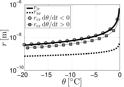
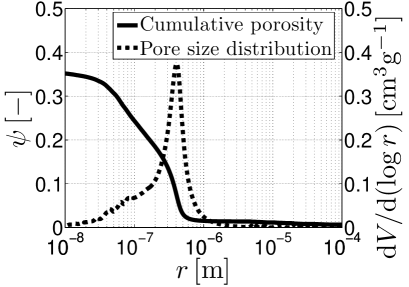
(a)	(b)

Figure 3: (a) Critical pore radius $r_{\mathrm{cr}}$ as a function of temperature, (b) pore size distribution obtained by mercury porosimetry and resulting cumulative porosity

The concept of the pore pressure caused by the ice crystals is well known, see [3, 4, 5, 14, 19, 20, 22, 27, 28]. To be more specific, let us consider spherical liquid-ice interface at the entrance of the pore and cylindrical shape of pores. Two interface equilibrium conditions are assumed to describe the interaction between ice crystals and pore walls. The Laplace relation is applicable to control the interface between the ice crystal and the liquid water:

$$p_{\mathrm{i}}-p_{\mathrm{l}}=\frac{2\gamma_{\mathrm{li}}}{r_{\mathrm{ir}}(\theta)},$$ (22)

where $p_{\mathrm{l}}\,\mathrm{[Pa]}$ is the liquid pressure and $p_{\mathrm{i}}\,\mathrm{[Pa]}$ is the pressure in the ice crystal. The second interface relation is expressed in the form of mechanical equilibrium between the ice crystal and the pore pressure exerted by the ice crystal, $p_{\mathrm{p}}\,\mathrm{[Pa]}$, as

$$p_{\mathrm{i}}-p_{\mathrm{p}}=\frac{\gamma_{\mathrm{li}}}{r-r_{\mathrm{ar}}(\theta)}.$$ (23)

Finally, combining Eq. (22) and Eq. (23), we can write

$$p_{\mathrm{p}}=p_{\mathrm{l}}+\chi(r,\theta),$$ (24)

where $\chi(r,\theta)\,\mathrm{[Pa]}$ is the local pressure on the frozen pore walls due to the ice formation and it is characterized by following relation, see [18, 28],

$$\chi(r,\theta)=\gamma_{\mathrm{li}}\left(\frac{2}{r_{\mathrm{ir}}(\theta)}-\frac{1}{r-r_{\mathrm{ar}}(\theta)}\right).$$ (25)

It has been advocated in  [19] and  [28] that the average pore pressure exerted by the ice crystal on the pore walls can be introduced as

$$p_{\mathrm{p}}=p_{\mathrm{l}}+\frac{1}{n}\int_{r_{\mathrm{cr}}(\theta)}^{\infty}\chi(r,\theta)\frac{\mathrm{d}\psi}{\mathrm{d}r}\,\mathrm{d}r,$$ (26)

where $n\,\mathrm{[-]}$ is the total porosity and $\psi(r)\,\mathrm{[-]}$ is the cumulative porosity. The cumulative porosity $\psi\,\mathrm{[-]}$ with a pore radius greater than $r\,\mathrm{[m]}$ is defined as, see Fig. 3(b),

$$\psi(r)=\int_{r}^{\infty}\frac{\mathrm{d}\psi}{\mathrm{d}r}\,\mathrm{d}r.$$ (27)

2.3 Mechanical (damage) model

The description of mechanical behavior of a porous media saturated with a liquid water was firstly proposed by Biot [2] and extended in the more general context of continuum thermodynamics for the ice crystals by Coussy [3, 4]. According to this approach, the formula between the effective stress $\mathchoice{\displaystyle\boldsymbol{\sigma}}{\textstyle\boldsymbol{\sigma}}{\scriptstyle\boldsymbol{\sigma}}{\scriptscriptstyle\boldsymbol{\sigma}}^{\prime}\,\mathrm{[Pa]}$ and total stress $\mathchoice{\displaystyle\boldsymbol{\sigma}}{\textstyle\boldsymbol{\sigma}}{\scriptstyle\boldsymbol{\sigma}}{\scriptscriptstyle\boldsymbol{\sigma}}\,\mathrm{[Pa]}$ has following form

$$\mathchoice{\displaystyle\boldsymbol{\sigma}}{\textstyle\boldsymbol{\sigma}}{\scriptstyle\boldsymbol{\sigma}}{\scriptscriptstyle\boldsymbol{\sigma}}=\mathchoice{\displaystyle\boldsymbol{\sigma}}{\textstyle\boldsymbol{\sigma}}{\scriptstyle\boldsymbol{\sigma}}{\scriptscriptstyle\boldsymbol{\sigma}}^{\prime}-bp_{\mathrm{p}}\mathchoice{\displaystyle\boldsymbol{i}}{\textstyle\boldsymbol{i}}{\scriptstyle\boldsymbol{i}}{\scriptscriptstyle\boldsymbol{i}},$$ (28)

where $b\,\mathrm{[-]}$ is Biot’s coefficient, $p_{\mathrm{p}}\,\mathrm{[Pa]}$ is the pressure exerted by ice crystal on the pore walls and $\mathchoice{\displaystyle\boldsymbol{i}}{\textstyle\boldsymbol{i}}{\scriptstyle\boldsymbol{i}}{\scriptscriptstyle\boldsymbol{i}}=\{1,1,1,0,0,0\}^{\sf T}$. The standard formulation of Biot’s coefficient related to the liquid water is based on introduction of the bulk modulus of porous material $K\,\mathrm{[Pa]}$ and the bulk modulus of solid matrix $K_{\mathrm{s}}\,\mathrm{[Pa]}$. For our purpose, we utilize more convenient relation for porous system derived in  [22] .

$$b=\frac{2n}{n+1}\approx 1-\frac{K}{K_{\mathrm{s}}},$$ (29)

where $n\,\mathrm{[-]}$ is the total porosity. As a further extension, we introduce one parameter isotropic nonlocal damage model given by constitutive law, see [1, 7],

$$\mathchoice{\displaystyle\boldsymbol{\sigma}}{\textstyle\boldsymbol{\sigma}}{\scriptstyle\boldsymbol{\sigma}}{\scriptscriptstyle\boldsymbol{\sigma}}^{\prime}=(1-d_{w})\mathchoice{\displaystyle\mathbf{D}}{\textstyle\mathbf{D}}{\scriptstyle\mathbf{D}}{\scriptscriptstyle\mathbf{D}}_{e}\mathchoice{\displaystyle\boldsymbol{\varepsilon}}{\textstyle\boldsymbol{\varepsilon}}{\scriptstyle\boldsymbol{\varepsilon}}{\scriptscriptstyle\boldsymbol{\varepsilon}},$$ (30)

damage law

$$d_{w}=g(\kappa)$$ (31)

and loading-unloading conditions

$$f(\mathchoice{\displaystyle\boldsymbol{\varepsilon}}{\textstyle\boldsymbol{\varepsilon}}{\scriptstyle\boldsymbol{\varepsilon}}{\scriptscriptstyle\boldsymbol{\varepsilon}},\kappa)=\varepsilon_{\mathrm{eq}}(\mathchoice{\displaystyle\boldsymbol{\varepsilon}}{\textstyle\boldsymbol{\varepsilon}}{\scriptstyle\boldsymbol{\varepsilon}}{\scriptscriptstyle\boldsymbol{\varepsilon}})-\kappa\leq 0,\qquad\dot{\kappa}\geq 0,\qquad f(\mathchoice{\displaystyle\boldsymbol{\varepsilon}}{\textstyle\boldsymbol{\varepsilon}}{\scriptstyle\boldsymbol{\varepsilon}}{\scriptscriptstyle\boldsymbol{\varepsilon}},\kappa)\dot{\kappa}=0,$$ (32)

where $\mathchoice{\displaystyle\mathbf{D}}{\textstyle\mathbf{D}}{\scriptstyle\mathbf{D}}{\scriptscriptstyle\mathbf{D}}_{e}\,\mathrm{[Pa]}$ is the elastic stiffness matrix, $d_{w}\,\mathrm{[-]}$ is the damage parameter, $\kappa\,\mathrm{[-]}$ is the internal variable corresponding to the maximum value of equivalent strain $\varepsilon_{\mathrm{eq}}\,\mathrm{[-]}$ reached in the loading history. The equivalent strain can be expressed in Mazars’s form as

$$\varepsilon_{\mathrm{eq}}=\sqrt{\sum_{I=1}^{3}\langle\varepsilon_{I}\rangle^{2}},$$ (33)

where $\varepsilon_{I}\,\mathrm{[-]}$ is component of the principal strains and the brackets denote the positive part. According to  [1], the local value $\varepsilon_{\mathrm{eq}}\,\mathrm{[-]}$ is replaced by its nonlocal average defined as

$$\varepsilon_{\mathrm{eq,nonlocal}}(\mathchoice{\displaystyle\boldsymbol{x}}{\textstyle\boldsymbol{x}}{\scriptstyle\boldsymbol{x}}{\scriptscriptstyle\boldsymbol{x}})=\int_{V}\phi(\mathchoice{\displaystyle\boldsymbol{x}}{\textstyle\boldsymbol{x}}{\scriptstyle\boldsymbol{x}}{\scriptscriptstyle\boldsymbol{x}},\mathchoice{\displaystyle\boldsymbol{\xi}}{\textstyle\boldsymbol{\xi}}{\scriptstyle\boldsymbol{\xi}}{\scriptscriptstyle\boldsymbol{\xi}})\varepsilon_{\mathrm{eq}}(\mathchoice{\displaystyle\boldsymbol{\xi}}{\textstyle\boldsymbol{\xi}}{\scriptstyle\boldsymbol{\xi}}{\scriptscriptstyle\boldsymbol{\xi}})\mathrm{d}\mathchoice{\displaystyle\boldsymbol{\xi}}{\textstyle\boldsymbol{\xi}}{\scriptstyle\boldsymbol{\xi}}{\scriptscriptstyle\boldsymbol{\xi}},$$ (34)

where $\phi(\mathchoice{\displaystyle\boldsymbol{x}}{\textstyle\boldsymbol{x}}{\scriptstyle\boldsymbol{x}}{\scriptscriptstyle\boldsymbol{x}},\mathchoice{\displaystyle\boldsymbol{\xi}}{\textstyle\boldsymbol{\xi}}{\scriptstyle\boldsymbol{\xi}}{\scriptscriptstyle\boldsymbol{\xi}})\,\mathrm{[-]}$ is the nonlocal weight function representing distance in the domain between the source point $\mathchoice{\displaystyle\boldsymbol{\xi}}{\textstyle\boldsymbol{\xi}}{\scriptstyle\boldsymbol{\xi}}{\scriptscriptstyle\boldsymbol{\xi}}\,\mathrm{[m]}$ and target point $\mathchoice{\displaystyle\boldsymbol{x}}{\textstyle\boldsymbol{x}}{\scriptstyle\boldsymbol{x}}{\scriptscriptstyle\boldsymbol{x}}\,\mathrm{[m]}$. For more details about nonlocal formulation we refer to [1]. Finally, the damage law $d_{w}=g(\kappa)$ is provided by following relation

$$g(\kappa)=\left\{\begin{array}[]{ll}0&\mathrm{for}\,\,0\leq\kappa\leq\varepsilon_{0},\\ 1-\frac{\kappa-\varepsilon_{0}}{\varepsilon_{f}-\varepsilon_{0}}&\mathrm{for}\,\,\varepsilon_{0}\leq\kappa\leq\varepsilon_{f},\\ 1&\mathrm{for}\,\,\varepsilon_{f}\leq\kappa.\end{array}\right.,$$ (35)

where $\varepsilon_{f}\,\mathrm{[-]}$ is the equivalent strain at critical crack opening and $\varepsilon_{0}\,\mathrm{[-]}$ is the strain at the elastic limit.

Considering the stress relation Eq. (28) and Eq. (30), the linear momentum balance equation for the porous system, can be expressed in the following form:

$$\mathchoice{\displaystyle\boldsymbol{\nabla}}{\textstyle\boldsymbol{\nabla}}{\scriptstyle\boldsymbol{\nabla}}{\scriptscriptstyle\boldsymbol{\nabla}}\cdot[\mathchoice{\displaystyle\boldsymbol{\sigma}}{\textstyle\boldsymbol{\sigma}}{\scriptstyle\boldsymbol{\sigma}}{\scriptscriptstyle\boldsymbol{\sigma}}^{\prime}-bp_{\mathrm{p}}\mathchoice{\displaystyle\boldsymbol{i}}{\textstyle\boldsymbol{i}}{\scriptstyle\boldsymbol{i}}{\scriptscriptstyle\boldsymbol{i}}]+\mathchoice{\displaystyle\boldsymbol{b}}{\textstyle\boldsymbol{b}}{\scriptstyle\boldsymbol{b}}{\scriptscriptstyle\boldsymbol{b}}=0,$$ (36)

where $\mathchoice{\displaystyle\boldsymbol{b}}{\textstyle\boldsymbol{b}}{\scriptstyle\boldsymbol{b}}{\scriptscriptstyle\boldsymbol{b}}\,\mathrm{[Nm^{-3}]}$ is the body force. The governing equations are discretized in space using the standard finite element approximation. The unknown displacement field $\mathchoice{\displaystyle\boldsymbol{u}}{\textstyle\boldsymbol{u}}{\scriptstyle\boldsymbol{u}}{\scriptscriptstyle\boldsymbol{u}}\,\mathrm{[m]}$ is expressed in terms of its nodal values. Details of the formulation may be found in [6].

2.4 Boundary and initial conditions

To complete the proposed material model, the initial and boundary conditions are set as follows:

• The Dirichlet boundary conditions

  $$\theta = \hat{\theta}(t)\quad\mathrm{on}\quad\Gamma_{\theta}^{\mathrm{I}},$$

  $$\varphi = \hat{\varphi}(t)\quad\mathrm{on}\quad\Gamma_{\varphi}^{\mathrm{I}},$$ (37)

  $$\mathchoice{\displaystyle\boldsymbol{u}}{\textstyle\boldsymbol{u}}{\scriptstyle\boldsymbol{u}}{\scriptscriptstyle\boldsymbol{u}} = \hat{\mathchoice{\displaystyle\boldsymbol{u}}{\textstyle\boldsymbol{u}}{\scriptstyle\boldsymbol{u}}{\scriptscriptstyle\boldsymbol{u}}}(t)\quad\mathrm{on}\quad\Gamma_{u}^{\mathrm{I}},$$

• The Neumann boundary conditions

  $${[-\lambda\mathchoice{\displaystyle\boldsymbol{\nabla}}{\textstyle\boldsymbol{\nabla}}{\scriptstyle\boldsymbol{\nabla}}{\scriptscriptstyle\boldsymbol{\nabla}}\theta-\delta_{\mathrm{v}}\mathchoice{\displaystyle\boldsymbol{\nabla}}{\textstyle\boldsymbol{\nabla}}{\scriptstyle\boldsymbol{\nabla}}{\scriptscriptstyle\boldsymbol{\nabla}}\{\varphi p_{\mathrm{sat}}(\theta)\}]}\cdot\mathchoice{\displaystyle\boldsymbol{n}}{\textstyle\boldsymbol{n}}{\scriptstyle\boldsymbol{n}}{\scriptscriptstyle\boldsymbol{n}} = q_{\mathrm{h}}(t)+q_{\mathrm{h,swr}}(t)\quad\mathrm{on}\quad\Gamma_{\theta}^{\mathrm{II}},$$

  $${[-D_{\varphi}\mathchoice{\displaystyle\boldsymbol{\nabla}}{\textstyle\boldsymbol{\nabla}}{\scriptstyle\boldsymbol{\nabla}}{\scriptscriptstyle\boldsymbol{\nabla}}\varphi-\delta_{\mathrm{v}}\mathchoice{\displaystyle\boldsymbol{\nabla}}{\textstyle\boldsymbol{\nabla}}{\scriptstyle\boldsymbol{\nabla}}{\scriptscriptstyle\boldsymbol{\nabla}}\{\varphi p_{\mathrm{sat}}(\theta)\}]}\cdot\mathchoice{\displaystyle\boldsymbol{n}}{\textstyle\boldsymbol{n}}{\scriptstyle\boldsymbol{n}}{\scriptscriptstyle\boldsymbol{n}} = q_{\mathrm{v}}(t)+q_{\mathrm{l}}(t)+q_{\mathrm{l,rain}}(t)\quad\mathrm{on}\quad\Gamma_{\varphi}^{\mathrm{II}},$$

  $$\mathchoice{\displaystyle\boldsymbol{\sigma}}{\textstyle\boldsymbol{\sigma}}{\scriptstyle\boldsymbol{\sigma}}{\scriptscriptstyle\boldsymbol{\sigma}}^{\prime}\cdot\mathchoice{\displaystyle\boldsymbol{n}}{\textstyle\boldsymbol{n}}{\scriptstyle\boldsymbol{n}}{\scriptscriptstyle\boldsymbol{n}} = \mathchoice{\displaystyle\boldsymbol{\sigma}}{\textstyle\boldsymbol{\sigma}}{\scriptstyle\boldsymbol{\sigma}}{\scriptscriptstyle\boldsymbol{\sigma}}_{\mathrm{t}}(t)\quad\mathrm{on}\quad\Gamma_{u}^{\mathrm{II}},$$ (38)

• The Robin boundary conditions

  $${[-\lambda\mathchoice{\displaystyle\boldsymbol{\nabla}}{\textstyle\boldsymbol{\nabla}}{\scriptstyle\boldsymbol{\nabla}}{\scriptscriptstyle\boldsymbol{\nabla}}\theta-\delta_{\mathrm{v}}\mathchoice{\displaystyle\boldsymbol{\nabla}}{\textstyle\boldsymbol{\nabla}}{\scriptstyle\boldsymbol{\nabla}}{\scriptscriptstyle\boldsymbol{\nabla}}\{\varphi p_{\mathrm{sat}}(\theta)\}]}\cdot\mathchoice{\displaystyle\boldsymbol{n}}{\textstyle\boldsymbol{n}}{\scriptstyle\boldsymbol{n}}{\scriptscriptstyle\boldsymbol{n}} = \alpha_{\mathrm{h}}{[\theta-\theta_{\infty}(t)]}\quad\mathrm{on}\quad\Gamma_{\theta}^{\mathrm{III}},$$

  $${[-D_{\varphi}\mathchoice{\displaystyle\boldsymbol{\nabla}}{\textstyle\boldsymbol{\nabla}}{\scriptstyle\boldsymbol{\nabla}}{\scriptscriptstyle\boldsymbol{\nabla}}\varphi-\delta_{\mathrm{v}}\mathchoice{\displaystyle\boldsymbol{\nabla}}{\textstyle\boldsymbol{\nabla}}{\scriptstyle\boldsymbol{\nabla}}{\scriptscriptstyle\boldsymbol{\nabla}}\{\varphi p_{\mathrm{sat}}(\theta)\}]}\cdot\mathchoice{\displaystyle\boldsymbol{n}}{\textstyle\boldsymbol{n}}{\scriptstyle\boldsymbol{n}}{\scriptscriptstyle\boldsymbol{n}} = \beta_{\mathrm{v}}{[\varphi-\varphi_{\infty}(t)]}\quad\mathrm{on}\quad\Gamma_{\varphi}^{\mathrm{III}},$$ (39)

• Initial conditions

  $$\theta(\mathchoice{\displaystyle\boldsymbol{x}}{\textstyle\boldsymbol{x}}{\scriptstyle\boldsymbol{x}}{\scriptscriptstyle\boldsymbol{x}},0)=\theta_{\mathrm{in}}\quad\varphi(\mathchoice{\displaystyle\boldsymbol{x}}{\textstyle\boldsymbol{x}}{\scriptstyle\boldsymbol{x}}{\scriptscriptstyle\boldsymbol{x}},0)=\varphi_{\mathrm{in}}\quad\mathchoice{\displaystyle\boldsymbol{u}}{\textstyle\boldsymbol{u}}{\scriptstyle\boldsymbol{u}}{\scriptscriptstyle\boldsymbol{u}}(\mathchoice{\displaystyle\boldsymbol{x}}{\textstyle\boldsymbol{x}}{\scriptstyle\boldsymbol{x}}{\scriptscriptstyle\boldsymbol{x}},0)=\mathchoice{\displaystyle\boldsymbol{u}}{\textstyle\boldsymbol{u}}{\scriptstyle\boldsymbol{u}}{\scriptscriptstyle\boldsymbol{u}}_{\mathrm{in}}\quad\mathrm{for}\,\,\mathrm{all}\quad\mathchoice{\displaystyle\boldsymbol{x}}{\textstyle\boldsymbol{x}}{\scriptstyle\boldsymbol{x}}{\scriptscriptstyle\boldsymbol{x}}\in\Omega,$$ (40)

where the symbol $\,\hat{\cdot}\,$ denotes prescribed value, $\mathchoice{\displaystyle\boldsymbol{n}}{\textstyle\boldsymbol{n}}{\scriptstyle\boldsymbol{n}}{\scriptscriptstyle\boldsymbol{n}}\,\mathrm{[-]}$ is the unit normal vector, $q_{\mathrm{h,swr}}\,\mathrm{[Wm^{-2}]}$ is the solar short-wave radiation flux, $q_{\mathrm{l,rain}}\,\mathrm{[kgm^{-2}s^{-1}]}$ is the driving-rain flux, $\mathchoice{\displaystyle\boldsymbol{\sigma}}{\textstyle\boldsymbol{\sigma}}{\scriptstyle\boldsymbol{\sigma}}{\scriptscriptstyle\boldsymbol{\sigma}}_{\mathrm{t}}\,\mathrm{[Pa]}$ is the imposed traction, $\alpha_{\mathrm{h}}\,\mathrm{[Wm^{-2}K^{-1}]}$ is the heat transfer coefficient, $\beta_{\mathrm{v}}\,\mathrm{[kgm^{-2}s^{-1}Pa^{-1}]}$ is the water vapor transfer coefficient, $\theta_{\infty}$ and $\varphi_{\infty}$ are the ambient temperature and moisture, respectively.

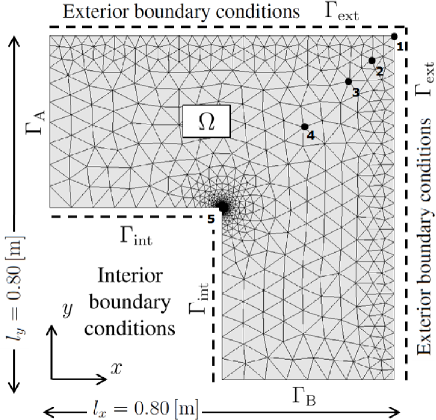
Figure 4: $2$-D domain with initial and boundary conditions

3 Numerical example

In this section, we employ the proposed thermo-hygro-mechanical model to perform a numerical simulation of transport processes below freezing point in porous media and their impact on the mechanical properties. In doing so we consider geometry together with the initial and loading conditions displayed in Fig 4. Two-dimensional L-shape domain was discretized by an FE mesh into $741$ nodes and $1358$ triangular elements. The solution of the time-dependent problem also involves a discretization of the time domain into $744$ uniform time steps chosen with regard to the convergence criteria of nonlinear solution.

Symbol	Unit		Value	Ref.
Transport properties of mortar
$w_{f}$	$\mathrm{[kgm^{-3}]}$	free water saturation	160	[23]
$w_{\mathrm{80}}$	$\mathrm{[kgm^{-3}]}$	water content at $\varphi=0.8$ [-]	23	[23]
$\lambda_{\mathrm{0}}$	$\mathrm{[Wm^{-1}K^{-1}]}$	thermal conductivity	0.45	[23]
$b_{\mathrm{tcs}}$	$\mathrm{[-]}$	thermal conductivity supplement	9	[23]
$\rho_{\mathrm{s}}$	$\mathrm{[kgm^{-3}]}$	bulk density	1670	[23]
$\mu$	$\mathrm{[-]}$	water vapor diffusion resistance factor	9.63	[17, 23]
$a$	$\mathrm{[kgm^{-2}s^{-0.5}]}$	water absorption coefficient	0.82	[17, 23]
$c_{\mathrm{s}}$	$\mathrm{[Jkg^{-1}K^{-1}]}$	specific heat capacity	1000	[17, 23]
Mechanical properties of mortar
$E$	$\mathrm{[Pa]}$	Young’s modulus	$1\cdot 10^{10}$	[15, 16]
$\nu$	$\mathrm{[-]}$	Poisson’s ratio	0.2	[15, 16]
$f_{t}$	$\mathrm{[Pa]}$	tensile strength	$2.5\cdot 10^{6}$	[15, 16]
$\varepsilon_{f}$	$\mathrm{[-]}$	equivalent strain at critical crack opening	$2.5\cdot 10^{-3}$	[1, 7]
$l_{\mathrm{intl}}$	$\mathrm{[m]}$	internal length	$1\cdot 10^{-3}$	[1, 7]
$\alpha$	$\mathrm{[K^{-1}]}$	thermal expansion coefficient	$1.2\cdot 10^{-5}$	[15, 16]
Ice formation process
$\gamma_{\mathrm{li}}$	$\mathrm{[Nm^{-1}]}$	liquid/ice surface tension	0.0409	[13]
$\Delta s_{\mathrm{m}}$	$\mathrm{[PaK^{-1}]}$	melting entropy	$1.2\cdot 10^{6}$	[13]
$n$	$\mathrm{[-]}$	total porosity	0.35	[17, 21]
$\psi$	$\mathrm{[-]}$	cumulative volume of pores	Fig. 3(b)	[17, 21]
Other properties
$\alpha_{\mathrm{h}}$	$\mathrm{[Wm^{-2}K^{-1}]}$	heat transfer coefficient	8	[10]
$\beta_{\mathrm{v}}$	$\mathrm{[kgm^{-2}s^{-1}Pa^{-1}]}$	water vapor transfer coefficient	$5.6\cdot 10^{-8}$	[10]
$\alpha_{\mathrm{swr}}$	$\mathrm{[-]}$	short-wave absorption coefficient	0.6	[10]

Table 1: Input parameters of numerical simulation

The measured material parameters, corresponding to a lime mortar, are listed in Tab. 1. Several parameters were obtained from a set of experimental measurements providing mostly the hygric and thermal properties of mortar, see  [17]. Unfortunately, no additional experiments were conducted for the mechanical properties, hence we utilize some material parameters of mortars mentioned in the literature, see Tab. 1.

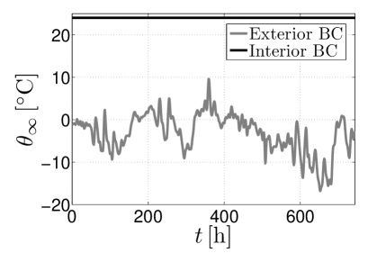
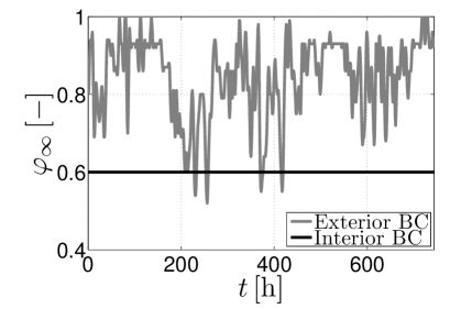
(a)	(b)
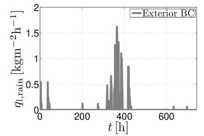
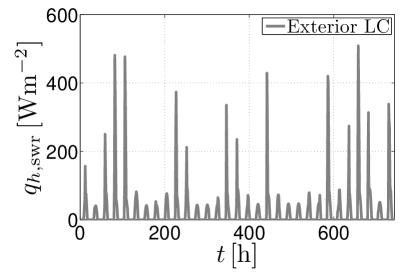
(c)	(d)

Figure 5: Exterior and interior boundary conditions - (a) temperature, (b) moisture, (c) driving-rain, (d) short-wave radiation

The initial conditions were set equal to $\mathchoice{\displaystyle\boldsymbol{u}}{\textstyle\boldsymbol{u}}{\scriptstyle\boldsymbol{u}}{\scriptscriptstyle\boldsymbol{u}}_{\mathrm{in}}=\mathchoice{\displaystyle\boldsymbol{0}}{\textstyle\boldsymbol{0}}{\scriptstyle\boldsymbol{0}}{\scriptscriptstyle\boldsymbol{0}}\,\mathrm{[m]}$, $\theta_{\mathrm{in}}=14\,\mathrm{[^{\circ}C]}$ and $\varphi_{\mathrm{in}}=0.5\,\mathrm{[-]}$ in the whole domain. The following Robin boundary conditions were imposed: on the interior side a constant temperature of $24\,\mathrm{[^{\circ}C]}$ and a constant relative humidity $0.6\,\mathrm{[-]}$ were maintained, while on the exterior side the real climatic data representing the winter conditions were prescribed, see Figs. 5(a),(b). Moreover, the exterior side of the domain was loaded by the heat flux from solar short-wave radiation $q_{\mathrm{h,swr}}\,\mathrm{[Wm^{-2}]}$ and the driving-rain flux $q_{\mathrm{l,rain}}\,\mathrm{[kgm^{-2}s^{-1}]}$ (the Neumann boundary conditions), see Figs. 5(c),(d) and Tab. 2.

Side	BC type	Description	Fig.
Boundary conditions
$\Gamma_{\mathrm{ext}}$	II	${[-\lambda\mathchoice{\displaystyle\boldsymbol{\nabla}}{\textstyle\boldsymbol{\nabla}}{\scriptstyle\boldsymbol{\nabla}}{\scriptscriptstyle\boldsymbol{\nabla}}\theta-\delta_{\mathrm{v}}\mathchoice{\displaystyle\boldsymbol{\nabla}}{\textstyle\boldsymbol{\nabla}}{\scriptstyle\boldsymbol{\nabla}}{\scriptscriptstyle\boldsymbol{\nabla}}\{\varphi p_{\mathrm{sat}}(\theta)\}]}\cdot\mathchoice{\displaystyle\boldsymbol{n}}{\textstyle\boldsymbol{n}}{\scriptstyle\boldsymbol{n}}{\scriptscriptstyle\boldsymbol{n}}=q_{\mathrm{h,swr}}(t)$	5(d)
$\Gamma_{\mathrm{ext}}$	II	${[-D_{\varphi}\mathchoice{\displaystyle\boldsymbol{\nabla}}{\textstyle\boldsymbol{\nabla}}{\scriptstyle\boldsymbol{\nabla}}{\scriptscriptstyle\boldsymbol{\nabla}}\varphi-\delta_{\mathrm{v}}\mathchoice{\displaystyle\boldsymbol{\nabla}}{\textstyle\boldsymbol{\nabla}}{\scriptstyle\boldsymbol{\nabla}}{\scriptscriptstyle\boldsymbol{\nabla}}\{\varphi p_{\mathrm{sat}}(\theta)\}]}\cdot\mathchoice{\displaystyle\boldsymbol{n}}{\textstyle\boldsymbol{n}}{\scriptstyle\boldsymbol{n}}{\scriptscriptstyle\boldsymbol{n}}=q_{\mathrm{l,rain}}(t)$	5(c)
$\Gamma_{\mathrm{ext}}$	III	${[-\lambda\mathchoice{\displaystyle\boldsymbol{\nabla}}{\textstyle\boldsymbol{\nabla}}{\scriptstyle\boldsymbol{\nabla}}{\scriptscriptstyle\boldsymbol{\nabla}}\theta-\delta_{\mathrm{v}}\mathchoice{\displaystyle\boldsymbol{\nabla}}{\textstyle\boldsymbol{\nabla}}{\scriptstyle\boldsymbol{\nabla}}{\scriptscriptstyle\boldsymbol{\nabla}}\{\varphi p_{\mathrm{sat}}(\theta)\}]}\cdot\mathchoice{\displaystyle\boldsymbol{n}}{\textstyle\boldsymbol{n}}{\scriptstyle\boldsymbol{n}}{\scriptscriptstyle\boldsymbol{n}}=8{[\theta-\theta_{\infty}(t)]}$	5(a)
$\Gamma_{\mathrm{ext}}$	III	${[-D_{\varphi}\mathchoice{\displaystyle\boldsymbol{\nabla}}{\textstyle\boldsymbol{\nabla}}{\scriptstyle\boldsymbol{\nabla}}{\scriptscriptstyle\boldsymbol{\nabla}}\varphi-\delta_{\mathrm{v}}\mathchoice{\displaystyle\boldsymbol{\nabla}}{\textstyle\boldsymbol{\nabla}}{\scriptstyle\boldsymbol{\nabla}}{\scriptscriptstyle\boldsymbol{\nabla}}\{\varphi p_{\mathrm{sat}}(\theta)\}]}\cdot\mathchoice{\displaystyle\boldsymbol{n}}{\textstyle\boldsymbol{n}}{\scriptstyle\boldsymbol{n}}{\scriptscriptstyle\boldsymbol{n}}=5.6\cdot 10^{-8}{[\varphi-\varphi_{\infty}(t)]}$	5(b)
$\Gamma_{\mathrm{int}}$	III	${[-\lambda\mathchoice{\displaystyle\boldsymbol{\nabla}}{\textstyle\boldsymbol{\nabla}}{\scriptstyle\boldsymbol{\nabla}}{\scriptscriptstyle\boldsymbol{\nabla}}\theta-\delta_{\mathrm{v}}\mathchoice{\displaystyle\boldsymbol{\nabla}}{\textstyle\boldsymbol{\nabla}}{\scriptstyle\boldsymbol{\nabla}}{\scriptscriptstyle\boldsymbol{\nabla}}\{\varphi p_{\mathrm{sat}}(\theta)\}]}\cdot\mathchoice{\displaystyle\boldsymbol{n}}{\textstyle\boldsymbol{n}}{\scriptstyle\boldsymbol{n}}{\scriptscriptstyle\boldsymbol{n}}=8{[\theta-24]}$	5(a)
$\Gamma_{\mathrm{int}}$	III	${[-D_{\varphi}\mathchoice{\displaystyle\boldsymbol{\nabla}}{\textstyle\boldsymbol{\nabla}}{\scriptstyle\boldsymbol{\nabla}}{\scriptscriptstyle\boldsymbol{\nabla}}\varphi-\delta_{\mathrm{v}}\mathchoice{\displaystyle\boldsymbol{\nabla}}{\textstyle\boldsymbol{\nabla}}{\scriptstyle\boldsymbol{\nabla}}{\scriptscriptstyle\boldsymbol{\nabla}}\{\varphi p_{\mathrm{sat}}(\theta)\}]}\cdot\mathchoice{\displaystyle\boldsymbol{n}}{\textstyle\boldsymbol{n}}{\scriptstyle\boldsymbol{n}}{\scriptscriptstyle\boldsymbol{n}}=5.6\cdot 10^{-8}{[\varphi-0.6]}$	5(b)
$\Gamma_{\mathrm{A}}$	I	$u_{x}(t)=0\,\mathrm{[m]}$
$\Gamma_{\mathrm{B}}$	I	$u_{y}(t)=0\,\mathrm{[m]}$
Initial conditions
$\Omega$		$\theta_{\mathrm{in}}=14\,\mathrm{[^{\circ}C]}$
$\Omega$		$\varphi_{\mathrm{in}}=0.5\,\mathrm{[-]}$
$\Omega$		$\mathchoice{\displaystyle\boldsymbol{u}}{\textstyle\boldsymbol{u}}{\scriptstyle\boldsymbol{u}}{\scriptscriptstyle\boldsymbol{u}}_{\mathrm{in}}=\mathchoice{\displaystyle\boldsymbol{0}}{\textstyle\boldsymbol{0}}{\scriptstyle\boldsymbol{0}}{\scriptscriptstyle\boldsymbol{0}}\,\mathrm{[m]}$

Table 2: Boundary and initial conditions

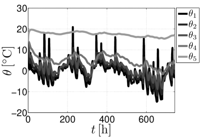
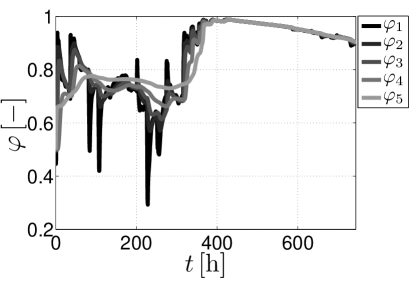
(a)	(b)

Figure 6: (a) Resulting temperature at selected nodes, (b) resulting moisture at selected nodes

The results are presented in Fig. 6 showing variation of the temperature and moisture at selected nodes labeled in Fig. 4. The obtained results clearly manifesting the influence of exterior boundary conditions on the temperature and moisture fields, especially near the exterior surface of the $2$-D domain.

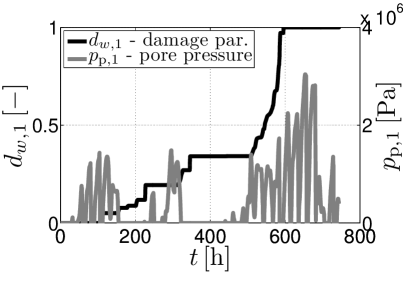
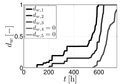
(a)	(b)

Figure 7: (a) Evolution of damage parameter $d_{w,1}\,\mathrm{[-]}$ and pore pressure $p_{\mathrm{p},1}\,\mathrm{[Pa]}$ at node $1$, (b) Evolution of damage parameters $d_{w}\,\mathrm{[-]}$ at selected nodes

Several interesting results have been derived within the scope of the calculation of internal damage. Figs. 7(a),(b) display the evolution of damage parameter and its dependence on the average pore pressure. Beside the comparison of the evolution of damage parameter in the time, we also compare growth of damage parameter in the domain, see Fig. 8. Analysis of these results allows better understanding of physical phenomena in porous media subjected to the frost action. A fast moisture increase in the zone close to the exterior surface (Fig. 6(b)) leads also to the similar trend of the damage parameter, see Fig. 7(a). This can be attributed to the lower exterior temperature and higher moisture content in the surface layer caused by the driving-rain flux. It is evident from the boundary conditions plotted in Figs. 5(a),(c). The calculated results promote the capability of proposed governing equations to simulate a degradation processes in the building materials exposed to real weather conditions.

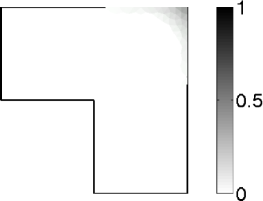
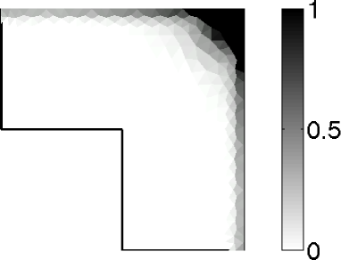
(a)	(b)

Figure 8: (a) Evolution of damage parameter $d_{w}\,\mathrm{[-]}$ after $t=372\,\mathrm{[h]}$, (b) evolution of damage parameter $d_{w}\,\mathrm{[-]}$ at the end of analyzed time period ($t=744\,\mathrm{[h]}$)

3.1 Influence of porosity

The formation of ice is mainly controlled by pore size distribution, see  [28]. To address this issue we consider the same input data as in the previous numerical example except for the total porosity $n\,\mathrm{[-]}$ and cumulative porosity $\psi\,\mathrm{[-]}$. Note that the structure of porous system affects surely transport and mechanical properties of mortars, but we focus here only on the influence of different porosity to keep the numerical study clear and transparent, see Eqs. (26) and (36). Therefore, two different pore size distributions were taken into account, see Fig. 9(a). Further we assume in calculations the following values of total porosity $\{n_{\mathrm{spec01}}=0.35\,\mathrm{[-]},n_{\mathrm{spec02}}=0.13\,\mathrm{[-]}\}$ representing material properties of the lime mortar and the lime mortars with oil additive, respectively.

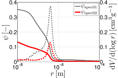
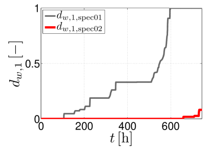
(a)	(b)
(c)	(d)

Figure 9: (a) Two different pore size distributions and cumulative porosity functions, (b) comparison of damage evolutions at node $1$, (c) evolution of damage parameter $d_{w,1,\mathrm{spec02}}\,\mathrm{[-]}$ and pore pressure $p_{\mathrm{p},1,\mathrm{spec02}}\,\mathrm{[Pa]}$ at node $1$ for porosity equal to $n_{\mathrm{spec02}}=0.13\,\mathrm{[-]}$, (d) evolution of damage parameter $d_{w,\mathrm{spec02}}\,\mathrm{[-]}$ at the end of analyzed time period ($t=744\,\mathrm{[h]}$)

For a given pore size distributions, Figs. 9(b), (d) shows the evolution of damage parameters in the critical location of the $2$-D domain. It is shown that the value of total porosity changes slightly, while the influence on the evolution of damage parameter is significant. This is clearly observed from the comparison of pore pressures displayed in Fig. 7(a) and Fig. 9(c). Combining all the previous results suggests that the structure of porous system plays crucial role in the resulting pore pressure and subsequently calculated internal damage.

4 Conclusions

This paper presents the numerical modeling of damage caused by ice crystallization process in mortars. Attention is focused on the thermo-hygro-mechanical model developed here in the framework of uncoupled algorithmic scheme. Two particular issues were addressed: (i) the formulation of material model based on laws of the thermodynamics, poromechanics and damage mechanics, (ii) influence of porosity on the mechanical behavior.

In particular, we employed Künzel’s model, which is sufficiently robust to describe real-world materials, but which is also highly nonlinear, time-dependent material model. Supported by several successful applications in civil engineering we adopted Biot’s model and the nonlocal isotropic damage model in the framework to simulate the frost action on porous media.

A crucial point in modeling of damage in mortars is the pore size distribution. The obtained results suggest a high importance of porosity on evolution of the damage parameter, at least for the present material parameters and applied range of initial and boundary conditions.

Finally a comparison of the numerical calculations with experimental measurements is under current investigation and will be presented elsewhere.

Acknowledgement

This outcome has been achieved with the financial support of project NAKI - DF11P01OVV0080 entitled ”High-performance and compatible lime mortars for extreme application in restoration, repair and preventive maintenance of architectural heritage”. The experimental work performed at the Institute of Theoretical and Applied Mechanics AS CR under the leadership of Dr. Zuzana Slížková is also gratefully acknowledged.

References

- [1] Z. B. Bažant and J. Jirásek. Nonlocal integral formulations of plasticity and damage: Survey of progress. Journal of Engineering Mechanics, 128(11):1119–1149, 2002.
- [2] M. A. Biot. General theory of three-dimensional consolidation. Journal of Applied Physics, 12(2):155–164, 1941.
- [3] O. Coussy and P. Monteiro. Unsaturated poroelasticity for crystallization in pores. Computers and Geotechnics, 34(4):279–290, 2007.
- [4] O. Coussy and P. Monteiro. Poroelastic model for concrete exposed to freezing temperatures. Cement and Concrete Research, 38(1):40–48, 2008.
- [5] G. Fagerlund. Determination of pore-size distribution from freezing-point depression. Materials and Structures, 6(3):215–225, 1973.
- [6] D. Gawin, F. Pesavento, and B. A. Schrefler. Modelling of hygro-thermal behaviour of concrete at high temperature with thermo-chemical and mechanical material degradation. Computer Methods in Applied Mechanics and Engineering, 192(13):1731–1771, 2003.
- [7] M. Horák. Localization analysis of damage and plasticity models. Master’s thesis, CTU in Prague, 2009. in Czech.
- [8] F. Kong and H. Wang. Heat and mass coupled transfer combined with freezing process in building materials: Modeling and experimental verification. Energy and Building, 43(10):2850–2859, 2011.
- [9] M. Koster. 3D multi-scale model of moisture transport in cement-based materials. In W. Brameshuber, editor, International RILEM Conference on Material Science, pages 165–176, 2010.
- [10] H. M. Künzel and K. Kiessl. Calculation of heat and moisture transfer in exposed building components. International Journal of Heat and Mass Transfer, 40(1):159–167, 1996.
- [11] A. Kučerová and J. Sýkora. Uncertainty updating in the description of coupled heat and moisture transport in heterogeneous materials. Applied Mathematics and Computation, 219(13):7252 –7261, 2013.
- [12] R. W. Lewis and B. A. Schrefler. The Finite Element Method in the Static and Dynamic Deformation and Consolidation of Porous Media. John Wiley&Sons, Chichester, England, 2nd edition, 1999.
- [13] L. Liu, G. Ye, E. Schlagen, H. Chen, Z. Qian, W. Sun, and K. van Breugel. Modeling of the internal damage of saturated cement paste due to ice crystallization pressure during freezing. Cement and Concrete Research, 33(5):562–571, 2011.
- [14] S. Matala. Effects of carbonation on the pore structure of granulated blast furnace slag concrete. PhD thesis, Helsinki University of Technology, 1995.
- [15] G. Milani and A. Tralli. Simple lower bound limit analysis homogenization model for in- and out-of-plane loaded masonry walls. Construction and Building Materials, 25(12):808–834, 2012.
- [16] G. Milani and A. Tralli. A simple meso-macro model based on SQP for the non-linear analysis of masonry double curvature structures. International Journal of Solids and Structures, 49(4):1999–2011, 2012.
- [17] C. Nunes, Z. Slížková, D. Křiánková, and D. Frankeová. Effect of linseed oil on the mechanical properties of lime mortars. In Engineering Mechanics 2012, 2012.
- [18] A. Sellier S. Multon and B. Perrin. Numerical analysis of frost effects in porous media. Benefits and limits of the finite element poroelasticity formulation. International Journal for Numerical and Analytical Methods in Geomechanics, 36(4):438–458, 2012.
- [19] G. W. Scherer. Freezing gels. Journal of Non-Crystalline Solids, 155(1):1–25, 1993.
- [20] G. W. Scherer. Crystallization in pores. Cement and Concrete Research, 29(8):1347 –1358, 1999.
- [21] Z. Slížková, M. Drdácký, D. Frankeová, L. Nosál, and A. Zeman. Study of historic mortars from Charles Bridge. In Restaurování a Ochrana Uměleckých děl IV, pages 26–28, 2010. in Czech.
- [22] Z. Sun and G. W. Scherer. Effect of air voids on salt scaling and internal freezing. Cement and Concrete Research, 40(2):260–270, 2010.
- [23] J. Sýkora, T. Krejčí, J. Kruis, and M. Šejnoha. Computational homogenization of non-stationary transport processes in masonry structures. Journal of Computational and Applied Mathematics, 18:4745 –4755, 2012.
- [24] J. Sýkora, M. Šejnoha, and J. Šejnoha. Homogenization of coupled heat and moisture transport in masonry structures including interfaces. Applied Mathematics and Computation, 219(13):7275– 7285, 2013.
- [25] X. Tan, W. Chen, H. Tian, and J. Cao. Water flow and heat transport including ice/water phase chase in porous media: Numerical simulation and application. Cold Regions and Technology, 68(1–2):74–84, 2011.
- [26] R. Černý and P. Rovnaníková. Transport Processes in Concrete. London: Spon Press, 2002.
- [27] G. Wardeh and B. Perrin. Numerical modelling of the behaviour of consolidated porous media exposed to frost action. Construction and Building Materials, 22(4):600– 608, 2008.
- [28] B. Zuber and J. Marchand. Modeling the deterioration of hydrated cement systems exposed to frost action - Part 1: Description of the mathematical model. Cement and Concrete Research, 30(12):1929–1939, 2000.