Investigation of the Galactic Bar Based on Photometry

and Stellar Proper Motions

V. V. Bobylev^1,2, A. V. Mosenkov^1,2, A. T. Bajkova¹, and G. A. Gontcharov¹

¹Pulkovo Astronomical Observatory, Russian Academy of Sciences,

Pulkovskoe sh. 65, St. Petersburg, 196140 Russia

²Sobolev Astronomical Institute, St. Petersburg State University,

Universitetskii pr. 28, Petrodvorets, 198504 Russia

Abstract – A new method for selecting stars in the Galactic bar based on 2MASS infrared photometry in combination with stellar proper motions from the Kharkiv XPM catalogue has been implemented. In accordance with this method, red clump and red giant branch stars are preselected on the color – magnitude diagram and their photometric distances are calculated. Since the stellar proper motions are indicators of a larger velocity dispersion toward the bar and the spiral arms compared to the stars with circular orbits, applying the constraints on the proper motions of the preselected stars that take into account the Galactic rotation has allowed the background stars to be eliminated. Based on a joint analysis of the velocities of the selected stars and their distribution on the Galactic plane, we have confidently identified the segment of the Galactic bar nearest to the Sun with an orientation of 20^∘–25^∘ with respect to the Galactic center – Sun direction and a semimajor axis of no more than 3 kpc.

DOI: 10.1134/S1063773714030037

Keywords: Galactic structure, central bar, spiral structure, red giant clump, red giant branch stars, stellar proper motions.

INTRODUCTION

The first evidence for the presence of a central bar in the Galaxy was probably provided by de Vaucouleurs (1970). Subsequently, observational proof of the existence of a bar was obtained in several ways. These include a study of the gas kinematics (Binney et al. 1991), analysis of the surface brightness (Blitz and Spergel 1991), star counts (Nakada et al. 1991; Stanek et al. 1994), and experiments on searching for microlensing (Udalski et al. 1994).

The appearance of infrared photometry for hundreds of millions of stars led to a considerable success in studying the Galactic bar. Analysis of the red giant clump from the 2MASS (Babusiaux and Gilmore 2005), OGLE-II (Rattenbury et al. 2007), and OGLE-III (Nataf et al. 2013) catalogues showed that the bar is oriented with respect to the Galactic center.Sun direction at an angle of 15^∘–45^∘, its radius is 3–4 kpc, and the ratio of its axes $(x_{b}:y_{b}:z_{b})$ is approximately 10 : 3.6 : 2.7 (Rattenbury et al. 2007). At present, the bar orientation parameters and sizes are being debated. Most authors incline to the model of a short bar ($R_{b}\approx 3$ kpc) oriented at an angle of about 20^∘. Other authors talk about a long bar ($R_{b}\approx 4$ 4 kpc) oriented at an angle of about 44^∘ (Benjamin et al. 2005; L$\acute{o}$pez – Corredoira et al. 2007).

We are going to use red clump and red giant branch stars as distance indicators. The method for selecting such stars was implemented by Gontcharov (2008, 2011) using the2MASS (Skrutskie et al. 2006) and Tycho-2 (Hog et al. 2000) catalogues as an example.

It is important to note that the motions of stars belonging to the bar have significant deviations from circular orbits. If we take many stars lying on the same line of sight (toward the bar) but located at different distances (at both near and far ends of the bar), then we will observe a considerable velocity dispersion.

Simulations of the bar kinematics show that there is a peak in the dispersions of both stellar line-of-sight velocities (Zhao 1996; Wang et al. 2012) and proper motions (Zhao 1996) in the direction $l=0^{\circ}$. We are going to use this fact for a more reliable selection of stars belonging to the Galactic bar. The line-of-sight velocities of stars are of greatest interest for such a task, because their values and errors do not depend on heliocentric distance. At present, however, there is no sufficient number of line-of-sight velocity measurements for the stars we need. Therefore, we are going to use the proper motions of stars.

The Kharkiv XPM catalogue (Fedorov et al. 2009, 2011), which contains the proper motions of $\sim$314 million stars and incorporates 2MASS infrared photometry, is quite suitable for these purposes. The fact that the XPM catalogue is an independent realization of the inertial reference frame is of particular interest. About 1.5 million galaxies were used to absolutize the stellar proper motions.

The spiral structure of the Galaxy is closely related to the bar. At present, however, there is no unequivocal answer even to the question about the number of spiral arms in the Galaxy. Analysis of the spatial distribution of young Galactic objects (young stars, star-forming regions, open star clusters, and hydrogen clouds) shows that two-, three-, and four-armed patters are possible (Russeil 2003; Vall$\acute{e}$e 2008; Hou et al. 2009; Efremov 2011; Francis and Anderson 2012). More complex models are also known, for example, the kinematic model by L$\acute{e}$pine et al. (2001), where two- and four-armed patterns combine. According to Englmaier et al. (2011), the HI distribution in the Galaxy suggests that a two-armed pattern is possible in the inner part $(R<R_{0})$ of the Milky Way Galaxy, which breaks up into a four-armed one in the outer part $(R>R_{0})$. Note also the spiral–ring model of the Galaxy (Mel’nik and Rautiainen 2009), which includes two outer rings elongated perpendicular and parallel to the central Galactic bar, an inner ring elongated parallel to the bar, and two small fragments of spiral arms.

The 3-kpc arm segment is most closely related to the bar. Its peculiarity is a considerable radial (recession from the Galactic center) velocity of about 50 km s^-1 (Burton 1988; Sanna et al. 2009). The 3- kpc arm segment located behind the bar, in the region of positive Galactic longitudes, is also seen at present (Dame and Thaddeus 2008). Thus, the 3-kpc spiral arm segments contribute significantly to the velocity dispersion toward the bar. Therefore, we separate the stars into two groups. The first group includes the stars of the bar and spirals; the second group includes all of the rest (disk stars with nearly circular orbits and “background stars”).

This paper is devoted to the selection of stars belonging to the Galactic bar and the spiral arms in the central part of the Galaxy and to their analysis to determine the bar geometry. We estimate the photometric distances of red clump and red giant branch stars from infrared photometry. We use the stellar proper motions as indicators of the velocity dispersion toward the bar and the spiral arms. As a result, this allows the stars whose orbits differ significantly from circular ones to be analyzed. Naturally, such an approach required a careful allowance for the Galactic rotation.

METHODS

The Red Giant Clump and Red Giant Branch Stars

To identify probable stars of the Galactic bar, we used the following selection criteria from the Kharkiv XPM catalogue and the 2MASS catalogue:

• $|l|<90\,^{\circ}$, $|b|<10\,^{\circ}$ ,

• Reliable 2MASS photometry: $K_{s}<14^{m}$, photometric errors $\sigma(J)<0.^{m}05$, $\sigma(H)<0.^{m}05$, $\sigma(K_{s})<0.^{m}05$.

The initial sample consisted of 30 million stars. Using the 3D extinction map in the Galaxy (Marshall et al. 2006), we constructed a linear fit to the interstellar extinction as a function of distance:

$$A_{\mathrm{Ks}}\sim k\cdot r\,,$$ (1)

where k is the coefficient determined for each $0.25\,^{\circ}\times 0.25\,^{\circ}$ region of the celestial sphere (Fig. 1). The distance to a star $r$ was determined from the well-known formula

$$\lg r=1+0.2(K_{s}-M_{K_{s}}-A_{K_{s}}(r))\,.$$ (2)

For red giant clump stars, we took $M_{K_{s}}=1.52^{m}$ (Gontcharov 2008). The true color index was found as follows:

$$(J-K_{s})_{0}=(J-K_{s})-E(J-K_{s})\,,$$ (3)

where we applied the following relation to estimate the color excess, in accordance with the extinction law from Draine (2003):

$$E(J-K_{s})=A_{K_{s}}(r)/0.67.$$ (4)

Finally, to find the absolute magnitudes of the red giant branch stars, we used the following polynomial that we obtained from the sample of red giant branch stars by Gontcharov (2011):

$$M_{K_{s}}=\varphi((J-K_{s})_{0}),$$ (5)

where $\varphi(x)=3.5373\,x^{2}-14.745\,x+7.13$.

Thus, the distances to the red giant branch stars were found by solving the equation

$$\lg r=1+0.2\,[K_{s}-\varphi(J-K_{s}-k\cdot r/0.67)-k\cdot r]\,.$$ (6)

To find the roots of this equation, we applied the standard bisector method.

For the red clump giants, the distances can be calculated from a simpler formula:

$$\lg r=1+0.2\,(K_{s}+1.52-k\cdot r).$$ (7)

For each star from the sample, we determine the true color index $(J-K_{s})_{0}$ by applying a linear interstellar extinction law with coefficient $k$ for the field into which a given star falls. Next, we construct a color–-magnitude diagram for each field.

The samples of red clump and red giant branch stars were produced as follows. Having analyzed the diagram for each field, we put the stars with a true color index $(J-K_{s})_{0}>1^{m}.0$ into the sample of red giant branch stars. The condition $0^{m}.55<(J-K_{s})_{0}<0^{m}.9$ should be met for the red clump stars. Next, we selected only the stars with $K_{s}<12^{m}$ to rule out the falling of many main-sequence stars into our sample.

Figure 2 presents an example of such a diagram for a specific sky region.

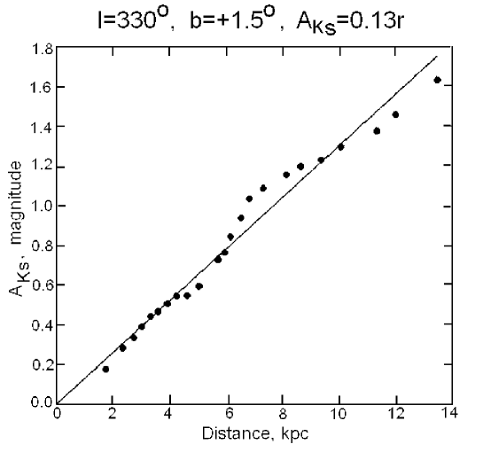
Figure 1: Example of constructing a linear fit to the law of interstellar extinction as a function of distance for a given sky region.

Figure 2: Example of identifying the red giant clump (RGC) and the red giant branch (RGB) on the color–magnitude diagram for a selected sky region.

Thus, we obtained two samples of stars: red giant branch ($\approx$1.3 million) and red clump ($\approx$10 million) stars with their photometric distances derived from Eqs. (6) and (7), respectively.

The Application of Stellar Proper Motions

We used the stellar proper motions from the Kharkiv XPM catalogue, which contains the positions and absolute proper motions of $\sim 314$ million stars. The stars cover the entire celestial sphere and have magnitudes in the range $10^{m}<B<22^{m}$. For the overwhelming majority of stars, the XPM catalogue contains their infrared $JHK$ magnitudes from the 2MASS catalogue. According to the estimate by Fedorov et al. (2011), the random errors of the XPM stellar proper motions are 3–8 and 5–10 mas yr.1 for the northern and southern skies, respectively.

The parameters of the Galactic rotation curve containing six terms of the Taylor expansion of the angular velocity of Galactic rotation $\Omega$ at the Galactocentric distance of the Sun $R_{0}=7.5$ kpc were found by Bobylev et al. (2008). Data on hydrogen clouds at tangential points (Clemens 1985), on massive star forming regions (Russeil 2003), and the velocities of young open star clusters were used for this purpose. The more recent value of R0 is $8.0\pm 0.4$ kpc (Foster and Cooper 2010). Therefore, we redetermined the parameters of the Galactic rotation curve based on the same sample but for $R_{0}=8$ kpc:

$$\begin{array}[]{lll}\Omega_{0}=-27.4\pm 0.6~{}\hbox{km s${}^{-1}$ kpc${}^{-1}$},\\ \Omega^{1}_{0}=~{}~{}3.80\pm 0.07~{}\hbox{km s${}^{-1}$ kpc${}^{-2}$},\\ \Omega^{2}_{0}=-0.650\pm 0.065~{}\hbox{km s${}^{-1}$ kpc${}^{-3}$},\\ \Omega^{3}_{0}=~{}~{}0.142\pm 0.036~{}\hbox{km s${}^{-1}$ kpc${}^{-4}$},\\ \Omega^{4}_{0}=-0.246\pm 0.034~{}\hbox{km s${}^{-1}$ kpc${}^{-5}$},\\ \Omega^{5}_{0}=~{}~{}0.109\pm 0.020~{}\hbox{km s${}^{-1}$ kpc${}^{-6}$}.\end{array}$$ (8)

The Galactic rotation curve $V_{rot}=R\Omega$ constructed with parameters (8) is shown in Fig. 3.

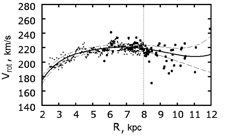
Figure 3: Galactic rotation curve (thick line) constructed with parameters (8), the dotted lines mark the 1. confidence region, the vertical line marks the Sun’s position, the black and gray circles indicate the HI and HII velocities, respectively.

Our calculations of the mean values based on a sample of distant stars showed the mean dispersion of the XPM stellar proper motions to be $\sigma_{\mu}\approx 8$ mas yr^-1 in each coordinate:

$$\begin{array}[]{lll}\overline{\mu_{\alpha}\cos\delta}=-2.1\pm 7.6~{}\hbox{ mas yr${}^{-1}$}\\ \overline{\mu_{\delta}}=-4.4\pm 7.7~{}\hbox{ mas yr${}^{-1}$}.\end{array}$$ (9)

A linear velocity of 303 km s^-1 for the distance $r=8$ kpc corresponds to $\sigma_{\mu}=8$mas yr^-1. The means (9) reflect the motion of the Sun around the Galactic center. They should be compared with the values of $\mu_{\alpha}\cos\delta=-3.151\pm 0.018$ mas yr^-1 and $\mu_{\delta}=-5.547\pm 0.026$ mas yr^-1 obtained by Reid and Brunthaler (2004) by VLBI based on an eight-year-long monitoring of the positions of the radio source Sgr A relative to two quasars. Attempts to obtain the limiting mean proper motions from the most distant stars of the XPM catalogue or only from the stars near the Galactic center direction showed that the results differ only slightly from the means (9). We may conclude that the means (9) differ from the results by Reid and Brunthaler (2004) in each of the coordinates by $\approx$ mas yr^-1. Such a difference may be related to peculiarities of the absolutization of stellar proper motions in the XPM catalogue. In spite of the fact that data on tens of thousands of extragalactic sources were used for this procedure, there were no such data near the Galactic plane. Therefore, an extrapolation procedure was applied here (Fedorov et al. 2009). On the other hand, as can be seen from Fig. 5, the mean radius of the sample of stars is about 5 kpc; therefore, the means (9) are slightly smaller than the expected values for a distance of 8 kpc.

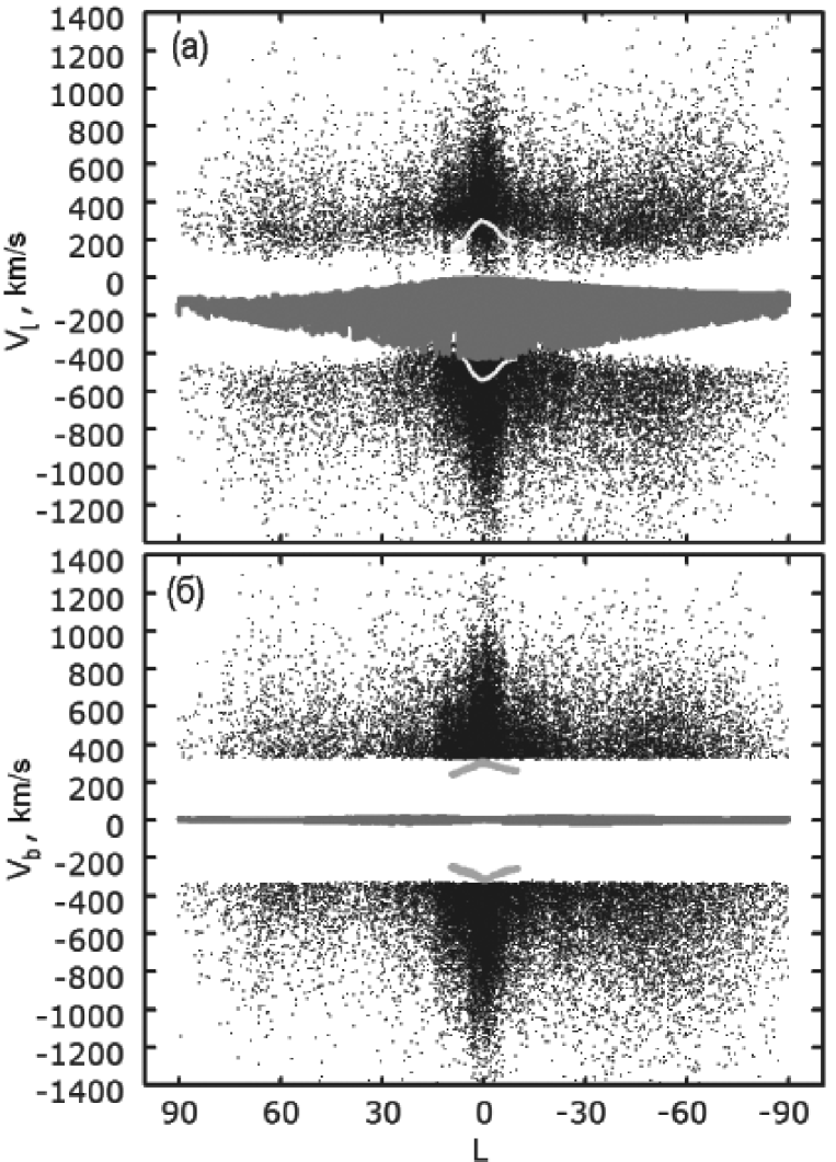
Figure 4: Velocities of red giant branch stars $V_{l}$ (a) and $V_{b}$ (b) versus Galactic longitude $l$; additional explanations are given in the text.

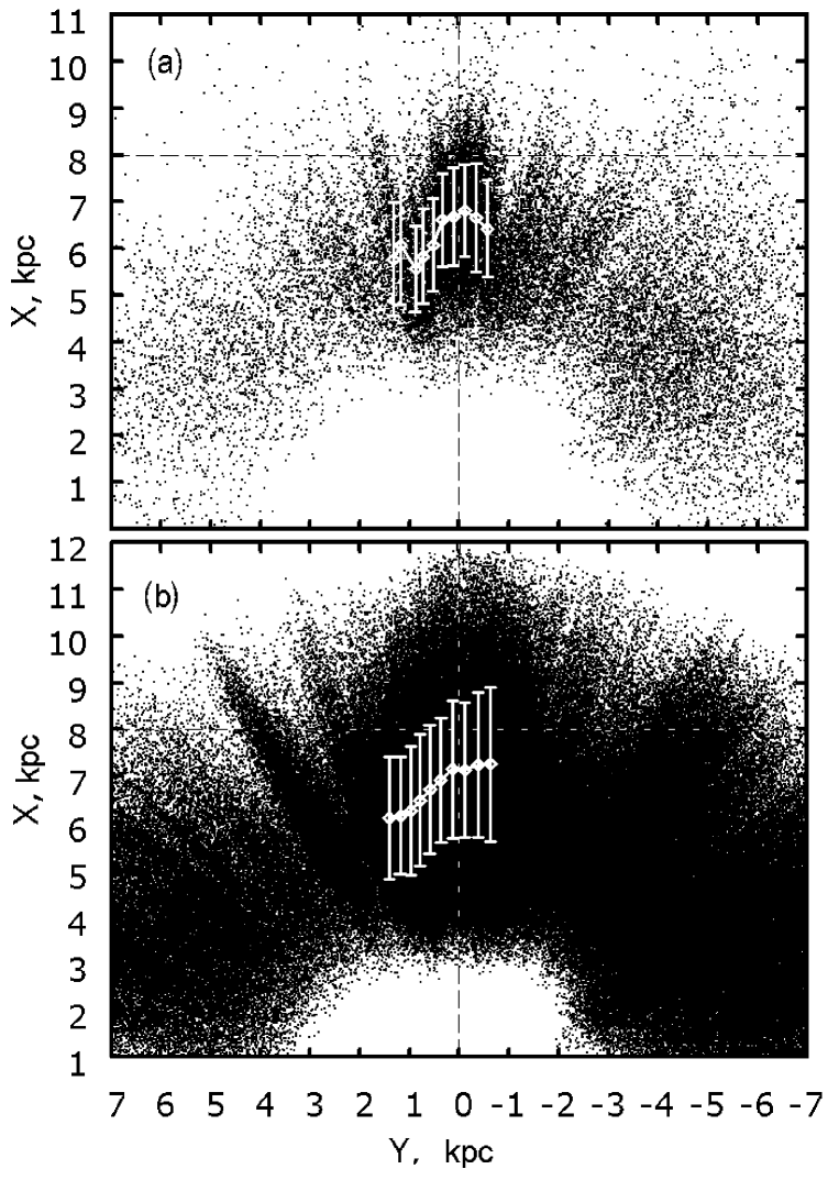
Figure 5: Distributions of red giant branch (a) and red clump (b) stars in projection onto the Galactic plane, the Sun is at the coordinate origin, the presumed Galactic center for $R_{0}=8$  kpc is located at the intersection of the dashed lines.

The application of stellar proper motions consists in the following.

(1) We take the stars close to the expected motion of the Galactic center: $|\mu_{\alpha}\cos\delta-(-3.2)|<30$ mas yr^-1 and $|\mu_{\delta}-(-5.5)|<30$ mas yr^-1, where the values from Reid and Brunthaler (2004) were taken as the means.

(2)We take the stars whose velocities deviate significantly, by $>$330  km s^-1, from the circular rotation velocity, $\approx~{}220$ km s^-1. The circular velocities are calculated from the Galactic rotation curve with parameters (8). This condition allows the stars with nearly circular orbits and foreground stars to be rejected.

(3) We use the constraint on the limiting radius of the sample r ¡ 12 kpc. The upper limit of the observed velocities for the distance $r=12$ kpc and $\sigma_{\mu}=8$ mas yr^-1 is estimated to be $4.74r3\sigma_{\mu}=1642$ km s^-1. As can be seen from Fig. 4, there are virtually no stars with such large velocities in our sample.

(4) At low Galactic latitudes, $|b|<2^{\circ}$, there is an indistinct clump of stars toward the Galactic center. The extinction is very large here and the stars of the bar are very difficult to identify. Therefore, we do not use this region. As a result, we obtained two final working samples of stars presented in Figs. 4 and 5. The corresponding plots were constructed from a sample of 45 000 red giant branch stars and 507 000 red clump stars from the range of latitudes $2^{\circ}<|b|<10^{\circ}$. The mean radius of the samples was $\overline{r}=5.1$ kpc for the red giant branch stars and $\overline{r}=5.4$ kpc for the red clump stars.

We hypothesize that the selected stars belong to the bar with a fairly high probability, although there may be some fraction of stars belonging to the bulge. Since the bulge consists mostly of fairly old stars, we believe that the percentage of bulge stars in the samples of red giant branch and red clump stars is low; therefore, it is unlikely that they can have a noticeable effect on the determination of bar characteristics.

RESULTS AND DISCUSSION

In Fig. 4, the observed velocity components for the red giant branch stars $V_{l}=4.74r\mu_{l}\cos b$ and $V_{b}=4.74r\mu_{b}$ are plotted against the Galactic longitude l. The expected velocity dispersion (their value corresponds to the $3\sigma$ level) from the model data by Zhao (1996) are marked in this figure (in the form of check marks in a direction $l\approx 0^{\circ}$); the gray shading indicates the region that the Galactic circular orbits of the stars occupy (the circular orbits for each stars were calculated with parameters (8)). It can be seen from the figure that the Galactic rotation has a significant effect when the velocities $V_{l}$ are analyzed.

Figure 5 presents the distribution of stars in projection onto the Galactic $XY$ plane. For ten directions along the line of sight, we calculated the mean coordinates and their errors. It can be seen from the figure that the part of the bar nearest to the Sun is clearly revealed by both red giant branch and red clump stars. Owing to the smaller number of stars in the sample and lesser noisiness, the distribution of red giant branch stars seems more illustrative. If we draw a line through points 3.8 (counted off from left to right) in Fig. 5a (red giant branch stars), then the bar inclination will be $35^{\circ}\pm 10^{\circ}$ to the Galactic center–Sun direction; it crosses the $OX$ axis at point $X\approx 7$ kpc, corresponding to $R_{0}=7$ kpc. In fact, however, according to present-day measurements, $R_{0}=8.0$ kpc. If we draw a line through points 3–4 and $X=8$ kpc, then the inclination of the bar axis will be $21^{\circ}\pm 10^{\circ}$. Analysis of the distribution of red clump stars (Fig. 5b) also yields similar results, but, as can be seen from Fig. 5b, the mean values are calculated from them with errors larger than those from red giant branch stars by a factor of 1.5.

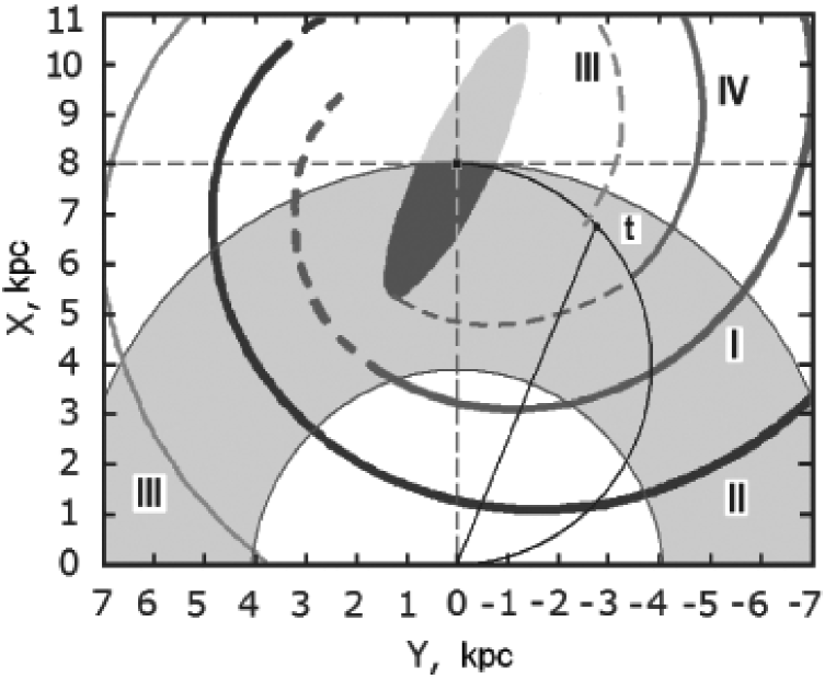
Figure 6: Proposed model of the bar and refined (in the inner Galaxy) model of a four-armed spiral pattern for the Galaxy, the gray shading in the region 4 kpc $<r<$ 8 kpc indicates the model distribution of stars, the light shading indicates the far, unobserved end of the bar, the dark shading marks the observed region of the bar; for additional explanations, see the text.

In addition to the bar, the velocity peaks in Fig. 4 and the star density maxima in Fig. 5 also reflect the spiral structure of the Galaxy. An asymmetry is clearly seen in the distribution of stars in Fig. 5, where there are much more stars in the right part of the figure. The influence of the Carina–Sagittarius arm is In addition to the bar, the velocity peaks in Fig. 4 and the star density maxima in Fig. 5 also reflect the spiral structure of the Galaxy. An asymmetry is clearly seen in the distribution of stars in Fig. 5, where there are much more stars in the right part of the figure. The influence of the Carina–Sagittarius arm is clearly reflected in a direction $l\approx-15^{\circ}$, with this influence being more tangible in the negative velocities $V_{l}$ (Fig. 4).

The solid lines in Fig. 6 indicate the four-armed spiral pattern with the pitch angle $i=13^{\circ}$ constructed from the data by Bobylev and Bajkova (2013), in which the pattern parameters were obtained by analyzing the distribution of maser sources with measured trigonometric parallaxes in the Galaxy. The designations of the spiral arms are as follows: I – Scutum–Crux arm, II – Carina–Sagittarius arm, III – Perseus arm, IV – Outer arm (or Cygnus arm). The dashes indicate the extensions of the spiral arms that, in our opinion, correspond more closely to the available data. The thin black line indicates a semicircumference with the radius $R_{0}/2=4$ kpc; the center of this circumference lies on the Sun.Galactic center line. Such a circumference is the locus of tangential points, the points where the circular rotation velocity of the Galaxy lies exactly along the line of sight. Point $t$ seen in the direction $l=-22^{\circ}$ is marked on the semicircumference. According to radio-astronomical observations of the HI line-of-sight velocities, it is in this direction that the 3-kpc spiral arm is observed tangentially (Burton 1988). The distance from the Galactic center to point t is 3 kpc (hence the name of this arm). The figure shows the bar with a radius of 3 kpc oriented at an angle of 25. to the Galactic center.Sun direction. The near end of the bar is seen at the angle $l=10^{\circ},$ which well reflects our map of the distribution of stars (Fig. 5) and the counts by Rattenbury et al. (2007).

The proposed scheme (Fig. 6) agrees well with the cartographic model of a four-armed spiral pattern by Vall$\acute{e}$e (2008) and the conclusion about the number of arms in the Galaxy reached by Efremov (2011) by analyzing the large-scale distribution of neutral, molecular, and ionized hydrogen clouds in the Galaxy.

Note that the spikes in $V_{l}$ and $V_{b}$ are observed when the line of sight runs along the spiral arm. Note the significant clump of stars in the left part of Fig. 5 at $l=12^{\circ}$, which is confirmed by the corresponding narrow peak in the velocity distribution in Fig. 4. The stars in this direction are slightly farther from the bar end (points 1.2); a similar zigzag at $l=10^{\circ}$ is also seen in the estimates by Rattenbury et al. (2007). This can be explained if the spiral arms form something in the form of a ring or oval elongated along the major axis of the bar. The line of sight will then run along this structure.

To better understand the situation in the immediate vicinity of the bar, we performed Monte Carlo simulations. The results are presented in Fig. 7. Figure 7a shows a map of the distribution of stars corresponding to the model presented in Fig. 6. In the range of distances $4<r<8$ kpc and in the spiral arm segments, the stars were distributed uniformly randomly; in the bar, they were distributed normally (we use only the near part of the bar, because we do not see the far one). The sample consisted of 35 000 stars (brought closer to the sample of red giant branch stars). One Monte Carlo realization obtained for model errors in the stellar distances of 10% is presented. Figure 7b shows a map of the distribution of stars where a ring with a radius of 2 kpc fringing the bar was added to the preceding model.

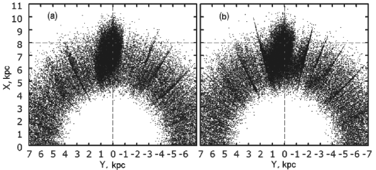
Figure 7: Monte Carlo realization of the model presented in Fig. 6a, Monte Carlo realization of the complicated model with the addition of a ring 2 kpc in radius centered at the Galactic center; for additional explanations, see the text.

Our simulations lead us to several conclusions. (1) Although the bar in the model is oriented at an angle of 25^∘ to the Galactic center – Sun direction, the ellipse of the apparent (smeared by the distance errors) distribution of stars is oriented at a smaller angle of about 15^∘. (2) In spite of the fact that we used rather narrow spiral arms, our model data (Fig. 7) well approximate the actually observed ones (Fig. 5). (3) The model with a ring (Fig. 7b) provides a more accurate approximation.

CONCLUSIONS

We proposed and implemented a method for selecting stars belonging to the Galactic bar. This method is based on 2MASS infrared photometry and stellar proper motions, in particular, from the Kharkiv XPM catalogue. It consists in the following: (1) the pre-selection of red clump and red giant branch stars on the color–magnitude diagram for which the photometric distances are determined; (2) the elimination of background stars from the preselected samples using constraints on the proper motions, because the stellar proper motions are indicators of a larger velocity dispersion toward the bar and the spiral arms compared to the background stars. By the background we mean the stars with circular orbits.

As a result, we obtained two samples of stars, 45 000 red giant branch stars and 507 000 red clump stars from the range of latitudes $2^{\circ}<|b|<10^{\circ}$ at longitudes $|l|<90^{\circ}$, based on which we mapped the distribution in the Galactic XY plane.

Analysis of the maps allowed the bar segment nearest to the Sun with an orientation of 20^∘–25^∘ with respect to the Galactic bar – Sun direction and a semimajor axis of no more than 3 kpc (short bar) to be identified with confidence.

Our numerical simulations of the velocities and distribution of stars allowed the model of a four-armed spiral structure of the Galaxy in the immediate vicinity of the bar to be refined. In particular, we found arguments for the fact that an extension of the Perseus arm(III) is the 3-kpc arm segment and that the Outer arm (IV) begins from the bar end nearest to the Sun. It is quite likely that all spiral arms merge into a 3-kpc oval (an ellipse or ring). In fact, this may imply that two spiral arms can emerge from each end of the bar.

REFERENCES

1. C. Babusiaux and G. Gilmore, Mon. Not. R. Astron. Soc. 358, 1309 (2005).
2. R. A. Benjamin, E. Churchwell, B. L. Babler, et al., Astrophys. J. 630, L149 (2005).
3. J. Binney, O. E. Gerhard, A. A. Stark, et al., Mon. Not. R. Astron. Soc. 252, 210 (1991).
4. L. Blitz and D. N. Spergel, Astrophys. J. 379, 631 (1991).
5. V. V. Bobylev, A. T. Bajkova, and A. S. Stepanishchev, Astron. Lett. 34, 515 (2008).
6. V. V. Bobylev and A. T. Bajkova, Astron. Lett. 39, 809 (2013).
7. W. B. Burton, Galactic and Extragalactic Radio Astronomy, Ed. by G. Verschuur and K. Kellerman (Springer, New York, 1988).
8. D. P. Clemens, Astrophys. J. 295, 422 (1985).
9. T. M. Dame and P. Thaddeus, Astron. J. 683, L143 (2008).
10. B. T. Draine, Ann. Rev. Astron. Astrophys. 41, 241 (2003).
11. Yu. N. Efremov, Astron.Rep. 55, 108 (2011).
12. P. Englmaier, M. Pohl, and N. Bissantz, Mem. Soc. Astron. Ital. 18, 199 (2011).
13. P. N. Fedorov, A. A. Myznikov, and V. S. Akhmetov, Mon. Not. R. Astron. Soc. 393, 133 (2009).
14. P. N. Fedorov, V. S. Akhmetov, V. V. Bobylev, and G. A. Gontcharov, Mon. Not. R. Astron. Soc. 415, 665 (2011).
15. T. Foster and B. Cooper, ASP Conf. Ser. 438, 16 (2010).
16. C. Francis and E. Anderson, Mon. Not. R. Astron. Soc. 422, 1283 (2012).
17. G. A. Gontcharov, Astron. Lett. 37, 785 (2008).
18. G. A. Gontcharov, Astron. Lett. 37, 707 (2011).
19. E. Hog, C. Fabricius, V. V. Makarov, et al., Astron. Astrophys. 355, L27 (2000).
20. L. G. Hou, J. L. Han, and W. B. Shi, Astron. Astrophys. 499, 473 (2009).
21. J. R. D. Lpine, Yu. N. Mishurov, and S. Yu.Dedikov, Astrophys. J. 546, 234 (2001).
22. M. Lpez-Corredoira, A. Cabrera-Lavers, T. J. Mahoney, et al., Astron. J. 133, 154 (2007).
23. D. J. Marshall, A. C. Robin, C. Reyle, et al., Astron. Astrophys. 453, 635 (2006).
24. A. M. Mel’nik and P. Rautiainen, Astron. Lett. 35, 609 (2009).
25. Y. Nakada, T.Onaka, I. Yamamura, et al., Nature 353, 140 (1991).
26. D. M. Nataf, A. Gould, P. Fouqu, et al., Astrophys. J. 769, 88 (2013).
27. N. J. Rattenbury, S. Mao, T. Sumi, et al., Mon. Not. R. Astron. Soc. 378, 1064 (2007).
28. M. Reid and A. Brunthaler, Astrophys. J. 616, 872 (2004).
29. D. Russeil, Astron. Astrophys. 397, 133 (2003).
30. A. Sanna,M. J. Reid, L. Moscadelli, et al., Astrophys. J. 706, 464 (2009).
31. M. F. Skrutskie, R. M. Cutri, R. Stiening, et al., Astron. J. 131, 1163 (2006).
32. K.Z.Stanek,M.Mateo, A. Udalski, et al.,Astrophys. J. 429, L73 (1994).
33. A. Udalski, M. Szymanski, K. Z. Stanek, et al., Acta Astron. 44, 165 (1994).
34. J. P. Valle, Astron. J. 135, 1301 (2008).
35. G. de Vaucouleurs, in The Spiral Structure of Our Galaxy, Ed. W. Becker and G. Contopoulos (Reidel, Dordrecht, 1970), p. 18.
36. Y.Wang,H. Zhao, and S. Mao,Mon. Not.R. Astron. Soc. 427, 1429 (2012).
37. H. Zhao,Mon. Not. R. Astron. Soc. 283, 149 (1996).