Bright Blazhko RRab Lyrae stars observed by ASAS and the SuperWASP surveys

Abstract

Aims. Period study of 321 fundamental mode RR Lyrae type stars (RRab), which had appropriate data in ASAS and SuperWASP surveys, was performed to complement and extend the list of known Blazhko stars in galactic field with bright stars up to 12.5 mag in maximum light.

Methods. An individual approach was applied to each studied star. Permanent visual supervision was maintained to each procedure in data analysis (data cleaning, frequency spectra examination) to avoid missing any possible sign of the Blazhko effect. Period analysis was performed using Period04 software.

Results. We found 100 stars to be definitely modulated. In 25 cases, previously unknown modulation was revealed and 8 new candidates for Blazhko stars were identified. Their modulation needs to be confirmed. In 18 previously found Blazhko stars, no modulation was detectable. Multiple modulation was revealed for eight stars that were previously proposed to show simple modulation. In total, there were twelve stars with some peculiarity in their modulation in the sample. This brings the incidence rate of multiple/irregularly-modulated stars to 12 %. The ratio of the modulation periods of five of the double-modulated stars was within the ratios of small integers. One of stars studied, IK Hya, showed a very interesting frequency spectrum, which we interpret as changing Blazhko period between 71.81 and 75.57 days and an additional 1403-day-long cycle analogous to a four-year cycle of the prototype RR Lyr. The limits of the shorter period produce a beating period that is approximately twice as big as a 1403-day period. The newly revealed Blazhko star RZ CVn seems to undergo changes in the amplitude of the modulation, as well as in the basic pulsation and Blazhko periods. We found that the incidence rate of the Blazhko RR Lyraes is at least 31 %, more likely even higher. It was also found that the majority of the Blazhko variables show triplet structures in their frequency spectra and that in 89 % of these cases, the peak with larger amplitude is on the right-hand side of the main pulsation component.

1 Introduction

Data from automatic sky surveys provide an invaluable opportunity for finding new variables and for long-term monitoring of the sky. The most extensive survey of Galactic field variable star research are without doubt Polish ASAS (All Sky Automated Survey; see e.g. Pojmanski 1997, 2002) and SuperWASP (Super Wide Angle Search for Planets, hereafter SW; Pollacco et al. 2006; Butters et al. 2010) managed by the University of Leicester. Both projects have been run for several years.

Field RR Lyraes have been studied many times on the basis of various sky surveys. Among others, Kinemuchi et al. (2006) and Wils et al. (2006) utilized data from Northern sky variability survey (NSVS, Woźniak et al. 2004), e.g. Kovács (2005), Szczygieł et al. (2009) studied RR Lyraes based on ASAS data, and Drake et al. (2013) dealt with RR Lyraes measured in Catalina sky survey. Probably the most precise ground-based survey data were provided by the Konkoly Blazhko survey, which have been operated since 2004 (e.g. Jurcsik at al. 2009a; Sódor 2007; Sódor et al. 2012).

Crucial advances in Blazhko effect research have been made recently by space missions CoRoT and Kepler. Ultra-precise data provided by these space telescopes allowed findings of, say, cycle-to-cycle variations now known as period doubling (Szabó et al. 2010; Kolenberg et al. 2010; Benkő et al. 2010) or long-term changes in the Blazhko effect and excitation of additional modes (Poretti et al. 2010; Chadid et al. 2010; Guggenberger et al. 2012).

Large samples of Blazhko RR Lyrae stars in galactic bulge were also studied in the framework of MACHO and OGLE surveys (Soszyński et al. 2011; Moskalik & Poretti 2003). Since the stars in the bulge are faint and are not included in ASAS or SW surveys, we did not deal with them.

Special papers based on ASAS data, which are at least partially devoted to Blazhko stars in our Galaxy, were published by Kovács (2005), Wils & Sódor (2005) (hereafter WS05), and Szczygieł & Fabrycky (2007) (hereafter SF07), who all revealed many new Blazhko variables and gave a list of them. An extensive study of the Blazhko effect is presented in the paper of Le Borgne et al. (2012), which is based on observations made with TAROT telescopes (Klotz et al. 2008, 2009). Le Borgne et al. (2012) also made use of $O-C$ information stored in the GEOS RR Lyr database (Le Borgne et al. 2007) and gave a list of galactic field Blazhko stars. A regularly updated database of known Blazhko RR Lyraes situated in the galactic field (BlaSGalF, Skarka 2013) recently contained about 270 objects.

There are a few studies of particular RR Lyraes proceeded from SW mesurements, e.g. the TV Boo study made by Skarka & Zejda (2013), or Srdoc & Bernhard (2012), who revealed the Blazhko effect in GSC02626-00896, but a comprehensive study of RR Lyraes based on SW data has not been performed yet.

RR Lyraes with appropriate ASAS and SW data were in the spotlight. The goal was to search for the presence of the Blazhko modulation and to describe its characteristics (pulsation and modulation periods and multiplicity/irregularity of the modulation). We applied commonly used techniques of light curve and frequency spectra examination to complement and extend the list of known Blazhko stars with bright RR Lyraes (up to 12.5 mag in maximum light). To be as precise as possible, we carefully cleaned and analysed each light curve and frequency spectra individually.

2 The data

2.1 Data characteristics

Both ASAS and SW data are products of measurements with low-aperture telescopes. ASAS uses Johnsons $V$ and $I$ filters, while SW telescopes are equipped with a broad-band filter (from 400 to 700 nm) (Pojmański 2001; Pollacco et al. 2006). The typical scatter of points is difficult to define, because it changes from target to target. In the case of ASAS it is from about 0.02 to 0.1 mag, while SW scatter extends from 0.007 to 0.04 mag for our sample stars. Also the time span and the distribution of the data differ for both surveys and various targets.

ASAS data typically cover a few years (up to year 2009) with point-to-point spacing between two and four days with only small gaps between observational seasons. Typical sampling of SW data points is between five and twelve minutes. Therefore SW data are generally more numerous and more dense than ASAS data, but they typically span only one or two seasons (see last columns in Tables 1-5). These characteristics resulted in a typical Nyquist frequency from 0.17 to a few tens for ASAS and in 100 to more than 1000 c/d in the case of SW. For differences between ASAS and SW data see fig. 1, where data for RY Col are plotted with their spectral windows.

Figure 1: Differences between ASAS (left column) and SW (right column) data of RY Col together with their spectral windows (bottom panels). ASAS data are more or less uniformly distributed, while SW data show a large gap between observing seasons. Both spectral windows are dominated by strong daily aliases. Except these, SW data suffer from additional artefacts, namely from yearly aliases.

2.2 Sample selection and data cleaning

The basic set of the stars originated in the GCVS catalog (Samus et al. 2012), which contains 512 stars of RRab type brighter than 12.5 mag in maximum. This magnitude limit was chosen to analyse only stars with the best data quality – the scattering of data points over 13 mag rapidly increases. The list extracted from GCVS was completed with 82 stars, which did not have a GCVS designation in 2012 and which were taken from SF07 and Szczygieł et al. (2009). There were data for 475 stars available in the ASAS database, and for 243 RR Lyrae stars in the SW archive. Data of 161 stars appeared in both the ASAS and SW archives. This means that a total of 557 stars remained for further analysis.

Unfortunately, data from automatic surveys are often very noisy and of bad quality. Therefore we first looked for ephemeris of the stars in the Variable star index, VSX (Watson et al. 2006) to be able to construct phased light curves. This was done to quickly check the quality of the data. In many cases, the periods that we found were not current. Therefore we were forced to update and roughly estimate the actual pulsation period. For this purpose, as for all our other period analyses, Period04 software (Lenz & Breger 2004) was used.

In the case of ASAS survey, only the best quality $V$-data (with flags A and B) were used. Following Kovács (2005), ASAS $V$ magnitude was calculated as the weighted average of five values in different apertures using

$$V(t)=\frac{\sum^{5}_{i=1}V_{i}\left(t\right)\sigma^{-2}_{i}\left(t\right)}{\sum^{5}_{i=1}\sigma^{-2}_{i}\left(t\right)}.$$ (1)

Only light curves with more than 200 points from ASAS and with more than 1000 points from SW were left in the sample for further investigation.

Once the phased light curves were prepared, we briefly surveyed them to immediately discard stars whose data, at a glance, were very noisy. Remaining light curves were then fitted with the sum of sines and points that were farther away than 0.5 mag from the fit were automatically removed. This procedure guaranteed that real outliers were eliminated and points scattered by a possible Blazhko effect remained in the dataset. A careful visual examination of all light curves was then applied, and points, which were unambiguously caused by noise, were manually deleted. In the case of SW stars, we also visually scanned time series night-by-night and removed outliers, as well as entire noisy nights. Figure 2 shows steps in the cleaning process in the case of V559 Hya.

SW data often contained vertically shifted multiple points. This was the consequence of simultaneous imaging of the target by a few cameras. To avoid using such data, the information about the position of the star on the chip (fig. 3 bottom panels) was utilized. If the separation of the data from two cameras was impossible, each star with a vertical separation of points larger than 0.01 mag was discarded. This was the case, for instance, for DM And (fig. 3), which shows previously unknown modulation.

Several targets from SW underwent vertical shifts of points taken in different seasons (as the third season of DM Cyg, fig. 3). If so, seasons were phased separately, and the light curves were fitted with the sum of sines to get zero points. Afterwards, the points from different seasons were shifted to fit one each other. This procedure was used in the case of U Tri, among others, and magnitudes of the first part of the dataset were decreased by 0.09 mag. In some cases, vertical shifts were present even in one season. In such cases, we removed the whole season from the dataset. If all seasons underwent shifts, the star was discarded from our sample. Only 321 variables met all the above-mentioned criteria and were accepted for further analysis.

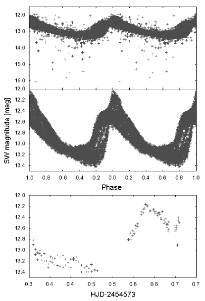
Figure 2: Steps in the cleaning process in V559 Hya. There are raw SW data folded with the main pulsation period taken from VSX on the top panel. The middle panel shows phased data after cleaning process. The bottom panel is a sample of one of omitted nights, which was discarded due to poor quality of the data.

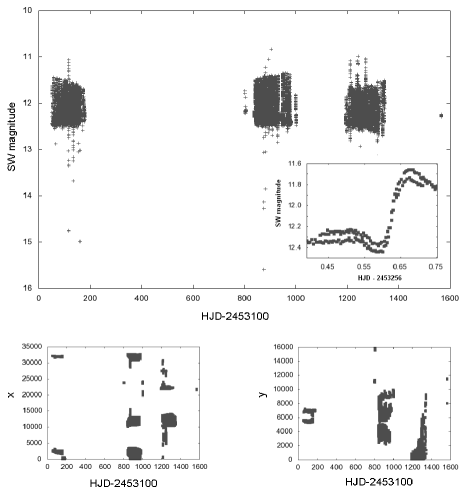
Figure 3: Illustration of difficulties in SW data processing on the case of DM And. The upper panel shows raw data. The change in amplitude of this star caused by the Blazko effect is apparent. The detail shows the night HJD 2453256, where the vertical shift between data coming from various cameras is demonstrated. The distribution of the positions of the star on the chip in x and y directions during the whole observation period are shown in the bottom part of this figure.

3 Light curve and frequency spectra examination – looking for the Blazhko effect

3.1 Introductory remarks on the Blazhko effect

The manifestations of the Blazhko effect, which is usually defined as phase and/or amplitude modulation of the light curve with periods between a few days and several thousand days, can be very heterogeneous and in many cases are difficult to uncover. The most conspicuous feature of the Blazhko effect is the change in amplitude of the light variations, which can be more than 0.5 mag (e.g. XY Eri or IK Hya, Le Borgne et al. 2012), but also less than a tenth of a magnitude (e.g. DM Cyg, Jurcsik et al. 2009b) or even only a few hundredths of magnitude – KIC 11125706 with the amplitude of the modulation of only 0.015 mag (Benkő et al. 2010). The same applies to the range of phase variations – in RR Gem the Blazhko effect causes scarcely perceptible changes in $O-C$ of 0.004 d (Le Borgne et al. 2012), while some stars change their $O-C$s in more than 0.07 d (e.g. XY Eri, V445 Lyr ($\Delta O-C=0.15$ d) Le Borgne et al. 2012; Guggenberger et al. 2012).

When analysing the frequency spectra of Blazhko stars, we can expect characteristic structures to be present. Firstly, the Blazhko effect manifests itself as an additional peak $f_{\mathrm{BL}}$ in the range of $\sim$0.0001 to 0.2 cycles per day. But, the most prominent features of Blazhko-frequency spectra are characteristic series of equidistant peaks around basic pulsation frequency and its harmonics ($kf_{0}\pm lf_{\mathrm{BL}}$, where $f_{0}$ is the basic pulsation frequency and $k$ and $l$ are integers) with rapidly decreasing amplitudes. In data with limited precision, multiplets can be strongly reduced by noise and only the highest peaks are found. In such a case, we observe only triplets or even doublets. In contrast to limited ground-base observations, in data gathered from space, high-order multiplets are observed (e.g. in V1127 Aql, where sepdecaplets ($l=8$) were identified Chadid et al. 2010).

Multiplets must not be strictly equidistant and side peaks do not have to have the same amplitude – it depends on many factors, mainly on the mixture of amplitude and frequency modulation (for more details see Benkő et al. 2011). In addition, recent studies have shown that the Blazhko effect can be multiple (e.g. like CZ Lac Sódor et al. 2011), a very irregular and complex phenomenon affected by long-term and/or sudden changes, as in RR Lyrae itself, where a four-year long cycle was found, during which pulsation and modulation characteristics are changing (Detre & Szeidl 1973; Kolenberg et al. 2011b; Stellingwerf et al. 2013). During this long cycle, the Blazhko effect can almost disappear.

Another examples of complexity of modulation show CoRoT 105288363 and V445 Lyr, which seem to undergo drastic changes in their Blazhko effect (Guggenberger et al. 2011, 2012). Changing Blazhko modulations like these, especially strong ones like in V445 Lyr, will lead to a different frequency pattern with more peaks than the normal multiplet. There will be additional peaks or even additional multiplets in cases with an irregular or changing modulation.

All these illustrations demonstrate the variety and complexity of the Blazhko effect. Especially when analysing data from ground-base automated surveys, one should be very careful when identifying the Blazhko effect and interpreting the frequency spectra. It is very difficult to distinguish between long-term Blazhko modulation, period changes and multiple or irregular modulation, because all these processes produce additional peaks close to the basic pulsation components. If the data are of bad quality or are badly distributed or if the observations are not sufficiently spread out in time, the presence of the Blazhko effect in frequency spectra could even stay hidden.

Although astronomers have known about the existence of the Blazhko effect since the beginning of the 20th century and much progress have been made (e.g. revealing period doubling by Szabó et al. 2010), a suitable physical explanation is still not available. For more information about the Blazhko effect and proposed models in general see e.g. Kovács (2009), Kolenberg (2011a), and references therein.

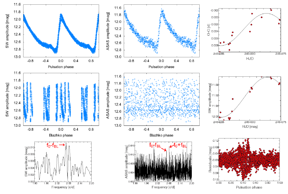
Figure 4: Analysis of HH Tel. First column shows cleaned SW data folded according to epoch 2454347.2643 with the main pulsation period $P=0.4820925$ d (top panel) and with the Blazhko period 133 d (middle panel). Frequency spectrum based on SW data in the vicinity of $f_{0}$ prewhitened with $kf_{0}$ is shown in the bottom panel in the first column. Second column displays the same as the first one but for the ASAS data. In the third column (based on SW data again), there are from the top changes in $O-C$ values, changes of maximum brightness, and residuals after prewhitening with the main pulsation components at the bottom (epoch is shifted of a half of a period for better arrangement). For details see the text in section 3.2.

3.2 Methods of searching for the Blazhko effect

Searching for the Blazhko effect actually started during the cleaning process when phased light curves were examined. High-amplitude modulation was easily resolvable by a fleeting glance at the data. Our methods, inspired by methods used e.g. in Alcock et al. (2003), WS05, and Le Borgne et al. (2012), can be summarized in four points:

1. Phased light curve visual examination – visual inspection of the phased light curve to reveal a characteristic scattering around maximum light.

2. Frequency spectra analysis with Period04 – frequencies were fitted independently; i.e., we scanned for frequencies with the highest amplitude and subsequently subtracted them. This was done in the range of $0-30$ c/d down to the signal-to-noise ratio $(S/N)$ of the peaks higher than four. We searched for the manifestation of the Blazhko effect in the vicinity of the main pulsation components, as well as for the presence of the Blazhko peak itself (in the range of $\sim$0.0001 to 0.2 c/d). All uncertainties were estimated using Period04 tools.

3. Checking of residuals – In stars with only basic pulsation components in frequency spectrum, residuals after prewhitening were visually inspected to see whether there were any typical inhomogeneities possibly caused by the Blazhko effect.

4. Magnitude-at-the-maximum-light vs. time-of-the-maximum series analysis – this was done only for the SW sample, because ASAS light curves, with few exceptions, did not contain continuous time series to determine times and magnitudes of the maximums. For $Mag_{\mathrm{max}}$ and $T_{\mathrm{max}}$ determination, low-degree polynomial fitting (typically up to 5th order) was used. Only well defined maximums were fitted. In the next step, frequency analysis of such a series was performed to search for significant peak in the range of $\sim$0.0001 to 0.2 c/d.

Each star was analysed on an individual basis without any automatic procedures (except outliers removing and prewhitening of the frequency spectra). We maintained permanent visual supervision of all steps to avoid omitting any possible sign of the Blazhko effect. A candidate was marked as a Blazhko star only if we were able to find the modulation period or if there was no doubt about the Blazhko effect. Some exceptions, e.g. LS Boo, are discussed in sects. 4.3 and 5.1.

As an example of the procedures used, the analysis of HH Tel (fig. 4) is demonstrated. This star was revealed to be a new Blazhko star. Data from both surveys are plotted at the top in the first two columns of fig. 4. We can see a weak sign of the modulation around maximum light (especially in SW data). This indicated that the Blazhko effect might be present. Frequency spectra analysis down to $S/N=4$ unveiled only the main pulsation components. After prewhitening peaks that could possibly be caused by the Blazhko effect ($f_{0}\pm f_{\mathrm{Bl}}$) were identified, but they are of very low amplitude with $S/N\sim 3$ (fig. 4 two left bottom panels). No distinct peak in the range of $\sim$0.0001 to 0.2 c/d was noted.

Therefore, searching for additional peaks in the frequency spectra of the light curve had ambiguous success. But the SW residuals (right bottom corner of fig. 4) showed a tell-tale characteristic of the Blazhko effect: typically scattered points around the position corresponding to ascending branch and maximum light.

The last step was to determine the modulation period. For this purpose, the times ($T_{\mathrm{max}}$) and brightnesses of maximum light ($Mag_{\mathrm{max}}$) were used. Period analysis of such data directly revealed a modulation period of 133(9) d, while weak peaks identified in Fourier spectra of the light curves gave values 143(1) d and 123(5) d for ASAS and SW data, respectively. All values are very inaccurate, which is due to the limited time scale of SW data (only one Blazhko cycle) and due to the imprecision of ASAS data.

At that stage we were able to construct Blazhko phased light curves (first two columns in the middle of fig. 4) to check for the correctness of the value we found. SW data showed a typical ‘Blazhko’light curve, while there was no sign of modulation in the ASAS Blazhko light curve.

HH Tel was chosen intentionally to show that it is very problematic to decide the Blazhko nature of this star based on ASAS data alone, while there is no doubt about the modulation in SW data. The example of HH Tel clearly shows that many unveiled Blazhko stars could remain in the ASAS database.

4 Blazhko stars from ASAS

4.1 Known Blazhko stars

A review of 62 previously known Blazhko stars contained in our ASAS sample is given in Table 1. For comparison the values of Blazhko periods found by WS05 and SF07 are also given (5th and 6th column). These are naturally very similar to ours, because we studied the same, but more extended data. Therefore, with respect to periods, only a revision of the ASAS data was actually performed.

Epochs given in Table 1 are not times of maxima, which are usually given, but they are arbitrarily chosen to obtain Blazhko-phased light curves, as well as the light curves phased with the main pulsation period, with the maximum around the zero phase. The amplitudes $A_{+}$, $A_{-}$ of the side peaks $f_{\pm}=f_{0}\pm f_{\mathrm{BL}}$ corresponding to the Blazhko period $P_{\mathrm{BL}}$ are in 7th and 8th columns and their ratio ($A_{+}/A_{-}$) in 9th column, respectively. All given Blazhko periods in the study correspond to the side peak with the highest amplitude in frequency spectrum. Label ‘$n$’denotes the number of points used and ‘$TS$’their time span.

Eight of these stars (marked by an asterisk) showed additional peaks close to the basic pulsation components, which could possibly point to irregularity in modulation, period changes, or multiplicity of a modulation. The modulation periods for VX Aps, GS Hya, and AS Vir were estimated for the first time. The only equally spaced quintuplet was identified in RS Oct (fig. 5).

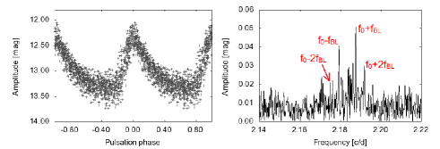
Figure 5: RS Oct – the only star in our ASAS sample, which showed equally spaced quintuplet.

Table 1: Known Blazhko stars from our ASAS sample

Star	Epoch HJD	$P_{\mathrm{puls}}$ [d]	$P_{\mathrm{BL}}$ [d]	WS05	SF07	$A_{-}$ [mag]	$A_{+}$ [mag]	$A_{+}/A_{-}$	$n$	$TS$ [d]
BS Aps	2454527.8757	0.5825596(7)	46.53(7)			-	0.026	-	646	3210
VX Aps	2451981.7844	0.484663(2)	171.8(6)			0.024	0.039	1.60	647	3210
TY Aps	2452088.5376	0.501698(1)	108.6(2)			0.033	0.049	1.48	601	3208
V360 Aqr	2452168.6700	0.626946(3)	54.44(4)		54.52	-	0.097	-	413	3254
S Ara *	2454247.7025	0.451849(1)	49.51(5)	49.5	49.37	0.043	0.044	1.02	507	3175
TT Cnc	2454202.5461	0.563454(1)	88.8(2)			0.022	0.045	2.05	342	2546
RV Cap	2452002.1370	0.4477426(6)	232.3(5)		231.66	-	0.105	-	543	3117
Star 1	2452034.5590	0.526235(1)	694(10)		666.44	0.037	0.065	1.78	509	3245
BI Cen	2454932.6911	0.4531949(4)	79.45(9)		79.01	0.039	0.042	1.08	767	3179
RX Cet	2454666.8472	0.573741(1)	261.5(8)	256	255.5	0.058	-	-	397	3287
RV Cet	2452080.9219	0.6234136(8)	112.0(1)	112	112.05	0.025	0.040	1.60	394	3275
RX Col	2454751.8312	0.593749(3)	132.5(4)	130		-	0.043	-	675	3298
RY Col	2453854.5121	0.4788357(5)	82.12(7)	82	81.95	0.028	0.073	2.61	624	3298
WW CrA	2452514.1932	0.559490(1)	35.69(2)	35.5		0.039	0.025	0.64	530	3176
V413 CrA	2454508.8898	0.5893427(4)	60.5(2)		59.96	0.009	0.010	1.11	542	3158
X Crt	2453449.7158	0.732836(1)	143.8(3)	143		-	0.017	-	436	3296
VW Dor *	2454136.7779	0.5705770(7)	25.92(2)	25.9		0.014	-	-	667	3295
XY Eri	2452553.7594	0.554250(1)	50.11(5)	50		0.052	0.079	1.52	511	3287
LR Eri *	2453408.6223	0.602228(1)	123.5(6)	122		-	0.045	-	893	3296
Star 2	2453745.5476	0.62963274(9)	330(2)		335.29	0.033	0.050	1.51	683	3296
RX For	2452082.9124	0.5973129(8)	31.80(6)	31.8	31.81	-	0.061	-	517	3287
SS For	2451869.5957	0.4954329(4)	34.84(1)	34.8	34.88	0.026	0.064	2.51	501	3295
RT Gru	2452858.6870	0.512169(1)	86.94(8)			-	0.079	-	496	3256
DL Her	2453477.7851	0.591631(1)	34.66(4)			-	0.038	-	427	2396
BD Her	2453496.8160	0.473794(1)	21.68(1)			0.052	0.085	1.63	308	2417
GS Hya	2451998.7258	0.522829(1)	42.8(5)			0.051	-	-	453	3186
UU Hya	2453761.7195	0.5238652(9)	39.93(4)			0.042	-	-	349	3112
SV Hya	2452062.5225	0.4785476(3)	63.23(4)	63	63.29	0.022	0.028	1.27	877	3178
V552 Hya	2454931.6746	0.3987697(8)	48.53(3)	48.3		0.142	0.072	0.51	443	3177
V559 Hya *	2454199.5359	0.447944(2)	26.469(6)	26.6	26.5	0.076	0.135	1.78	454	3187
SZ Hya	2454258.5213	0.537225(1)	26.26(2)	26.3	26.3	0.076	0.080	1.05	543	3298
DD Hya	2454408.8593	0.5017706(6)	34.44(4)			0.036	0.027	0.75	634	3142
SZ Leo	2455012.4827	0.534080(9)	177.8(7)	179		0.091	0.062	0.61	339	2560
BB Lep	2452128.9235	0.5389127(9)	22.86(1)		22.84	0.039	0.041	1.05	567	3300
MR Lib	2453133.7052	0.540065(1)	41.85(3)	41.7	41.77	0.051	0.115	2.25	430	3172
PQ Lup	2453861.6802	0.581994(1)	48.77(3)	48.8	48.82	-	0.068	-	478	3189
V339 Lup	2453897.6107	0.6005772(7)	49.7(9)	49.5		0.014	0.029	2.07	526	3191
Star 3	2453428.6223	0.5501319(9)	37.2(2)		37	0.046	0.059	1.28	466	3186
UV Oct	2451976.8227	0.5425783(5)	144.6(2)	145	143.73	0.047	0.052	1.10	1292	3233
SS Oct	2453882.8524	0.6218497(4)	145.0(5)	145	144.12	0.020	0.021	1.05	1401	3297
RS Oct	2454255.6649	0.458007(1)	241(1)	244	244.2	0.045	0.058	1.29	1258	3295
DZ Oct	2453055.6301	0.4778589(6)	36.63(2)	36.8	36.79	0.066	0.047	1.40	1119	3294
V2709 Oph	2452454.6100	0.4613691(7)	22.18(1)	22.2	22.18	-	0.022	-	447	2944
FO Pav	2452947.5986	0.5514365(9)	585(6)	571	557.17	0.048	0.052	1.08	536	3272
BH Pav *	2452141.8540	0.4769604(5)	173.7(3)		173.7	0.061	-	-	1038	3161
BH Peg *	2452813.8617	0.640987(1)	175.7(7)			-	0.022	-	213	2346
ST Pic	2455105.8195	0.485744(1)	117.7(1)		117.9	0.011	-	-	660	3294
RY Psc	2452944.7300	0.529739(1)	153.3(5)		154.53	-	0.053	-	372	3279
X Ret *	2453823.5050	0.491995(2)	160.3(3)	161	160.64	0.039	0.052	1.33	1081	3273
V1645 Sgr*	2452141.9570	0.5529477(9)	1302(12)		1331.74	0.053	0.081	1.53	747	3271
V2239 Sgr	2452031.8445	0.4401917(8)	45.24(6)		45.39	0.040	0.051	1.26	386	3228
V494 Sco	2453656.5500	0.4272919(4)	426.8(8)	455		-	0.055	-	1532	3185
CD Vel	2453748.7247	0.5735082(6)	66.27(5)		66.35	-	0.022	-	610	3294
AF Vel	2453747.8076	0.5274129(4)	58.62(7)	59	58.68	0.036	0.040	1.11	1028	3180
V419 Vir	2452728.7022	0.5105245(8)	65.7(1)		65.69	0.041	0.042	1.02	413	3172
AS Vir *	2454631.5558	0.553412(1)	47.76(5)			-	0.055	-	420	3171
SV Vol	2454277.5415	0.6099111(8)	85.3(2)			0.031	-	-	1116	3300
Stars suspected of multiple modulation
RU Cet	2452117.8386	0.5862853(7)	98.0(2), 24.2(3)			0.046	0.047	1.02	430	3287
SU Col	2453396.6813	0.4873555(6)	65.22(7), 89.3(2)		65.6, 89.2	0.056, 0.043	0.039, 0.031	1.43, 1.39	924	3295
IK Hya	2453085.8054	0.650321(3)	71.81(5), 1403(21)	72	71.79	0.038, 0.45	0.059, 0.060	1.55, 1.33	633	3177
RY Oct	2452987.6056	0.5634473(7)	217(1), 26.88(5)			-	0.054, 0.036	-	649	3274
AM Vir	2453432.873	0.6150856(6)	49.61(5), 141.9(4)	49.8		-	0.023, 0.020	-	456	3163

Modulation of some known Blazhko stars was not detectable in the ASAS sample. RZ Cet, RV Sex, V413 Oph, BB Vir, SW Cru, V Ind, and Z Mic were only proposed to show modulation with no amplitude or period of modulation determined (Kovács 2005; Samus et al. 2012; For et al. 2011; Jurcsik & Kovács 1996). Either they are stable or their modulation is of low amplitude. In V672 Aql we found a possible Blazhko period of 425.8 d, but the peak had $S/N<4$ and corresponding phase plot looked unconvincingly. Modulation of SS Cnc, BR Tau, RY Com, and U Cae was undetectable due to limited precision of ASAS data. VX Her was studied by Wunder (1990), who gave modulation period as 455.37 d and changes in $O-C$ with amplitude 0.013 d. No manifestation of modulation of VX Her was detected even in SW data. This could possibly be the consequence of ceasing Blazhko effect.

We should also mention AE PsA, which was a suspected Blazhko star with period 5.78 d (SF07). Frequency analysis exposed a peak with $f=2.0027$ c/d corresponding to a 5.78-day period, but this was probably a false peak, because it was close to a one-year alias of $f=2$ c/d.

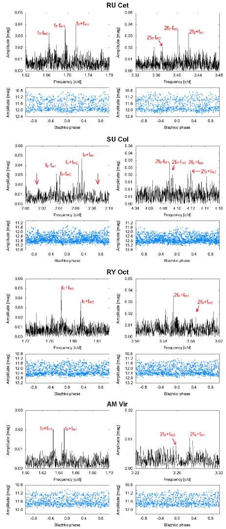
Figure 6: Four stars from our ASAS sample with double/irregular modulation. The first column depicts Fourier transform in the vicinity of $f_{0}$ after prewhitening with the main pulsation components and data phased with period corresponding to $f_{m1}$. There is the vicinity of $2f_{0}$ and phase plot according to the second modulation period (related to $f_{m2}$) in the second column.

4.2 Stars suspected of multiple/irregular modulation and IK Hya

In the bottom part of Table 1 there are six stars we suspect of some peculiarity in their modulations. All these stars showed additional peaks around $f_{0}$ probably related to an additional modulation component. This behavior was described, for instance, in XZ Cyg (LaCluyzé et al. 2004), UZ UMa (Sodor et al. 2006), CZ Lac (Sódor et al. 2011), or more recently in V445 Lyr (Guggenberger et al. 2012). We also identified expected peaks around $2f_{0}$, which was a necessary condition to mark the stars as multiply modulated. Unfortunately, except for SU Col, these peaks had low amplitude under the confidence limit $S/N>4$. Prewhitened frequency spectra of these stars in the vicinity of $f_{0}$ and $2f_{0}$ with identification of the peaks are plotted in fig. 6. There are also phase-plots corresponding to suspected modulation periods in fig. 6.

SF07 identified SU Col as triple-modulated star. Peaks corresponding to periods 65 and 89 d (see fig. 6) were easily identified, while our analysis did not show any sign of the supposed 29.5-day period (the positions of peaks referring to this period are marked by an arrow in fig. 6). Residuals around additional peaks seem to be quite high, which can indicate that more peaks can be present but undetectable in the dataset. This, along with the absence of 29.5-day peak, could suggest that the Blazhko modulation of SU Col is irregular and changing.

A very interesting case of a possibly multiple/irregularly-modulated star is IK Hya (fig. 7). Its frequency spectra are somewhat confusing. There are two strong triplets ($f_{m1l},f_{0},f_{m1r}$ and $f_{m2l},f_{0},f_{m2r}$, where indexes $l$ and $r$ mean ‘left’and ‘right’, $f_{m1r}=f_{0}+f_{m1}$, $f_{m1l}=f_{0}-f_{m1}$ and similarly for $f_{m2l}$ and $f_{m2r}$). Frequency $f_{m1}$ corresponds to a 71.81-day known period, $f_{m2}$ holds for the newly determined period of 1403 d. The spacing of the closer triplet was almost identical; i.e., $\Delta f=\left(f_{m2r}-f_{0}\right)-\left(f_{0}-f_{m2l}\right)=4\cdot 10^{-5}$, while the offsets of wider peaks from $f_{0}$ were identical only roughly ($\Delta f=6.9\cdot 10^{-4}$). This discrepancy resulted in an inequality of the first modulation period based on the left peak (75.57 d) and the right peak (71.81 d). Thus, these peaks might indicate two independent periods or limiting values of changing modulation period.

This is supported by the identification of symmetric counterparts of $f_{m1l}$ and $f_{m1r}$ with respect to $f_{0}$, which we found in frequency spectra, but which had amplitudes close to $S/N=4$. The difference between the right-hand-side peaks $f_{m1r}$ and $f_{m2r}$ nearly equals $f_{0}-f_{m1l}$, in other words $75.57^{-1}\cong 71.81^{-1}+1403^{-1}$. This means that we actually observed one narrow triplet $f_{m2l},f_{0},f_{m2r}$ and two doublets (one on each side of $f_{0}$) with spacing corresponding to 1403-d period. This could indicate a 1403-day long-term cycle, during which the Blazhko and pulsation characteristics are changing similarly to the four-year cycle of RR Lyr (Detre & Szeidl 1973; Stellingwerf et al. 2013). A very interesting and possibly important thing is that the long period (1403 d) is very close to half of the beating period of 75.57 d and 71.81 d periods, which is 2886 days.

Table 2: New Blazhko stars from our ASAS sample

Star	Epoch HJD	$P_{\mathrm{puls}}$ [d]	$P_{\mathrm{BL}}$ [d]	$A_{-}$ [mag]	$A_{+}$ [mag]	$A_{+}/A_{-}$	$n$	$TS$ [d]
EL Aps	2451870.4229	0.5797216(5)	25.96(2)	-	0.019	-	849	3275
HH Aqr	2451889.5259	0.574434(1)	3360(270)	-	0.057	-	395	3274
LS Boo	2453103.7768	0.552704(2)	42.28(9)	-	-	-	359	2371
UY Boo	2454289.5426	0.650902(2)	171.8(2)	-	0.038	-	312	2907
V595 Cen	2453835.6569	0.691035(1)	107.5(6)	-	0.025	-	656	3188
RW Hyi	2454150.5160	0.555791(1)	135.2(6)	0.048	0.036	0.75	654	3296
AO Lep	2453767.6882	0.5600866(7)	93.0(1)	0.048	0.044	0.92	570	3296
XZ Mic	2452757.8704	0.4491584(4)	85.7(3)	-	-	-	595	3238
V784 Oph	2452775.7903	0.603359(1)	25.61(2)	-	0.044	-	352	2884
ASAS173154-1653.1	2453864.7477	0.602590(1)	52.41(8)	-	0.014	-	453	3145
CY Peg	2453337.5595	0.647939(2)	464(5)	0.071	-	-	238	2349
RU Scl	2452141.8678	0.4933549(2)	23.91(2)	-	0.010	-	338	3262
AE Scl	2452213.5875	0.5501123(9)	46.2(2)	-	0.046	-	497	3243
V Sex	2454633.4803	0.487372(1)	118.5(4)	-	0.061	-	317	2570
SS Tau	2453046.5674	0.3699068(7)	123.3(4)	-	0.057	-	320	3220
HH Tel	2451963.8028	0.4820925(5)	143(2)	-	-	-	518	3166
FS Vel	2454618.5425	0.4757576(5)	59.29(7)	-	0.040	-	618	3300
UV Vir	2451887.0160	0.5870842(7)	103.9(3)	-	0.027	-	365	3163
AF Vir	2454678.5669	0.483747(1)	42.15(5)	-	0.041	-	340	2915

In SW data only one slightly asymmetric triplet (Blazhko effect with period 73.2 d) was identified. This period would support the theory of changing Blazhko effect of IK Hya rather than compound modulation with three periods. With ASAS and SW data, it is impossible to perform a more detailed analysis. Therefore, IK Hya is an object that deserves to be investigated much more closely with larger telescopes than for automated surveys.

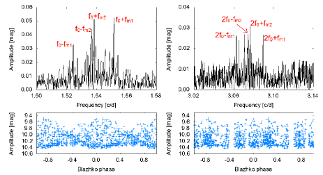
Figure 7: IK Hya. Vicinity of $f_{0}$, $2f_{0}$ and light curves constructed with periods 71.81 d (bottom left) and 1403 d (bottom right). Frequency $f_{m1r}$ corresponds to 71.81 d, $f_{m1r}$ to 75.57 d , $f_{m2}$ to 1403 d.

4.3 New Blazhko stars

There are 19 new Blazhko stars in Table 2, which were not identified by WS05 or by SF07. Only two of the newly revealed Blazhko variables showed a triplet structure, which is probably a consequence of weak Blazhko effect manifestation. V784 Oph is actually not a new Blazhko star, because we discovered the modulation at the same time as de Ponthiere et al. (2013), who identified its multiple modulation (our analysis showed only simple modulation).

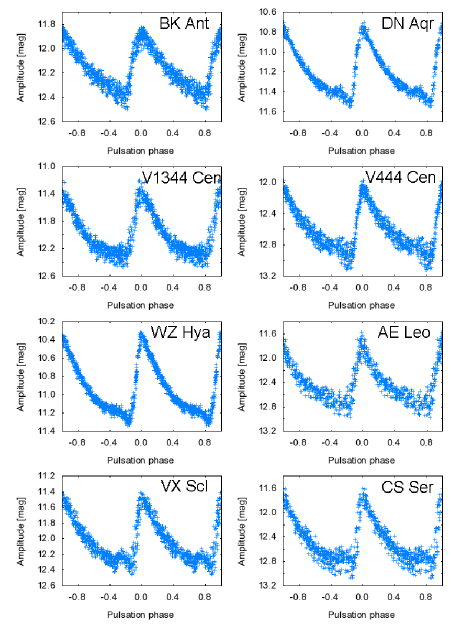
Figure 8: Possible Blazhko stars. Data are phased with respect to ephemerides given in Table 3.

In the case of LS Boo, XZ Mic, and HH Tel, their modulation periods are based on the side peaks with $S/N$ slightly lower than 4, but their Blazhko phased light curves look good (fig. 9). Comparing the Blazhko periods of HH Tel and of XZ Mic with values coming from the SW data (Table 5) we see that they are real and nearly have the same value. This raises the question, if the significance condition $S/N>4$ should not be lowered. HH Aqr have a somewhat uncertain Blazko period, because it is longer than the time span of the data.

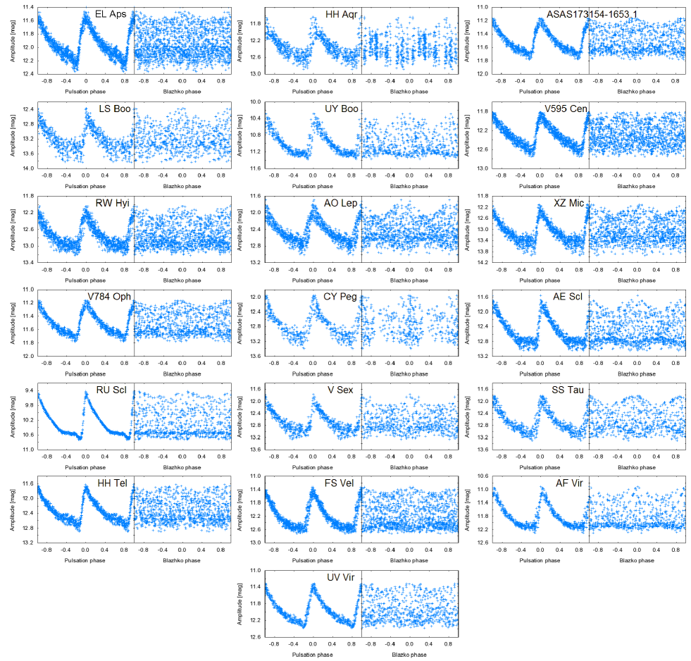
Figure 9: New Blazhko stars from ASAS database. Data are phased with respect to ephemerides given in tab. 2.

Frequency analysis of UY Boo showed, except for the modulation side peak, also another additional peak, which corresponds to the period 1976 d. This is probably the consequence of its peculiar period changes (Le Borgne et al. 2007).

Table 3: Stars suspected of the Blazhko effect

Star	Epoch HJD	$P_{\mathrm{puls}}$ [d]	$n$	$TS$ [d]
BK Ant	2454911.6407	0.5165704(6)	602	3169
DN Aqr	2452471.8336	0.6337573(4)	400	3219
V444 Cen	2452144.6919	0.5141328(6)	537	3194
V1344 Cen	2453890.5987	0.4182563(4)	594	3187
WZ Hya	2454838.7787	0.5377193(3)	628	3300
AE Leo	2452630.7110	0.626673(2)	421	2400
VX Scl	2451916.0250	0.637066(1)	552	3295
CS Ser	2453896.6210	0.5267982(8)	472	3168

The Blazhko effect of stars in Table 3 is somewhat ambiguous. These eight stars are candidate Blazhko variables. They show scattering around maxima (fig. 8), but not necessarily due to modulation – it can simply be the consequence of the scattering. There were peaks with $S/N<4$ identified in the Fourier spectrum of CS Ser, which could be caused by the Blazhko effect with period 118.3 d. Similar to the aforementioned cases of HH Tel and XZ Mic with the same characteristics, these peaks probably are real manifestations of the modulation.

Table 4: Known Blazhko stars from our SW sample.

Star	Epoch HJD	$P_{\mathrm{puls}}$ [d]	$P^{\mathrm{F}}_{\mathrm{BL}}$ [d]	$P^{\mathrm{M}}_{\mathrm{BL}}$	$A_{-}$ [mag]	$A_{+}$ [mag]	$A_{+}/A_{-}$	n	TS [d]	$P^{\mathrm{Lit}}_{\mathrm{BL}}$
DR And	2454334.5942	0.563112(6)	58.11(2)	58.2(3)	0.052	0.066	1.27	4536	705	57.5(1)
U Cae*	2453996.5377	0.41978515(5)	22.77(2)	22.7(5)	0.025	-	-	5252	491	22.8(2)
AH Cam	2454362.6540	0.368721(4)	10.772(6)	10.65(6)	0.034	0.075	2.21	1783	1227	10.83(2)
SS Cnc*	2454167.5509	0.367341(1)	5.419(9)	5.42(3)	0.012	-	-	3554	116	5.309(3)
Z Cvn	2456078.3420	0.653684(9)	22.48(2)	-	0.042	0.044	1.04	2086	121	22.98(2)
SS CVn	2453140.6137	0.4785195(2)	94.19(2)	94.26(9)	0.062	0.099	1.54	8811	1476	93.72(2)
RY Col*	2454423.3675	0.4788302(2)	82.35(2)	82.4(2)	0.027	0.074	2.74	9478	516	82.08(2)
DM Cyg	2454344.4237	0.4198639(8)	10.38(1)	10.7(1)	-	0.009	-	1940	473	10.57(4)
XZ Dra	2454686.4674	0.4765587(5)	-	75(1)	-	-	-	5807	83	73–77(5)
SS For*	2453997.4793	0.4954351(5)	34.73(1)	34.66(7)	0.03	0.059	1.97	8684	654	34.94(6)
RT Gru*	2454246.6550	0.5121845(6)	86.7(2)	87.8(3)	0.025	0.037	1.48	10238	537	87(7)
SV Hya*	2454528.4773	0.478546(2)	62.8(3)	63(2)	-	0.025	-	5374	131	63.29(8)
IK Hya*	2454155.5952	0.650247(4)	73.18(3)	73.2(3)	0.032	0.061	1.91	12856	754	67.5(2)
V559 Hya*	2454199.5359	0.4479571(2)	26.454(2)	26.47(2)	0.093	0.12	1.29	10055	754	26.6(7)
FU Lup	2454594.3086	0.3821526(3)	42.81(1)	42.74(9)	0.034	0.107	3.15	8300	752	42.49(8)
V1645 Sgr*	2454307.315	0.552955(3)	-	-	-	-	-	11310	754	1331.74(8)
BR Tau*	2454143.386	0.390600(1)	-	18.14	-	-	-	2063	139	19.3(9)
CD Vel*	2454151.3312	0.5735080(7)	66.34(4)	66.38(26)	0.016	0.023	1.44	14501	735	66.35(8)
Stars suspected of multiple modulation
RS Boo	2453132.5463	0.3773210(2)	41.3(2), 62.5(2)	64(3)	0.006, 0.006	0.010, 0.007	1.66, 1.16	3737	133	532.48(2)
RW Cnc	2454118.5843	0.547191(6)	29.14(8), 21.9(1)	30.0(3), 21.9(5)	0.021	0.012,0.014	0.57	3513	129	87(10)
RX Col*	2454106.4342	0.593743(1)	134.3(1), 79.7(2)	135.7(7), 81(2)	0.014	0.050, 0.011	3.57	11003	677	134.77(2)
RW Dra	2454655.5652	0.4429239(4)	41.42(1), 72.6(2)	41.49(5), 72.3(3)	0.055, 0.018	0.090, 0.013	1.64, 0.72	17386	492	41.42(2)

(1) Lee & Schmidt (2001); (2) Le Borgne et al. (2012); (3) Jurcsik et al. (2006); (4) Jurcsik et al. (2009b); (5) Jurcsik et al. (2002); (6) Kolenberg et al. (2009); (7) WS05; (8) SF07; (9) Jurcsik at al. (2009a); (10) Smith (1995).

5 Blazhko stars from SW

5.1 Known Blazhko stars

After a pre-selection of 243 RR Lyraes from SW data we obtained 106 stars for further analysis. Twenty-eight objects were proposed to show the Blazhko effect. For six of them (SW And, OV And, V Ind, U Tri, RY Com, and AR Per), no significant indication of the modulation was found. In RY Com and AR Per, this was due to limited precision of used data, because they are modulated stars (Jurcsik at al. 2009a; Watson et al. 2006).

Twenty-two remaining known Blazhko stars are listed in Table 4. The fifth column gives the modulation period based on frequency analysis ($P^{\mathrm{F}}_{\mathrm{BL}}$), and the sixth ($P^{\mathrm{M}}_{\mathrm{BL}}$) gives the Blazhko period based on the $Mag_{\mathrm{max}}$ vs. $T_{\mathrm{max}}$ analysis. The last column provides modulation periods known from literature. Other columns correspond with those in Table 1. An asterisk in the first column (if present) indicates that the data were also available in the ASAS survey. The times ($T_{\mathrm{max}}$) and magnitudes $Mag_{\mathrm{max}}$ of maxima (Table 5) can be found in electronic form as an on-line material at the CDS portal.

Table 5: Times and magnitudes of maximum light of 35 stars from SW survey, which is available in electronic form.

Star	HJD $T_{\mathrm{Max}}$	errHJD	Max [mag]	errMax
DR And	2454325.5842	4	11.972	4
	2454330.6559	9	11.832	12
…	…	…	…	…

Frequency spectra of almost all SW stars were affected by artificial effects, such as small shifts in the data from different nights or by gaps between observations, which resulted in additional peaks near $f_{0}$ with no clear interpretation. Peaks corresponding to the time span of the data occurred frequently.

In XZ Dra and BR Tau, the Blazhko effect was not detected in their frequency spectra, but it was noted in the change of maximum magnitude. V1645 surely showed modulation, but SW data were in this case insufficient for determining the Blazhko period.

5.2 SW Stars suspected of multiple/irregular modulation

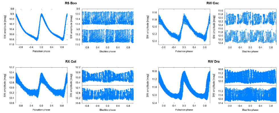
Figure 10: Known Blazhko stars with more than one modulation period. In the left panel of each star the data are folded with respect to the basic pulsation period. On the left, panels are data-phased with modulation periods.

Four known Blazhko variables in our SW sample were identified as stars with multiple modulation (the bottom part of Table 4, fig. 10). RS Boo, RW Cnc and RW Dra were suspected of such behaviour in the past; RX Col is a newly discovered as multiple modulated star (it was known as single-modulated star).

The Blazhko period of $\sim$533 d of RS Boo has been known for a long time (Oosterhoff 1946), but there have been some indications of additional periodicity. Kanyo (1980) reported another period in the range of 58-62 days, but Nagy (1998) did not observe it. There was no indication of a 533 d period in SW data – probably due to the time span of only 133 d. During the analysis we revealed a period of 62.5 d, which is close to the period noted by Kanyo (1980). Except for this period we also noted obvious indications of a period of 41.3 d.

Balazs & Detre (1950) reported RW Cnc to be a double-modulated star with modulation periods 29.95 and 91.1 d. The first modulation period was determined as 29.14 d (30.0 d from maxima analysis), and the second period 21.9 d from both frequency and maxima analysis. No indications of a 91-day cycle were found. The 87-day period given by Smith (1995) was also not observed.

RW Dra was found to be multiple-modulated by Balazs & Detre (1952). A Blazhko period of 41.61 d was accompanied by periods of 124 d and two other periods with lengths of years. We noted the Blazhko period of 41.42 d and only one secondary modulation period with a length of 72.6 d.

These four stars have a very interesting feature – the modulation periods are very close to a resonance with small integers: $\left(P_{m2}/P_{m1}\right)_{\mathrm{RS\leavevmode\nobreak\ Boo}}=1.513\cong$ 3:2; $\left(P_{m1}/P_{m2}\right)_{\mathrm{RW\leavevmode\nobreak\ Cnc}}=1.331\cong$ 4:3; $\left(P_{m1}/P_{m2}\right)_{\mathrm{RX\leavevmode\nobreak\ Col}}=1.685\cong$ 5:3 and $\left(P_{m2}/P_{m1}\right)_{\mathrm{RW\leavevmode\nobreak\ Dra}}=1.753\cong$ 7:4. In the ASAS stars only the modulation periods of SU Col approximate the resonance 4:3 ($P_{m2}/P_{m1}=1.369$). This seems very odd. Either the resonances are some strange consequence of SW data or the stars behave similarly to CZ Lac, where resonances of the modulation periods were also observed (Sódor et al. 2011).

Table 6: New Blazhko stars from our SW sample.

Star	Epoch HJD	$P_{\mathrm{puls}}$ [d]	$P^{\mathrm{F}}_{\mathrm{BL}}$ [d]	$P^{\mathrm{M}}_{\mathrm{BL}}$	$A_{-}$ [mag]	$A_{+}$ [mag]	$A_{+}/A_{-}$	n	TS [d]
XX Boo	2454267.5088	0.5813995(3)	105.9(1)	105.6(3)	0.012	0.015	1.25	8707	1150
V595 Cen*	2454239.2256	0.6910344(5)	107.41(9)	107.6(2)	0.004	0.019	4.75	15709	754
GY Her	2454619.5950	0.524244(6)	49.6(2)	49.1(9)	0.049	0.053	1.08	8065	108
XZ Mic*	2453964.2968	0.4491569(6)	85.8(2)	85.7(5)	0.034	0.035	1.03	8591	537
TU Per	2454438.5346	0.6070469(4)	59.0(3)	-	0.021	0.015	0.71	2383	108
RU Scl*	2454364.4311	0.493368(1)	23.6(1)	24.0(3)	0.003	0.008	2.67	3725	103
V4424 Sgr	2453881.6352	0.4245024(2)	29.28(4)	27.62(8)	0.005	0.004	0.80	8778	528
HH Tel*	2454347.2643	0.482056(5)	-	133(9)	-	-	-	2761	93
FS Vel*	2454201.2979	0.4757597(2)	59.48(4)	59.1(2)	0.020	0.026	1.30	9677	713
Stars suspected of multiple/irregular modulation
RZ CVn	2454263.4059	0.567418(-)	33.35-33.26	29.6-33.36	0.007	0.017	2.43	7148	1136
AG Her	2454669.4418	0.6494465(3)	79.69(7), 47.93(7)	79.58(7),47.96(2)	0.010, 0.014	0.030, 0.020	3, 1.43	22362	1552
AE Scl*	2453920.5919	0.550116(2)	46.07(2), 104.7(2)	46.04(4)	0.019, 0.019	0.044, 0.015	2.32, 0.79	8179	563

5.3 New Blazhko stars from SW

Nine new, previously unknown single-modulated Blazhko stars, were identified in our SW sample (Table 6, fig. 12). For six of these stars (marked by an asterisk) ASAS data were also available. Three stars showed double modulation or some peculiarity in their Blazhko effect.

RZ Cvn (fig. 11) seemed to change its Blazhko period. In the first part of the used data (between HJD 2453130 and 2453249), the Blazhko period was 33.35 d (29.6 d on the basis of maxima analysis), the amplitude of the modulation was 0.104 mag (peak to peak) and $A_{1}=0.339$ mag, while between HJD 2454135 and 2454266, the Blazhko cycle lasted 33.26 d (33.4 d based on maxima analysis). The amplitude of the modulation was almost twice as big as in the first part (0.192 mag) and $A_{1}=0.363$ mag. The basic pulsation period also changed slightly (0.567411 vs. 0.567418 d). Similar behaviour is known in, say, XZ Dra (Jurcsik et al. 2002) or RV UMa (Hurta et al. 2008). We point out that in the case of RZ CVn, the Blazhko periods determined on the basis of maxima analysis offer better confidence.

The second multiple-modulated star, AG Her, shows possible resonances of its modulation periods $\left(P_{m1}/P_{m2}\right)_{\mathrm{AG\leavevmode\nobreak\ Her}}=1.659\cong$ 5:3 similar to RX Col, and another three stars discussed in previous section. AE Scl was identified as single-modulated in the ASAS data set.

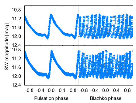
Figure 11: RZ CVn in different seasons. Change in the light variations, as well as in the amplitude of the modulation is noticeable.

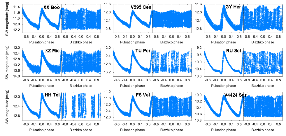
Figure 12: New Blazhko stars from SW database. Light curves are constructed according to ephemerides listed in Table 6.

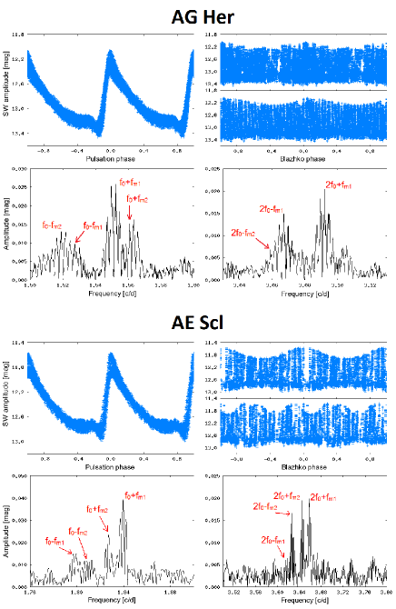
Figure 13: Data of AG Her and AE Scl folded with elements given in Table 6 and with their frequency spectra in the vicinity of $f_{0}$ and $2f_{0}$. In Blazhko phased data of AE Scl it is apparent that the second modulation period should instead be 104.7/2 than 104.7 d, but the frequency spectra indicated period 104.7 d.

6 Statistics of the Blazhko variables in the sample

From the sample containing 321 RRab type stars, one hundred objects were identified as Blazhko variables. This means that the incidence rate of Blazhko stars among RRab sample stars was 31 %. If we include certain Blazhko variables, whose modulation was not detectable (5), this percentage would grow almost to 33 %. If Blazhko candidates (8) are also taken into account, this rate would be 35 %. Finally, if all suspected stars are included (18 instead of 5), the percentage would be 39 %. In addition, it is likely for this number to be slightly higher, in fact, because the modulation of a number of stars with low modulation amplitude might remained uncovered.

Compared to incidences 5.1 % (SF07) and 4.3 % (Wils et al. 2006), our percentage is significantly higher and roughly approximates the percentage based on precise measurements – 48 % (Benkő et al. 2010) based on Kepler data, or 47 % (Jurcsik at al. 2009a), who utilized precise ground-base observations.

Our incidence is also higher than in LMC (20 %, Soszyński et al. 2009) or than in SMC (22 %, Soszyński et al. 2010). In the Galactic bulge this rate is about 25 % (Mizerski 2003). It is worth mentioning that these numbers almost doubled during the past few years owing to more sensitive analysis techniques and an increase in the time span of the data. It is likely that these numbers will also increase slightly in future works.

About 60 % of confirmed Blazhko variables were of BL2 type. Considering ASAS and SW surveys separately, this rate was 48 % (ASAS) and 76 % (SW). Several stars in the SW sample turned out to be of BL2, while in ASAS they were BL1 type. This finding clearly shows that classification of the stars based on their side-peak distribution strongly depends on data quality and should not be used when analysing low-quality data, which is known (Alcock et al. 2003). In addition, ultra-precise space measurements showed that almost every modulated star has peaks on both sides. Our recommendation is also supported by the fact that the percentage of stars, which show $A_{+}/A_{-}>1$, was about 89 % in our ASAS sample contrary to 51% given by SF07.

The distribution of newly discovered Blazhko variables in $P_{\mathrm{BL}}$ vs. $P_{\mathrm{puls}}$ diagram displayed in fig. 14 is random, and no dependency between the pulsation and Blazhko periods was found, as expected.

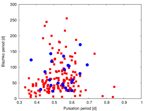
Figure 14: $P_{\mathrm{BL}}$ vs. $P_{\mathrm{puls}}$ diagram of known RRab Blazhko stars. Red squares represent known Blazhko stars taken from the on-line database BlaSGalF (Skarka 2013). Recently discovered Blazhko stars are plotted as blue circles. Stars with periods over 300 d are not showed for a clearer arrangement.

Twelve stars in our sample turned out to be multiple-modulated and/or with changing Blazhko effect, which is 12 % of all studied Blazhko stars. Until today only a few stars have been known to show such behaviour. Again, it is very likely that compound modulation is more common than astronomers thought and that the number of known multiple-modulated stars will increase in future analyses.

7 Conclusions

A period study of 321 fundamental mode galactic field RR Lyraes with brightness at maximum light higher than 12.5 mag was performed based on available data from the ASAS and/or SW database. These stars were chosen from a more extended sample consisting of 557 stars after careful pre-selection based on conditions described in sec. 2. Each light curve was cleaned and analysed individually. In addition, each frequency spectrum was scanned through careful visual inspection to avoid omitting any sign of the Blahzko effect.

One hundred stars were identified and confirmed to be Blazhko variables (25 previously unknown). Eight stars, marked as Blazhko candidates, showed some ambiguous indications of modulation like characteristic scattering around maximum of phased light curve. In contrast no indication of the Blazhko behaviour was found in 18 stars, which were supposed to be modulated. However, five of these eighteen stars are certain Blazhko variables, but with too small amplitude of modulation to be detectable in ASAS or SW data.

The incidence rate of RRab Blazhko stars from our analysis is at least 31 %, which is a much higher percentage than given by previous studies based on data from surveys with similar data quality. This increase would be logically expected, since more time-extended datasets were examined (in many cases simultaneously in ASAS and SW surveys). However, it is still less than the incidence rates determined in the framework of precise ground-base and space surveys. With certainty there remained undetected low-amplitude Blazhko variables, as well as stars with the shortest and the longest modulation periods, simply due to nature of the data from ASAS and SW surveys.

A surprising result was a very high incidence of stars with some peculiarity in their Blazhko effect – each eighth star of our Blazhko sample showed signs of the changes in Blazhko effect or compound modulation. An interesting examples are IK Hya and RZ CVn. Both stars probably undergo changes in their pulsation and modulation characteristics. IK Hya could be another star with a few-year-long cycle analogical to four-year cycle in RR Lyrae itself. Five of ten identified multiple-modulated stars showed the ratio between their modulation periods in ratio of small integers.

Our study confirmed that classification and statistics of modulated stars according to their side peaks, which are based on low-quality data, are not reliable. It was also shown that the sensitivity of automatic procedures used to identify the Blazhko effect is insufficient – one fourth of the Blazhko variables were identified for the first time. It is likely that the incidences and characteristics of Blazhko variables identified in other surveys (e.g. in LMC based on OGLE, Alcock et al. 2003) could be slightly different than proposed. Our conclusions should serve as a challenge for developing better tools for automatic data analysis, because a manual examination of many thousand stars is impossible to perform.