Bayesian nonparametric dependent model for partially replicated data: the influence of fuel spills on species diversity

Abstract

We introduce a dependent Bayesian nonparametric model for the probabilistic modeling of membership of subgroups in a community based on partially replicated data. The focus here is on species-by-site data, i.e. community data where observations at different sites are classified in distinct species. Our aim is to study the impact of additional covariates, for instance environmental variables, on the data structure, and in particular on the community diversity. To that purpose, we introduce dependence a priori across the covariates, and show that it improves posterior inference. We use a dependent version of the Griffiths–Engen–McCloskey distribution defined via the stick-breaking construction. This distribution is obtained by transforming a Gaussian process whose covariance function controls the desired dependence. The resulting posterior distribution is sampled by Markov chain Monte Carlo. We illustrate the application of our model to a soil microbial dataset acquired across a hydrocarbon contamination gradient at the site of a fuel spill in Antarctica. This method allows for inference on a number of quantities of interest in ecotoxicology, such as diversity or effective concentrations, and is broadly applicable to the general problem of communities response to environmental variables.

1 Introduction

This paper was motivated by the ecotoxicological problem of studying communities, or groups of species, observed as counts of species at a set of sites, where the composition and distribution of species may differ among sites, and for which the sites are indexed by a contaminant. More specifically, the soil microbial data set we are focusing on in this paper was acquired at different sites of a fuel spill region in Antarctica. Although there is now much greater awareness of human impacts on the Antarctic, substantial challenges remain. One of these is the containment of historic buried station waste, chemical dumps and fuel spills. These wastes do not break down in such extreme environments and their spread is exacerbated by melting ice in summer. In order to develop effective containment strategies, it is important to understand the impact of these incursions on the natural environment. The data set considered here consists of soil microbial counts of operational taxonomic units, OTUs, as well as a site contaminant level measured by the total petroleum hydrocarbon, TPH. Thus the aim is to model the probabilities of occurrence associated with the species at the different sites and to be able to interpret the impact of the contaminant on the community as a whole or on a particular species.

This specific case study gives rise to a more general problem that can be described as modeling the probability of membership of subgroups of a community based on partially replicated data obtained by observing different subsets of the subgroups at different levels of a covariate. The problem can also be considered as the analysis of compositional data in which the data points represent so called compositions, or proportions, that sum to one. A typical example is the chemical composition of rock specimens in the form of percentages of a pre-specified number of elements (see e.g. Aitchison,, 1982; Barrientos et al.,, 2015). More generally, the problem is endemic in many fields such as biology, physics, chemistry and medicine. Despite this, the solution to that problem remains a challenge. Common approaches are typically based on parametric assumptions and require pre-specification of the number of subgroups (e.g., species) in the community. In this paper, we suggest an alternative that overcomes this drawback. The method is described in terms of species for reasons of intuitiveness in description, nevertheless, the approach is generally applicable far beyond the species sampling framework.

We propose a Bayesian nonparametric approach to both the specific and general problems described above, using a covariate dependent random probability measure as a prior distribution. Dependent extensions of random probability measures, with respect to a covariate such as time or position, have been extensively studied recently under three broad constructions. First, a class of solutions is based on the Chinese Restaurant process; see for instance Caron et al., (2007); Johnson et al., (2013). These are oriented towards in-line data collection and fast implementation. Second, some approaches use completely random measures; see for example, Lijoi et al., 2013a ; Lijoi et al., 2013b . An appealing feature of this approach is analytical tractability, which allows for more elaborate studying of the distributional properties of the measures. Third, many strategies make use of the stick-breaking representation, based on the line of research pioneerd by MacEachern, (1999, 2000) which define dependent Dirichlet processes. See its plentiful variants which include Griffin and Steel, (2006, 2011); Dunson et al., (2007); Dunson and Park, (2008); Chung and Dunson, (2009) among others. The success of the stick-breaking constructions stems from their attractiveness from a computational point of view as well as their great flexibility in terms of full support, which we prove for our model in Section S.3.2 of Supplementary Material. This is the approach that we follow here.

We define a dependent version of the Griffiths–Engen–McCloskey distribution (hereafter denoted $\mathsf{GEM}$), which is the distribution of the weights in a Dirichlet process, for modeling presence probabilities. Dependence is introduced via the covariance function of a Gaussian process, which allows dependent Beta random variables to be defined by inverse cumulative distribution functions transforms. The resulting model is not confined to the estimation of diversity indices, but could also utilize the predictive structure yielded by specific discrete nonparametric priors to address issues such as the estimation of the number of new species (subgroups) to be recorded from further sampling, the probability of observing a new species at the $(n+m+1)$-th draw conditional on the first $n$ observations, or of observing rare species, where by rare species one refers to species whose frequency is below a certain threshold (see e.g. Lijoi et al.,, 2007; Favaro et al.,, 2012).

The paper is organized as follows. In Section 2 we describe our case study, review the ecotoxicological literature and background, and discuss diversity and effective concentration estimation. Section 3 describes the Bayesian nonparametric model, posterior sampling and most useful properties of the model. Estimation results and ecotoxicological guidelines are given in Section 4. A discussion on model considerations is given in Section 5 and Section 6 concludes this paper with a general discussion. Extended results, details of posterior computation and the proofs of our results are available in Supplementary Material available as Arbel et al., 2015c .

2 Case study and ecotoxicological context

2.1 Case study and data

As already sketched in the Introduction, our case study consists in a soil microbial data set acquired across a hydrocarbon contamination gradient at the location of a fuel spill at Australia’s Casey Station in East Antarctica ($110^{\circ}\,32^{\prime}$ E, $66^{\circ}\,17^{\prime}$ S), along a transect at 22 locations. Microbes are classified as Operational Taxonomic Units (OTU), that we also generically refer to as species throughout the paper. OTU sequencing were processed on genomic DNA using the mothur software package, see Schloss et al., (2009). We refer to Snape et al., (2015) for a complete account on the data set acquisition. The total number of species recorded at least once at one site is 1,800+. All species were included in the estimation. However, we have noticed that it is possible to work with a subset of the data, consisting of those species with abundance over all measurements exceeding a given low threshold (say up to ten), without altering significantly the results. A crucial point for the subsequent analyses is that we order the species by decreasing overall abundance, i.e. species $j=1$ is the most numerous species in the whole data set. The variations of sampling across the sites explain why the species are not strictly ordered when considered site by site, see Figure 1.

OTU measurements are paired with a contaminant called Total Petroleum Hydrocarbon (TPH, see Siciliano et al.,, 2014), suspected to impact OTU diversity. The contamination TPH level recorded at each site ranges from 0 to 22,000 mg TPH/kg soil. Ten sites were actually recorded as uncontaminated, i.e. with TPH equal to zero. We call the microbial communities associated to these sites baseline communities, and use them in order to define effective concentrations $EC_{x}$, see Section 2.4. Although a continuous variable, TPH is recorded with ties that we interpret as due to measurement rounding. We jitter TPH concentrations with a random Gaussian noise (absolute value for the case TPH = 0) in order to account for measurement errors and to discriminate the ties. This noise can be incorporated in the probabilistic model. Reproducing estimation for varying values of the variance of the noise, moderate compared with the variability of TPH, have shown little to no alteration of the results.

2.2 Ecotoxicological context

This paper focuses on an ecotoxicological case study where the goal is to predict the impact of a contaminant on an ecosystem. The common treatment of this question relies on toxicity tests, either on single species (called populations) or on multiple species (called communities). The need for appropriate modeling techniques is apparent due to data limitations, for instance in our case where data acquisition in Antarctica is extremely expensive. If single species modeling methods are now well comprehended, community modeling still lacks from theoretical evidence endorsement. There are two alternative community modeling approaches. On one hand, one can model single species independently and then aggregate the individual predictions into community predictions (e.g. Ellis et al.,, 2011). A drawback attached to the aggregation is the lack of appropriate uncertainty of the method, on top of which one necessarily lose crucial information by dismissing interplays across species. On the other hand, the response of the community as a whole is modeled, which generally entails the use of some univariate summaries of community responses, such as compositional dissimilarity (e.g. Ferrier and Guisan,, 2006; Ferrier et al.,, 2007) or rank abundance distributions (Foster and Dunstan,, 2010). Alternatively, the responses of multiple species can be modeled simultaneously (e.g. Foster and Dunstan,, 2010; Dunstan et al.,, 2011; Wang et al.,, 2012).

Single species are commonly modeled through the probability of presence $p_{j}$ of each species $j$ as a function of the environmental parameters. The natural distribution for multiple species is the multinomial distribution, which provides an intuitive framework when the sampling process consists of independent observations of a fixed number of species. Recent literature demonstrates the popularity of the multinomial distribution in ecology (e.g. Fordyce et al.,, 2011; De’ath,, 2012; Holmes et al.,, 2012) and genomics (Bohlin et al.,, 2009; Dunson and Xing,, 2009). Our use of the $\mathsf{GEM}$ distribution actually extends the multinomial distribution to cases where the number of species does not need be neither fixed nor known, i.e. where the prior is on infinite vectors of presence probabilities.

2.3 Diversity

Modeling presence probabilities provides a clear link to indices that describe various community properties of interest to ecologists, such as species diversity, richness, evenness, etc. The literature on diversity is extensive, not only in ecology (Hill,, 1973; Patil and Taillie,, 1982; Foster and Dunstan,, 2010; Colwell et al.,, 2012; De’ath,, 2012) but also in other areas of science, such as biology, engineering, physics, chemistry, economics, health and medicine (see Borges and Roditi,, 1998; Havrda and Charvát,, 1967; Kaniadakis et al.,, 2005), and in more mathematical fields such as probability theory (Donnelly and Grimmett,, 1993). There are numerous ways to study the diversity of a population divided into groups, examples of predominant indices in ecology include the Shannon index $-\sum_{j}p_{j}\log p_{j}$, the Simpson index (or Gini index) $1-\sum_{j}p_{j}^{2}$, on which we focus in this paper, and the Good index which generalizes both $-\sum_{j}p_{j}^{\alpha}\log^{\beta}p_{j}$, $\alpha,\beta\geq 0$ (Good,, 1953).

Diversity estimation, and more generally estimation of community indices based on species data, has been a statistical problem of interest for a long time. One of the reasons for that problem is simple and can be traced back to the high variability inherent to species data. For instance the most obvious estimators, hereafter referred to as empirical estimators, which consist in plugging in empirical presence probabilities, i.e. observed proportions $\hat{p}_{ij}$ of species $j$ at site $i$, suffer from that curse. Many treatments were proposed in the literature to account for this issue. An first approach is the field of occupancy modeling and imperfect detection, see for instance the monograph Royle and Dorazio, (2008). We provide a concise description of imperfect detection modeling in Section 5.1 and do not pursue this direction here. Another approach, that we follow in this paper, consists in smoothing, or regularizing, empirical estimates. A Bayesian approach is a natural way to do so. Specifically, Gill and Joanes, (1979) show that using a Dirichlet prior distribution over $(p_{1},\ldots,p_{J})$ in the multinomial model with $J$ species greatly improves estimation over empirical counterparts. The reason for this is that using a prior prevents pathological behaviors due to outliers by smoothing the estimates. The smoothing is controlled by the Dirichlet parameter which can be conducted according to expert information. Compared to the framework of Gill and Joanes, (1979), there is additional variability across sites in our case study. To instantiate this high variability of the empirical estimates of Simpson diversity, see their representation (dots) on Figure 4. However, we leverage this additional difficulty by borrowing of strength across the sites by following the intuition that neighboring sites should respond similarly to contaminant. The borrowing of strength is done by incorporating dependence across the sites in the prior distribution. In order not to impose the total number of species to be known a priori, we adopt a Bayesian nonparametric approach, hence extending the work by Gill and Joanes, (1979) from Dirichlet prior distributions to covariate-dependent Dirichlet process prior. This is also extending the model of Holmes et al., (2012) to a covariate-dependent setting with a priori unknown number of species. Note that this idea of using a Bayesian nonparametric approach as a smoothing technique for species data was recently adopted in the context of discovery probability, the probability of observing new species or species already observed with a given frequency. Good, (1953) proposed smoothed estimators popularized as Good–Turing estimators for discovery probabilities. Good–Turing estimators were shown to have a Bayesian nonparametric interpretation (see Lijoi et al.,, 2007; Favaro et al.,, 2015; Arbel et al., 2015a, ), which demonstrate the ability of Bayesian nonparametric methods to regularize species data.

2.4 Effective concentration

Highly relevant in terms of protecting an ecosystem, the effective concentration at level $x$, denoted by $EC_{x}$, is the concentration of contaminant that causes $x$% effect on the population relative to the baseline community (e.g. Newman,, 2012). For example, the $EC_{50}$ is the median effective concentration and represents the concentration of a contaminant which induces a response halfway between the control baseline and the maximum after a specified exposure time. For single species studies, this is commonly assessed by an $x$% increase in mortality. In applications with a multi species response as we are interested in this paper, it is the response of the community as a whole that is of interest. The $EC_{x}$ values are used to derive appropriate protective guidelines on contaminant concentrations, for instance in terms of waste, chemical dumps and fuel spills containment strategies. Currently, it is not clear how to best calculate $EC_{x}$ values using whole-community data. The $EC_{x}$ values can be defined in many ways depending on the specific aspects of interest to the ecological application. We illustrate the use of the Jaccard dissimilarity index, denoted by $\text{Jac}(X)$, one of the many dissimilarity variants available, as a measure of change in community composition. We defined the baseline community as the set of uncontaminated sites (ten sites), where TPH equals zero, see Section 2.1. The dissimilarity at TPH zero, denoted by $\text{Jac}_{0}$, is an estimate of the variability in community composition between uncontaminated sites. The $EC_{x}$ value is the smallest TPH value $X$ such that

$$\text{Jac}(X)=1-(1-\text{Jac}_{0})(1-x/100).$$ (1)

In this way, $EC_{0}$, the TPH value for which there is no change relative to baseline, is obtained at $\text{Jac}(X)=\text{Jac}_{0}$, while $EC_{100}$ is obtained at $\text{Jac}(X)=1$, i.e. for a TPH value such that the community composition becomes disjoint with the baseline. We see by Equation (1) that intermediate values are obtained by linear interpolation. The smallest TPH value is used so as to provide a conservative $EC_{x}$ estimate, since the dissimilarity curve is not guaranteed to be monotonic. A particular feature of the model which allows us to follow this methodology is its ability to estimate the community composition between observed TPH values, since it is unlikely that the dissimilarity threshold $\text{Jac}(X)$ sought in Equation (1) will coincide exactly with one of the measured TPH levels in the data. $95\%$ credible bands for $EC_{x}$ values were obtained in a similar fashion, i.e. as the smallest and the largest values of, respectively, the $2.5\%$ and $97.5\%$ quantiles of the $EC_{x}$ value, again so as to provide conservative estimates. See Figure 5 for an illustration of the method.

3 Model

3.1 Data model

We describe here the notations and the sampling process of covariate-dependent species-by-site count data. To each site $i=1,\ldots,I$ corresponds a covariate value $X_{i}\in\mathcal{X}$, where the space $\mathcal{X}$ is a subset of $\mathbb{R}^{d}$. We focus here on a single covariate, i.e. $d=1$. The general case $d\geq 1$ is discussed in Section 6. Individual observations $Y_{n,i}$ at site $i$ are indexed by $n=1,\ldots,N_{i}$, where $N_{i}$ denotes the total abundance, or number of observations. Observations $Y_{n,i}$ take on positive natural numbers values $j\in\{1,\ldots,J_{i}\}$ where $J_{i}$ denotes the number of distinct species observed at site $i$. No hypothesis is made on the unknown total number of species $J=\max_{i}J_{i}$ in the community of interest, which might be infinite. We denote by $(\mathbf{X},\mathbf{Y})$ the observations over all sites, where $\mathbf{X}=(X_{i})_{i=1,\ldots,I}$, $\mathbf{Y}=(\mathbf{Y}_{i}^{N_{i}})_{i=1,\ldots,I}$ and $\mathbf{Y}_{i}^{N_{i}}=(Y_{n,i})_{n=1,\ldots,N_{i}}$. The abundance of species $j$ at site $i$ is denoted by $N_{ij}$, i.e. the number of times that $Y_{n,i}=j$ with respect to index $n$. The relative abundance satisfies $\sum_{j=1}^{J_{i}}N_{ij}=N_{i}$.

We model the probabilities of presence $\mathbf{p}=(\mathbf{p}(X_{i}))_{i=1,\ldots,I}=(p_{j}(X_{i})_{j=1,2,\ldots})_{i=1,\ldots,I}$, where $p_{j}(X_{i})$ represents the probability of species $j$ under covariate $X_{i}$, by the following

$$Y_{n,i}\,|\,\mathbf{p}(X_{i}),X_{i}\,\operatorname*{\sim}\limits^{\scriptscriptstyle\text{ind}}\,\sum_{j=1}^{\infty}p_{j}(X_{i})\delta_{j},$$ (2)

for $i=1,\ldots,I$, $n=1,\ldots,N_{i}$, where $\delta_{j}$ denotes a Dirac point mass at $j$.

3.2 Dependent prior distribution

We follow a Bayesian approach, which implies that we need to define a prior distribution for the probabilities $\mathbf{p}$. The Dirichlet process (Ferguson,, 1973) is a popular distribution in Bayesian nonparametrics which has been used for modeling species data by Lijoi et al., (2007). We extend the methodology developed by Lijoi et al. in building a covariate-dependent prior distribution in a way which is reminiscent of the extension of the classical Dirichlet process to the dependent Dirichlet process by MacEachern, (1999). More specifically, the marginal prior distribution on $\mathbf{p}(X)$ for covariate $X$ is defined by the following stick-breaking construction, which introduces Beta random variables $V_{j}(X)\,\operatorname*{\sim}\limits^{\scriptscriptstyle\text{iid}}\,\mathsf{Beta}(1,M)$ such that $p_{1}(X)=V_{1}(X)$ and, for $j>1$:

$$p_{j}(X)=V_{j}(X)\prod_{l<j}(1-V_{l}(X)).$$ (3)

This prior distribution is called Griffiths–Engen–McCloskey distribution and denoted by $\mathbf{p}(X)\sim\mathsf{GEM}(M)$, where $M>0$ is called the precision parameter. The motivation for using the $\mathsf{GEM}$ distribution is explained by Figure 1 which shows, for species $j=1,\ldots,32$, the observed proportions $(\hat{p}_{ij})$ at site $i=9$ and draws of $(p_{j})$ from the $\mathsf{GEM}(M)$ prior with precision parameter $M=6$. Since the $\mathsf{GEM}(M)$ prior on $\mathbf{p}(X_{i})$ is stochastically ordered (see Pitman,, 2006), it puts more mass on the more numerous species of the community. It makes sense to sort the data by decreasing overall abundance, as explained in Section 2.1, and to use a prior with a stochastic order on $\mathbf{p}$ since the data under study are naturally present in large and small numbers of species. In Figure 1 we observe the same non-increasing pattern between the observed frequencies and draws from the $\mathsf{GEM}$ prior, which is an argument in favour of the use of the $\mathsf{GEM}(M)$ prior for marginal modeling of the probabilities $\mathbf{p}(X)$. For a discussion on the ordering assumption, see Section 5.2.

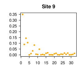
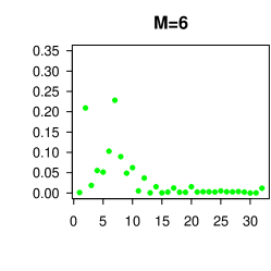
Figure 1: Comparison of probabilities of presence in raw data at site $i=9$ (left) and probabilities sampled from the Griffiths–Engen–McCloskey prior with $M=6$ (right). The $x$-axis represents species $j=1,\ldots,32$.

For an exhaustive description of the prior distribution on $\mathbf{p}$, the marginal description (3) needs be complemented by specifying a distribution for stochastic processes $(V_{j}(X),X\in\mathcal{X})$, for any positive integer $j$. Since (3) requires Beta marginals, natural candidates are Beta processes. A simple yet effective construct to obtain a Beta process is to transform a Gaussian process by the inverse cumulative distribution function ($\mathsf{CDF}$) transform as follows. Denote by $Z\sim\mathsf{N}(0,\sigma_{Z}^{2})$ a Gaussian random variable, by $\Phi_{\sigma_{Z}}$ its $\mathsf{CDF}$ and by $F_{M}$ a $\mathsf{Beta}(1,M)$ $\mathsf{CDF}$. Then $V=F_{M}^{-1}\circ\Phi_{\sigma_{Z}}(Z)$ is $\mathsf{Beta}(1,M)$ distributed, with $F_{M}^{-1}(U)=1-(1-U)^{1/M}$. Denote by $g_{\sigma_{Z},M}=F_{M}^{-1}\circ\Phi_{\sigma_{Z}}$. Note that the idea of including a transformed Gaussian process within a stick-breaking process is used in previous articles including Rodriguez et al., (2010); Rodriguez and Dunson, (2011); Barrientos et al., (2012); Pati et al., (2013).

In our case, we use Gaussian processes $\mathbf{\mathcal{Z}}_{j}$ on the space $\mathcal{X}$, $j=1,2,\ldots$, which define Beta processes $\mathbf{V}_{j}$, which in turn define the probabilities $\mathbf{p}_{j}$. Though the main parameters of interest are the $\mathbf{p}_{j}$, we will work hereafter with $\mathbf{\mathcal{Z}}_{j}$ for computational convenience.

The Gaussian process is used as a prior probability distribution over functions. It is fully specified by a mean function $m$, which we take equal to 0, and a covariance function $K$ defined by

$$K(X_{i},X_{l})=\mathsf{Cov}\big{(}\mathbf{\mathcal{Z}}_{j}(X_{i}),\mathbf{\mathcal{Z}}_{j}(X_{l})\big{)}.$$ (4)

We control the overall variance of $\mathbf{\mathcal{Z}}_{j}$ by a positive pre-factor $\sigma_{\mathbf{Z}}^{2}$ and write $K=\sigma_{\mathbf{Z}}^{2}\tilde{K}$ where $\tilde{K}$ is normalized in the sense that $\tilde{K}(X_{i},X_{i})=1$ for all $i$. We work with the squared exponential (SE), Ornstein–Uhlenbeck (OU), and rational quadratic (RQ) covariance functions. See Section S.2 in Supplementary Material for more details. All three involve a parameter $\lambda$ called the length-scale of the process $\mathbf{\mathcal{Z}}_{j}$. It tunes how far apart two points $X_{1}$ and $X_{2}$ have to be for the process to change significantly. The shorter $\lambda$ is, the rougher are the paths of the process $\mathbf{\mathcal{Z}}_{j}$. We adopt the same technique as van der Vaart and van Zanten, (2009) who deal with $\lambda$ by making it random with an inverse-Gamma (denoted $\mathsf{IG}$) prior distribution. They obtain adaptive minimax-optimal posterior contraction rates which indicate that the length-scale parameter $\lambda$ correctly adapts to the path smoothness. Gibbs, (1997) derived a covariance function where the length-scale $\lambda(X)$ is a (positive) function of $X$. This case is not studied here, although it could result in interesting behaviour, as noted in Rasmussen and Williams, (2006).

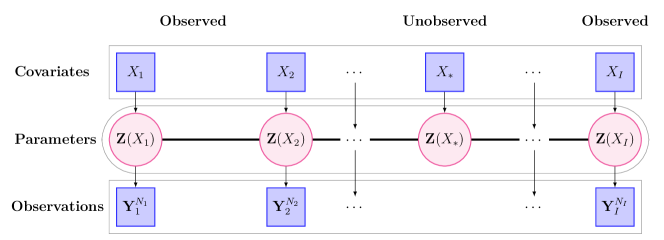
Figure 2: Diagram representation for the $\mathsf{Dep}$-$\mathsf{GEM}$ model. Squares represent observed data, i.e. covariates $\mathbf{X}=(X_{i})_{i=1,\ldots,I}$ and observations $\mathbf{Y}_{i}^{N_{i}}=(Y_{1,i},\ldots,Y_{N_{i},i})$, and circles represent parameters for the $\mathsf{Dep}$-$\mathsf{GEM}$ model.

Each species $j$ is associated to a Gaussian process $\mathbf{\mathcal{Z}}_{j}$. We have a set of $I$ points $\mathbf{X}=(X_{1},\ldots,X_{I})$ in the covariate space $\mathcal{X}$ which reduces the evaluation of the whole process $\mathbf{\mathcal{Z}}_{j}$ to its values at $\mathbf{X}$ denoted by $\mathbf{Z}_{j}=(Z_{1,j},\ldots,Z_{I,j})=(\mathbf{\mathcal{Z}}_{j}(X_{1}),\ldots,\mathbf{\mathcal{Z}}_{j}(X_{I}))$. We denote also by $\mathbf{Z}$ the matrix of all vectors $\mathbf{Z}_{j}$, $\mathbf{Z}=(Z_{ij})_{1\leq i\leq I,1\leq j\leq J}$. The vector $\mathbf{Z}_{j}$ is multivariate Gaussian. Its covariance matrix $K(\mathbf{X},\lambda,\sigma_{\mathbf{Z}})=(\sigma_{\mathbf{Z}}^{2}\tilde{K}_{\lambda}(X_{i},X_{l}))_{i,l=1,\ldots,I}$ is a Gram matrix with entries given by Equation (4). The prior distribution of $\mathbf{Z}_{j}$ is

$$\log\pi(\mathbf{Z}_{j}|\mathbf{X},\lambda,\sigma_{\mathbf{Z}})=\frac{1}{2}\mathbf{Z}_{j}^{\top}K^{-1}(\mathbf{X},\lambda,\sigma_{\mathbf{Z}})\mathbf{Z}_{j}-\frac{1}{2}\log|K(\mathbf{X},\lambda,\sigma_{\mathbf{Z}})|-\frac{I}{2}\log 2\pi,$$

or, written in terms of $\sigma_{\mathbf{Z}}^{2}$ and $\tilde{K}_{\lambda}=(\tilde{K}_{\lambda}(X_{i},X_{l}))_{i,l=1,\ldots,I}$,

$$\pi(\mathbf{Z}_{j}|\mathbf{X},\lambda,\sigma_{\mathbf{Z}})\propto\sigma_{\mathbf{Z}}^{-I}|\tilde{K}_{\lambda}|^{-1/2}\exp\Big{(}-\frac{\mathbf{Z}_{j}^{\top}\tilde{K}_{\lambda}^{-1}\mathbf{Z}_{j}}{2\sigma_{\mathbf{Z}}^{2}}\Big{)}.$$

The prior distribution is complemented by specifying the distributions over hyperparameters $\sigma_{\mathbf{Z}}$ the standard deviation, $\lambda$ the length-scale and $M$ the precision parameter of the $\mathsf{GEM}$ distribution. We use the following standard hyperpriors:

$$\sigma_{\mathbf{Z}}^{2}\sim\mathsf{IG}(a_{\mathbf{Z}},b_{\mathbf{Z}}),\,\,\lambda\sim\mathsf{IG}(a_{\lambda},b_{\lambda}),\text{ and }M\sim\mathsf{Ga}(a_{M},b_{M}).$$ (5)

Note that these are also common choices in the absence of dependence since they are conjugate priors, and recall that the inverse-Gamma for $\lambda$ also proves to lead to good convergence results.

It is convenient to estimate the model in terms of $\mathbf{Z}_{j}$, and then to use the transform $\mathbf{V}_{j}=g_{\sigma_{\mathbf{Z}},M}(\mathbf{Z}_{j})$. The likelihood is

$$\mathcal{L}(\mathbf{Y}|\mathbf{Z},\mathbf{X},\sigma_{\mathbf{Z}},M)=\prod_{j=1}^{J}\prod_{i=1}^{I}g_{\sigma_{\mathbf{Z}},M}(Z_{j}(X_{i}))^{N_{ij}}(1-g_{\sigma_{\mathbf{Z}},M}(Z_{j}(X_{i})))^{\bar{N}_{i,j+1}},$$ (6)

where $\bar{N}_{i,j+1}=\sum_{l>j}{N_{il}}$. The posterior distribution is then

$$\pi(\mathbf{Z},\lambda,\sigma_{\mathbf{Z}},M|\mathbf{Y},\mathbf{X})\propto\mathcal{L}(\mathbf{Y}|\mathbf{Z},\mathbf{X},\sigma_{\mathbf{Z}},M)\pi(\mathbf{Z}|\mathbf{X},\lambda,\sigma_{\mathbf{Z}})\pi(\sigma_{\mathbf{Z}})\pi(\lambda)\pi(M).$$ (7)

3.3 Posterior computation and inference

Here we highlight the main points of interest of the algorithm which is fairly standard, whereas the fully detailed posterior sampling procedure can be found in Supplementary Material, Section S.1. Inference in the $\mathsf{Dep}$-$\mathsf{GEM}$ model is performed via two distinct samplers: (i) first a Markov chain Monte Carlo (hereafter $\mathsf{MCMC}$) algorithm comprising Gibbs and Metropolis-Hastings steps for sampling the posterior distribution of $(\mathbf{Z},\sigma_{\mathbf{Z}},\lambda,M)$. It proceeds by sequentially updating each parameter $\mathbf{Z},\,\sigma_{\mathbf{Z}},\,\lambda$ and $M$ via its conditional distribution; (ii) second a sampler from the posterior predictive distribution of $\mathbf{Z}_{*}$. This consists in posterior conditional sampling of the Gaussian process $\mathbf{\mathcal{Z}}$ at covariates $\mathbf{X}_{*}=(X_{1}^{*},\ldots,X_{I_{*}}^{*})$ which are not observed, i.e. such that $\{X_{1},\ldots,X_{I}\}$ and $\{X_{1}^{*},\ldots,X_{I_{*}}^{*}\}$ are pairwise distinct. This is achieved by integrating out $\mathbf{Z}$ in the conditional distribution of $\mathbf{Z}_{*}$ given $\mathbf{Z}$ according to the posterior distribution sampled in (i).

3.4 Distributional properties

We provide in Proposition 1 the first prior moments, expectation, variance and covariance, of the diversity. It is of crucial importance in order to elicit the values of hyperparameters, or their prior distribution, based on prior information (expert, etc.) Additionally, since the $\mathsf{Dep}$-$\mathsf{GEM}$ introduces some dependence across the $p_{j}(X_{i})$ in varying $X_{i}$, the question of the dependence induced in a diversity index arises. Denote the Simpson index by $H_{\mathsf{\scriptstyle Simp}}(X_{i})$, see Section 2.3. An answer is formulated in the next Proposition in terms of the covariance between $H_{\mathsf{\scriptstyle Simp}}(X_{1})$ and $H_{\mathsf{\scriptstyle Simp}}(X_{2})$. Further properties worth mentioning are presented in Supplementary Material Section S.3, including marginal moments of the $\mathsf{Dep}$-$\mathsf{GEM}$ prior and continuity of sample paths in Proposition 2, full support in Proposition 4, a study of the joint distribution of samples from the $\mathsf{Dep}$-$\mathsf{GEM}$ prior in Proposition 5, and a discussion on the joint exchangeable partition probability function based on size-biased permutations in Section S.3.4.

Proposition 1

The expectation and variance of the Simpson diversity, and its covariance at two sites $X_{1}$ and $X_{2}$, induced by the $\mathsf{Dep}$-$\mathsf{GEM}$ distribution, are as follows

$$\mathsf{E}(H_{\mathsf{\scriptstyle Simp}})=\frac{M}{1+M},\,\mathsf{Var}(H_{\mathsf{\scriptstyle Simp}}(X))\frac{2M}{(M+1)(M+1)_{3}},$$ (8)

$$\mathsf{Cov}(H_{\mathsf{\scriptstyle Simp}}(X_{1}),H_{\mathsf{\scriptstyle Simp}}(X_{2}))=\frac{\nu_{2,2}(1-\omega_{2,0})+2\nu_{2,0}\gamma_{2,2}}{(1-\omega_{2,0})(1-\omega_{2,2})}-\nu_{1,0}^{2},$$ (9)

where $\nu_{i,j}=\mathsf{E}[V^{i}(X_{1})V^{j}(X_{2})]$, $\omega_{i,j}=\mathsf{E}[(1-V(X_{1}))^{i}(1-V(X_{2}))^{j}]$, and $\gamma_{i,j}=\mathsf{E}[V^{i}(X_{1})(1-V(X_{2}))^{j}]$.

The values of $\nu_{i,j},\omega_{i,j},\gamma_{i,j}$ cannot be computed in a closed-form expression when $i\times j\neq 0$ but they can be approximated numerically. The same formal computations for the Shannon index lead to somehow more complex expressions which are not displayed here (see also Cerquetti,, 2014). The expressions of Proposition 1 are illustrated on Figure 3.

The precision parameter $M$ has the following impact on the prior distribution and on the diversity: when $M\rightarrow 0$, the prior degenerates to a single species with probability 1, hence $H_{\mathsf{\scriptstyle Simp}}\rightarrow 0$, whereas when $M\rightarrow\infty$, the prior tends to favour infinitely many species, and $H_{\mathsf{\scriptstyle Simp}}\rightarrow 1$. In both cases, the variance and the covariance vanish. In between, the variance is maximum for $M\approx 0.49$. The covariance at $X_{1}$ and $X_{2}$ equals the variance when $X_{1}=X_{2}$ (by continuity of the sample paths), while the covariance vanishes when $|X_{1}-X_{2}|\rightarrow\infty$ (this corresponds to independence for infinitely distant covariates).

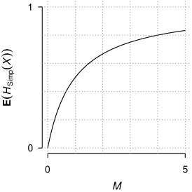
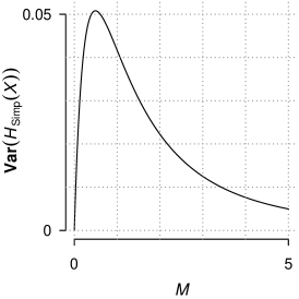
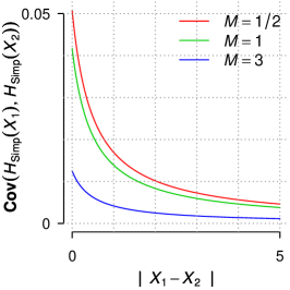
Figure 3: Illustration of Proposition 1. Left: $\mathsf{E}(H_{\mathsf{\scriptstyle Simp}}(X))$ w.r.t. $M$. Middle: $\mathsf{Var}(H_{\mathsf{\scriptstyle Simp}}(X))$ w.r.t. $M$. Right: three paths of $\mathsf{Cov}(H_{\mathsf{\scriptstyle Simp}}(X_{1}),H_{\mathsf{\scriptstyle Simp}}(X_{2}))$ w.r.t. $|X_{1}-X_{2}|$ for $M\in\{1/2,1,3\}$.

Despite the fact that the first moments of the diversity indices under a $\mathsf{GEM}$ prior can be derived, a full description of the distribution seems hard to achieve. For instance, the distribution of the Simpson index involves the small-ball like probabilities $\mathsf{P}(\sum_{j}p_{j}^{2}<a)$ for which, to the best of our knowledge, no result is known under the $\mathsf{GEM}$ distribution.

4 Case study results

We now apply the model to the estimation of diversity and of effective concentrations $EC_{x}$ as described in Section 2, and assess the goodness of fit of the model and its sensitivity to sampling variation.

4.1 Results

The $\mathsf{MCMC}$ algorithm is run with squared exponential Gaussian processes for 50,000 iterations thinned by a factor of 5 with a burn-in of 10,000 iterations. The parameters of the hyperpriors (5) are $a_{\mathbf{Z}}=b_{\mathbf{Z}}=1$, $\eta_{\lambda}=1$, $a_{\lambda}=b_{\lambda}=1$ and $a_{M}=b_{M}=1$. The efficiency and convergence of the $\mathsf{MCMC}$ sampler was assessed by trace plots and autocorrelations of the parameters.

The results for the Simpson diversity estimation are illustrated in Figure 4 for the $\mathsf{Dep}$-$\mathsf{GEM}$ model (left, 4) and for the independent $\mathsf{GEM}$ model (right, 4). The horizontal axis represents the pollution level TPH and the vertical axis represents the Simpson diversity. The posterior mean of the diversity is represented by the solid line, and a 95% credible interval is indicated by dashed lines, for the dependent model only. The dots indicate the empirical estimator of the diversity.

The $\mathsf{Dep}$-$\mathsf{GEM}$ model (Figure 4) suggested that diversity first increases with TPH with a maximum at 4,000mg TPH/kg soil, and then decreases with TPH. The $\mathsf{GEM}$ model estimates are shown for comparison in Figure 4. These estimates showed more variability with respect to TPH in that they are closer to the empirical estimates of the diversity. Note that the $\mathsf{GEM}$ estimates were only available at levels of the covariate that were present in the data, because of the independent nature of the model specification. The $\mathsf{Dep}$-$\mathsf{GEM}$, in contrast, provided predictions across the full range of TPH values. The credible bands are narrowest for TPH between 3,000-5,000mg TPH/kg soil, due to borrowing of information between concentrated points, and they widen both at TPH = 0, due to a lot of data points with high variability, and at large TPH, due to few data points.

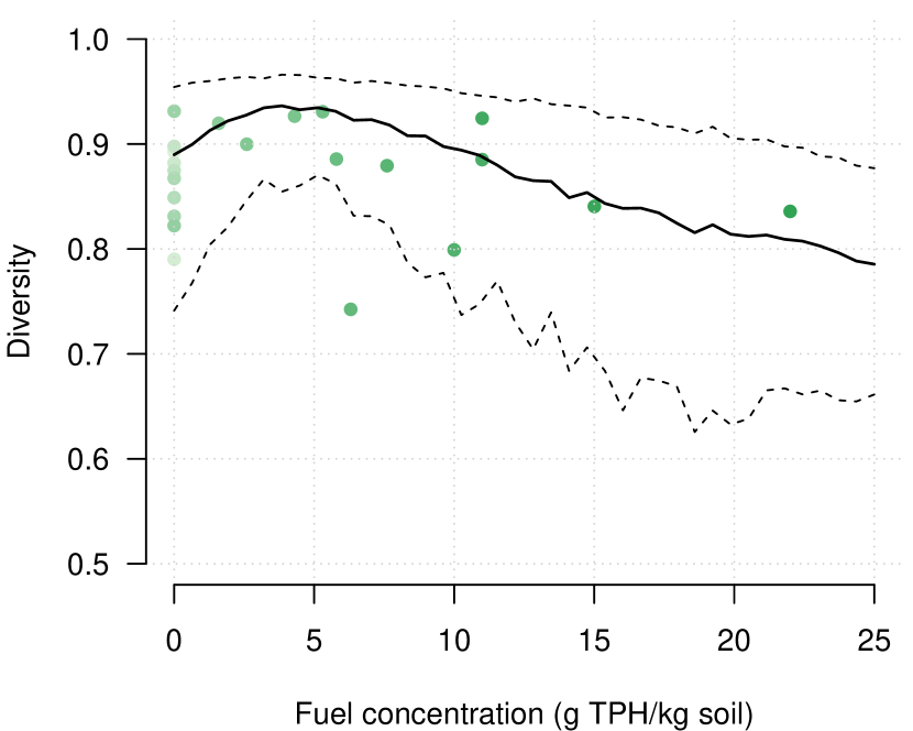
(a) $\mathsf{Dep}$-$\mathsf{GEM}$

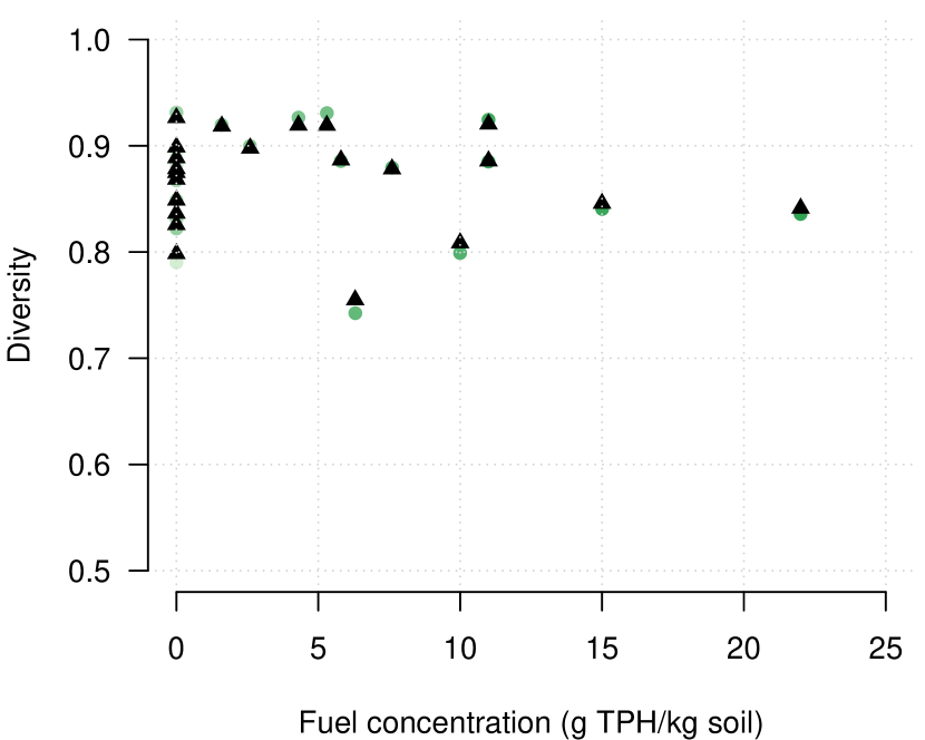
(b) Independent $\mathsf{GEM}$

Figure 4: Diversity estimation results. (a) $\mathsf{Dep}$-$\mathsf{GEM}$ model estimates (50,000 MCMC samples). Solid line: Simpson diversity estimate. Dashed lines: 95$\%$ credible interval for the Simpson diversity. Dots: Empirical estimates of Simpson diversity. (b) Independent $\mathsf{GEM}$ model estimates (50,000 MCMC samples). Triangles: posterior mean estimate of the Simpson diversity.

The Jaccard dissimilarity curve with respect to TPH is shown in Figure 5. The $EC_{x}$ values are estimated as explained in Section 2.4 and provided in Table 5. Dissimilarity increased with TPH, illustrating that the contaminant alters community structure. Typically, $EC_{10}$, $EC_{20}$ and $EC_{50}$ values of Table 5 are reported in toxicity studies to be used in the derivation of protective concentrations in environmental guidelines, see Section 2.4. $EC_{10}$, $EC_{20}$ and $EC_{50}$ values estimated from this model are 1,250, 1,875 and 5,000 mg TPH/kg soil respectively. For small $x$ (less than 10%), the lower bound of the credible interval on the $EC_{x}$ value is zero, because both TPH and dissimilarity values are bounded below by zero. Conversely, for large $x$ (more than 75%), the upper bound on the credible interval is 25,000, which is the limit of the TPH range in our analysis.

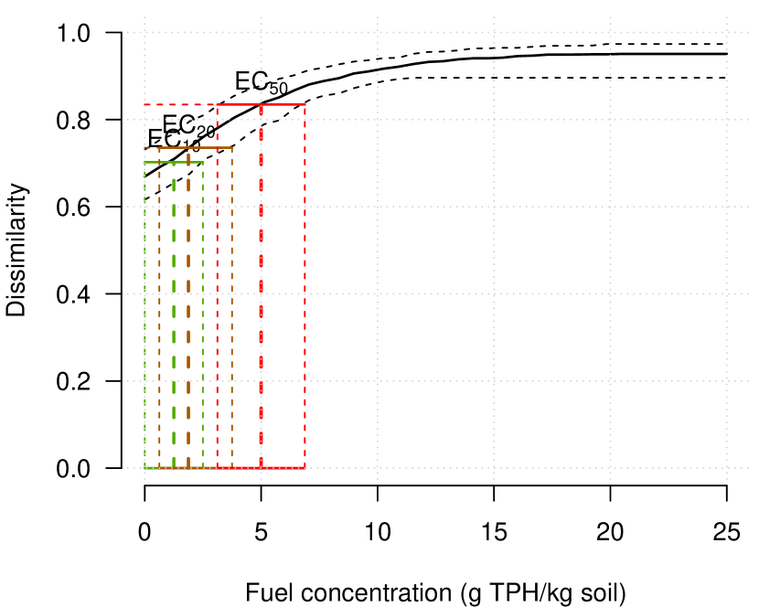
(a) Illustration of $EC_{x}$ and Jaccard dissimilarity

$x$	$EC_{x}$	min	max
10	1250	0	2500
20	1875	625	3750
50	5000	3125	6875

(b) $EC_{x}$ estimates and 95% credible intervals (min, max)

Figure 5: Jaccard dissimilarity and $EC_{x}$ estimation results. (a) Posterior distribution ($\mathsf{Dep}$-$\mathsf{GEM}$ model) of Jaccard dissimilarity between the control community, where TPH equals zero, and communities where TPH$>0$. Solid line: mean estimate Dashed lines: 95% credible intervals of the dissimilarity estimate. Color: Illustration of estimation of $EC_{x}$ values and their credible intervals. (b) Estimates of $EC_{x}$ values and their credible intervals.

4.2 Posterior predictive checks

Since we aim at comparing the performance of the model in terms of diversity estimates, we also need to specify measures of goodness of fit. We resort to the conditional predictive ordinates (CPOs) statistics, which are now widely used in several contexts for model assessment. See, for example, Gelfand, (1996). For each species $j$, the CPO statistic is defined as follows:

$$\operatorname{CPO}_{j}=\mathcal{L}(\mathbf{Y}_{j}|\mathbf{Y}_{-j})=\int\mathcal{L}(\mathbf{Y}_{j}|\theta)\pi(\mbox{d}\theta|\mathbf{Y}_{-j})$$

where $\mathcal{L}$ represents the likelihood (6), $\mathbf{Y}_{-j}$ denotes data for species $j$ over all sites, $\mathbf{Y}_{-j}$ denotes the observed sample $\mathbf{Y}$ with the $j$-th species excluded and $\pi(\mbox{d}\theta|\mathbf{Y}_{-j})$ is the posterior distribution of the model parameters $\theta=(\mathbf{Z},\sigma_{\mathbf{Z}},\lambda,M)$ based on data $\mathbf{Y}_{-j}$. By rewriting the statistic $\operatorname{CPO}_{j}$ as

$$\operatorname{CPO}_{j}=\biggl{(}\int\big{(}\mathcal{L}(\mathbf{Y}_{j}|\theta)\big{)}^{-1}\pi(\mbox{d}\theta|\mathbf{Y})\biggr{)}^{-1},$$

it can be easily approximated by Monte Carlo as

$$\widehat{\operatorname{CPO}_{j}}=\Biggl{(}\frac{1}{T}\sum_{t=1}^{T}\big{(}\mathcal{L}(\mathbf{Y}_{j}|\theta^{(t)})\big{)}^{-1}\Biggr{)}^{-1},$$

where $\{\theta^{(t)},t=1,2,\ldots,T\}$ is an MCMC sample from $\pi(\mbox{d}\theta|\mathbf{Y})$. We illustrate the logarithm of the $\operatorname{CPO}_{j}$, $j=1,\ldots,J$, by boxplots in Figure 6, and summarize their values in Table 6 in two ways, as an average of the logarithm of CPOs and as the median of the logarithm of CPOs. For the purpose of the comparison, we have estimated six models. The first three are the $\mathsf{Dep}$-$\mathsf{GEM}$ model with squared-exponential (SE), Ornstein-Uhlenbeck (OU) and rational quadratic (RQ) covariance functions, see Section S.2 in Supplementary Material. The fourth is the probit stick-breaking process (PSBP) by Rodriguez and Dunson, (2011). For the purpose of comparison, we have set the hyperparameters of the $\mathsf{PSBP}$ so as to match the expected number of clusters of the $\mathsf{Dep}$-$\mathsf{GEM}$ prior. Last, we used two variants of the $\mathsf{GEM}$ prior: first independent $\mathsf{GEM}$ priors at each site, as in Figure 4, and second a single $\mathsf{GEM}$ prior where the presence probabilities are all drawn from the same $\mathsf{GEM}$ distribution.

The single $\mathsf{GEM}$ is used as a very crude baseline (it is not shown in the boxplots) which does poorly compared to the five other models. As expected, the dependence induced by the $\mathsf{Dep}$-$\mathsf{GEM}$ and the $\mathsf{PSBP}$ greatly improves the predictive quality of the model as shows the comparison to the independent $\mathsf{GEM}$. The $\mathsf{Dep}$-$\mathsf{GEM}$ model has a slightly better predictive fit than the $\mathsf{PSBP}$ which seems to indicate that the total ordering of the species that we use helps as far as prediction is concerned.

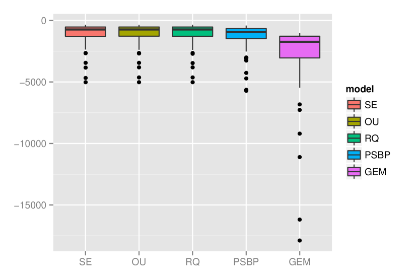
(a)

Model	Mean.CPO	Median.CPO
Dep-GEM SE	-1131.3	-732.9
Dep-GEM OU	-1131.5	-732.7
Dep-GEM RQ	-1131.8	-731.4
PSBP	-1373.5	-932.3
Independent GEM	-2910.1	-1734.1
Single GEM	-34606.2	-28773.6

(b)

Figure 6: Log-conditional predictive ordinates (log-CPO) for different models and prior specifications (see text). (a) Boxplots of log-CPO. (b) Summaries of log-CPO, mean and median.

4.3 Sensitivity to sampling variation

A thorough sensitivity analysis to sampling variation was conducted in Arbel et al., 2015b . It consisted in estimating the model on modified data, by (i) deleting the least abundant species; (ii) including additional species; (iii) excluding sites randomly. This sensitivity analysis showed that the model provides consistent results with data modified as described, thus supporting some robustness to sampling variation.

5 Model considerations and extensions

In addition to looking at a sensitivity analysis to sampling variation as in Section 4.3, here we consider sensitivity with respect to the model itself which could be extended in a number of ways.

5.1 Imperfect detection

As pointed out in Section 2.3 we do not connect our model to the fields of occupancy modeling and imperfect detection developed for instance by Royle and Dorazio, (2008). A possible extension to the current model is by accounting for imperfect detection. Following Royle and Dorazio, (2006); Dorazio et al., (2008), a simple yet effective way to handle this extension is to define a probability of detection $\theta_{i}$ fixed for each site $i$, and to model the variability of $\theta_{i}$ across $i$ by an exchangeable prior. Since $\theta_{i}$ affects each species by the same relative proportion, the probabilities of presence $p_{j}(X_{i})$ are invariant to such a formulation, and so is the diversity. Diversity being the prime focus of the present paper, we argue that there is no need to account for imperfect detection in our model, though it could be easily extended as briefly sketched if interest deviates from diversity.

5.2 Assumption on data, stochastic decrease of the $\hat{p}_{j}$’s

We have assumed that after ordering with respect to overall abundance, the $\hat{p}_{j}$’s display a stochastically decreasing pattern as in Figure 1. In our experience, this assumption turns out to be satisfied with most of species data sets, where species can be microbes, animals, words in text, DNA sequences, etc. However, this assumption proves to be overly restrictive in the following cases i) data might be subject to detection error: this is covered in the previous section by changing the prior adequately; ii) there are outlier species which contradict the assumption: this could be addressed by adding a mixture layer in the prior specification; iii) the underlying assumption itself is not true: this is for instance the case when all species are overall evenly distributed. A treatment would be context specific and depend on the field.

5.3 Comparison to other models

In Section 4 we have compared the $\mathsf{Dep}$-$\mathsf{GEM}$ model to other models: two $\mathsf{GEM}$ priors and the probit stick-breaking prior ($\mathsf{PSBP}$) of Rodriguez and Dunson, (2011). The benefits of the $\mathsf{Dep}$-$\mathsf{GEM}$ over the first two is apparent in terms of smoothing of the estimates due to the a priori dependence, see Figure 4. It also carries over better predictive fit, see Figure 6 and Table 6, and most importantly allows us to assess the response of species to any value of the contaminant, including unsampled values. With respect to the $\mathsf{PSBP}$, the CPO indicate a slightly better predictive fit of the $\mathsf{Dep}$-$\mathsf{GEM}$ prior, at least for the case study at hand.

6 Discussion

We have presented a Bayesian nonparametric dependent model for species data, based on the distribution of the weights of a Dependent Dirichlet process, named $\mathsf{Dep}$-$\mathsf{GEM}$ distribution, which is constructed thanks to Gaussian processes. A fundamental advantage of our approach based on the stick-breaking is that it brings considerable flexibility when it comes to defining the dependence structure. It is defined by the kernel of a Gaussian process, whose flexibility allows learning the different features of dependence in the data.

In terms of model fit, we have shown that the $\mathsf{Dep}$-$\mathsf{GEM}$ model improves estimation compared to an independent $\mathsf{GEM}$ model. This was conducted by computing conditional predictive ordinates (CPOs). In addition, our dependent model allows predictions at arbitrary covariate level (not just those that were in the data). It allows, for example, estimation of the diversity and the dissimilarity across the full range of covariates. This is an essential feature in applications where the experimental data are sparse and is instrumental in estimating the $EC_{x}$ values.

There are computational limitations to the use of this model. The estimation can deal with large number of observations since the complexity grows linearly with the number of different observed species $J$. However the number of unique covariate values $I$ represents the limiting factor of the algorithm, and may lead to dimensionality problems. One could consider the use of $\mathsf{INLA}$ approximations (see Rue et al.,, 2009) in the case of prohibitively large $I$.

Possible extensions of the present paper include the following. First, extra flexibility would be guaranteed by using the two-parameter Poisson-Dirichlet distribution instead of the $\mathsf{GEM}$ distribution, since it controls more effectively the posterior distribution of the number of clusters (Lijoi et al.,, 2007). This can be done at almost no extra cost, since it only requires one additional step in the Gibbs sampler. Second, the $\mathsf{Dep}$-$\mathsf{GEM}$ model is tested on univariate variables only, but could be extended to multivariate variables, i.e., $X\in\mathbb{R}^{d}$, $d>1$. Instead of a Gaussian process $\mathbf{\mathcal{Z}}$, one would use a Gaussian random field $\mathbf{\mathcal{Z}}^{d}$. To that purpose, all the methodology presented in Section 3 remains valid. The algorithm can become computationnally challenging in the case of large dimensional covariates but it does not carry additional difficulty for limited dimension. Applications of such an extension are promising, such as testing joint effects in dynamical models (time $\times$ contaminant), in spatial models (position $\times$ contaminant), etc.

The supplementary material contains details about posterior computation and inference in the $\mathsf{Dep}$-$\mathsf{GEM}$ model, additional results and omitted proofs that complement the analysis of the main text.

S.1 Posterior computation and inference in the $\mathsf{Dep}$-$\mathsf{GEM}$ model

Here we describe how to design a Markov chain Monte Carlo ($\mathsf{MCMC}$) algorithm for sampling the posterior distribution of $(\mathbf{Z},\sigma_{\mathbf{Z}},\lambda,M)$ in the $\mathsf{Dep}$-$\mathsf{GEM}$ model. Up to a transformation, it is equivalent to sample the parameters in terms of Gaussian vectors $\mathbf{Z}$ or Beta breaks $\mathbf{V}$. We denote by $\pi$ the prior distribution. We make use of the factorized form of the likelihood in Equation (6) in the main paper in order to break the posterior sampling into $J=\max_{i}J_{i}$ independent sampling schemes. It remains a multivariate sampling scheme in terms of the $I$ sites, but avoids a very high dimensional scheme of size $I\times J$.

S.1.1 $\mathsf{MCMC}$ algorithm

We use an $\mathsf{MCMC}$ algorithm comprising Gibbs and Metropolis-Hastings steps for sampling the posterior distribution of $(\mathbf{Z},\sigma_{\mathbf{Z}},\lambda,M)$, which proceeds by sequentially updating each of the parameters $\mathbf{Z},\,\sigma_{\mathbf{Z}},\,\lambda$ and $M$ via its conditional distribution as described in Algorithm 1 (general sampler) and Algorithm 2 (Metropolis-Hastings step for a generic parameter $\boldsymbol{\theta}$). Denote by $P_{\boldsymbol{\theta}}(\,\cdot\,)$ the target distribution (full conditional), and by $Q_{\boldsymbol{\theta}}(\,\cdot\,\,|\,\boldsymbol{\theta})$ the proposal for a generic parameter $\boldsymbol{\theta}$. The variance of the latter proposal, denoted by $\sigma^{2}_{Q_{\boldsymbol{\theta}}}$, is tuned during a burn-in period.
Algorithm 1 $\mathsf{Dep}$-$\mathsf{GEM}$ • Update $\mathbf{Z}$ given $(\sigma_{\mathbf{Z}},\lambda,M)$ • Update $\sigma_{\mathbf{Z}}$ given $(\mathbf{Z},\lambda,M)$ • Update $\lambda$ given $(\mathbf{Z},\sigma_{\mathbf{Z}},M)$ • Update $M$ given $(\mathbf{Z},\sigma_{\mathbf{Z}},\lambda)$ Algorithm 2 Metropolis-Hastings step • Given $\boldsymbol{\theta}$, propose $\boldsymbol{\theta}^{\prime}\sim Q_{\boldsymbol{\theta}}(\,\cdot\,\,|\,\boldsymbol{\theta})$ • Compute $\rho_{\boldsymbol{\theta}}=\frac{P_{\boldsymbol{\theta}}(\boldsymbol{\theta}^{\prime})}{P_{\boldsymbol{\theta}}(\boldsymbol{\theta})}\frac{Q_{\boldsymbol{\theta}}(\boldsymbol{\theta}|\boldsymbol{\theta}^{\prime})}{Q_{\boldsymbol{\theta}}(\boldsymbol{\theta}^{\prime}\,|\,\boldsymbol{\theta})}$ • Accept $\boldsymbol{\theta}^{\prime}$ wp $\min(\rho_{\boldsymbol{\theta}},1)$, otherwise keep $\boldsymbol{\theta}$

The full conditionals and target distributions are now fully described:

1. Conditional for $\mathbf{Z}$: Metropolis algorithm with Gaussian jumps proposal $\mathbf{Z}^{\prime}\sim Q_{\mathbf{Z}}(\,\cdot\,|\,\mathbf{Z})=\mathsf{N}_{I}(\mathbf{Z},\sigma_{Q_{\mathbf{Z}}}^{2}\tilde{K}_{\lambda})$. We use a covariance matrix proportional to the prior covariance matrix $\tilde{K}_{\lambda}$, which leads to improved convergence of the algorithm compared to the use of a homoscedastic alternative. The target distribution is

   $$P_{\mathbf{Z}}(\mathbf{Z})\propto\mathcal{L}(\mathbf{Y}|\mathbf{Z},\mathbf{X},\sigma_{\mathbf{Z}},M)\allowbreak\pi(\mathbf{Z}|\mathbf{X},K(\mathbf{X},\lambda,\sigma_{\mathbf{Z}})).$$

2. Conditional for $\sigma_{\mathbf{Z}}$: Metropolis-Hastings algorithm with a Gaussian proposal left truncated to 0, ${\sigma^{\prime}_{\mathbf{Z}}}\sim Q_{{\sigma_{\mathbf{Z}}}}(\,\cdot\,|\,{\sigma_{\mathbf{Z}}})=\mathsf{N}_{\mathsf{\scriptstyle 0-trunc}}({\sigma_{\mathbf{Z}}},\sigma_{Q_{{\sigma_{\mathbf{Z}}}}}^{2})$, and target distribution

   $$P_{\sigma_{\mathbf{Z}}}(\sigma_{\mathbf{Z}})\propto\mathcal{L}(\mathbf{Y}|\mathbf{Z},\mathbf{X},\sigma_{\mathbf{Z}},M)\sigma_{\mathbf{Z}}^{-I-a_{\mathbf{Z}}/2}\exp\Big{(}-\frac{\mathbf{Z}^{\top}\tilde{K}_{\lambda}^{-1}\mathbf{Z}-2b_{\mathbf{Z}}}{2\sigma_{\mathbf{Z}}^{2}}\Big{)}.$$

3. Conditional for $\lambda$: Metropolis-Hastings algorithm with a Gaussian proposal left truncated to 0, $\lambda^{\prime}\sim Q_{\lambda}(\,\cdot\,|\,\lambda)=\mathsf{N}_{\mathsf{\scriptstyle 0-trunc}}(\lambda,\sigma_{Q_{\lambda}}^{2})$, and target distribution

   $$P_{\lambda}(\lambda)\propto\pi(\mathbf{Z}|\mathbf{X},K(\mathbf{X},\lambda,\sigma_{\mathbf{Z}}))\pi(\lambda).$$

4. Conditional for $M$: Metropolis algorithm with a Gaussian proposal left truncated to 0, $M^{\prime}\sim Q_{M}(\,\cdot\,|\,M)=\mathsf{N}_{\mathsf{\scriptstyle 0-trunc}}(M,\sigma_{Q_{M}}^{2})$, and target distribution

   $$P_{M}(M)\propto M^{A_{M}-1}\exp(-b_{M}M)\prod_{i=1}^{I}g_{\sigma_{\mathbf{Z}},M}(Z_{i})^{N_{ij}}(1-g_{\sigma_{\mathbf{Z}},M}(Z_{i}))^{\bar{N}_{i,j+1}}.$$

Remark 1

The dimensionality of the $\mathsf{MCMC}$ algorithm described above equals the number of covariates $I$ (or blocks of covariates). Large dimensions can be an obstacle to the use of traditional methods (mainly due to matrix inversion). A direction that has not been investigated could be to replace $\mathsf{MCMC}$ algorithms with faster approximations, of the type of $\mathsf{INLA}$ for example, see Rue et al., (2009).

S.1.2 Predictive distribution

Up to now we have considered the vector $\mathbf{Z}$, which is the evaluation of the Gaussian process $\mathbf{\mathcal{Z}}$ at the observed covariates $\mathbf{X}=(X_{1},\ldots,X_{I})$. We are now interested in new outputs, called test outputs, $\mathbf{Z}_{*}$, associated with test covariates $\mathbf{X}_{*}=(X_{1}^{*},\ldots,X_{I_{*}}^{*})$ which are not observed, i.e. $\{X_{1},\ldots,X_{I}\}$ and $\{X_{1}^{*},\ldots,X_{I_{*}}^{*}\}$ are pairwise distinct. An appealing feature of the use of Gaussian processes is the possibility to easily derive the predictive distribution of $\mathbf{Z}_{*}$, which is achieved as follows. The joint distribution of the vector outputs $(\mathbf{Z},\mathbf{Z}_{*})$ according to the prior is the following $I+I_{*}$ multivariate Gaussian distribution

$$\bigg{(}\begin{matrix}\,\mathbf{Z}_{\phantom{*}}\\ \,\mathbf{Z}_{*}\end{matrix}\bigg{)}\sim\mathsf{N}_{I+I_{*}}\bigg{[}\boldsymbol{0},\bigg{(}\begin{matrix}K(\mathbf{X},\mathbf{X})&K(\mathbf{X},\mathbf{X}_{*})\\ K(\mathbf{X}_{*},\mathbf{X})&K(\mathbf{X}_{*},\mathbf{X}_{*})\end{matrix}\bigg{)}\bigg{]},$$ (S.1)

where the covariance matrices $K(\mathbf{X},\mathbf{X})$, $K(\mathbf{X},\mathbf{X}_{*})=K(\mathbf{X}_{*},\mathbf{X})^{\top}$ and $K(\mathbf{X}_{*},\mathbf{X}_{*})$ (resp. $I\times I$, $I\times I_{*}$ and $I_{*}\times I_{*}$ matrices) are defined by their entries according to the choice of the Gaussian process. The conditional density of $\mathbf{Z}_{*}$ given $\mathbf{Z}$ is the following Gaussian distribution (see Rasmussen and Williams,, 2006):

$$\mathbf{Z}_{*}\,|\,\mathbf{X}_{*},\mathbf{X},\mathbf{Z}\sim\mathsf{N}_{I_{*}}(m_{*}(\mathbf{Z}),K_{*}),\text{ with }m_{*}(\mathbf{Z})=K(\mathbf{X}_{*},\mathbf{X})K(\mathbf{X},\mathbf{X})^{-1}\mathbf{Z},$$ (S.2)

$$\text{ and }K_{*}=K(\mathbf{X}_{*},\mathbf{X}_{*})-K(\mathbf{X}_{*},\mathbf{X})K(\mathbf{X},\mathbf{X})^{-1}K(\mathbf{X},\mathbf{X}_{*}).$$

The predictive distribution of $\mathbf{Z}_{*}$ is obtained by integrating out $\mathbf{Z}$ in the conditional distribution (S.2) according to the posterior distribution $\pi(\mathbf{Z}|\mathbf{Y},\mathbf{X})$:

$$\pi(\mathbf{Z}_{*}\,|\,\mathbf{X}_{*},\mathbf{Y})=\int\pi(\mathbf{Z}_{*}\,|\,\mathbf{X}_{*},\mathbf{X},\mathbf{Z})\pi(\mathbf{Z}|\mathbf{Y},\mathbf{X})\mbox{d}\mathbf{Z}.$$ (S.3)

Simulating from a predictive distribution of the form of (S.3) is described in Algorithm 3. Once a sample of $\mathbf{Z}$ from the posterior distribution $\pi(\mathbf{Z}|\mathbf{Y},\mathbf{X})$ is available, one obtains a sample from the predictive distribution at almost no extra cost, by sampling from the multivariate normal distribution (S.2). One matrix, $K(\mathbf{X},\mathbf{X})$, has to be inverted, but that computation is already done for the $\mathsf{MCMC}$ sampler. The variance $K_{*}$ of (S.2) is to be computed once. Then it is efficient to draw a sample of the desired size from the centred normal $\mathsf{N}(0,K_{*})$, and then add the means $m_{*}(\mathbf{Z})$ for $\mathbf{Z}$ in the posterior sample. We can obtain the predictive distribution of any $\mathbf{Z}_{*}$ associated with any test covariates $\mathbf{X}_{*}$, hence allowing prediction in the whole space $\mathcal{X}$.

Algorithm 3 Predictive distribution simulation

• Sample $\mathbf{Z}$ from the posterior distribution $\pi(\mathbf{Z}|\mathbf{Y},\mathbf{X})$

• Given $\mathbf{Z}$, sample $\mathbf{Z}_{*}$ from the conditional distribution $\pi(\mathbf{Z}_{*}\,|\,\mathbf{X}_{*},\mathbf{X},\mathbf{Z})$

S.2 Covariance matrices

We work with the squared exponential (SE), Ornstein–Uhlenbeck (OU), and rational quadratic (RQ) covariance functions. The next table provides the normalized covariance function $\tilde{K}(X_{1},X_{2})=\tilde{K}_{\lambda}(X_{1},X_{2})$ for these three options.

Covariance function	$\tilde{K}_{\lambda}(X_{1},X_{2})$
Squared exponential (SE)	$\exp\big{(}-(X_{1}-X_{2})^{2}/(2\lambda^{2})\big{)}$
Ornstein–Uhlenbeck (OU)	$\exp\big{(}-|X_{1}-X_{2}|/\lambda\big{)}$
Rational quadratic (RQ)	$\big{(}1+(X_{1}-X_{2})^{2}/(2\lambda^{2})\big{)}^{-1}$

S.3 Distributional properties

The purpose of this section is to present key distributional properties of the $\mathsf{Dep}$-$\mathsf{GEM}$ prior in terms of (i) moments and continuity, (ii) full support, (iii) dependence and (iv) size-biased permutations. Proofs are deferred to Section S.4.

S.3.1 Marginal moments and continuity

We start by proving the continuity of sample-paths of the process $\mathbf{p}\sim$$\mathsf{Dep}$-$\mathsf{GEM}$ $(M)$ and providing its marginal moments.

Proposition 2

Let $\mathbf{p}\sim$$\mathsf{Dep}$-$\mathsf{GEM}$ $(M)$. Then $\mathbf{p}$ is stationary and marginally, $\mathbf{p}\sim\mathsf{GEM}(M)$. Also, $\mathbf{p}$ has continuous paths (i.e. $X\rightarrow(p_{1}(X),p_{2}(X),\ldots)$ is continuous for the sup norm), and its marginal moments are

$$\mathsf{E}(p_{j}(X))=\frac{M^{j-1}}{(M+1)^{j}},\quad\mathsf{E}(p_{j}^{n}(X))=\frac{n!}{M_{(n)}}\left(\frac{M}{M+n}\right)^{j},$$

$$\mathsf{Var}(p_{j}(X))=\frac{2M^{j-1}}{(M+1)(M+2)^{j}}-\frac{M^{2(j-1)}}{(M+1)^{2j}},$$

$$\mathsf{Cov}(p_{j}(X),p_{k}(X))=\frac{M^{(j\vee k)-1}}{(M+1)^{|j-k|+1}(M+2)^{j\wedge k}}-\frac{M^{j+k-2}}{(M+1)^{j+k}},\,k\neq j,$$

for any $j,k\geq 1$, $n\geq 0$, and where $M_{(n)}=M(M+1)\ldots(M+n-1)$ denotes the ascending factorial, $j\vee k=\max(j,k)$ and $j\wedge k=\min(j,k)$.

Note that the formula for $\mathsf{Cov}(p_{j}(X),p_{k}(X))$ does not hold for $k=j$ as it does not reduce to $\mathsf{Var}(p_{j}(X))$. The stationarity of the process as a marginal $\mathsf{GEM}$ does not constrain the data to come from a stationary process. The hierarchical level of the precision parameter $M$ enables handling of diverse data structures.

S.3.2 Full support of the prior

The full support of the dependent Dirichlet process is proved by Barrientos et al., (2012). Here we consider the general case of a stick-breaking prior $\Pi$ (Ishwaran and James,, 2001) on the infinite dimensional (open) simplex

$$\mathcal{S}=\left\{\mathbf{p}:\sum_{i=1}^{\infty}p_{i}=1,\,\forall i\in\mathbb{N}^{*},p_{i}>0\right\}.$$ (S.4)

given by $V_{i}\sim Be(a_{i},b_{i})$ iid, $a_{i},b_{i}>0$, and $p_{i}=V_{i}\prod_{l<i}(1-V_{l})$. This class of prior distributions include the $\mathsf{GEM}$ distribution, as well as the distribution of the weights of the two-parameter Poisson–Dirichlet process.

Proposition 3

[Full support of the $\mathsf{GEM}$ prior] For any $\epsilon>0$ and any $p^{*}\in\mathcal{S}$,

$$\Pi(p:\lVert p^{*}-p\rVert_{1}<\epsilon)>0.$$

A proof can be found in Bissiri et al., (2014). We provide in Section S.4 another proof based on a different technique.

For the dependent GEM we introduce $\mathcal{C}(\mathcal{X})_{+}$ the set of positive and continuous functions from $\mathcal{X}$ to $\mathbb{R}$ and $\|.\|_{1}$ the $L_{1}$ norm over $\mathcal{X}$.

Proposition 4

[Full support of the $\mathsf{Dep}$-$\mathsf{GEM}$ prior] Let $(V_{j}(X),X\in\mathcal{X})$ be i.i.d stochastic processes such that almost surely $V_{j}\in\mathcal{C}(\mathcal{X})_{+}$, with $\mathcal{X}$ a compact subset of $\mathbb{R}^{d}$. Let $\mathbb{P}$ be the distribution of $V_{j}$ and $\mathbb{H}$ be the support of the processes $V_{j}$, i.e. for all $v\in\mathbb{H}$,

$$\forall\epsilon>0,\quad\mathbb{P}\left(\|V-v\|_{1}\leq\epsilon\right)>0.$$

Then for all $\mathbf{p}^{\star}(.)=\psi(\mathbf{v}^{\star})$ with $\mathbf{v}^{\star}=(v_{j}^{\star},j\geq 1)$ and $v_{j}^{\star}\in\mathbb{H}$ for all $j\geq 1$

$$\pi\left(\sum_{j}\|p_{j}-p^{\star}_{j}\|_{1}\leq\epsilon\right)>0,\quad\forall\epsilon>0$$

where $\pi$ is the distribution associated to $\mathbb{P}$ after the transformation $\psi$ and

$$\|p_{j}-p^{\star}_{j}\|_{1}=\int_{\mathcal{X}}|p_{j}(x)-p_{j}^{\star}(x)|dx.$$

Note that in the case where $Z_{j}$ are Gaussian processes viewed as elements of $\mathcal{C}([0,1])$ such as those considered in this paper, with $V_{j}=F_{M}^{-1}(\Phi_{\sigma_{Z}}(Z_{j}))$, then $\mathbb{H}$ contains

$$\left\{(p_{j},j\geq 1);\,p_{j}\in\mathcal{C}([0,1]),\,\sum_{j}p_{j}(x)=1,\,p_{j}(x)\geq 0\,\forall j\geq 1\right\}.$$

S.3.3 Joint law of a sample from the prior

First, denote by $\mu_{M}=\mu_{M}(X_{1},X_{2})$ the dependence factor for the process evaluated at two covariates $X_{1}$ and $X_{2}$ defined by:

$$\mu_{M}(X_{1},X_{2})=(M+1)^{2}\mathsf{E}\big{(}V(X_{1})V(X_{2})\big{)},$$ (S.5)

Note that no analytical expression of $\mu_{M}$ has been derived. We resort to numerical simulation in order to compute it, cf. Figure 7, and observe that $\mu_{M}$ is decreasing, with respect to the distance between $X_{1}$ and $X_{2}$, between two extreme cases identified as follows:

• equality case, $X_{1}=X_{2}$, i.e. $V(X_{1})=V(X_{2})$, then $\mu_{M}=2(M+1)/(M+2)=1+M/(M+2)$,

• independent case, $V(X_{1})\mathchoice{\mathrel{\hbox to0.0pt{$\displaystyle\perp$\hss}\mkern 2.0mu{\displaystyle\perp}}}{\mathrel{\hbox to0.0pt{$\textstyle\perp$\hss}\mkern 2.0mu{\textstyle\perp}}}{\mathrel{\hbox to0.0pt{$\scriptstyle\perp$\hss}\mkern 2.0mu{\scriptstyle\perp}}}{\mathrel{\hbox to0.0pt{$\scriptscriptstyle\perp$\hss}\mkern 2.0mu{\scriptscriptstyle\perp}}}V(X_{2})$ (intuitively when $|X_{1}-X_{2}|\rightarrow\infty$), then $\mu_{M}=1$.

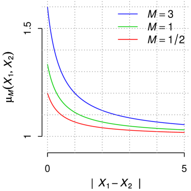
Figure 7: Dependence factor $\mu_{M}(X_{1},X_{2})=(M+1)^{2}\mathsf{E}\big{(}V(X_{1})V(X_{2})\big{)}$ w.r.t. $|X_{1}-X_{2}|$ for $M\in\{1/2,1,3\}$, where $\mathbf{V}$ is obtained by transforming a Gaussian process with squared exponential covariance function, with $\sigma_{Z}=1$ and $\lambda=1$.

Proposition 5

Let observations $\mathbf{Y}_{1}^{n}=(Y_{1,1},\ldots,Y_{n,1})$ and $\mathbf{Y}_{2}^{m}=(Y_{1,2},\ldots,Y_{m,2})$ at two sites $X_{1}$ and $X_{2}$, sampled from the data model (2) conditional to the process $\mathbf{p}\sim$$\mathsf{Dep}$-$\mathsf{GEM}$ $(M)$. The joint law of $Y_{1,1}$ and $Y_{1,2}$ is:

$$\mathsf{P}(Y_{1,1}=j,Y_{1,2}=k)=(M+1-\mu_{M})M^{|j-k|-1}(M^{2}-1+\mu_{M})^{(j\wedge k)-1}/(M+1)^{j+k},$$ (S.6)

for $k\neq j$ and

$$\mathsf{P}(Y_{1,1}=j,Y_{1,2}=j)=\mu_{M}(M^{2}-1+\mu_{M})^{j-1}/(M+1)^{2j},$$ (S.7)

where $\mu_{M}(X_{1},X_{2})=(M+1)^{2}\mathsf{E}\big{(}V(X_{1})V(X_{2})\big{)}$ and $j\wedge k=\min(j,k)$.

Equation (S.6) reduces to $M^{j+k-2}/(M+1)^{j+k}$ in the independent case (i.e. $V(X_{1})\mathchoice{\mathrel{\hbox to0.0pt{$\displaystyle\perp$\hss}\mkern 2.0mu{\displaystyle\perp}}}{\mathrel{\hbox to0.0pt{$\textstyle\perp$\hss}\mkern 2.0mu{\textstyle\perp}}}{\mathrel{\hbox to0.0pt{$\scriptstyle\perp$\hss}\mkern 2.0mu{\scriptstyle\perp}}}{\mathrel{\hbox to0.0pt{$\scriptscriptstyle\perp$\hss}\mkern 2.0mu{\scriptscriptstyle\perp}}}V(X_{2})$), which is indeed equal to $\mathsf{P}(Y_{1,1}=j)\mathsf{P}(Y_{1,2}=k)$. The probability that both first picks are equal is obtained by summing Equation (S.7) for all positive $j$:

$$\mathsf{P}(Y_{1,1}=Y_{1,2})=\frac{\mu_{M}}{2M+2-\mu_{M}}.$$ (S.8)

We can see that in the independent case, Equation (S.8) reduces to the probability that two draws at the same site $X_{1}$ belong to the same species, i.e. $\mathsf{P}(Y_{1,1}=Y_{2,1})={1}/{(2M+1)}$, obtained by summing all squares of $M^{j-1}/(M+1)^{j}$.

S.3.4 Size-biased permutations

In this section we derive some general results about size-biased permutations in a covariate-dependent model which are useful for the understanding of the $\mathsf{Dep}$-$\mathsf{GEM}$ model. Let $\mathbf{p}=(p_{1},p_{2},\ldots)$ be a probability. A size-biased permutation ($\mathsf{SBP}$) of $\mathbf{p}$ is a sequence $\tilde{\mathbf{p}}=(\tilde{p}_{1},\tilde{p}_{2},\ldots)$ obtained by reordering $\mathbf{p}$ by a permutation $\sigma$ with particular probabilities. Namely, the first index appears with a probability equal to its weight, $\mathsf{P}(\sigma_{1}=j)=p_{j}$ ; the subsequent indices appear with a probability proportional to their weight in the remaining indices, i.e. for $k$ distinct integers $j_{1},\ldots,j_{k}$,

$$\mathsf{P}(\sigma_{k}=j_{k}|\sigma_{1}=j_{1},\ldots,\sigma_{k-1}=j_{k-1})=\frac{p_{j_{k}}}{1-p_{j_{1}}-\ldots-p_{j_{k-1}}}.$$ (S.9)

We first extend Pitman’s following result (for example Equation (2.23) of Pitman,, 2006):

$$\mathsf{E}\Big{(}\sum f(p_{j})\Big{)}=\mathsf{E}\Big{(}\sum f(\tilde{p}_{j})\Big{)}=\mathsf{E}\bigg{(}\frac{f(\tilde{p}_{1})}{\tilde{p}_{1}}\bigg{)},$$ (S.10)

for any measurable function $f$.

Proposition 6

Let $\tilde{\mathbf{p}}$ is a size-biased permutation of $\mathbf{p}$. For any measurable function $f$ and any integer $k\geq 1$, we have

$$\mathsf{E}\bigg{(}\sum_{(*)}f(p_{i_{1}},\ldots,p_{i_{k}})\bigg{)}=\mathsf{E}\bigg{(}f(\tilde{p}_{1},\ldots,\tilde{p}_{k})\prod_{i=1}^{k}(1-\tilde{p}_{1}-\cdots-\tilde{p}_{i-1})/\tilde{p}_{i}\bigg{)},$$ (S.11)

where the sum $(*)$ runs over all distinct $i_{1},\ldots,i_{k}$, and with the convention that the product in the right-hand side of Equation (S.11) equals $1/\tilde{p}_{1}$ when $k=1$.

When it comes to averaging sums of transforms of $k$ weights $p_{i_{1}},\ldots,p_{i_{k}}$ over all distinct $i_{1},\ldots,i_{k}$, the proposition shows that all required information is encoded by the first $k$ picks $\tilde{p}_{1},\ldots,\tilde{p}_{k}$. As stated before, the special case for $k=1$ is a well known lemma. We also mention that the case $k=2$ was proved by Archer et al., (2014).

We can look for a further insight into the $\mathsf{Dep}$-$\mathsf{GEM}$ distribution by studying the exchangeable partition probability function ($\mathsf{EPPF}$) for the random variables $\mathbf{Y}_{1}^{n}=(Y_{1,1},\ldots,Y_{n,1})$ and $\mathbf{Y}_{2}^{m}=(Y_{1,2},\ldots,Y_{m,2})$ observed at covariates $X_{1}$ and $X_{2}$. See for instance Pitman, (1995, 2006) for a summary of the importance of partition probability functions. The observations partition $[n]=\{1,2,\ldots,n\}$ and $[m]=\{1,2,\ldots,m\}$ into $k+k_{1}+k_{2}$ clusters of distinct values where

• $k$ clusters are commonly observed, with respective frequencies $\textbf{n}=(n_{1},\ldots,n_{k})$ and $\textbf{m}=(m_{1},\ldots,m_{k})$,

• $k_{1}$ (resp. $k_{2}$) clusters are observed only at the site of covariate $X_{1}$ (resp. $X_{2}$), with frequencies $\tilde{\textbf{n}}=(\tilde{n}_{1},\ldots,\tilde{n}_{k_{1}})$ (resp. $\tilde{\textbf{m}}=(\tilde{m}_{1},\ldots,\tilde{m}_{k_{2}})$).

The $\mathsf{EPPF}$ can be expressed as follows

$$p(\textbf{n},\tilde{\textbf{n}},\textbf{m},\tilde{\textbf{m}}) =\mathsf{E}\bigg{(}\sum_{(*)}p_{i_{1}}^{n_{1}}(X_{1})p_{i_{1}}^{m_{1}}(X_{2})\ldots p_{i_{k}}^{n_{k}}(X_{1})p_{i_{k}}^{m_{k}}(X_{2})$$

$$\times p_{j_{1}}^{\tilde{n}_{1}}(X_{1})\ldots p_{j_{k_{1}}}^{\tilde{n}_{k_{1}}}(X_{1})\times p_{l_{1}}^{\tilde{m}_{1}}(X_{2})\ldots p_{l_{k_{2}}}^{\tilde{m}_{k_{2}}}(X_{2})\bigg{)}$$ (S.12)

where the sum $(*)$ runs over all $(k+k_{1}+k_{2})$-uples $(i_{1},\ldots,i_{k},j_{1},\ldots,j_{k_{1}},l_{1},\ldots,l_{k_{2}})$ with pairwise distinct elements.

In non covariate-dependent models, the $\mathsf{EPPF}$ can be derived as follows. The expression of Equation (S.3.4) reduces to a simpler sum $p(\textbf{n})$ which equals the conditional expectation of the first few elements of a size-biased permutation $\tilde{\mathbf{p}}$ given $\mathbf{p}$, and one obtains, by application of Proposition 6 where $f(p_{1},\ldots,p_{k})=p_{1}^{n_{1}}\ldots p_{k}^{n_{k}}$:

$$p(\textbf{n})=\mathsf{E}\bigg{[}\prod_{i=1}^{k}\tilde{p}_{i}^{n_{i}-1}\prod_{i=1}^{k-1}\Big{(}1-\sum_{j=1}^{i}\tilde{p}_{j}\Big{)}\bigg{]}.$$

The invariance under size-biased permutation ($\mathsf{ISBP}$) property that characterizes the $\mathsf{GEM}$ distribution (cf. Pitman,, 1996) can then be used to replace the first few elements of the size-biased permutation $\tilde{\mathbf{p}}$ by the first few elements of $\mathbf{p}$:

$$p(\textbf{n})=\mathsf{E}\bigg{[}\prod_{i=1}^{k}p_{i}^{n_{i}-1}\prod_{i=1}^{k-1}\Big{(}1-\sum_{j=1}^{i}p_{j}\Big{)}\bigg{]}.$$

The final steps are to use the stick-breaking representation of $\mathbf{p}$ with independent Beta random variables $\mathbf{V}$, and derive the $\mathsf{EPPF}$ by computing the moments of Beta random variables (see Equation (S.13))

$$p(\textbf{n})=\frac{M^{k}}{M_{(n)}}\prod_{j=1}^{k}\left(n_{j}-1\right)!$$

Here, the hindrance to further computation of a closed-form expression for $p(\textbf{n},\tilde{\textbf{n}},\textbf{m},\tilde{\textbf{m}})$ in (S.3.4) is, to the best of our knowledge, twofold: (i) the sum in Equation (S.3.4) does not reduce to any conditional expectation of the first few elements of a size-biased permutation of $\mathbf{p}$, and (ii) the invariance under size-biased permutation property is not straightforward to generalize to covariate-dependent distributions, hence equality in distribution between $(\tilde{p}_{1}(X_{1}),\tilde{p}_{1}(X_{2}))$ and $(p_{1}(X_{1}),p_{1}(X_{2}))$ is not a known property (whereas it is marginally true).

Notwithstanding this, $\mathsf{EPPF}$ have been obtained in the covariate-dependent literature, though not for stick-breaking constructions, but when the dependent process is defined by normalizing random probability measures, such as completely random measures. See for instance Lijoi et al., 2013a ; Kolossiatis et al., (2013); Griffin et al., (2013). See also Müller et al., (2011) for an approach based on product partition models.

S.4 Proofs

Proof of Proposition 2

The process $\mathbf{V}$ constructed in the main paper is marginally $\mathsf{Beta}(1,M)$, hence by the stick-breaking construction, the process $\mathbf{p}\sim$$\mathsf{Dep}$-$\mathsf{GEM}$ $(M)$ has marginally the $\mathsf{GEM}(M)$ distribution. Let $\mathbf{\mathcal{Z}}\sim\mathsf{GP}$ as defined in the paper, and suppose for simplicity of notations that it is defined on $\mathcal{X}=\mathbb{R}$. Gaussian processes have continuous paths, which in turn holds for $\mathcal{V}=F_{M}^{-1}\circ\Phi_{\sigma_{\mathbf{\mathcal{Z}}}}(\mathbf{\mathcal{Z}})$ since the transformation $F_{M}^{-1}\circ\Phi_{\sigma_{\mathbf{\mathcal{Z}}}}$ is the composition of continuous functions. Denote by $\mathcal{V}_{1},\mathcal{V}_{2},\ldots$ independent processes of this type, and define $\mathbf{p}=(\mathbf{p}_{1},\mathbf{p}_{2},\ldots)$ by stick-breaking, $\mathbf{p}_{j}=\Psi_{j}(\mathcal{V}_{1},\ldots,\mathcal{V}_{j})=\mathcal{V}_{j}\prod_{l<j}(1-\mathcal{V}_{l})$. Then for any $j$, $\Psi_{j}$ is a continuous function from $(0,1)^{j}$ to $(0,1)$, so $\mathbf{p}_{j}$ has continuous paths. This means that $\mathbf{p}=(\mathbf{p}_{1},\mathbf{p}_{2},\ldots)$ has continuous paths in the sup norm topology.

The expressions for the moments of $p_{j}(X)$ are derived by using the following moments of a random variable $V\sim\mathsf{Beta}(\alpha,\beta)$, for any $j,k\geq 0$:

$$\mathsf{E}(V^{k})=\frac{\alpha_{(k)}}{(\alpha+\beta)_{(k)}}\,\text{ and }\,\mathsf{E}\big{(}V^{k}(1-V)^{j}\big{)}=\frac{\alpha_{(k)}\beta_{(j)}}{(\alpha+\beta)_{(k+j)}}.$$ (S.13)

We omit the dependence in $X$ in order to simplify the notation. Note that for $V\sim\mathsf{Beta}(1,M)$, one has $\bar{V}=1-V\sim\mathsf{Beta}(M,1)$. For any $n\geq 0$, $\mathsf{E}(p_{j}^{n})$ follows from

$$\mathsf{E}(p_{j}^{n})=\mathsf{E}\big{(}V_{j}^{n}\prod_{l<j}(1-V_{l})^{n}\big{)}=\frac{1_{(n)}}{(M+1)_{(n)}}\Big{(}\frac{1_{(n)}}{(M+1)_{(n)}}\Big{)}^{j-1}.$$ (S.14)

The formula for $\mathsf{Var}(p_{j})$ is obtained as a consequence of (S.14), while $\mathsf{Cov}(p_{j},p_{k})$, $k\neq j$, requires the computation of $\mathsf{E}(p_{j}p_{k})$ as follows (suppose without loss of generality that $j>k$)

$$\mathsf{E}(V_{j}) \cdot\prod_{j>l>k}\mathsf{E}(\bar{V}_{l})\cdot\mathsf{E}(V_{k}\bar{V}_{k})\cdot\prod_{k>l}\mathsf{E}(\bar{V}_{l}^{2})$$

$$=\frac{1}{M+1}\Big{(}\frac{M}{M+1}\Big{)}^{j-k-1}\Big{(}\frac{1}{M+1}-\frac{2}{(M+1)(M+2)}\Big{)}\Big{(}\frac{M}{M+2}\Big{)}^{k-1}$$

$$=\frac{M^{j-1}}{(M+1)^{j-k+1}(M+2)^{k}}.$$

$\square$

Proof of Proposition 3

Let $\Psi:(0,1)^{\mathbb{N}}\rightarrow\mathcal{S}$ be the stick-breaking transform. It has a reciprocal defined on $\mathcal{S}$ whose coordinates are given by

$$V_{1}=p_{1},\quad V_{j}=p_{j}(1-\sum_{l=1}^{j-1}p_{l})^{-1},\quad j\geq 2,$$

which are in $(0,1)$ by construction because for all $j$, $0<p_{j}<1$.

Let $\epsilon>0$ and $p^{*}\in\mathcal{S}$. Denote by $V^{*}$ the reciprocal of $p^{*}$. Let $M=\min\{m:\lVert p_{1:m}^{*}\rVert_{1}>1-\epsilon/3\}$. Denote by $\Psi_{M}$ the restriction of $\Psi$ to its first $M$ coordinates. We have by construction $\Psi_{M}(V_{1:M}^{*})=p_{1:M}^{*}$. Since $\Psi_{M}$ is continuous and $\lVert p_{1:M}^{*}\rVert_{1}>1-\epsilon/3$, there exist two neighborhoods of $V_{1:M}^{*}$ in $(0,1)^{M}$, denoted by $A_{\epsilon}$ and $B_{\epsilon}$, such that

$$\forall V_{1:M}\in A_{\epsilon},\quad\lVert p_{1:M}\rVert_{1}>1-\epsilon/3\text{ for }p_{1:M}=\Psi_{M}(V_{1:M})$$

and

$$\forall V_{1:M}\in B_{\epsilon},\quad\lVert p_{1:M}^{*}-p_{1:M}\rVert_{1}\leq\epsilon/3\text{ for }p_{1:M}=\Psi_{M}(V_{1:M})$$

The intersection of $A_{\epsilon}$ and $B_{\epsilon}$ is an open set of $(0,1)^{M}$ which has no trivial coordinate because it contains $V_{1:M}^{*}$. Denote by $D=(A_{\epsilon}\cap B_{\epsilon})\times(0,1)^{\mathbb{N}}$. Then for any $V\in D$, the image $p=\Psi(V)$ satisfies

$$\lVert p-p^{*}\rVert_{1}\leq\lVert p_{1:M}-p_{1:M}^{*}\rVert_{1}+1-\lVert p_{1:M}^{*}\rVert_{1}+1-\lVert p_{1:M}\rVert_{1}\leq\epsilon$$

In addition, $D$ has positive prior mass, which proves the proposition. $\square$

Proof of Proposition 4

The proof follows the same line as that of Proposition 3. For the sake of simplicity and without loss of generality we assume that $\int_{\mathcal{X}}dx=1$. Let $\mathbf{p}^{\star}(.)=\psi(\mathbf{v}^{\star})$ with $\mathbf{v}^{\star}=(v_{j}^{\star},j\geq 1)$ and $v_{j}^{\star}\in\mathbf{H}$ for all $j\geq 1$. Then since $F_{M}(x)=\sum_{j=1}^{M}p_{j}^{\star}(x)$ is an increasing sequence (in $M$) to the constant function $1$, $\int_{\mathcal{X}}F_{M}(x)dx\uparrow 1$ and there exists $M^{\epsilon}$ such that

$$\int_{\mathcal{X}}F_{M^{\epsilon}}(x)dx\geq 1-\epsilon/3.$$

The operator $\mathbf{\psi}_{M}:\mathbb{H}^{M}\rightarrow\mathcal{C}(\mathcal{X})^{M}$ defined by $\mathbf{\psi}_{M}(V_{j}(.),j\leq M)=(V_{j}\prod_{i<j}(1-V_{i})(.),j\leq M)$ is continuous for the $L_{1}$ norm on $\mathcal{X}$ for all $M$. Hence there exists an $L_{1}$ open neighbourhood of $(v_{j}^{\star},j\leq M^{\star})$, say $V_{\epsilon}$ such that if $(v_{j},j\leq M^{\star})\in V_{\epsilon}$

$$\sum_{j=1}^{M^{\star}}\|p_{j}-p_{j}^{\star}\|_{1}\leq\epsilon/3,\quad(p_{j},j\leq M^{\star})=\mathbf{\psi}_{M^{\star}}(v_{j},j\leq M^{\star})$$

the rest of the proof is the same as in the case of Proposition 3. $\square$

Proof of Proposition 5

By conditional independence

$$\mathsf{P}(Y_{1,1}=j,Y_{1,2}=k) =\mathsf{E}\big{(}\mathsf{P}(Y_{1,1}=j,Y_{1,2}=k\,|\,\mathbf{p}(X_{1}),\mathbf{p}(X_{2}))\big{)}$$

$$=\mathsf{E}(p_{j}(X_{1})p_{k}(X_{2})).$$

Suppose that $j>k$, (the case $j<k$ is symmetric) then the last quantity can be decomposed into the following product of four groups of terms

$$\begin{array}[]{@{}r@{}@{}c@{}@{}c@{}@{}c@{}@{}c@{}@{}c@{}@{}c@{}@{}c@{}}&\mathsf{E}(V_{j}(X_{1}))&\,\cdot&\prod_{k<l<j}\mathsf{E}(\bar{V}_{l}(X_{1}))&\,\cdot&\mathsf{E}(\bar{V}_{k}(X_{1})V_{k}(X_{2}))&\,\cdot&\prod_{l<k}\mathsf{E}(\bar{V}_{l}(X_{1})\bar{V}_{l}(X_{2}))\\ &=\frac{1}{M+1}&\,\cdot&\Big{(}\frac{M}{M+1}\Big{)}^{j-k-1}&\,\cdot&\Big{(}\frac{1}{M+1}-\frac{\mu_{M}}{(M+1)^{2}}\Big{)}&\,\cdot&\Big{(}1-\frac{2}{M+1}+\frac{\mu_{M}}{(M+1)^{2}}\Big{)}^{k-1}\end{array}$$

which sums up to the desired quantity. The case $k=j$ is treated in a similar fashion. $\square$

Proof of Proposition 6

By definition of the size-biased permutation, $\mathsf{P}(\tilde{p}_{1}=p_{i}\,|\,\mathbf{p})=p_{i}$, $\mathsf{P}(\tilde{p}_{2}=p_{i_{2}}\,|\,\tilde{p}_{1}=p_{i_{1}},\mathbf{p})=\frac{p_{i_{2}}}{1-p_{i_{1}}}$, and

$$\mathsf{P}\big{[}(\tilde{p}_{1},\ldots,\tilde{p}_{k})=(p_{i_{1}},\ldots,p_{i_{k}})\,|\,\mathbf{p}\big{]}=\prod_{l=1}^{k}\frac{p_{i_{l}}}{1-p_{i_{1}}-\cdots-p_{i_{l-1}}}.$$ (S.15)

Hence the right-hand side term in Proposition 6 can be computed by double expectation and conditioning on $\mathbf{p}$

$$\mathsf{E}\big{[}(\mathsf{E}\big{(}f(\tilde{p}_{1},\ldots,\tilde{p}_{k})\prod_{i=1}^{k}(1-\tilde{p}_{1}-\cdots-\tilde{p}_{i-1})/\tilde{p}_{i}\,|\,\mathbf{p}\big{)}\big{]},$$

and a simplification arises with the probability of (S.15) when enumerating over all distinct indices $i_{1},\ldots,i_{k}$. $\square$

Proof of Proposition 1 of the main document

Let $\bar{H}(X)=1-H_{\mathsf{\scriptstyle Simp}}(X)=\sum_{j}p_{j}^{2}(X)$. Then $\mathsf{Cov}(H_{\mathsf{\scriptstyle Simp}}(X_{1}),H_{\mathsf{\scriptstyle Simp}}(X_{2}))=\mathsf{Cov}(\bar{H}(X_{1}),\bar{H}(X_{2}))$. First note that $\mathsf{E}(\bar{H}(X)=\mathsf{E}(p_{1}(X))=\mathsf{E}(V_{1}(X))=1/(M+1)$ by virtue of Equation (S.10). Then $\mathsf{E}(\bar{H}(X_{1})\bar{H}(X_{2}))$ is obtained by summing the following terms:

$$\text{for all }\,j\geq 1,\,\mathsf{E}(p_{j}(X_{1})p_{j}(X_{2}))=\nu_{2,2}\omega_{2,2}^{j-1},$$

$$\text{for all }\,j\neq k\geq 1,\,\mathsf{E}(p_{j}(X_{1})p_{k}(X_{2}))=\nu_{2,0}\omega_{2,0}^{|j-k|-1}\gamma_{2,2}\omega_{2,2}^{(j\wedge k)-1},$$

where the same kind of development as in the proof of Proposition 5 is employed. For the variance of the Simpson index, one needs, by omitting the covariate $X$ in the notation

$$\mathsf{E}\Big{(}\big{(}\sum_{j}p_{j}^{2}\big{)}^{2}\Big{)} =\mathsf{E}\Big{(}\sum_{i,j}p_{i}^{2}p_{j}^{2}\Big{)}=\mathsf{E}\Big{(}\sum_{i\neq j}p_{i}^{2}p_{j}^{2}\Big{)}+\mathsf{E}\Big{(}\sum_{i}p_{j}^{4}\Big{)}$$

$$=\mathsf{E}(p_{1}(1-p_{1})p_{2})+\mathsf{E}(p_{1}^{3})=\mathsf{E}(V_{1}(1-V_{1})^{2})\mathsf{E}(V_{2})+\mathsf{E}(V_{1}^{3})$$

$$=(M+6)/(M+1)_{(3)},$$

by Proposition 6 and the moments (S.13). $\square$

References

- Aitchison, (1982) Aitchison, J. (1982). The statistical analysis of compositional data. Journal of the Royal Statistical Society. Series B (Methodological), pages 139–177.
- Arbel, (2013) Arbel, J. (2013). Contributions to Bayesian nonparametric statistics. PhD thesis, Université Paris-Dauphine.
- (3) Arbel, J., Favaro, S., Nipoti, B., and Teh, Y. W. (2015a). Bayesian nonparametric inference for discovery probabilities: credible intervals and large sample asymptotics. Submitted. arxiv:1506.04915.
- (4) Arbel, J., Mengersen, K., Raymond, B., Winsley, T., and King, C. (2015b). Application of a Bayesian nonparametric model to derive toxicity estimates based on the response of Antarctic microbial communities to fuel contaminated soil. Ecology and Evolution.
- (5) Arbel, J., Mengersen, K., and Rousseau, J. (2015c). Supplementary Material for the paper “Bayesian nonparametric dependent model for partially replicated data: the influence of fuel spills on species diversity”. arXiv:1402.3093.
- Archer et al., (2014) Archer, E., Park, I. M., and Pillow, J. W. (2014). Bayesian entropy estimation for countable discrete distributions. The Journal of Machine Learning Research, 15(1):2833–2868.
- Barrientos et al., (2012) Barrientos, A. F., Jara, A., and Quintana, F. A. (2012). On the support of MacEachern’s dependent Dirichlet processes and extensions. Bayesian Analysis, 7(2):277–310.
- Barrientos et al., (2015) Barrientos, A. F., Jara, A., and Quintana, F. A. (2015). Bayesian density estimation for compositional data using random Bernstein polynomials. Journal of Statistical Planning and Inference.
- Bissiri et al., (2014) Bissiri, P. G., Ongaro, A., et al. (2014). On the topological support of species sampling priors. Electronic Journal of Statistics, 8:861–882.
- Bohlin et al., (2009) Bohlin, J., Skjerve, E., and Ussery, D. (2009). Analysis of genomic signatures in prokaryotes using multinomial regression and hierarchical clustering. BMC Genomics, 10(1):487.
- Borges and Roditi, (1998) Borges, E. P. and Roditi, I. (1998). A family of nonextensive entropies. Physics Letters A, 246(5):399–402.
- Caron et al., (2007) Caron, F., Davy, M., and Doucet, A. (2007). Generalized polya urn for time-varying dirichlet process mixtures.
- Cerquetti, (2014) Cerquetti, A. (2014). Bayesian nonparametric estimation of Patil-Taillie-Tsallis diversity under Gnedin-Pitman priors. arXiv preprint arXiv:1404.3441.
- Chung and Dunson, (2009) Chung, Y. and Dunson, D. (2009). The local Dirichlet process. Annals of the Institute of Statistical Mathematics, pages 1–22.
- Colwell et al., (2012) Colwell, R. K., Chao, A., Gotelli, N. J., Lin, S.-Y., Mao, C. X., Chazdon, R. L., and Longino, J. T. (2012). Models and estimators linking individual-based and sample-based rarefaction, extrapolation and comparison of assemblages. Journal of Plant Ecology, 5:3–21.
- De’ath, (2012) De’ath, G. (2012). The multinomial diversity model: linking Shannon diversity to multiple predictors. Ecology, 93(10):2286–2296.
- Donnelly and Grimmett, (1993) Donnelly, P. and Grimmett, G. (1993). On the asymptotic distribution of large prime factors. Journal of the London Mathematical Society, 2(3):395–404.
- Dorazio et al., (2008) Dorazio, R. M., Mukherjee, B., Zhang, L., Ghosh, M., Jelks, H. L., and Jordan, F. (2008). Modeling unobserved sources of heterogeneity in animal abundance using a Dirichlet process prior. Biometrics, 64(2):635–644.
- Dunson and Park, (2008) Dunson, D. and Park, J. (2008). Kernel stick-breaking processes. Biometrika, 95(2):307.
- Dunson et al., (2007) Dunson, D., Pillai, N., and Park, J. (2007). Bayesian density regression. Journal of the Royal Statistical Society: Series B (Statistical Methodology), 69(2):163–183.
- Dunson and Xing, (2009) Dunson, D. B. and Xing, C. (2009). Nonparametric Bayes modeling of multivariate categorical data. Journal of the American Statistical Association, 104(487).
- Dunstan et al., (2011) Dunstan, P. K., Foster, S. D., and Darnell, R. (2011). Model based grouping of species across environmental gradients. Ecological Modelling, 222(4):955–963.
- Ellis et al., (2011) Ellis, N., Smith, S. J., and Pitcher, C. R. (2011). Gradient forests: calculating importance gradients on physical predictors. Ecology, 93(1):156–168.
- Favaro et al., (2012) Favaro, S., Lijoi, A., and Prünster, I. (2012). A new estimator of the discovery probability. Biometrics, 68(4):1188–1196.
- Favaro et al., (2015) Favaro, S., Nipoti, B., and Teh, Y. W. (2015). Rediscovery of Good–Turing estimators via Bayesian nonparametrics. Biometrics, in press. arXiv preprint arXiv:1401.0303.
- Ferguson, (1973) Ferguson, T. (1973). A Bayesian analysis of some nonparametric problems. The Annals of Statistics, 1(2):209–230.
- Ferrier and Guisan, (2006) Ferrier, S. and Guisan, A. (2006). Spatial modelling of biodiversity at the community level. Journal of Applied Ecology, 43(3):393–404.
- Ferrier et al., (2007) Ferrier, S., Manion, G., Elith, J., and Richardson, K. (2007). Using generalized dissimilarity modelling to analyse and predict patterns of beta diversity in regional biodiversity assessment. Diversity and Distributions, 13:252–264.
- Fordyce et al., (2011) Fordyce, J. A., Gompert, Z., Forister, M. L., and Nice, C. C. (2011). A hierarchical Bayesian approach to ecological count data: a flexible tool for ecologists. PLoS ONE, 6(11):e26785.
- Foster and Dunstan, (2010) Foster, S. D. and Dunstan, P. K. (2010). The analysis of biodiversity using rank abundance distributions. Biometrics, 66(1):186–195.
- Gelfand, (1996) Gelfand, A. E. (1996). Model determination using sampling-based methods. Markov chain Monte Carlo in practice, pages 145–161.
- Gibbs, (1997) Gibbs, M. N. (1997). Bayesian Gaussian processes for regression and classification. PhD thesis, Citeseer.
- Gill and Joanes, (1979) Gill, C. A. and Joanes, D. N. (1979). Bayesian estimation of Shannon’s index of diversity. Biometrika, 66(1):81–85.
- Good, (1953) Good, I. J. (1953). The population frequencies of species and the estimation of population parameters. Biometrika, 40(3-4):237–264.
- Griffin and Steel, (2006) Griffin, J. and Steel, M. (2006). Order-based dependent Dirichlet processes. Journal of the American statistical Association, 101(473):179–194.
- Griffin et al., (2013) Griffin, J. E., Kolossiatis, M., and Steel, M. F. (2013). Comparing distributions by using dependent normalized random-measure mixtures. Journal of the Royal Statistical Society: Series B (Statistical Methodology), 75(3):499–529.
- Griffin and Steel, (2011) Griffin, J. E. and Steel, M. F. (2011). Stick-breaking autoregressive processes. Journal of econometrics, 162(2):383–396.
- Havrda and Charvát, (1967) Havrda, J. and Charvát, F. (1967). Quantification method of classification processes. Concept of structural -entropy. Kybernetika, 3(1):30–35.
- Hill, (1973) Hill, M. O. (1973). Diversity and evenness: a unifying notation and its consequences. Ecology, 54(2):427–432.
- Holmes et al., (2012) Holmes, I., Harris, K., and Quince, C. (2012). Dirichlet Multinomial Mixtures: Generative Models for Microbial Metagenomics. PloS one, 7(2):e30126.
- Ishwaran and James, (2001) Ishwaran, H. and James, L. (2001). Gibbs sampling methods for stick-breaking priors. Journal of the American Statistical Association, 96(453):161–173.
- Johnson et al., (2013) Johnson, D. S., Ream, R. R., Towell, R. G., Williams, M. T., and Guerrero, J. D. L. (2013). Bayesian clustering of animal abundance trends for inference and dimension reduction. Journal of Agricultural, Biological, and Environmental Statistics, 18(3):299–313.
- Kaniadakis et al., (2005) Kaniadakis, G., Lissia, M., and Scarfone, A. (2005). Two-parameter deformations of logarithm, exponential, and entropy: a consistent framework for generalized statistical mechanics. Physical Review E, 71(4):046128.
- Kolossiatis et al., (2013) Kolossiatis, M., Griffin, J. E., and Steel, M. F. (2013). On Bayesian nonparametric modelling of two correlated distributions. Statistics and Computing, 23(1):1–15.
- Lijoi et al., (2007) Lijoi, A., Mena, R. H., and Prünster, I. (2007). Bayesian nonparametric estimation of the probability of discovering new species. Biometrika, 94(4):769–786.
- (46) Lijoi, A., Nipoti, B., and Prünster, I. (2013a). Bayesian inference with dependent normalized completely random measures. Bernoulli, 20(3):1260–1291.
- (47) Lijoi, A., Nipoti, B., and Prünster, I. (2013b). Dependent mixture models: clustering and borrowing information. Computational Statistics and Data Analysis, 71:417–433.
- MacEachern, (1999) MacEachern, S. (1999). Dependent nonparametric processes. ASA Proceedings of the Section on Bayesian Statistical Science, pages 50–55.
- MacEachern, (2000) MacEachern, S. N. (2000). Dependent Dirichlet processes. Technical report, Department of Statistics, The Ohio State University.
- Müller et al., (2011) Müller, P., Quintana, F. A., and Rosner, G. L. (2011). A product partition model with regression on covariates. Journal of Computational and Graphical Statistics, 20(1).
- Newman, (2012) Newman, M. C. (2012). Quantitative ecotoxicology. CRC Press.
- Pati et al., (2013) Pati, D., Dunson, D. B., and Tokdar, S. T. (2013). Posterior consistency in conditional distribution estimation. Journal of multivariate analysis, 116:456–472.
- Patil and Taillie, (1982) Patil, G. and Taillie, C. (1982). Diversity as a concept and its measurement. Journal of the American statistical Association, 77(379):548–561.
- Pitman, (1995) Pitman, J. (1995). Exchangeable and partially exchangeable random partitions. Probability Theory and Related Fields, 102(2):145–158.
- Pitman, (1996) Pitman, J. (1996). Random discrete distributions invariant under size-biased permutation. Advances in Applied Probability, pages 525–539.
- Pitman, (2006) Pitman, J. (2006). Combinatorial stochastic processes, volume 1875. Springer-Verlag.
- Rasmussen and Williams, (2006) Rasmussen, C. E. and Williams, C. K. I. (2006). Gaussian Processes for Machine Learning. MIT Press.
- Rodriguez and Dunson, (2011) Rodriguez, A. and Dunson, D. B. (2011). Nonparametric Bayesian models through probit stick-breaking processes. Bayesian Analysis, 6(1):145–177.
- Rodriguez et al., (2010) Rodriguez, A., Dunson, D. B., and Gelfand, A. E. (2010). Latent stick-breaking processes. Journal of the American Statistical Association, 105(490).
- Royle and Dorazio, (2006) Royle, J. A. and Dorazio, R. M. (2006). Hierarchical models of animal abundance and occurrence. Journal of Agricultural, Biological, and Environmental Statistics, 11(3):249–263.
- Royle and Dorazio, (2008) Royle, J. A. and Dorazio, R. M. (2008). Hierarchical modeling and inference in ecology: the analysis of data from populations, metapopulations and communities. Academic Press.
- Rue et al., (2009) Rue, H., Martino, S., and Chopin, N. (2009). Approximate Bayesian inference for latent Gaussian models by using integrated nested Laplace approximations. Journal of the Royal Statistical Society: Series B (Statistical Methodology), 71(2):319–392.
- Schloss et al., (2009) Schloss, P. D., Westcott, S. L., Ryabin, T., Hall, J. R., Hartmann, M., Hollister, E. B., Lesniewski, R. A., Oakley, B. B., Parks, D. H., Robinson, C. J., Sahl, J. W., Stres, B., Thallinger, G. G., Van Horn, D. J., and Weber, C. F. (2009). Introducing mothur: open-source, platform-independent, community-supported software for describing and comparing microbial communities. Applied and Environmental Microbiology, 75(23):7537–41.
- Siciliano et al., (2014) Siciliano, S. D., Palmer, A. S., Winsley, T., Lamb, E., Bissett, A., Brown, M. V., van Dorst, J., Ji, M., Ferrari, B. C., Grogan, P., Chu, H., and Snape, I. (2014). Fertility controls richness but pH controls composition in polar microbial communities. Soil Biology and Biochemistry, Submitted.
- Snape et al., (2015) Snape, I., Siciliano, S. D., Winsley, T., van Dorst, J., Mukan, J., Palmer, A. S., and Lagerewskij, G. (2015). Operational Taxonomic Unit (OTU) Microbial Ecotoxicology data from Macquarie Island and Casey Station: TPH, Chemistry and OTU Abundance data. Australian Antarctic Data Centre.
- van der Vaart and van Zanten, (2009) van der Vaart, A. W. and van Zanten, J. (2009). Adaptive Bayesian estimation using a Gaussian random field with inverse Gamma bandwidth. The Annals of Statistics, 37(5B):2655–2675.
- Wang et al., (2012) Wang, Y., Naumann, U., Wright, S. T., and Warton, D. I. (2012). mvabund– an R package for model-based analysis of multivariate abundance data. Methods in Ecology and Evolution, 3(3):471–474.
Supplementary Material for