Adaptation in tunably rugged fitness landscapes:
The Rough Mount Fuji Model

Abstract

Much of the current theory of adaptation is based on Gillespie’s mutational landscape model (MLM), which assumes that the fitness values of genotypes linked by single mutational steps are independent random variables. On the other hand, a growing body of empirical evidence shows that real fitness landscapes, while possessing a considerable amount of ruggedness, are smoother than predicted by the MLM. In the present article we propose and analyse a simple fitness landscape model with tunable ruggedness based on the Rough Mount Fuji (RMF) model originally introduced by Aita et al. [Biopolymers 54:64-79 (2000)] in the context of protein evolution. We provide a comprehensive collection of results pertaining to the topographical structure of RMF landscapes, including explicit formulae for the expected number of local fitness maxima, the location of the global peak, and the fitness correlation function. The statistics of single and multiple adaptive steps on the RMF landscape are explored mainly through simulations, and the results are compared to the known behavior in the MLM model. Finally, we show that the RMF model can explain the large number of second-step mutations observed on a highly-fit first step backgound in a recent evolution experiment with a microvirid bacteriophage [Miller et al., Genetics 187:185-202 (2011)].

The genetic adaptation of an asexual population to a novel environment is governed by the number and fitness effects of available beneficial mutations, their epistatic interactions, and the rate at which they are supplied [Sniegowski and Gerrish (2010]. Despite the inherent complexity of this process, recent theoretical work has identified several robust statistical patterns of adaptive evolution [Orr (2005a, Orr (2005b]. Most of these predictions were derived in the framework of Gillespie’s mutational landscape model (MLM), which is based on three key assumptions [Gillespie (1983, Gillespie (1984, Gillespie (1991, Orr (2002b]. First, selection is strong enough to prevent the fixation of deleterious mutations and mutation is sufficiently weak such that mutations emerge and fix one at a time (the strong selection/weak mutation or SSWM regime). Second, wildtype fitness is high, which allows one to describe the statistics of beneficial mutations using extreme value theory (EVT). Third, the fitness values of new mutants are uncorrelated with the fitness of the ancestor from which they arise. This last assumption implies that the fitness landscape underlying the adaptive process is maximally rugged with many local maxima and minima [Kauffman and Levin (1987, Kauffman (1993, Jain and Krug (2007], a limiting situation that is often referred to as the House of Cards (HoC) landscape [Kingman (1978]. Thus, the MLM is concerned with a population evolving in a HoC landscape under SSWM dynamics, starting from an initial state of high fitness.

The validity of the SSWM assumption depends primarily on the population size $N$. Denoting the mutation rate by $u$ and the typical selection strength by $s$, the criterion for the SSWM regime reads $Nu\ll 1\ll Ns$, which can always be satisfied by a suitable choice of $N$ provided $u\ll s$, as is usually the case. On the other hand, whether or not the other two assumptions underlying the MLM are realistic is an empirical question that has been addressed in a number of experimental studies of microbial evolution. Investigations aimed at determining the distribution of effect sizes of benefical mutations have generally found support for the EVT hypothesis [Orr (2003, Joyce et al. (2008, Orr (2010], and examples for all three EVT universality classes have been reported in the literature [Rokyta et al. (2005, Kassen and Bataillon (2006, Rokyta et al. (2008, MacLean and Buckling (2009, Schenk et al. (2012, Foll et al. (2014, Bank et al. (2014]. At the same time, however, it has become increasingly clear that the extreme assumption of uncorrelated fitness values between genotypes connected by single mutational steps cannot be upheld in the face of empirical evidence.

Indications for the presence of correlations in real fitness landscapes derive from two types of experimental studies. In one approach, a subset of the fitness landscape is explicitly generated by constructing genotypes containing all combinations of a small group of mutations chosen for either individual or collective effects, and measuring their fitness or some proxy thereof [Weinreich et al. (2006, Lozovsky et al. (2009, Franke et al. (2011, Schenk et al. (2013, Szendro, Schenk et al. (2013, Weinreich et al. (2013, de Visser and Krug (2014]. Although the topographic properties of the resulting landscapes vary over a broad range, in most cases they display a degree of ruggedness that is intermediate between a smooth, additive landscape and the maximally rugged landscape assumed by the MLM [Szendro, Schenk et al. (2013, de Visser and Krug (2014]. In a second approach, properties of the underlying landscape are inferred from the observed dynamics of adaptation as manifested, for example, in the trajectories of fitness increase [Kryazhimskiy et al. (2009] or the number of substitutions in an adaptive walk [Gifford et al. (2011, Schoustra et al. (2012]. Of particular interest in the present context is the recent study of ?) on the microvirid bacteriophage ID11, where the MLM was tested by comparing the distribution of beneficial mutations from the wildtype to the corresponding distribution after one step of adaptation. According to the MLM, the two distributions should be identical up to a rescaling, but this hypothesis was clearly refuted by the experiment.

The observation that most empirical fitness landscapes display an intermediate degree of ruggedness implies that there is a need for simple, mathematically tractable landscape models in which the ruggedness can be tuned. A frequently used model with tunable ruggedness is Kauffman’s “NK”-landscape where each of $L$ binary loci interacts randomly with $K$ other loci, and the interaction degree $K$ serves to interpolate between the additive limit $K=0$ and the HoC limit $K=L-1$ [Kauffman and Weinberger (1989, Kauffman (1993, Ohta (1997, Welch and Waxman (2005, Aita (2008, Østman et al. (2012, Franke and Krug (2012]. In the original definition of the NK-model the letter ‘N’ stands for the sequence length which we denote by $L$ in the present paper. While this model has been shown to be capable of describing various features of empirical fitness landscapes [Hayashi et al. (2006, Rowe et al. (2010, Franke et al. (2011], its mathematical complexity is such that even rather elementary properties – for example, the mean number of local fitness maxima [Evans and Steinsaltz (2002, Durrett and Limic (2003, Limic and Pemantle (2004] – are difficult to derive in closed form (but see ?), ?) and ?) for a variant of the NK-model that is simpler to analyze).

In the present article we therefore propose the Rough Mount Fuji (RMF) model as an alternative description of fitness landscapes with tunable ruggedness. The model is a simplified version of the RMF fitness landscape originally introduced by ?) in the context of protein evolution. In essence, the RMF model superimposes an additive fitness landscape and an uncorrelated random HoC landscape, and the ruggedness is tuned by changing the ratio of the additive selection coefficient to the standard deviation of the random fitness component [Aita and Husimi (2000, Franke et al. (2011, Szendro, Schenk et al. (2013]. Below we derive simple, explicit formulae for various quantitative measures of the RMF topography such as the number and location of local fitness maxima and fitness correlations. Moreover, assuming SSWM conditions, we show how the adaptation of a population on the RMF landscape can be efficiently simulated for realistic numbers of loci by locally generating the mutational neighborhood of the current genotype along the adaptive trajectory. Finally, as an example for the application of the RMF model to empirical fitness landscapes, we estimate the parameters of the fitness landscape of the microvirid bacteriophage ID11 studied by ?) by matching the number of secondary beneficial mutations available after one adaptive step (the number of exceedances) predicted by the model to the experimentally observed value.

Model

Definition.

Following a common practice in the description of empirical fitness landscapes, we represent genotypes by binary sequences $\sigma=(\sigma_{1},\sigma_{2},....,\sigma_{L})$ of fixed length $L$, composed of elements taken from the set $\{0,1\}$ with $\sigma_{i}=1$ ($\sigma_{i}=0$) if a mutation is present (absent) at the $i$’th locus. The set all binary sequences of length $L$ is known as the Hamming space. It is endowed with a natural distance measure, the Hamming distance defined as

$$D(\sigma,\sigma^{\prime})=\sum_{j=1}^{L}(\sigma_{j}-\sigma^{\prime}_{j})^{2}$$ (1)

which simply counts number the loci at which $\sigma$ and $\sigma^{\prime}$ differ. It is convenient to introduce the antipodal (or reversal) sequence $\overline{\sigma}$ of $\sigma$ through $\overline{\sigma}_{i}=1-\sigma_{i}$. A sequence and its antipode are maximally distant from each other, $D(\sigma,\overline{\sigma})=L$.

To introduce the Rough Mount Fuji model we first choose a reference sequence $\sigma^{\ast}$ which represents the state of maximal fitness of the additive part of the fitness landscape. The fitness $F(\sigma)$ of genotype $\sigma$ is then defined through

$$F(\sigma)=-cD(\sigma,\sigma^{\ast})+\eta(\sigma),$$ (2)

where $c>0$ is a constant parameter and the $\eta$’s are $2^{L}$ independent and identically distributed (i.i.d.) random variables. Equation 2 describes an average decrease of fitness with increasing distance from $\sigma^{\ast}$ by an amount of $c$ per mutational step, superimposed by a random fitness variation. For $c=0$ the RMF model reduces to an uncorrelated HoC landscape, while for large $c$ it becomes essentially additive, as the random fitness component $\eta$ is then negligible compared to the mean fitness gradient. The competition between the additive and random contributions is governed by the parameter

$$\theta=\frac{c}{\sqrt{\mathrm{Var}(\eta)}}$$ (3)

defined as the ratio between the additive selection coefficient $c$ and the standard deviation of the random fitness component $\eta$ [Franke et al. (2011]. With increasing $\theta$ the landscape becomes less rugged.

It is important to note that the RMF landscape is anisotropic, in the sense that the mutational neighborhood of a sequence $\sigma$ depends on its distance from $\sigma^{\ast}$. To be specific, we define the neighborhood $\nu(\sigma)$ of $\sigma$ as the set $\nu(\sigma)=\{\sigma^{\prime}|D(\sigma,\sigma^{\prime})=1\}\cup\{\sigma\}$. Denoting the distance of $\sigma$ from the reference sequence by $d\equiv D(\sigma,\sigma^{\ast})>0$, the set $\nu(\sigma)$ is split into three parts:

1. the downhill neighborhood that consists of the $L-d$ sequences at distance $d+1$ from $\sigma^{\ast}$, which have an expected fitness disadvantage of $c$ compared to $\sigma$,

2. $\sigma$ itself, and

3. the uphill neighborhood that consists of the $d$ sequences at distance $d-1$ from $\sigma^{\ast}$ which have an expected fitness advantage of $c$ compared to $\sigma$.

This decomposition implies that, in contrast to the MLM, the fitness values of the mutational neighbors of $\sigma$ are not i.i.d. random variables. We will see in the following how this leads to new properties of the fitness landscape and of the adaptive process on that landscape.

Fitness distribution and extreme value theory.

To complete the definition of the RMF model we need to specify the statistics of the random fitness component $\eta$ in terms of its probability distribution function $P(x)\equiv\mathbb{P}(\eta<x)$ and the corresponding probability density $p(x)=\frac{d}{dx}P(x)$. Following the approach developed previously for the MLM, we invoke extreme value theory (EVT) to classify the fitness distribution according to its tail behavior. The underlying reasoning is that viable organisms must have high fitness in absolute terms, which implies that the beneficial mutations that drive adaptation reside in the tail of the (usually unknown) distribution of fitness effect of all possible mutations [Gillespie (1983, Gillespie (1984, Orr (2002b, Orr (2003, Orr (2010]. The theorems of EVT then show that, irrespective of the detailed form of the full distribution, the tail shape has to fall into one of three classes [de Haan and Ferreira (2006]:

• The Gumbel class containing all distributions with unbounded support and a density vanishing faster than a power law, for example, the exponential, normal and gamma distributions;

• the Fréchet class containing all distributions with unbounded support and a density vanishing as a power law, and

• the Weibull class containing all distributions with a truncated upper tail.

The three classes are conveniently represented through the Generalized Pareto Distribution (GPD) defined by the distribution function [Pickands (1975, Beisel et al. (2007, Joyce et al. (2008]

$$P_{\kappa}(x)=1-(1+\kappa x)^{-\frac{1}{\kappa}}$$ (4)

with the extreme value index $\kappa$. For $\kappa>0$ the support of $P_{\kappa}$ is $[0,\infty)$ and the distribution belongs to the Fréchet class, while for $\kappa<0$ the support is $[0,-\frac{1}{\kappa}]$ and the distribution belongs to the Weibull class. For $\kappa\to 0$ the GPD reduces to an exponential which is a representative of the Gumbel class.

In the initial formulation of the EVT approach it was argued that the Gumbel class is the most likely case to be realized biologically, and empirical support for this hypothesis was found in several studies [Rokyta et al. (2005, Kassen and Bataillon (2006, MacLean and Buckling (2009, Orr (2010]. However, subsequently systems showing truncated (Weibull-type) fitness distributions were discovered [Rokyta et al. (2008], and recently several examples for heavy-tailed (Fréchet-type) fitness distributions have been reported [Schenk et al. (2012, Foll et al. (2014, Bank et al. (2014]. A truncated fitness distribution arises naturally in the adaptation towards a single fitness peak, as assumed in Fisher’s geometric model, and analysis of this model shows that the distribution becomes Gumbel-like as the dimensionality of the underlying phenotype increases [Orr (2006b, Martin and Lenormand (2008]. A similar mechanistic interpretation is not known for distributions falling into the Fréchet class, but the available empirical evidence suggests that such heavy-tailed distributions may generally be associated with situations of strong selection pressure, e.g., in the adaptation of pathogens to new drugs [Schenk et al. (2012, Foll et al. (2014, Bank et al. (2014].

We will see below that several properties of the RMF fitness landscape take on a particularly simple form when the random fitness component is chosen from a particular representative of the Gumbel class, the Gumbel distribution defined by

$$P_{G}(x)=e^{-e^{-x}},\;\;\;p_{G}(x)=e^{-x-e^{-x}}.$$ (5)

This distribution arises in EVT as the limit law of the maximum of i.i.d. random variables drawn from a distribution in the Gumbel class [de Haan and Ferreira (2006]. It approaches an exponential for large positive values and vanishes very rapidly (as the exponential of an exponential) for negative values. The key property of interest here is the behavior of $P_{G}$ under shifts,

$$P_{G}(x+a)=P_{G}(x)^{e^{-a}}.$$ (6)

For completeness we note that the mean of the Gumbel density $p_{G}(x)$ is the Euler-Mascheroni constant $\gamma\approx 0.5772156649...$ and its variance is $\frac{\pi^{2}}{6}\approx 1.644934067...$. We emphasize that our use of this distribution in the following sections is motivated primarily by its mathematical convenience.

Comparison to empirical fitness landscapes.

Several recent studies using the RMF model to quantify properties of empirical fitness landscapes provide some guidance as to what range of model parameters can be expected in applications to biological data. ?) and ?) analyzed an 8-locus fitness landscape composed of individually deleterious mutations in the filamentous fungus Aspergillus niger. Based on the statistical properties of selectively accessible mutational pathways and a direct fit to the data, respectively, and assuming a normal distribution for the random fitness component $\eta$, they obtained consistent estimates $\theta\approx 0.25$ and $\theta\approx 0.21$ for the parameter defined in Equation 3. In a metaanalysis of 10 different fitness data sets the A. niger landscape was found to be among the more rugged empirical landscapes, indicating that these estimates for $\theta$ are at the lower end of the range of biologically relevant values [Szendro, Schenk et al. (2013]. However, we will see below that the properties of the RMF landscape are strongly affected by the EVT index $\kappa$, which implies that both $\theta$ and $\kappa$ are generally required to characterize an empirical data set (see THE NUMBER OF EXCEEDANCES for an example).

Structure of the fitness landscape

In this section we present results concerning the main structural features of the RMF fitness landscape, in particular its local maxima and fitness correlations.

Fitness Maxima.

Local fitness maxima play a key role in adaptation, as they present obstacles to an evolving population, and the number of maxima is a commonly used measure of landscape ruggedness. In the HoC model all genotype fitness values are independent and statistically equivalent. The probability that a given sequence is a local fitness maximum is then simply $\frac{1}{L+1}$, since each of the $L+1$ sequences in the neighborhood are equally likely to have the largest fitness, and the expected number of maxima is $\frac{2^{L}}{L+1}$ [Kauffman and Levin (1987, Kauffman (1993]. These expressions for the maximally rugged HoC model serve as a benchmark for the corresponding results for the RMF model that will be presented in the following. Detailed derivations are given in APPENDIX A.

Density of local maxima.

Figure 1: (a) The probability that a given sequence is a local fitness maximum is shown as a function of the distance $d$ to the reference sequence for several values of $c$ and $L=100$. The density of maxima is enhanced in the vicinity of the reference sequence, and this effect becomes more pronounced with increasing $c$. (b) The probability that the neighboring sequence of largest fitness is in the uphill (solid lines) or downhill (dashed lines) direction is shown as a function of $d$ for different values of $c$ and $L=100$. This quantity determines the local direction of a greedy adaptive walk. In both panels the random fitness component is Gumbel distributed.

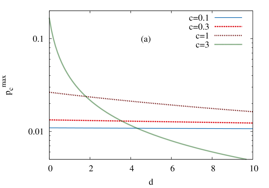
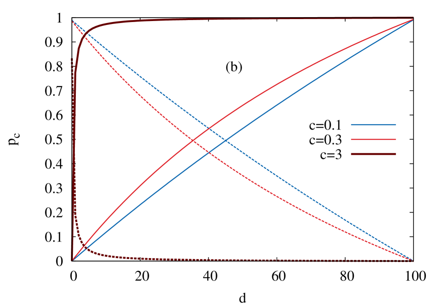
In the RMF model the probability $p^{\text{max}}_{c}(d)$ that a given genotype is a local fitness maximum depends on its distance $d$ to the reference sequence. When the random component is Gumbel distributed this quantity can be computed exactly, with the result

$$p^{\text{max}}_{c}(d)=\frac{1}{1+de^{c}+(L-d)e^{-c}}.$$ (7)

The limits of this expression for small and large $c$

$$p^{\text{max}}_{c}(d) =\begin{cases}\frac{1}{L+1}&c\to 0\\ \delta_{d,0},&c\to\infty\end{cases}$$ (8)

correspond to the HoC model and the additive landscape with a single maximum at $d=0$, respectively. Here the Kronecker symbol $\delta_{x,y}$ is defined by

$$\delta_{x,y} =\begin{cases}1&x=y\\ 0&\textrm{else}.\end{cases}$$ (9)

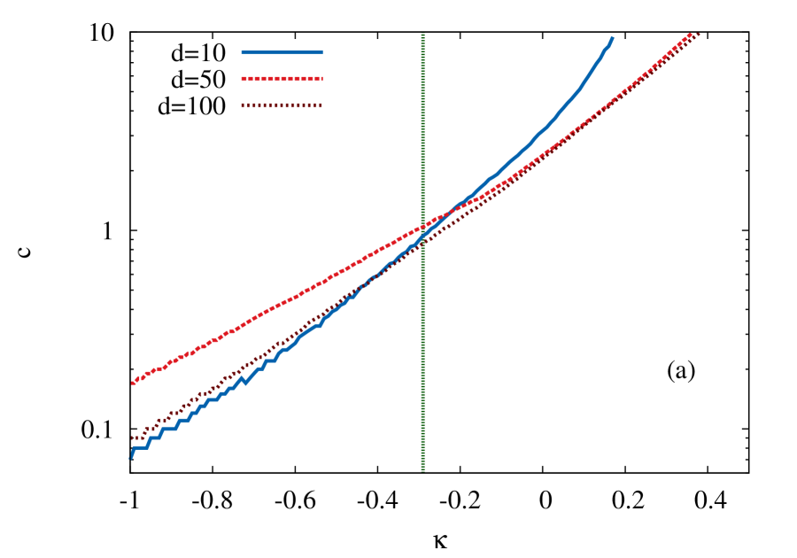
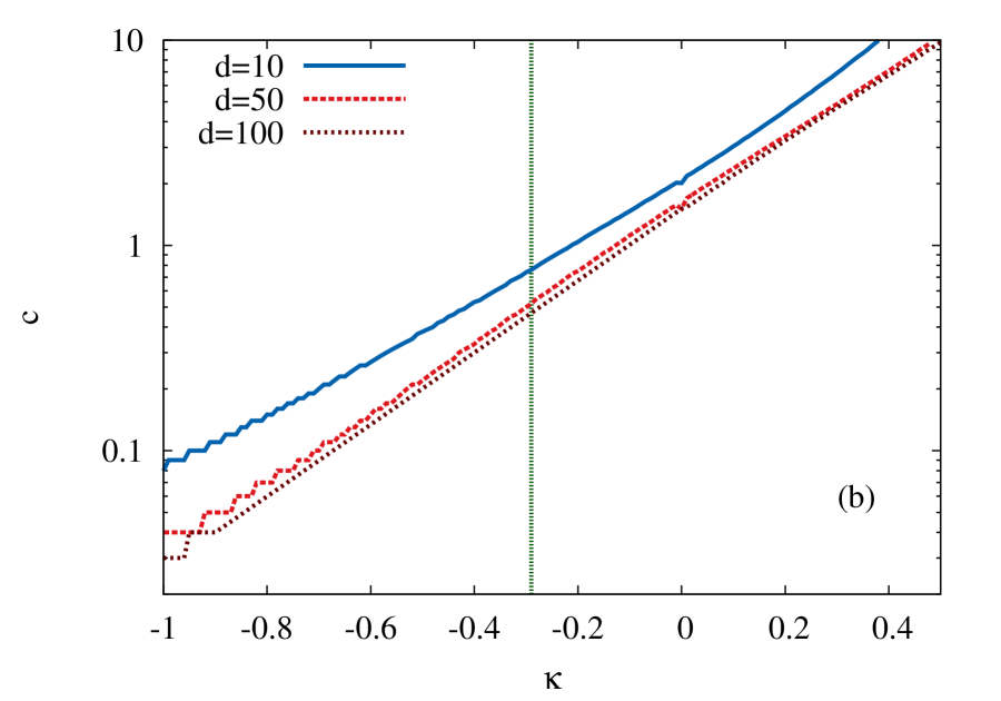
The behavior of (7) for intermediate values of $c$ is illustrated in Figure 1 (a).

It is also of interest to consider the probability that the neighboring genotype of largest fitness for a sequence at distance $d$ from the reference sequence is located in the uphill or downhill part of the neighborhood, denoted by $p_{c}^{\text{up}}(d)$ and $p_{c}^{\text{down}}(d)$, respectively. These probabilities determine the fate of a ‘greedy’ adaptive walk that chooses the neighboring sequence of highest fitness at each step [Orr (2002a]. They can be explicitly evaluated for the Gumbel distribution, with the result

$$p_{c}^{\text{up}}(d)=\frac{d}{d+e^{-c}+e^{-2c}(L-d)},\;\;\;\;\;\;p_{c}^{\text{down}}(d)=\frac{L-d}{L-d+e^{c}+e^{2c}d}.$$ (10)

Note that $p_{c}^{\text{up}}+p_{c}^{\text{down}}+p_{c}^{\text{max}}=1$ and $p_{c}^{\text{up}}=de^{c}p_{c}^{\text{max}}$, $p_{c}^{\text{down}}=(L-d)e^{-c}p_{c}^{\text{max}}$. In the absence of a fitness gradient ($c=0$) the greedy walker is more likely to go uphill (downhill) for $d>L/2$ ($d<L/2$) because of the greater availability of neighboring sequences in that direction. For $c>0$ the crossing point where $p_{c}^{\text{up}}=p_{c}^{\text{down}}$ moves towards the reference sequence and is generally located at $d=\frac{L}{1+e^{2c}}$, see Figure 1b).

Total number of maxima.

Figure 2: (a) The density of local fitness maxima ${\cal{M}}/2^{L}$ in a Gumbel distributed RMF landscape is shown as a function of the number of loci $L$. Symbols correspond to the large $L$ approximation in Equation 13 and lines to the exact expression in Equation A12. The double logarithmic scales illustrate that the ratio ${\cal{M}}/2^{L}$ decays algebraically as $1/L$ for large $L$. (b) The same quantity for an RMF landscape with uniformaly distributed random component, as given by the exact expressions in Equations Weibull class. and Weibull class.. Semi-logarithmic scales are used to illustrate the exponential decay of the ratio ${\cal{M}}/2^{L}$.

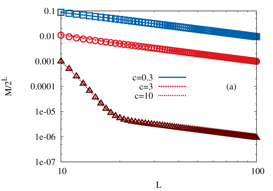
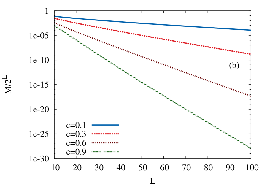
To determine the expected number of local fitness maxima $\mathcal{M}$ in the entire landscape, the distance dependent probability $p_{c}^{\mathrm{max}}(d)$ has to be averaged over $d$ with the appropriate weights giving the number of genotypes at distance $d$,

$$\mathcal{M}=\sum_{d=0}^{L}\binom{L}{d}p^{\text{max}}_{c}(d).$$ (11)

Using the exact expression in Equation 7 for the Gumbel distribution, the sum in Equation 11 can be expressed in terms of a hypergeometric function, see Equation A12. To obtain a more tractable expression we note that for large $L$ the binomial weights in Equation 11 become sharply peaked around $d=\frac{L}{2}$, such that

$$\mathcal{M}\;\stackrel{{\scriptstyle L\to\infty}}{{\approx}}\;2^{L}p_{c}^{\text{max}}(L/2)=\frac{2^{L}}{L\cosh(c)+1}.$$ (12)

For fixed $L$ and large $c$ the expression in Equation 12 violates the obvious bound $\mathcal{M}\geq 1$. A simple modification that cures this deficiency is

$$\mathcal{M}_{\text{approx}}=1+\frac{2^{L}}{L\cosh(c)+1},$$ (13)

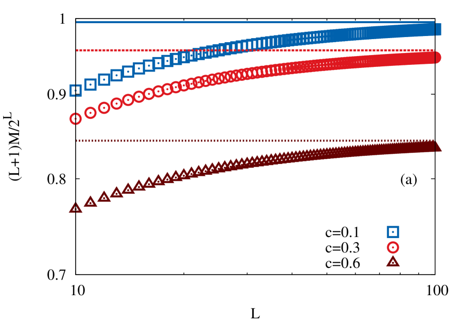
which provides a very good approximation to the exact number of maxima over the entire range of parameters, see Figure 2 (a). Interestingly, apart from a multiplicative constant the large $L$ asymptotics of the number of maxima is the same as for the HoC-model, $\mathcal{M}\sim\frac{2^{L}}{L}$. This is in contrast to the corresponding results for Kauffman’s NK-model, where (depending on how the number of interacting loci $K$ is scaled with the sequence length $L$) different exponential and algebraic dependencies of the number of maxima on $L$ can be found [Perelson and Macken (1995, Evans and Steinsaltz (2002, Durrett and Limic (2003, Limic and Pemantle (2004, Schmiegelt and Krug (2014].

An exact expression for the expected number of maxima is derived in APPENDIX A for exponentially distributed randomness. In that case the asymptotic behavior for large $L$ is seen to be identical to that in Equation 12, and in fact this behavior arises whenever the tail of the distribution is exponential (see Figure A1 (a)). For tails heavier than exponential it is shown that the asymptotics is exactly that of the HoC model, ${\cal{M}}\to\frac{2^{L}}{L}$ independent of $c$, which implies, remarkably, that the mean fitness gradient has no effect on the number of maxima when the genotype dimension is sufficiently large. This result applies in particular to distributions in the Fréchet class of EVT (Figure A1 (b)). For Gumbel-class distributions with tails thinner than exponential the number of maxima is significantly reduced for any value of $c$, and the ratio of $\cal{M}$ to the HoC value $2^{L}/L$ vanishes sub-exponentially in $L$ (see Equation A21).

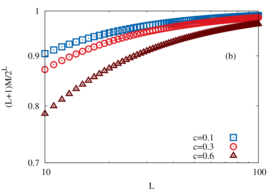
The effect of the mean fitness gradient on the number of local maxima is most pronounced for distributions with bounded support belonging to the Weibull class of EVT. An exact expression for the total number of maxima is derived in APPENDIX A for the case of a uniform fitness distribution, a simple representative of this class, and the result is illustrated in Figure 2 (b). To leading order the number of maxima is proportional to $(2-c)^{L}/L$, which interpolates smoothly between the HoC result for $c=0$ and the additive limit ${\cal{M}}=1$ attained at $c=1$; for $c>1$ the increase in fitness gained in one step towards the reference sequence exceeds the support of the distribution of the random component, and the landscape becomes strictly monotonic in $d$. For other distributions in the Weibull class with support on the the unit interval the behavior is similar, ${\cal{M}}\sim(2-c^{-\frac{1}{\kappa}})^{L}$ to leading order (Equation A26). The behavior of the number of maxima for distributions with bounded support is thus reminiscent of the NK-model at fixed $K$, where it has been shown that ${\cal{M}}\sim\lambda_{K}^{L}$ with a $K$-dependent constant with $1<\lambda_{K}<2$ for $0<K<L-1$ [Durrett and Limic (2003, Limic and Pemantle (2004, Schmiegelt and Krug (2014].

Location of the global maximum.

We next ask where the global maximum is located. For large $c$ it will be found close to the reference sequence $\sigma^{\ast}$, while in the HoC limit $c=0$ it is equally probable to be located anywhere. Since most sequences lie near the distance $L/2$ from the reference sequence, also the global maximum is then most likely at $d=\frac{L}{2}$. In general, the probability for the global maximum to lie at Hamming distance $d$ from the reference sequence is given by

$$P_{\mathrm{max}}(d)=\binom{L}{d}\tilde{P}_{\mathrm{max}}(d),$$ (14)

where $\tilde{P}_{\mathrm{max}}(d)$ is the probability for some specific genotype at distance $d$ to be the globally fittest state and the binomial coefficient accounts for the multiplicity of states at distance $d$. In APPENDIX A it is shown that for the Gumbel distribution

$$\tilde{P}_{\mathrm{max}}(d)=\frac{e^{-cd}}{(1+e^{-c})^{L}}.$$ (15)

With this quantity at hand we proceed to calculate the mean distance of the global maximum from $\sigma^{\ast}$,

$$\mathbb{E}(d)=\frac{L\mathrm{e}^{-c}}{1+\mathrm{e}^{-c}},$$ (16)

which interpolates smoothly between the two limiting cases discussed above, and the corresponding variance

$$\mathrm{Var}(d)=\frac{L\mathrm{e}^{-c}}{(1+\mathrm{e}^{-c})^{2}}.$$ (17)

These calculations could be extended to include the positions of sub-optimal local maxima and thus to address the possible clustering of maxima discussed previously in the context of the NK-model [Kauffman (1993], but we do not pursue this question here. For general distributions an expansion for small $c$ shows that the shift in the position of the maximum from the HoC value $L/2$ is of order $cL2^{-\kappa L}$, where $\kappa$ where $\kappa$ is the extreme value index defined in Equation 4. For distributions in the Weibull class ($\kappa<0$) this implies that minute values of $c\sim 2^{\kappa L}$ suffice to bring the global maximum close to the reference sequence with high probability.

Fitness correlations.

In addition to the number of local maxima, a commonly used measure for fitness landscape ruggedness is the decay of fitness correlations [Weinberger (1990, Stadler and Happel (1999]. Here we consider the correlation function defined by

$$C(r)=\frac{\langle(F(\sigma)-\langle F(\sigma)\rangle)(F(\sigma^{\prime})-\langle F(\sigma^{\prime})\rangle)\rangle_{r}}{\langle(F(\sigma)-\langle F(\sigma)\rangle)^{2}\rangle_{r}}$$ (18)

where angular brackets denote an average over sequence space as well as over the realizations of the random fitness component $\eta$ in Equation 2, and $\langle\cdot\rangle_{r}$ denotes an average over pairs of sequences $\sigma,\sigma^{\prime}$ with $D(\sigma,\sigma^{\prime})=r$. The normalization of the expression in Equation 18 ensures that $C(0)=1$. The derivation in APPENDIX B shows that the correlation function depends on the underlying random fitness distribution only through its variance, and it is given by the expression

$$C_{\text{RMF}}(r)=\frac{\frac{\theta^{2}}{4}(L-2r)+\delta_{r,0}}{\frac{\theta^{2}L}{4}+1}.$$ (19)

The correlation function is a superposition of a peak at $r=0$, which originates from the uncorrelated HoC component in Equation 2, and a linearly decaying piece that reflects the global fitness gradient. It is instructive to compare this result to the correlation function for the NK-model, which reads [Campos et al. (2002, Campos et al. (2003]

$$C_{\text{NK}}(r)=\binom{L}{r}^{-1}\binom{L-K-1}{r}.$$ (20)

This displays a linear decay, $C_{\text{NK}}(r)=1-\frac{r}{L}$, in the non-epistatic limit $K=0$. However, in contrast to Equation 20 which is non-negative for any $r$, Equation 19 becomes negative for $r>\frac{L}{2}$ (see also ?) for further discussion of the relation between the two models).

Adaptation on the RMF landscape

In the previous section we studied properties that depend purely on the topography of the landscape. Now we will shift the focus to the implications of the landscape structure for the evolutionary dynamics. More specifically, we will consider the dynamics in the SSWM limit. Here, only one genotype is populated at any time. If a beneficial mutation occurs, it is either fixed in the entire population or the mutant goes extinct before another mutation arises. Hence, the population behaves as a single entity that performs an ‘adaptive walk’ (AW) on the fitness landscape [Gillespie (1983].

The adaptive walk is a sequence of single adaptive steps. In each step, the population moves from the currently populated sequence to a neighboring one with a transition probability given by the fixation probability normalized by the fixation probabilities of all other available beneficial mutants. Following ?) and ?) we consider the rank-ordered fitness values $F_{j}$ in the current mutational neighborhood, where the rank of the resident genotype is $i$ and beneficial mutants have ranks $j<i$. Since the fixation probabilty of a beneficial mutation in the SSWM regime is proportional to its selection coefficient, the probability for a transition from the current $i$-th fittest genotype to the $j$-th fittest mutant is

$$P_{i\to j}=\frac{F_{j}-F_{i}}{\sum_{k=1}^{i}(F_{k}-F_{i})}.$$ (21)

Based on this expression a number of results have been obtained for the adaptation dynamics on the uncorrelated HoC landscape [Orr (2002b, Rokyta et al. (2006, Joyce et al. (2008]. In the following we ask how these results are modified by the fitness gradient in the RMF model.

A single step of adaptation.

Figure 3: (a) Mean and (b) variance of the fitness rank after an adaptive step in the exponentially distributed RMF landscape is shown as a function of the initial rank. Simulation results for different values of $c$ are compared to the analytical expressions in Equation 22 for the HoC landscape ($c=0$). The good agreement indicates that the properties of single adaptive steps are only weakly affected by the fitness gradient. Here $L=1000$ and $d=50$.

Figure 4: (a) Mean and (b) variance of the fitness rank after an adaptive step in the GPD distributed RMF landscape is shown as a function of the initial rank. Simulation results for different values of $\kappa$ and $c=0.5$ are compared to the analytical expressions in Equation 23 for the HoC landscape, again showing close agreement. Here $L=1000$ and $d=50$.

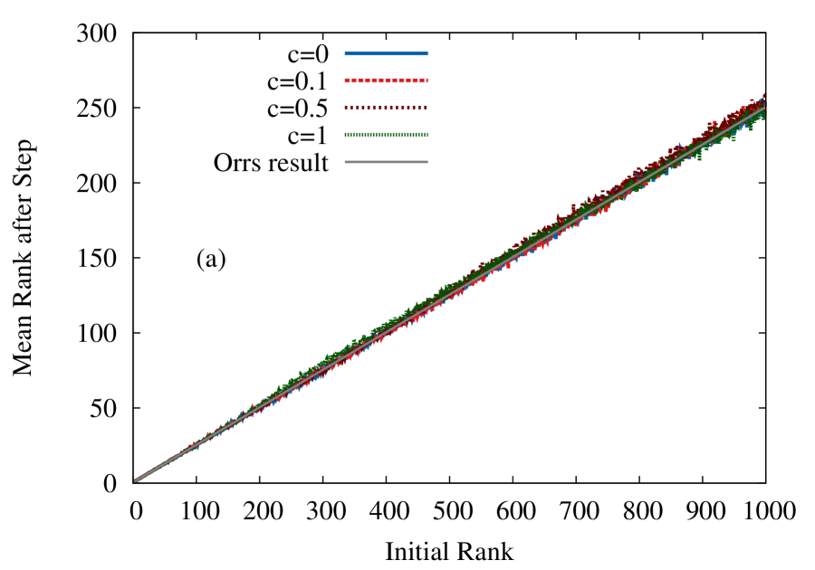
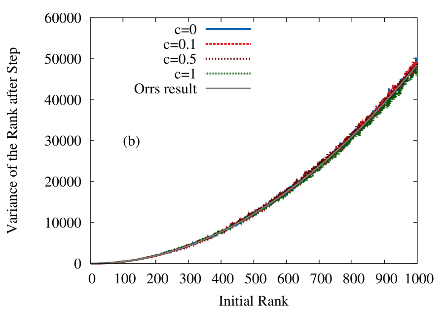
Before we turn to the full adaptive walk we consider a single step of adaptation, specifically the change in the rank of the resident genotype during an adaptive step. Using the transition probability in Equation 21, ?) calculated the expectation value and the variance of the rank $j$ of the next populated sequence after an adaptive step starting from the genotype with rank $i$. For HoC landscapes with fitness values drawn from a Gumbel class distribution he obtained

$$\mathbb{E}(j)=\frac{i+2}{4},\phantom{aaaaaaaaa}\text{Var}(j)=\frac{(i-2)(7i+6)}{144}.$$ (22)

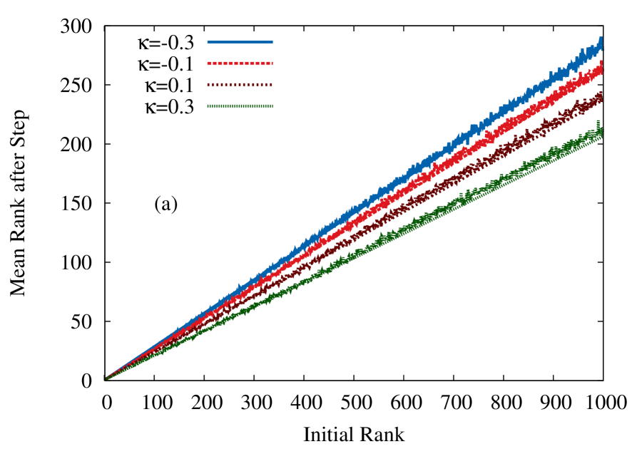
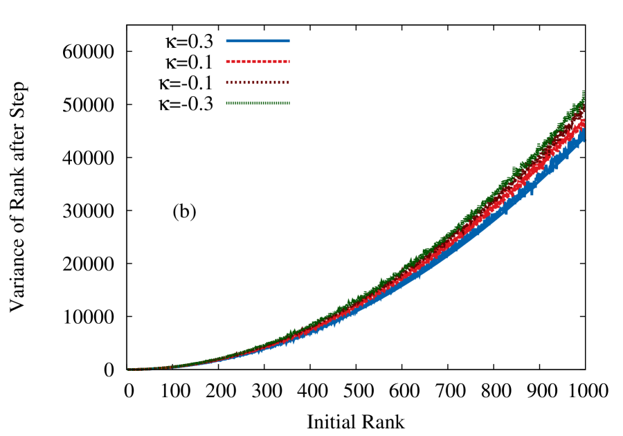
These results were subsequently generalized to the other extreme value classes by ?), who found, for EVT index $\kappa<\frac{1}{2}$,

$$\mathbb{E}(j) =1+\frac{i-2}{2}\left(\frac{1-\kappa}{2-\kappa}\right),$$

$$\text{Var}(j) =\frac{(1-\kappa)(i-2)[(\kappa^{2}-4\kappa+7)i+6(1-\kappa)]}{12(3-\kappa)(2-\kappa)^{2}}.$$ (23)

For $\kappa\to\frac{1}{2}$ the approximation used to derive the expression for $\text{Var}(j)$ breaks down because the fitness distribution ceases to have a second moment; similarly the expression for $\mathbb{E}(j)$ breaks down for $\kappa\to 1$. For further discussion of this case of extremely heavy-tailed fitness distributions we refer to ?).

To see to what extent these results are modified in the RMF landscape we refer to APPENDIX C, where it is shown that the distribution of fitness values in a mutational neighborhood of the RMF model with exponential randomness approximately remains a simple exponential that is shifted by a constant amount depending on the distance $d$ to the reference sequence as well as on the model parameters $c$ and $L$. This implies that the statistics of the fitness spacings $F_{k-1}-F_{k}$ are approximately independent of $c$ and $d$ and take the same form as in the HoC model with exponential fitness distribution. In fact the exponential nature of the fitness spacings in this case is guaranteed by a general theorem of order statistics [Smid and Stam (1975]. Since the transition probability in Equation 21 can be written in terms of these spacings, it seems reasonable to conjecture that the properties of single adaptive steps in the RMF model are well approximated by the HoC results at least for moderate value of the fitness gradient $c$.

To test this conjecture, simulations consisting of the following steps were carried out: (i) create a random RMF neighborhood, (ii) determine the current rank of the initial genotype, (iii) carry out an adaptive step according to Equation 21 and (iv) determine the new rank in the old neighborhood. A comparison of the RMF simulation results to Orr’s analytical formulae in Equation 22 is shown in Figure 3. Obviously, the HoC expressions are in good agreement with the simulation data even in cases where the slope $c$ of the RMF landscape is comparable to the variance $v$ of the random fitness contributions (for the exponential distribution considered here $v=1$).

For other distributions the approximation in APPENDIX C is not directly applicable, but the results shown in Figure 4 indicate that the generalized HoC formulae in Equation 23 provide a good approximation to the RMF model for a range of EVT indices around $\kappa=0$. Thus we conclude, somewhat unexpectedly, that the statistical properties of single adaptive steps are not strongly affected by the fitness gradient in the RMF model.

Adaptive Walks.

Figure 5: Mean length of greedy adaptive walks in an exponentially-distributed RMF landscape with $L=100$, $d=10$. The walk length is independent of starting rank for all $c$.

In the context of AW’s, a property of interest is the mean walk length $\ell$, which is the average number of steps performed until the process reaches a local fitness maximum and terminates. The mean walk length in the HoC landscape has been analyzed using various approaches [Gillespie (1983, Orr (2002b, Flyvbjerg and Lautrup (1992, Neidhart and Krug (2011, Jain and Seetharaman (2011, Jain (2011, Seetharaman and Jain (2014]. Because of the lack of isotropy in the RMF landscapes, analytical results for the walk length are much harder to derive for this model, and the results described in the following were therefore obtained from simulations.

The simulation algorithm is analogous to that described above for the first step of adaptation, but now a new neighborhood is created after each adaptive step and the procedure is repeated until a local maximum has been found, that is, until the current genotype has rank 1 in its new neighborhood. Since the distribution of the fitness values in the new neighborhood depends on the distance to the reference genotype, the direction of the adaptive steps (uphill or downhill) has to be kept track of. Creating the neighborhoods ‘on the fly’ during the adaptive walk implies that the memory of previously visited genotypes is lost beyond the second step. However, the error associated with this approximation is expected to be negligible for large $L$ [Flyvbjerg and Lautrup (1992, Neidhart and Krug (2011] and it is the only feasible approach for simulating walks on landscapes with thousands of loci.

On HoC landscapes the mean walk length is determined primarily by the starting rank $r$, that is, the rank that the first populated state has in its initial neighborhood, and was shown in previous work to be proportional to $\log(r)$ for $r\ll L$, see below for further discussion. On the other hand for a smooth landscape with only one maximum, the walk length equals of course the distance $d$ of the starting point to this maximum. Due to its anisotropic structure, on the RMF landscape one expects the walk length to depend on both initial rank and initial distance to the reference sequence $\sigma^{\ast}$. Specifically, for small $c$ (in the sense $\theta\ll 1$), the mean adaptive walk length should increase logarithmically in the starting rank and be approximately independent of the initial Hamming distance $d$ from $\sigma^{\ast}$, while for $\theta\gg 1$, it should increase linearly in $d$ and be approximately independent of the starting rank, since with high probability only a single maximum exists in the fitness landscape at $\sigma^{\ast}$ or close to it. Analysis of a simplified version of the problem where the walks are assumed to start from the antipode $\overline{\sigma^{\ast}}$ of the reference sequence shows that the two regimes are separated by a sharp transition under certain conditions [Park et al. (2014].

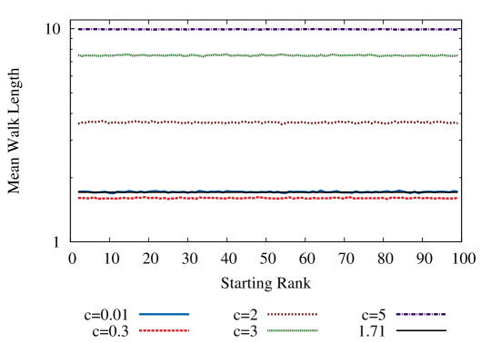
Before discussing the process governed by the transition probability in Equation 21, we briefly consider the simpler case of a greedy adaptive walk in which the transition occurs deterministically to the available genotype of maximal fitness in each step. On HoC landscapes, the mean walk length for this process is known to be asymptotically constant for large $r$ and $L$, approaching the universal limit $\ell=e-1\approx 1.72$ [Orr (2002a]. For the RMF model, simulations displayed in Figure 5 show that for very small $c$, the walk length is still on average equal to $\ell=e-1$. For larger $c$, the mean walk length first decreases slightly (see curve corresponding to $c=0.3$) and then increases rapidly, until $\ell=d$, the limit expected for a smooth landscape. For all values of $c$, the average walk length remains independent of the starting rank.

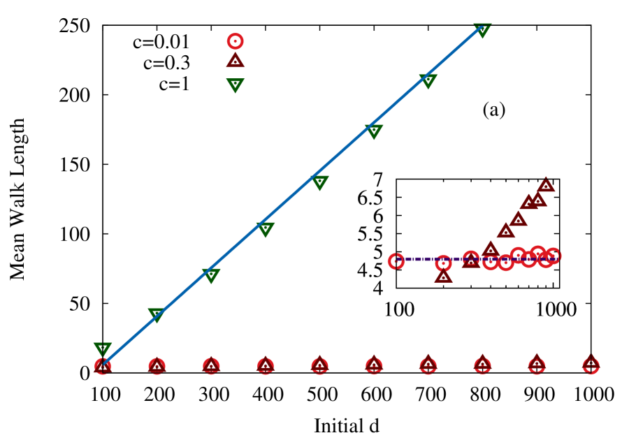
Numerical results obtained from simulations of the full fitness-dependent AW with transition probability in Equation 21 are shown in Figure 6. These simulations were carried out for $L=2000$ loci and the random component of the fitness was drawn from a normal distribution with unit variance. While in the left panel the starting rank was kept constant, the initial Hamming distance to $\sigma^{\ast}$, $d$, was varied. For $c=0.01$ (inset), the behavior seems to be independent of $d$, while a $d$-dependence starts to emerge for $c=0.3$. For $c=1$ the relation between initial distance $d$ and the walk length is roughly linear with a slope smaller than unity.

Figure 6: Mean length of adaptive walks in RMF landscapes with Gaussian randomness. (a) Mean walk length for randomly chosen starting rank versus initial Hamming distance $d$ to the reference sequence. Straight line illustrates the linear dependence of the walk length on $d$ for large $c$. (b) Mean walk length for constant initial Hamming distance $d=1000$ versus starting rank $r$. The horizontal line connecting the data points for $c=1$ illustrates that walk length becomes independent of starting rank for large $c$. Insets show the data for small $c$ on logarithmic scales for $d$ and $r$, respectively. Horizontal line in the inset in panel (a) illustrates that the walk length is independent of initial distance $d$ for $c=0.01$, but acquires such a dependence with increasing $c$. Straight lines in the inset of panel (b) illustrate the logarithmic dependence of the walk length on initial rank for small $c$. The number of loci is $L=2000$.

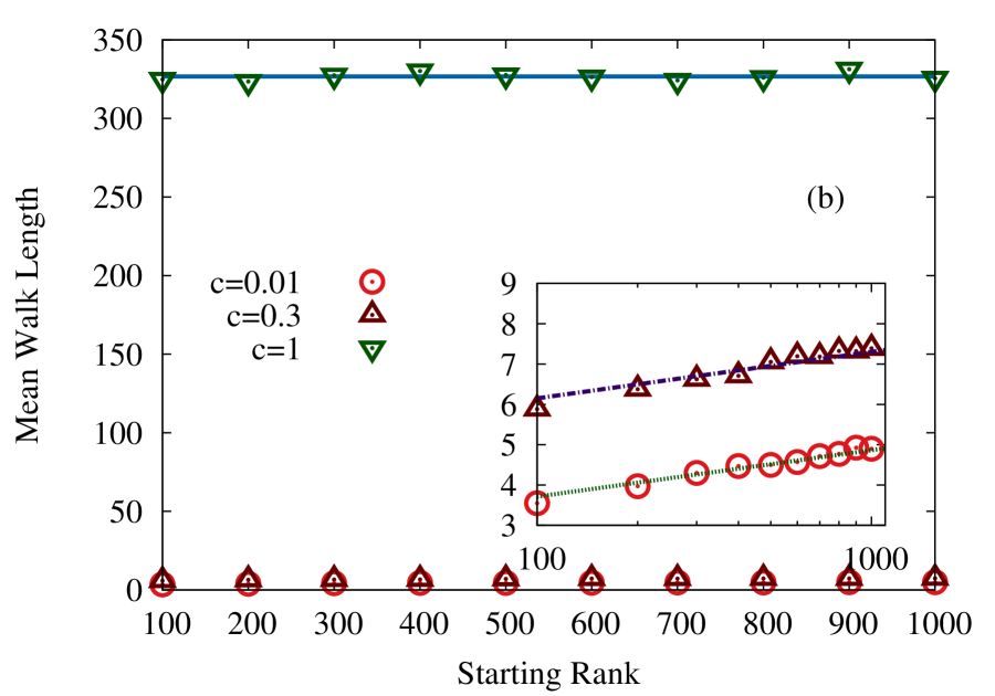
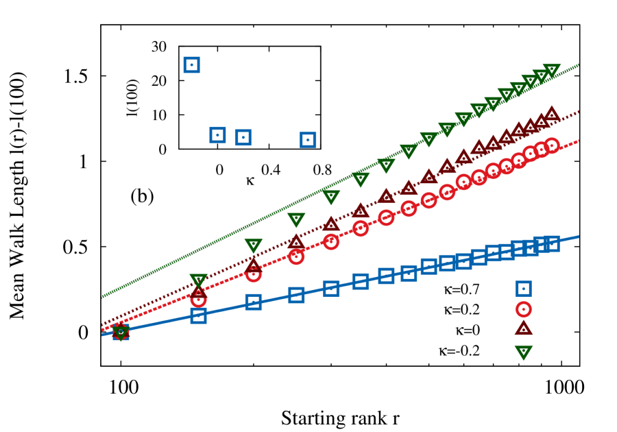
For constant $d=\frac{L}{2}=1000$ and various choices of the starting rank, one can observe the following behavior (Figure 6 (b)). While for $c=1$ the walk length seems to be independent of the starting rank, the data for $c=0.01$ can be fitted by the relation

$$\ell=\frac{1}{2}\log(r)+\text{const.}$$ (24)

which was first obtained by ?) for the HoC landscape with Gumbel-distributed fitness values. For $c=0.3$ the dependence on the starting rank is similar but the constant in Equation 24 is significantly larger.

Equation 24 is a special case of the general relation

$$\ell=\frac{1-\kappa}{2-\kappa}\log(r)+\text{const.}$$ (25)

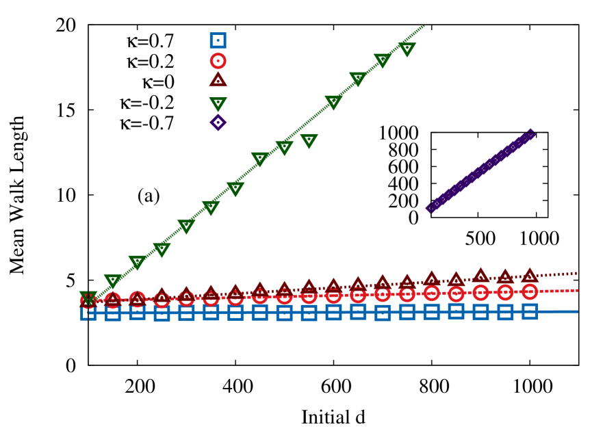
derived by ?) and ?), which holds for HoC landscapes with fitness distributions characterized by an EVT index $\kappa\leq 1$; for $\kappa>1$ the mean walk length is asymptotically independent of starting rank. To see how this behavior is modified in the RMF model, we carried out simulations with the random fitness component drawn from the GPD, keeping $c=0.5$ fixed and varying the EVT index $\kappa$, see Figure 7. The $d$-dependence of the data seems to be well fitted by functions linear in $d$, with a slope that increases rapidly with decreasing $\kappa$ when $\kappa<0$; as was pointed out previously, the effect of the mean fitness gradient is particularly pronounced for distributions in the Weibull class. Somewhat surprisingly, the dependence on the starting rank at fixed $d$ can be approximately described by the functional form in Equation 25 obtained for the HoC model but with a constant depending on $c$ and $\kappa$, see Figure 7 (b).

Figure 7: Mean length of adaptive walks in GPD distributed RMF landscapes for various choices of the EVT index $\kappa$. In both panels $c=0.5$. (a) Walks with randomly chosen starting rank and varying initial Hamming distance $d$ to the reference sequence. Inset shows results for $\kappa=-0.7$, which are off the scale of the main panel. For negative $\kappa$ (Weibull class) the walk length displays a pronounced linear dependence on $d$. (b) Walks starting at constant Hamming distance $d=1000$ and varying starting rank $r$. In the main panel the walk length for $r=100$ has been subtracted for clarity, and the corresponding values of $\ell(100)$ are shown in the inset. The lines in (a) correspond to fits assuming a linear $d$-dependence, lines in (b) show the HoC result in Equation 25. The latter provides a reasonable fit to the data, if a $c$-dependent constant offset is allowed for, but the quality of the approximation gets worse for negative $\kappa$ (Weibull class). The number of loci is $L=2000$.

Summarizing, inspection of the numerical data suggests the following dependencies of the mean adaptive walk length: a linear dependence on $d$ with a slope that increases with increasing $c$ and decreasing $\kappa$, and a logarithmic dependence on the starting rank, similar to that known from the HoC model, with a constant offset depending on $c$, $\kappa$ and $d$. These findings are captured in the following conjectured expression for the adaptive walk length on RMF landscapes:

$$\ell(r,c,d,\kappa)=\frac{1-\kappa}{2-\kappa}\log(r)+\alpha(c,\kappa)d+\beta(c,\kappa)$$ (26)

with so far unknown, nonlinear functions $\alpha,\beta$ with $\alpha(0,\kappa)=0$ and $\beta(0,\kappa)>0$ (see ?) for a discussion of the $\kappa$-dependence of the constant term in Equation 25).

Crossing Probability.

While the adaptive walk length is a measure of the length of typical adaptive trajectories, it is also of interest to ask how likely it is for the population to traverse the entire landscape. To quantify this feature we introduce the crossing probability, which is the probability that an AW starting at the maximal distance $L$ from the reference sequence $\sigma^{\ast}$ reaches it and terminates there. For such an event to happen, three conditions must be fulfilled: The reference sequence $\sigma^{\ast}$ must be a local maximum; there must exist at least one fitness-monotonic path connecting the antipodal sequence $\overline{\sigma^{\ast}}$ to $\sigma^{\ast}$; and finally, such a path must be chosen by the AW. The probability for the first condition was evaluated above and is given by

$$p_{c}^{\mathrm{max}}(0)=\frac{1}{1+Le^{-c}}$$ (27)

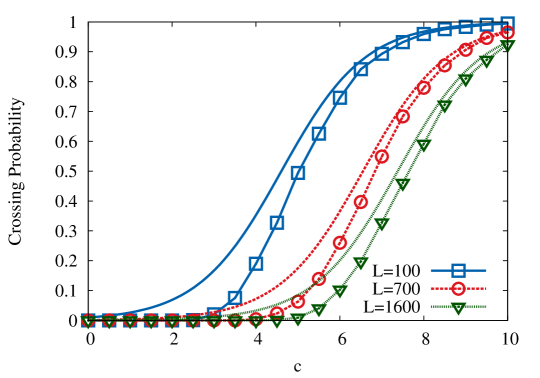
for Gumbel-distributed random fitness component, and this obviously constitutes an upper bound on the crossing probability. The probability for the existence of fitness-monotonic pathways in the RMF model has been investigated previously for the case when the paths end at the global fitness maximum [Franke et al. (2011], and it has been shown that such paths exist with unit probability for large $L$ and any $c>0$ [Hegarty and Martinsson (2014]. It is not clear whether this result applies in the present setting, however, because the probability that the global maximum coincides with the reference sequence vanishes for large $L$ (see Equation A29). Figure 8 shows numerical data for the crossing probability in comparison with the upper bound in Equation 27. Both quantities follow a sigmoidal behavior with a fairly sharp transition from zero to unity around a characteristic value of $c$, which increases roughly logarithmically with $L$, as would be expected on the basis of Equation 27.

Figure 8: The probability for an adaptive walk starting from the antipodal sequence $\overline{\sigma^{\ast}}$ to reach the reference sequence $\sigma^{\ast}$ and terminate there. Results are shown for Gumbel-distributed random fitness components. Numerical results are displayed by symbols connected with lines, while the corresponding lines without symbols show the upper bound given in Equation 27.

The Number of Exceedances

In this section we consider a feature of the fitness landscape that provides a distribution-free statistical test of the assumption of the MLM that fitness values of different genotypes are i.i.d. random variables [Miller et al. (2011]. To define the quantity of interest, suppose that an adaptive step is taken from a starting genotype $\sigma$ with rank $i$ in its neighborhood $\nu(\sigma)$ to a genotype $\sigma^{\prime}$ with rank $j<i$ in $\nu(\sigma)$. The number of exceedances (NoE) is then equal to the number of neighboring genotypes in $\nu(\sigma^{\prime})$ that are fitter than $\sigma^{\prime}$, that is, the rank of $\sigma^{\prime}$ in its own neighborhood minus one. Since the only sequences present in both neighborhoods $\nu(\sigma)$ and $\nu(\sigma^{\prime})$ are $\sigma$ and $\sigma^{\prime}$, the NoE can principally vary between $0$ and $L-1$. Under the HoC assumption that fitness values are i.i.d. random variables, a classic result due to ?) states that the distribution of the NoE is independent of the fitness distribution, and for large $L$ the mean NoE is equal to the rank of $\sigma^{\prime}$ in the initial neighborhood $\nu(\sigma)$ [Rokyta et al. (2006]. In other words, if the first adaptive step goes to a genotype of rank $j$, the expected number of beneficial mutations available for the second step is $j$. In contrast, in a purely additive landscape such as the RMF model for very large $\theta$, the NoE of a genotype is equal to its distance $d$ from the global fitness maximum and independent of its rank in the initial neighborhood.

In their evolution experiments with the microvirid bacteriophage ID11, ?) identified 9 beneficial second step mutations on the background of a mutation, named g2534t, that had been found to have the largest effect among 16 beneficial first step mutants. In order to apply the result of ?), the rank of this mutation among all possible first step mutations (not only the 16 observed in the experiment) has to be estimated. Assuming conservatively that the rank of g2534t among all beneficial first step mutations is at most 3, at most 3 beneficial second step mutations would then have been expected if fitness values were identically and independently distributed. Thus, the observation of 9 beneficial second step mutations allowed ?) to reject the HoC hypothesis with high confidence ($P<0.02$).

Here we ask whether the RMF model is capable of yielding predictions for the NoE that are compatible with the experimental findings of ?). Note that, unlike HoC landscapes, RMF landscapes are not isotropic and the NoE will depend on the position of genotypes $\sigma$ and $\sigma^{\prime}$ on the landscape, i.e. their distance to the reference state, and on whether the adaptive step was taken in the uphill or downhill direction. In contrast to the universal result of ?), there will also be a dependence on the probability distribution of fitness values.

Figure 9: Expected number of times that a sequence which had rank $r$ in the old neighborhood is exceeded in fitness in the new neighborhood, when the adaptive step occurred in the (a) uphill or (b) downhill direction. Symbols show simulation results for the RMF model with exponentially distributed random fitness component, and lines show the approximate analytic expression derived in APPENDIX C. In all cases the initial genotype was located at distance $d=50$ from the reference sequence in a landscape with $L=1000$ loci. The limiting values of the NoE are ${\cal{N}}^{\mathrm{up}}={\cal{N}}^{\mathrm{down}}=r$ for the HoC-model ($c=0$) and ${\cal{N}}^{\mathrm{up}}=d$, ${\cal{N}}^{\mathrm{down}}=0$ for a smooth landscape ($c\to\infty$).

In APPENDIX C we present an approximate analytic calculation of the expected NoE for the RMF model, assuming an exponential distribution for the random fitness component. While the complete expressions for the expected NoE displayed in Equations C8 - C13 are fairly complex, for small $c$ they reduce to the simple form

$${\cal{N}}^{\mathrm{up}}\approx 2+(r-1)e^{c},\;\;\;\;{\cal{N}}^{\mathrm{down}}\approx 2+(r-1)e^{-c}.$$ (28)

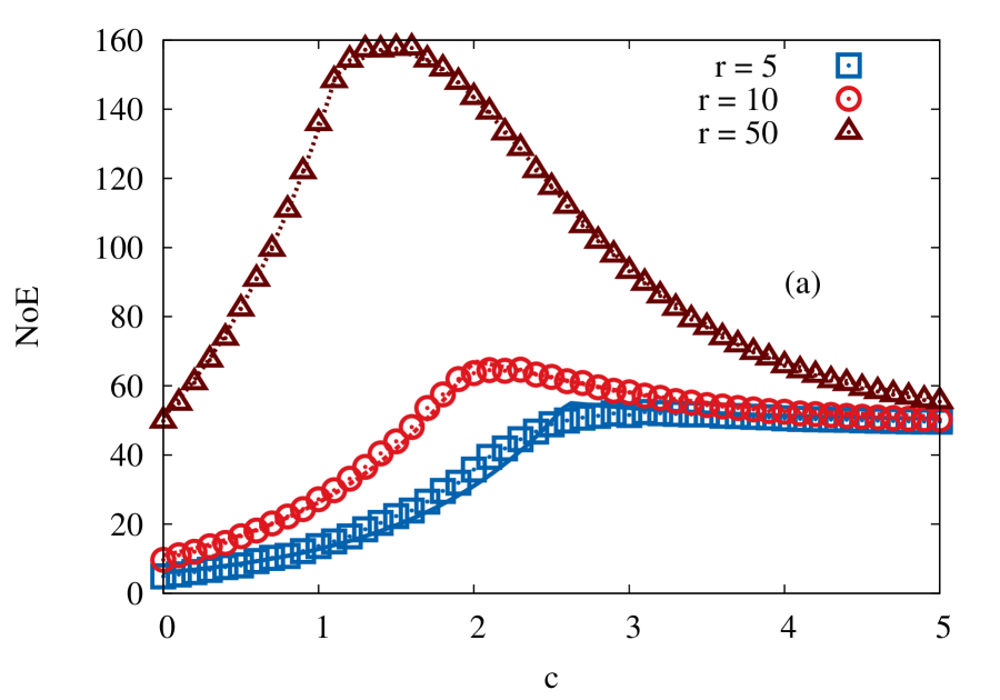
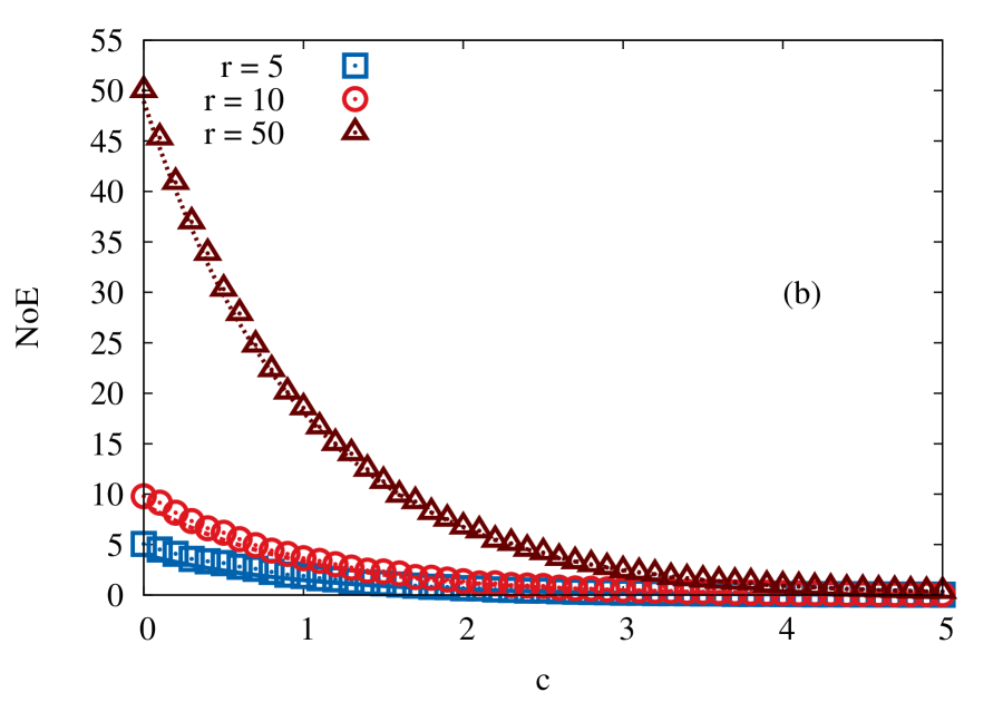
Here ${\cal{N}}^{\mathrm{up}}$ (${\cal{N}}^{\mathrm{down}}$) is the expected number of exceedances after an adaptive step in the uphill (downhill) direction, and $r$ is the rank of the mutated genotype $\sigma^{\prime}$ in the initial neighborhood. For the HoC landscape ($c=0$) Equations 28 yield ${\cal{N}}^{\mathrm{up}}={\cal{N}}^{\mathrm{down}}=r+1$, which differs slightly from the exact result ${\cal{N}}=r$ as a consequence of the approximations involved in the derivation. Figure 9 compares the full expressions derived in APPENDIX C to numerical simulations, showing good agreement. Interestingly, for the case of an uphill step, the expected number of exceedances is maximal for landscapes of intermediate ruggedness.

Figure 10: The figure shows the minimal value of the RMF parameter $c$ required to generate on average 9 exceedances after an adaptive step. Panel (a) shows results for initial rank 1 and panel (b) for initial rank 3. The random fitness component is assumed to be distributed according to the GPD distribution with EVT index $\kappa$, and different curves correspond to different values of the initial distance $d$ to the reference sequence. The experimental estimate $\kappa\approx-0.29$ of the EVT index is indicated by a vertical line. The total number of loci is $L=1000$. Figure C1 shows the same results in a plot where the additive selection coefficient has been scaled by the standard deviation of the distribution of the random component.

Equation 28 shows that a considerable enhancement of the NoE is possible for moderate $c$, provided the adaptive step is in the uphill direction and the random fitness components are exponentially distributed. However, as we do not know whether the beneficial mutations that were observed in the experiments of ?) correspond to uphill or downhill steps in a presumed RMF landscape, we need to average the predictions for the two cases, weighted with the probabilities for each of the two types of transitions to have happened. Furthermore, for an unbiased comparison it is appropriate to consider more general distributions for the random component than the exponential distribution discussed above. Here we choose the GPD distribution, which allows us to cover distributions corresponding to all extreme value classes by varying a single parameter. Extending the approximate derivation in APPENDIX C to this general case is complicated and not very enlightening. Therefore, in the following we use numerical simulations to estimate the NoE.

To find parameter combinations that match the experimentally observed NoE, we constructed RMF landscapes fixing the GPD index in the interval $\kappa\in[-1,0.5]$, and sampling $\kappa$ with a resolution of $\Delta\kappa=0.01$. For each value of $\kappa$, the NoE was calculated for a range of $c$ values. Following ?) we assume that the first step mutation has rank $r=1$ in the initial neighborhood, and determine for each choice of $\kappa$ the smallest value of $c$ for which $\mathcal{N}(1)\geq 9$ (Figure 10 (a)). For comparison, results assuming initial rank $r=3$ are shown in Figure 10 (b). Note that, similar to the case of the exponential distribution displayed in Figure 9, for some $\kappa$ there exists a second, larger $c$ yielding the same value for $\mathcal{N}$. The results displayed in Figure 10 show that the strength of the fitness gradient $c$ required to reproduce the experimentally observed NoE depends sensitively on the EVT index, and becomes very small for negative $\kappa$ deep inside the Weibull domain.

This is in accordance with the generally stronger effect of the additive fitness contribution for negative $\kappa$ discussed above in the context of the statistics of fitness maxima, and reflects the fact that for strongly negative $\kappa$ the random variables drawn from the GPD probability density tend to crowd near the upper boundary of its support. For the EVT index $\kappa=-0.29$ estimated by ?) from a maximum likelihood analysis of the fitness values of 16 first step beneficial mutations, the $c$-value required to produce at least 9 exceedances varies between 0.86 and 1.04 for initial rank 1 and between 0.44 and 0.76 for initial rank 3, depending on the assumed distance $d$ to the reference sequence. Normalizing $c$ by the standard deviation of the random fitness component which equals 0.617 for this value of $\kappa$ (compare to Equation C14), this translates into the intervals $1.39\leq\theta\leq 1.69$ and $0.71\leq\theta\leq 1.23$ for the parameter $\theta$, respectively, which in comparison to estimates for other empirical data sets is indicative of a relatively smooth landscape. To further narrow down the range of RMF model parameters that can provide a consistent description of the fitness landscape of the ID11 microvirid system would require including other experimental observables into the analysis, which is beyond the scope of this article.

Discussion

Motivated by the increasing availability of empirical information about the structure of adaptive landscapes, we have presented a detailed analysis of a one-parameter family of tunably rugged fitness landscapes. The model is a variant of the Rough Mount Fuji landscape, in which the locus-specific additive effects considered in the original version [Aita et al. (2000, Aita and Husimi (2000] are replaced by a single parameter, and ruggedness is governed by the ratio $\theta$ of the additive fitness effect to the standard deviation of the random fitness component.

Landscape topography.

The mathematical simplicity of the model allowed us to derive several explicit results for the number and positions of local and global maxima; such results are much harder to come by for other generic fitness landscape models, notably Kauffman’s NK-model. In particular, we have arrived at a complete classification of the expected number of fitness maxima in the limit of large genotype dimensionality $L$, which highlights the importance of the tail behavior of the distribution of the random fitness component in determining the ruggedness of the landscape. For distributions with tails heavier than exponential, the additive fitness component becomes asymptotically irrelevant, in the sense that the number of maxima is equal to the value expected for an uncorrelated HoC landscape. In contrast, for distributions with bounded support the number of maxima is reduced compared to the HoC expectation by a factor that varies exponentially in $L$. The interplay between additive effects and tail behavior has been a recurrent theme of this article which manifests itself in various quantities of interest. Our results show that both the parameter $\theta$ characterizing the additive effects and the EVT index $\kappa$ must be specified for a comprehensive description of the landscape topography in the RMF model.

An exception to this rule is provided by the fitness correlation function which, similar to the NK-model, is independent of the type of randomness. In contrast to the NK-model, however, the correlations become negative at large distances, which reflects the inherent anisotropy of the RMF landscape and the long-range effect of the fitness gradient.

Another important measure of fitness landscape ruggedness not discussed so far in this article is the existence and abundance of selectively accessible mutational pathways, defined as paths composed of single mutational steps along which fitness increases monotonically [Weinreich et al. (2006, Franke et al. (2011]. Using an approach similar to that of the present work, an explicit expression for the expected number of accessible pathways in the RMF model with Gumbel-distributed randomness can be derived [Franke et al. (2010, Franke et al. (2011]. Subsequently ?) presented a rigorous proof that accessible pathways exist with unit probability for large $L$ in the RMF model for any $c>0$, independent of the distribution of the random fitness component. This is in stark contrast to the behavior in the HoC model ($c=0$), where the probability for existence of accessible paths tends to zero for large $L$. Analyses in which the genotypes are placed on a regular tree show that this strong dichotomy between the HoC and RMF models is specific to the hypercube topology of sequence space [Nowak and Krug (2013, Roberts and Zhao (2013].

Dynamics of adaptation.

Apart from being amenable to rigorous analysis, the RMF model is useful for exploring various aspects of evolutionary dynamics in rugged fitness landscapes through simulations. Recent applications in this context include studies of evolutionary predictability [Lobkovsky et al. (2011, Szendro, Franke et al. (2013], epistatic interactions between mutations occurring along an adaptive walk [Greene and Crona (2014] and the effect of recombination on rugged fitness landscapes [Nowak et al. (2014]. Here we have focused on adaptation in the SSWM regime and considered both single adaptive steps and adaptive walks to local fitness maxima. Interestingly, while the statistics of single adaptive steps largely conforms to the classic results obtained for the MLM [Orr (2002b, Joyce et al. (2008], adaptive walks in the RMF are much longer than in the MLM already for small values of $c$. Specifically, the heuristic expression in Equation 26 that summarizes the simulation results suggest a linear dependence of the walk length on the initial distance to the reference sequence.

The qualitatively different effects that the fitness correlations in the RMF have on single vs. multiple adaptive steps highlight the fact that a step in an adaptive walk involves two distinct random processes [Rokyta et al. (2006, Neidhart and Krug (2011]. The first process is the selection of a fitter neighbor according to the transition probability in Equation 21, and the second process is the change of the mutational neighborhood after the fixation of the mutated genotype. In the MLM the effect of the second process is relatively weak, and as a consequence adaptive walks are well described by an approximation which ignores the neighborhood change [Orr (2002b, Neidhart and Krug (2011].

To understand the role of the neighborhood change in the RMF model we refer to the analysis in APPENDIX C, where it is shown (for exponentially distributed randomness) that the effect of the fitness gradient can be approximately subsumed into an overall shift of all the fitness values constituting a neighborhood by the same amount. This implies that the transition probability in Equation 21, which depends only on fitness differences within the neighborhood, is approximately independent of $c$. However, since the shift is a function of the distance $d$ to the reference sequence which changes in the adaptive step, the rank of the mutant genotype in the new neighborhood is strongly dependent on whether the step occurred in the uphill ($d\to d-1$) or downhill ($d\to d+1$) direction. Further investigations are required to elucidate how this effect gives rise to the observed dependence of the walk length on the landscape parameters. A promising approach is to consider walks starting from the antipode of the reference sequence, which can be assumed to move almost exclusively in the uphill direction provided the walk length remains short compared to $L$ [Park et al. (2014].

For large populations and/or high mutation rates the SSWM approximation underlying the simple adaptive walk picture breaks down, and additional processes such as the competition between beneficial clones and the crossing of fitness valleys have to be taken into account. The resulting complex population dynamics is governed by the tension between a tendency towards greater determinism induced by clonal competition [Jain and Krug (2007, Jain et al. (2011] and the increasing role of non-monotonic pathways that become accessible through valley crossing [Szendro, Franke et al. (2013, de Visser and Krug (2014]. In contrast to the SSWM regime, the trapping of large populations at local fitness maxima is only a transient occurrence, and the rate of escape from such peaks plays an important role in the comparison between recombining and non-recombining populations on rugged fitness landscapes [Nowak et al. (2014].

Application to experiments.

The usefulness of the RMF model for the quantitative description of empirical fitness landscapes has been documented in several recent studies. ?) applied the model to an 8-locus fitness landscape for the fungus Aspergillus niger, and extracted an estimate of $c$ from a subgraph analysis of pathway accessibility. In a study of amplitude spectra of fitness landscapes ?) showed that the correlation function of a 6-locus fitness landscape obtained by ?) for the yeast Saccharomyces cerevisiae is well described by the RMF model. Lastly, in a meta-analysis of 10 empirical fitness landscapes ?) used the RMF model to interpolate the behavior of various ruggedness measures between the limits of a completely random (HoC) and an additive landscape, and found good agreement with the trends in the empirical data.

In the present article we have complemented these analyses by considering the effect that the fitness gradient in the RMF model has on the number of secondary beneficial mutations that are available after an adaptive step. We have identified model parameters for which the RMF prediction matches the large number of fitness exceedances observed in the experiment of ?). A small fitness gradient suffices to explain the experiments when the distribution of the random fitness component is assumed to belong to the Weibull class of EVT, as is suggested by the analysis of the distribution of first-step mutational effects. We believe that more work along these lines, focusing on the changes in the statistics of mutational neighborhoods along an adaptive trajectory, will provide important insights into the role of epistatic interactions during adaptation and the viability of schematic models like the one considered here.

Appendix A: Properties of fitness maxima

Density of local maxima.

The probability $p^{\text{max}}_{c}(d)$ that a genotype at distance $d$ from the reference sequence is a local fitness maximum is given by the integral

$$p^{\text{max}}_{c}(d) =\int dx\;p(x)\left(P(x-c)\right)^{d}\left(P(x+c)\right)^{L-d}.$$ (A1)

This is simply the probability that the genotype’s fitness $x$ exceeds that of its uphill and downhill neighbors, averaged with respect to the probability density $p(x)$. Unless specified otherwise, here and in the following the domain of integration is equal to the support of the probability distribution. For the Gumbel distribution $P_{G}(x)=e^{-e^{-x}}$ the integral (A1) can be evaluated exactly using the shift property (6), yielding the result in Equation 7 of the main text.

Similarly, the probabilities to find the neighboring genotype of largest fitness in the uphill or downhill direct, respectively, are given by

$$p_{c}^{\text{up}}(d) =d\int dx\;p(x)P(x)^{d-1}P(x+c)P(x+2c)^{L-d},$$ (A2)

$$p_{c}^{\text{down}}(d) =(L-d)\int dx\;p(x)P(x)^{L-d-1}P(x-c)P(x-2c)^{d},$$ (A3)

which can be evaluated for the Gumbel distribution to yield the expressions in Equation 10.

Total number of maxima.

Inserting Equation A1 into the sum in Equation 11 and exchanging the order of integration and summation one arrives at the compact expression

$${\cal{M}}=\int dx\;p(x)[P(x-c)+P(x+c)]^{L}$$ (A4)

which will be evaluated in the following for various special cases. Equation A4 makes it evident that ${\cal{M}}$ is an even function of $c$: Changing $c$ to $-c$ produces a fitness landscape with the antipodal reference sequence $\overline{\sigma^{\ast}}$ that is statistically equivalent to the original landscape.

Exponential distribution.

For the exponential distribution defined by

$$P(x) =\begin{cases}1-e^{-x}&x\geq 0\\ 0&x<0\end{cases}$$ (A5)

the expression in Equation A4 becomes

$${\cal{M}}=\int_{0}^{c}dx\;e^{-x}[1-e^{-c}e^{-x}]^{L}+2^{L}\int_{c}^{\infty}dx\;e^{-x}[1-\cosh(c)e^{-x}]^{L}.$$ (A6)

Substituting $z=e^{-x}$ this yields

$${\cal{M}}=\int_{e^{-c}}^{1}dz\;[1-e^{-c}z]^{L}+2^{L}\int_{0}^{e^{-c}}dz[1-\cosh(c)z]^{L}=$$

$$\frac{e^{c}}{L+1}\left[(1-e^{-2c})^{L+1}-(1-e^{-c})^{L+1}\right]+\frac{2^{L}}{\cosh(c)(L+1)}\left[1-(1-e^{-c}\cosh(c))^{L}\right].$$ (A7)

It is straightforward to check that ${\cal{M}}\to 1$ for $c\to\infty$. Moreover, the asymptotics for large $L$ at fixed $c$ is identical to that derived in Equation 12 for the Gumbel distribution, ${\cal{M}}\sim\frac{2^{L}}{L\cosh(c)}$.

Gumbel distribution.

Inserting the exact expression in Equation 7 into Equation 11 one obtains

$$\mathcal{M}=\sum_{d=0}^{L}\binom{L}{d}\frac{1}{1+de^{c}+(L-d)e^{-c}}.$$ (A8)

We first show that the sum in Equation A8 can be expressed in terms of a hypergeometric function defined by [Graham et al. (1994]

$$\,{}_{2}F_{1}(a,b;c;z) =\sum_{n\geq 0}\frac{(a)_{n}(b)_{n}}{(c)_{n}}\,\frac{z^{n}}{n!}=\sum_{n\geq 0}t_{n}$$

where the Pochhammer symbol is defined by

$$(x)_{n}=\left\{\begin{array}[]{ll}1&\mbox{if }n=0\\ x(x+1)\cdots(x+n-1)&\mbox{if }n>0.\end{array}\right.$$

The defining feature of the hypergeometric function is that the terms $t_{n}$ satisfy $t_{0}=1$ and

$$\frac{t_{k+1}}{t_{k}}=\frac{(k+a)(k+b)}{k+c}\frac{z}{k+1}.$$ (A9)

To bring Equation A8 into this form we write

$$\mathcal{M}=\frac{1}{1+Le^{-c}}\sum_{d\geq 0}\binom{L}{d}p^{\text{max}}_{c}(d)(1+Le^{-c}),$$ (A10)

ensuring that $t_{0}=1$, and compute the fractions $t_{d+1}/t_{d}$ according to

$$\frac{t_{d+1}}{t_{d}}=\left(\frac{L-d}{d+1}\right)\frac{1+Le^{-c}+2d\sinh(c)}{1+Le^{-c}+2(d+1)\sinh(c)}=\left(\frac{-1}{d+1}\right)\frac{(d-L)\left(d+\frac{1+Le^{-c}}{2\sinh(c)}\right)}{d+1+\frac{1+Le^{-c}}{2\sinh(c)}}.$$ (A11)

By comparison with Equation A9 the arguments $a,b,c$ and $z$ can be identified and it follows that

$$\mathcal{M}=(1+Le^{-c})^{-1}\;{{}_{2}F_{1}}(-L,\zeta;\zeta+1;-1)\;\;\;\text{with}\;\;\;\zeta=\frac{1+Le^{-c}}{2\sinh c}.$$ (A12)

The asymptotic behavior for large $L$ is most conveniently extracted from the general expression in Equation A4, which in this case can be brought into the form

$${\cal{M}}=\int_{0}^{1}dP\;[P^{e^{c}}+P^{e^{-c}}]^{L}.$$ (A13)

Recognizing that the dominant contribution to the integral comes from the region near $P=1$ and expanding the integrand around this point one readily finds that ${\cal{M}}\approx\frac{2^{L}}{L\cosh(c)}$ for large $L$, in agreement with Equation 12. Along similar lines it can be shown that the same asymptotics obtains for any distribution with a strictly exponential tail.

Fréchet class.

Here we show that for distributions in the Fréchet class the expected number of maxima is asymptotically equal to that in the HoC model, ${\cal{M}}\approx\frac{2^{L}}{L}$, for large $L$ and any $c>0$. To simplify the notation we use a standard Pareto distribution defined by

$$P(x) =\begin{cases}1-x^{-\alpha}&x\geq 1\\ 0&x<1\end{cases}$$ (A14)

where the exponent $\alpha$ is related to the EVT index through $\alpha=\frac{1}{\kappa}$. Similar to the case of the exponential distribution, the domain of integration in Equation A4 has to be subdivided into the interval $[1,1+c)$, where $P(x-c)=0$, and the remainder $[1+c,\infty)$. The dominant contribution comes from the second part, which is given by

$$\mathcal{M}\approx 2^{L}\int_{1+c}^{\infty}dx\;\alpha x^{-(\alpha+1)}\left[1-\frac{1}{2}[(x+c)^{-\alpha}+(x-c)^{-\alpha}]\right]^{L}$$

$$\approx 2^{L}\int_{1+c}^{\infty}dx\;\alpha x^{-(\alpha+1)}\exp\left[-\frac{1}{2}Lx^{-\alpha}[(1+c/x)^{-\alpha}+(1-c/x)^{-\alpha}]\right]$$ (A15)

for large $L$. Substituting $y=Lx^{-\alpha}$ this yields

$$\mathcal{M}\approx\frac{2^{L}}{L}\int_{0}^{\frac{L}{(1+c)^{\alpha}}}dy\;\exp\left[-\frac{y}{2}[(1+c(y/L)^{1/\alpha})^{-\alpha}+(1-c(y/L)^{1/\alpha})^{-\alpha}]\right]\to\frac{2^{L}}{L}$$ (A16)

as claimed.

Figure A1: Expected number of maxima $\cal{M}$ normalized by its asymptotic value for a HoC landscape, $\frac{2^{L}}{L}$. Panel (a) shows the exact result in Equation Exponential distribution. for an exponentially distributed random contribution. Dashed horizontal lines illustrate that the ratio converges to $\frac{1}{\cosh(c)}$ for large $L$. Panel (b) shows a numerical evaluation of Equation 11 for a Pareto distributed random contribution with $\alpha=2$ ($\kappa=\frac{1}{2}$). In accordance with Equation A16 the ratio converges to unity for large $L$.

Gumbel class.

We are now in the position to generalize the results obtained for the exponential and Gumbel distributions to the entire Gumbel class of EVT. For calculational convenience we choose the one-parameter family of Weibull distributions defined by

$$P(x) =\begin{cases}1-\exp[-x^{\beta}]&x\geq 0\\ 0&x<0\end{cases}$$ (A17)

to represent Gumbel-class distributions with tails that are heavier (for $\beta<1$) or lighter (for $\beta>1$) than exponential. As in the cases considered above, the dominant contribution to the number of maxima comes from the part of the integral in Equation A4 that extends from $c$ to infinity, which now reads

$$\mathcal{M}\approx 2^{L}\int_{c}^{\infty}dx\;p(x)\left[1-\frac{1}{2}[e^{-(x+c)^{\beta}}+e^{-(x-c)^{\beta}}]\right]^{L}.$$ (A18)

The crucial difference between the cases $\beta<1$ and $\beta>1$ lies in the behavior of the ratio of the two exponential terms inside the inner square brackets. For $\beta<1$

$$\lim_{x\to\infty}\frac{e^{-(x+c)^{\beta}}}{e^{-(x-c)^{\beta}}}=1$$ (A19)

which implies that the shift by $\pm c$ becomes irrelevant asymptotically and ${\cal{M}}\to\frac{2^{L}}{L}$ independent of $c$, as in the Fréchet class. On the other hand, for $\beta>1$ one finds that $e^{-(x-c)^{\beta}}\gg e^{-(x+c)^{\beta}}$ for large $x$ and Equation A18 simplifies to

$$\mathcal{M}\approx 2^{L}\int_{c}^{\infty}dx\;p(x)\left[1-\frac{1}{2}e^{-(x-c)^{\beta}}\right]^{L}\approx 2^{L}\int_{c}^{\infty}dx\;p(x)\exp\left[-\frac{L}{2}e^{-(x-c)^{\beta}}\right].$$ (A20)

For large $L$ the integrand is effectively zero below a cutoff scale $x^{\ast}$ determined by $Le^{-(x-c)^{\beta}}\sim 1$ or $x^{\ast}\approx c+(\ln L)^{1/\beta}$. Thus

$$\mathcal{M}\approx 2^{L}[1-P(x^{\ast})]=2^{L}\exp[-(c+(\ln L)^{1/\beta})^{\beta}]\approx\frac{2^{L}}{L}\exp[-\beta c(\ln L)^{1-\frac{1}{\beta}}]$$ (A21)

to leading order in $L$.

Weibull class.

We next consider distributions with bounded support, which we take to be the unit interval $[0,1]$. In the evaluation of the general expression in Equation A4 it has to be taken into account that $P(x-c)=0$ for $x<c$ and $P(x+c)=1$ for $x>1-c$, which implies in particular that the cases $c<\frac{1}{2}$ (where $c<1-c$) and $c>\frac{1}{2}$ (where $c>1-c$) have to distinguished. We begin with the uniform distribution and assume $c<\frac{1}{2}$, which yields

$$\mathcal{M}=\int_{0}^{c}dx\;(x+c)^{L}+\int_{c}^{1-c}dx\;(2x)^{L}+\int_{1-c}^{1}dx\;(1+x-c)^{L}$$

$$=\frac{1}{L+1}[(2-c)^{L+1}+(2^{L}-1)c^{L+1}-2^{L}(1-c)^{L+1}].$$ (A22)

Analogously for $c>\frac{1}{2}$ we obtain

$$\mathcal{M}=\int_{0}^{1-c}dx\;(x+c)^{L}+\int_{1-c}^{c}dx\;+\int_{c}^{1}dx\;(1+x-c)^{L}$$

$$=\frac{1}{L+1}[(2-c)^{L+1}-c^{L+1}]+2c-1.$$ (A23)

Comparing Equations Weibull class. and Weibull class. the two expressions are seen to conincide at $c=\frac{1}{2}$. Moreover, Equation Weibull class. reduces to $\frac{2^{L}}{L+1}$ for $c=0$ and Equation Weibull class. confirms that ${\cal{M}}=1$ for $c=1$, as expected.

As representatives of Weibull-class distributions with a general EVT index $\kappa<0$ we consider the Kumaraswamy distributions defined by

$$P(x) =\begin{cases}1-(1-x)^{\nu}&0\leq x\leq 1\\ 0&x<0\\ 1&x>1\end{cases}$$ (A24)

with $\nu=-\frac{1}{\kappa}$. We focus on the leading order behavior of the number of maxima for large $L$, which is given by the part of the integral in Equation A4 that contains the upper boundary of the support at $x=1$ (compare to Equations Weibull class. and Weibull class.). We assume $c<\frac{1}{2}$ and obtain

$$\mathcal{M}\approx 2^{L}\int_{1-c}^{1}dx\;\nu(1-x)^{\nu-1}\left[1-\frac{1}{2}(1-x+c)^{\nu}\right]^{L}=2^{L}\int_{0}^{c}dy\;\nu y^{\nu-1}\left[1-\frac{1}{2}(y+c)^{\nu}\right]^{L},$$ (A25)

which is dominated by the region near $y=0$ for large $L$. Expanding $(y+c)^{\nu}$ for small $y$ it follows that

$$\mathcal{M}\approx(2-c^{\nu})^{L}\int_{0}^{c}dy\;\nu y^{\nu-1}\exp\left[-\frac{\nu c^{\nu-1}Ly}{2-c^{\nu}}\right]\to\frac{\nu\Gamma(\nu)}{(\nu c^{\nu-1})^{\nu}}\frac{(2-c^{\nu})^{L+\nu}}{L^{\nu}}$$ (A26)

for large $L$, where $\Gamma$ denotes the Gamma-function. The result for $c>\frac{1}{2}$ is asymptotically the same. Thus to leading order the number of maxima is ${\cal{M}}\sim\frac{(2-c^{-\frac{1}{\kappa}})^{L}}{L^{-\frac{1}{\kappa}}}$ in the Weibull class.

Expansion for small $c$.

A unified view of the effect of the fitness gradient on the expected number of maxima can be obtained by expanding the general expression in Equation A4 for small values of $c$. To leading order in $c$ the integrand is $P(x-c)+P(x+c)=2P(x)+c^{2}P^{\prime\prime}(x)=2P(x)+c^{2}p^{\prime}(x)$, where primes indicate derivatives with respect to $x$. Integrating and keeping terms of order $c^{2}$ we thus obtain

$${\cal{M}}=\frac{2^{L}}{L+1}-2^{L-2}L(L-1)c^{2}\int dx\;p(x)^{3}P(x)^{L-2}+{\cal{O}}(c^{4}).$$ (A27)

Evaluating the integral on the right hand side for the GPD distribution in Equation 4 one finds that it is of the order of $L^{-(3+2\kappa)}$, and hence the entire correction term is of order $2^{L}L^{-(1+2\kappa)}c^{2}$. Thus for $\kappa>0$ (Fréchet class) the correction becomes negligible compared to the HoC term for large $L$. In contrast, for $\kappa<0$ (Weibull class) the correction term eventually dominates the HoC term, showing that the leading order behavior of ${\cal{M}}$ is modified.

Location of the global maximum.

To compute the probability $\tilde{P}_{\mathrm{max}}(d)$ that a sequence at distance $d$ is the global fitness maximum one has to demand that its fitness exceeds the fitnesses of all other sequences, which leads to the expression

$$\tilde{P}_{\mathrm{max}}(d)=\int_{-\infty}^{\infty}\mathrm{d}xp(x+cd)\prod_{j=0}^{L}P(x+cj)^{\binom{L}{j}-\delta_{dj}}.$$ (A28)

Inserting the Gumbel distribution in Equation 5 and using its shift property in Equation 6, this can be evaluated according to

$$\tilde{P}_{\mathrm{max}}(d) = \int dy\;p_{G}(y)\prod_{j=0}^{L}P_{G}(y+c(j-d))^{\binom{L}{j}-\delta_{dj}}=\int dy\;p_{G}(y)P_{G}(y)^{\sum_{j=0}^{L}e^{-c(j-d)}\left[\binom{L}{j}-\delta_{dj}\right]}$$ (A29)

$$= \int dy\frac{dP_{G}}{dy}P_{G}(y)^{e^{cd}(1+e^{-c})^{L}-1}=\int_{0}^{1}dz\;z^{e^{cd}(1+e^{-c})^{L}-1}=\frac{e^{-cd}}{(1+e^{-c})^{L}}.$$

For general fitness distributions one has to resort to an expansion in $c$. Starting from Equation A28 and collecting terms linear in $c$ one obtains

$$\tilde{P}_{\mathrm{max}}(d)=\frac{1}{2^{L}}+c2^{L}(L/2-d)I_{2^{L}-2}+\mathcal{O}(c^{2}),$$ (A30)

where

$$I_{L}=\int dx\;p(x)^{2}P(x)^{L}.$$ (A31)

Expressions for $I_{L}$ for representatives of the three extreme value classes have been derived by ?). For large $L$ they behave as [Wergen et al. (2011]

$$I_{L}\sim L^{-(2+\kappa)}.$$ (A32)

The weighted average with respect to $d$ then yields the approximate expression

$$\mathbb{E}(d)\approx\frac{L}{2}-cL2^{2L-2}I_{2^{L}-2}$$ (A33)

for the mean distance of the global maximum to the reference sequence. Using the asymptotic behavior of $I_{L}$ given in Equation A32 it follows that the shift in the position of the maximum from the HoC value $L/2$ is of order $cL2^{-\kappa L}$.

Appendix B: Calculation of the fitness correlation function

For notational convenience we substract the mean value $\mathbb{E}(\eta)$ of the random fitness component from Equation 2 and define

$$f(\sigma)=F(\sigma)-\mathbb{E}(\eta)=-cd+\xi(\sigma)\;\;\;\text{with}\;\;\;\xi(\sigma)=\eta(\sigma)-\mathbb{E}(\eta),$$ (B1)

such that $\mathbb{E}(\xi)=0$. It is then easy to see that

$$\langle(F(\sigma)-\langle F(\sigma)\rangle)(F(\sigma^{\prime})-\langle F(\sigma^{\prime})\rangle)\rangle_{r}=\langle(f(\sigma)-\langle f(\sigma)\rangle)(f(\sigma^{\prime})-\langle f(\sigma^{\prime})\rangle)\rangle_{r}=c^{2}[\langle dd^{\prime}\rangle_{r}-\langle d\rangle^{2}]+v\delta_{\sigma,\sigma^{\prime}}$$ (B2)

where $v=\mathrm{Var}(\eta)$ is the variance of $\eta$ (or $\xi$), which is assumed in the following to exist, and $d=D(\sigma,\sigma^{\ast})$, $d^{\prime}=D(\sigma^{\prime},\sigma^{\ast})$. While the sequence space averages of $d$ and $d^{\prime}$ are obviously equal to $\frac{L}{2}$, the evaluation of $\langle dd^{\prime}\rangle_{r}$ requires a double summation, first over sequences $\sigma$ at distance $d$ from $\sigma^{\ast}$ and then over sequences $\sigma^{\prime}$ at distance $r$ from $\sigma$. The latter sequences are grouped according to a number $k$ that counts how many of the $r$ point mutations distinguishing $\sigma^{\prime}$ from $\sigma$ fall on alleles that are different in $\sigma$ and $\sigma^{\ast}$. Obviously, each such mutation decreases the distance $d^{\prime}$ by 1, while each of the $r-k$ mutations acting on previously unaltered alleles increases $d^{\prime}$ by 1, such that $d^{\prime}=d-k+(r-k)=d+r-2k$. The number of sequences $\sigma^{\prime}$ with a given value of $k$ is equal to $\binom{d}{k}\binom{L-d}{r-k}$. Thus the sum to be evaluated is

$$\langle dd^{\prime}\rangle_{r} =\frac{1}{2^{L}}\sum_{d=0}^{L}\binom{L}{d}\frac{d}{\binom{L}{r}}\sum_{k=0}^{r}\binom{L-d}{r-k}\binom{d}{k}(d+r-2k)$$

$$=\frac{1}{2^{L}}\sum_{d=0}^{L}\binom{L}{d}d\left[d\left(1-\frac{2r}{L}\right)+r\right]$$

$$=\frac{L^{2}}{4}+\frac{L}{4}\left(1-\frac{2r}{L}\right)=\langle d\rangle^{2}+\frac{L}{4}\left(1-\frac{2r}{L}\right),$$ (B3)

where the combinatorial identities

$$\sum_{k\geq 0}\binom{j}{l+k}\binom{m}{n-k}=\binom{j+m}{l+n}\;\;\;\text{and}\;\;\;k\binom{n}{m}=n\binom{n-1}{k-1}$$

have been used [Graham et al. (1994]. Putting everything together finally yields Equation 19.

Appendix C: Calculation of the number of exceedances

We have seen above in MODEL that the full neighbourhood $\nu(\sigma)$ of a sequence $\sigma$ with $D(\sigma,\sigma_{0})=d$ is divided into the uphill neighbourhood with the corresponding distribution function $P^{\uparrow}(x)=P(x+c(d-1))$ of fitness values, $\sigma$ itself with distribution function $P^{\bullet}(x)=P(x+cd)$, and the downhill neighbourhood with distribution function $P^{\downarrow}(x)=P(x+c(d+1))$. The full distribution function of fitness values is then given by

$$\Pi(x)= \frac{1}{L+1}\left(dP^{\uparrow}(x)+P^{\bullet}(x)+(L-d)P^{\downarrow}(x)\right)$$ (C1)

$$=\frac{1}{L+1}\left(dP(x+c(d-1))+P(x+cd)+(L-d)P(x+c(d+1))\right),$$

and the expectation of the $k$th largest fitness value is obtained as [David and Nagaraja (2003]

$$\mu_{k}=(L+1)\binom{L}{L+1-k}\int_{0}^{1}x\Pi(x)^{L-k+1}(1-\Pi(x))^{k-1}d\Pi(x).$$ (C2)

In general, the evaluation of this expression is complicated, because the different components of $\Pi$ do not have the same support. Here we show how this problem can be circumvented in an approximate way for the special case of an exponential distribution fitness distribution $P(x)=1-e^{-x}$. Naively inserting this into Equation C1 we obtain

$$\Pi(x)=1-e^{-x+\log\left(\frac{1}{L+1}e^{-cd}\left(de^{c}+1+(L-d)e^{-c})\right)\right)}=:1-e^{-x+\log(\xi(c,d,L))}=P(x-\log(\xi(c,d,L)))$$ (C3)

with

$$\xi(c,d,L)=\frac{e^{-cd}}{L+1}\left(de^{c}+1+(L-d)e^{-c}\right).$$ (C4)

Our approximation consists in ignoring the fact that Equation C3 only holds on the intersection of the supports of $P^{\uparrow}$, $P^{\bullet}$ and $P^{\downarrow}$, and instead defining the common support of $\Pi(x)$ by $[\log(\xi(c,d,L)),\infty)$, such that $\Pi(\log(\xi))=0$. Thus the full distribution of fitness values defined in Equation C1 is replaced by a simple exponential that is shifted in a $d$-dependent way.

To proceed we recall that the expected value $m_{k,n}$ of the $k$th largest out of $n$ exponentially distributed random variables is given by [David and Nagaraja (2003]

$$m_{n,k}=H_{n}-H_{k-1}\approx\log\left(\frac{n}{k-1}\right)$$ (C5)

where $H_{n}=\sum_{k=1}^{n}\frac{1}{k}$ are the harmonic numbers and we use the convention that $H_{0}=0$. In the second part of Equation C5 the logarithmic approximation $H_{n}\approx\log(n)+\gamma$ valid for large arguments has been applied, with $\gamma\approx 0.5772156649...$. It follows that the mean of the $k$th largest fitness value in the neighborhood, defined in Equation C2, is approximately given by

$$\mu_{k}=\log(\xi(c,d,L))+H_{L+1}-H_{k-1}\approx\log\left(\frac{e^{-cd}}{k-1}\left(de^{c}+(L-d)e^{-c}+1\right)\right).$$ (C6)

After a step up.

To obtain the mean number of exceedances (NoE) after a transition from a sequence $\sigma$ at distance $d$ to $\sigma^{\prime}$ at distance $d-1$, where $\sigma^{\prime}$ has rank $r$ in the old neighborhood, we need to count how many times $F(\sigma^{\prime})$ is exceeded in the new neighborhood. As an estimation, $F(\sigma^{\prime})\approx\mu_{r}(L,c,d)$ is compared to the mean rank-ordered fitness values from the uphill and the downhill parts of the new neighborhood, which are sets of $d-2$ and $L-d+1$ independent exponential variables, respectively. In the uphill neighborhood at distance $d-2$ from reference sequence the exponential random variables are shifted by $c(d-2)$, and therefore the number of exceedances $k_{>}$ derived from this part of the neighborhood is obtained by solving the relation

$$\mu_{r}=m_{d-1,k_{>}}-c(d-2)\approx\log\left(\frac{d-1}{k_{>}-1}\right)-c(d-2)$$ (C7)

for $k_{>}$. Using the approximation in Equation C6 this yields the expression

$$k_{>}^{\mathrm{up}}=1+\frac{(d-1)(r-1)e^{2c}}{de^{c}+1+(L-d)e^{-c}}.$$ (C8)

Similarly, the contribution $k_{<}$ to the exceedances from the downhill neighborhood is obtained from the relation $\mu_{r}=m_{L-d+1,k_{<}}-cd$, which yields

$$k_{<}^{\mathrm{up}}=1+\frac{(L-d+1)(r-1)}{de^{c}+1+(L-d)e^{-c}}.$$ (C9)

To complete the calculation we have to take into account the fact that, by construction, $k_{>}^{\mathrm{up}}\leq d-1$ and $k_{<}^{\mathrm{up}}\leq L-d+1$, which is not always satisfied by the approximate expressions in Equations C8 and C9. Incorporating these constraints we arrive at our final result

$${\cal{N}}^{\mathrm{up}}=\min(k_{>}^{\mathrm{up}},d-1)+\min(k_{<}^{\mathrm{up}},L-d+1).$$ (C10)

A simpler and more transparent expression can be obtained by assuming that $d\gg 1$ and $e^{c}$ is not too large. Under the first assumption the combination of Equations C8 and C9 reduces to $k_{>}^{\mathrm{up}}+k_{<}^{\mathrm{up}}=2+(r-1)e^{c}$, while the second assumption ensures that the $\min$-constraints in Equation C10 can be ignored, such that ${\cal{N}}^{\mathrm{up}}=k_{>}^{\mathrm{up}}+k_{<}^{\mathrm{up}}=2+(r-1)e^{c}$, see Equation 28 in the main text.

After a Step Down.

The calculation of the NoE after a step is taken in the downhill direction is analogous to the previous one. In this case the contribution from the upper part of the new neighborhood is obtained from the relation $\nu_{r}=m_{d+1,k_{>}}-cd$, which yields

$$k_{>}^{\mathrm{down}}=1+\frac{(r-1)(d+1)}{de^{c}+1+(L-d)e^{-c}}.$$ (C11)

Correspondingly, the contribution from the downhill part is obtained from evaluating $\mu_{r}=m_{L-d-1,k_{<}}-c(d+2)$, with the result

$$k_{<}^{\mathrm{down}}=1+\frac{(r-1)(L-d-1)e^{-2c}}{de^{c}+1+(L-d)e^{-c}}.$$ (C12)

The final estimate for the number of exceedances reads

$${\cal{N}}^{\mathrm{down}}=\min(k_{>}^{\mathrm{down}},d+1)+\min(k_{<}^{\mathrm{down}},L-d-1),$$ (C13)

and the simplified expression in Equation 28 arises from the same approximations employed previously for ${\cal{N}}^{\mathrm{up}}$.

Figure C1: The figure shows the minimal value of the scaled RMF parameter $\theta=\frac{c}{\sqrt{\mathrm{Var(\eta)}}}$ required to generate on average 9 exceedances after an adaptive step. Panel (a) shows results for initial rank 1 and panel (b) for initial rank 3. The random fitness component is assumed to be distributed according to the GPD distribution with EVT index $\kappa$, and different curves correspond to different values of the initial distance $d$ to the reference sequence. The experimental estimate $\kappa\approx-0.29$ of the EVT index is indicated by a vertical line.

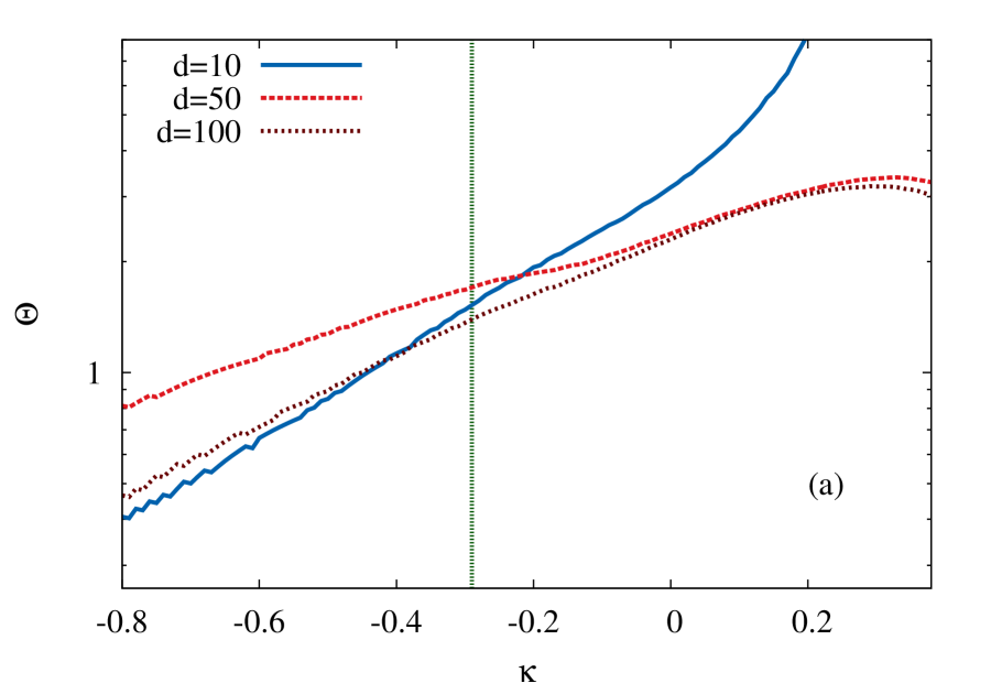
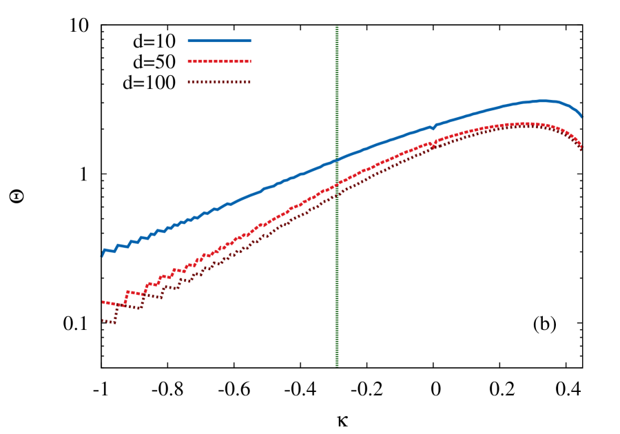
Analysis of the experiment of Miller et al. (2011).

In Figure 10 we reported the RMF model parameter combinations $(\kappa,c)$ required to explain the 9 beneficial second step mutations observed on the background of a highly fit first step mutation in the experiment of ?). Figure C1 displays the same data with the additive selection coefficient $c$ scaled by the standard deviation of the random fitness component, which in the case of the GPD distribution is given by

$$\sqrt{\mathrm{Var}(\eta)}=\sqrt{\frac{1}{(1-\kappa)^{2}(1-2\kappa)}}.$$ (C14)

LITERATURE CITED

- Aita (2008 Aita, T., 2008 Hierarchical distribution of ascending slopes, nearly neutral networks, highlands, and local optima at the dth order in an NK fitness landscape. J. Theor. Biol. 254: 252–263.
- Aita and Husimi (2000 Aita, T. and Y. Husimi, 2000 Adaptive walks by the fittest among finite random mutants on a Mt. Fuji-type fitness landscape II. Effect of small non-additivity. J. Math. Biol. 41: 207–231.
- Aita et al. (2000 Aita, T., H. Uchiyama, T. Inaoka, M. Nakajima, T. Kokubo, and Y. Husimi, 2000 Analysis of a local fitness landscape with a model of the rough Mt. Fuji-type landscape: application to prolyl endopeptidase and thermolysin. Biopolymers 54: 64–79.
- Bank et al. (2014 Bank, C., R.T. Hietpas, A. Wong, D.N. Bolon, and J.D. Jensen, 2014 A Bayesian MCMC approach to assess the complete distribution of fitness effects of new mutations: uncovering the potential for adaptive walks in challenging environments. Genetics 196: 841–852.
- Beisel et al. (2007 Beisel, C. J., D. R. Rokyta, H. A. Wichman, and P. Joyce, 2007 Testing the extreme value domain of attraction for distributions of beneficial fitness effects. Genetics 176: 2441–2449.
- Campos et al. (2002 Campos, P. R., C. Adami, and C. O. Wilke, 2002 Optimal adaptive performance and delocalization in NK fitness landscapes. Physica A 304: 495–506.
- Campos et al. (2003 Campos, P. R., C. Adami, and C. O. Wilke, 2003 Erratum to “Optimal adaptive performance and delocalization in NK fitness landscapes”. Physica A 318: 637.
- David and Nagaraja (2003 David, H. A. and H. N. Nagaraja, 2003 Order Statistics. Wiley-Interscience.
- de Haan and Ferreira (2006 de Haan, L. and A. Ferreira, 2006 Extreme Value Theory An Introduction. Springer.
- de Visser and Krug (2014 de Visser, J.A.G.M. and J. Krug, 2014 Empirical fitness landscapes and the predictability of evolution. Nat. Rev. Gen. 15: 480–490.
- Durrett and Limic (2003 Durrett, R. and V. Limic, 2003 Rigorous results for the NK model. Ann. Prob. 31: 1713–1753.
- Evans and Steinsaltz (2002 Evans, S. N. and D. Steinsaltz, 2002 Estimating some features of NK fitness landscapes. Ann. Appl. Prob. 12: 1299–1321.
- Flyvbjerg and Lautrup (1992 Flyvbjerg, H. and B. Lautrup, 1992 Evolution in a rugged fitness landscape. Physical Review A 46: 6714–6723.
- Foll et al. (2014 Foll, M., Y.-P. Poh, N. Renzette, A. Ferrer-Admitllal, C. Bank, A.-S. Malaspinas, G. Ewing, P. Liu, D. Wegmann, D.R. Caffrey, K.B. Zeldovich, D.N. Bolon, J.P. Wang, T.F. Kowalik, C.A. Schiffer, R.W. Finberg, and J.D. Jensen, 2014 Influenza Virus Drug Resistance: A Time-Sampled Population Genetics Perspective. PLoS Genetics 10: e1004185.
- Franke et al. (2011 Franke, J., A. Klözer, J. A. G. M. de Visser, and J. Krug, 2011 Evolutionary Accessibility of Mutational Pathways. PLoS Comput Biol 7: e1002134.
- Franke and Krug (2012 Franke, J. and J. Krug, 2012 Evolutionary accessibility in tunably rugged fitness landscapes. J. Stat. Phys. 148: 706–723.
- Franke et al. (2010 Franke, J., G. Wergen, and J. Krug, 2010 Records and sequences of records from random variables with a linear trend. J. Stat. Mech.: P10013.
- Gifford et al. (2011 Gifford, D. R., S. E. Schoustra, and R. Kassen, 2011 The length of adaptive walks is insensitive to starting fitness in Aspergillus nidulans. Evolution 65: 3070–3078.
- Gillespie (1983 Gillespie, J. H., 1983 A Simple Stochastic Gene Substitution Model. Theoretical Population Biology 23: 202–215.
- Gillespie (1984 Gillespie, J. H., 1984 Molecular evolution over the mutational landscape. Evolution 38 38: 1116–1129.
- Gillespie (1991 Gillespie, J. H., 1991 The Causes of Molecular Evolution. Oxford University Press.
- Graham et al. (1994 Graham, R. L., D. E. Knuth, and O. Patashnik, 1994 Concrete Mathematics (2 ed.). Addison-Wesley Publishing Company.
- Greene and Crona (2014 Greene, D. and K. Crona, 2014 The changing geometry of a fitness landscape along an adaptive walk. PLOS Computational Biology 10: e1003520.
- Gumbel and von Schelling (1950 Gumbel, E. J. and H. von Schelling, 1950 The Distribution of the Number of Exceedances. The Annals of Mathematical Statistics 21: 247–262.
- Hall et al. (2010 Hall, D. W., M. Agan, and S. C. Pope, 2010 Fitness epistasis among six biosynthetic loci the budding yeast Saccharomyces cerevisiae. J. Heredity 101: S75–S84.
- Hayashi et al. (2006 Hayashi, Y., T. Aita, H. Toyota, Y. Husimi, I. Urabe, and T. Yomo, 2006 Experimental Rugged Fitness Landscape in Protein Sequence Space. PLoS ONE 1: e96.
- Hegarty and Martinsson (2014 Hegarty, P. and A. Martinsson, 2014 On the existence of accessible paths in various models of fitness landscapes. Annals of Applied Probability (in press).
- Jain (2011 Jain, K., 2011 Number of adaptive steps to a local fitness peak. EPL 96: 58006.
- Jain and Krug (2007 Jain, K. and J. Krug, 2007 Deterministic and Stochastic Regimes of Asexual Evolution on Rugged Fitness Landscapes. Genetics 175: 1275–1288.
- Jain and Seetharaman (2011 Jain, K. and S. Seetharaman, 2011 Multiple adaptive substitutions during evolution in novel environments. Genetics 189: 1029–1043.
- Jain et al. (2011 Jain, K., J. Krug and S.C. Park, 2011 Evolutionary advantage of small populations on complex fitness landscapes. Evolution 65: 1945–1955.
- Joyce et al. (2008 Joyce, P., D. Rokyta, C. Beisel, and H. A. Orr, 2008 A General Extreme Value Theory Model for The Adaptation Of DNA Sequences under Strong Selection And Weak Mutation. Genetics 180: 1627–1643.
- Kassen and Bataillon (2006 Kassen, R. and T. Bataillon, 2006 Distribution of fitness effects among beneficial mutations prior to selection in experimental populations of bacteria. Nat. Genet. 38: 484–488.
- Kauffman and Levin (1987 Kauffman, S. and S. Levin, 1987 Towards a general theory of adaptive walks on rugged landscapes. J. Theor. Biol 128: 11–45.
- Kauffman (1993 Kauffman, S. A., 1993 The Origins of Order: Self-Organization and Selection in Evolution. Oxford University Press, USA.
- Kauffman and Weinberger (1989 Kauffman, S. A. and E. D. Weinberger, 1989 The NK model of rugged fitness landscapes and its application to maturation of the immune response. J. Theor. Biol. 141: 211–245.
- Kingman (1978 Kingman, J. F. C., 1978 A simple model for the balance between selection and mutation. J. Appl. Prob. 15: 1–12.
- Kryazhimskiy et al. (2009 Kryazhimskiy, S., G. Tkacik, and J. B. Plotkin, 2009 The dynamics of adaptation on correlated fitness landscapes. Proc. Nat. Acad. Sci. USA 106: 18638–18643.
- Limic and Pemantle (2004 Limic, V. and R. Pemantle, 2004 More rigorous results on the Kauffman-Levin model of evolution. Ann. Prob. 32: 2149–1287.
- Lobkovsky et al. (2011 Lobkovsky, A. E., Y. I. Wolf, and E. V. Koonin, 2011 Predictability of evolutionary trajectories in fitness landscapes. PLOS Computational Biology 7: e1002302.
- Lozovsky et al. (2009 Lozovsky, E. R., T. Chookajorn, K. M. Brown, M. Imwong, P. J. Shaw, S. Kamchonwongpaisan, D. E. Neafsey, D. M. Weinreich, and D. L. Hartl, 2009 Stepwise acquisition of pyrimethamine resistance in the malaria parasite. Proc. Nat. Acad. Sci. USA 106: 12025–12030.
- MacLean and Buckling (2009 MacLean, R. and A. Buckling, 2009 The distribution of fitness effects of beneficial mutations in Pseudomonas aeruginosa. PLoS Genetics 5: e1000406.
- Martin and Lenormand (2008 Martin, G. and T. Lenormand, 2008 The Distribution of Beneficial and Fixed Mutation Fitness Effects Close to an Optimum. Genetics 179: 907–916.
- Miller et al. (2011 Miller, C. R., P. Joyce, and H. A. Wichman, 2011 Mutational Effects and Population Dynamics During Viral Adaptation Challenge Current Models. Genetics 187: 185–202.
- Neidhart and Krug (2011 Neidhart, J. and J. Krug, 2011 Adaptive Walks and Extreme Value Theory. Physical Review Letters 107: 178102.
- Neidhart et al. (2013 Neidhart, J., I. G. Szendro, and J. Krug, 2013 Exact Results for Amplitude Spectra of Fitness Landscapes. J. Theor. Biol. 332: 218–227.
- Nowak and Krug (2013 Nowak, S. and J. Krug, 2013 Accessibility percolation on n-trees. EPL 101: 66004.
- Nowak et al. (2014 Nowak, S., J. Neidhart, I. G. Szendro, and J. Krug, 2013 Multidimensional epistasis and the transitory advantage of sex. Preprint arXiv:1403.6406.
- Ohta (1997 Ohta, T., 1997 Role of Random Genetic Drift in the Evolution of Interactive Systems. J. Mol. Evol. 44: S9–S14.
- Orr (2002a Orr, H. A., 2002a A Minimum on the Mean Number of Steps Taken in Adaptive Walks. J. theor. Biol. 220: 241–247.
- Orr (2002b Orr, H. A., 2002b The population genetics of adaptation: the adaptation of DNA sequences. Evolution 56(7): 1317–1330.
- Orr (2003 Orr, H. A., 2003 The distribution of fitness effects among beneficial mutations. Genetics 163: 15–1526.
- Orr (2005a Orr, H. A., 2005a The genetic theory of adaptation: a brief history. Nat. Rev. Gen. 6: 119–127.
- Orr (2005b Orr, H. A., 2005b Theories of adaptation: what they do and don’t say. Genetica 123: 3–13.
- Orr (2006a Orr, H. A., 2006a The Population Genetics of Adaptation on Correlated Fitness Landscapes: The Block Model. Evolution 60: 1113–1124.
- Orr (2006b Orr, H. A., 2006b The distribution of fitness effects among beneficial mutations in Fisher’s geometric model of adaptation J. Theor. Biol. 238: 279–285.
- Orr (2010 Orr, H. A., 2010 The population genetics of beneficial mutations. Phil. Trans. R. Soc. B . 365: 1195–1201.
- Østman et al. (2012 Østman, B., A. Hintze, and C. Adami, 2012 Impact of epistasis and pleiotropy on evolutionary adaptation. Proc. Roy. Soc. B 279: 247–256.
- Park et al. (2014 Park, S. C., I. G. Szendro, J. Neidhart, and J. Krug, 2014 Phase transition in adaptive walks on the rough Mount Fuji fitness landscape. Manuscript in preparation.
- Perelson and Macken (1995 Perelson, A. S. and C. A. Macken, 1995 Protein evolution on partially correlated landscapes. Proc. Natl. Acad. Sci. USA 92: 9657–9661.
- Pickands (1975 Pickands, J., 1975 Statistical inference using extreme order statistics. Annals of Statistics 3: 119–131.
- Roberts and Zhao (2013 Roberts, M. I. and L. Z. Zhao, 2013 Increasing paths in regular trees. Electron. Commun. Probab. 18: 1–10.
- Rokyta et al. (2005 Rokyta, D., P. Joyce, S. Caudle, and H. Wichman, 2005 An empirical test of the mutational landscape model of adaptation using a single-stranded DNA virus. Nat. Genet. 37: 441–444.
- Rokyta et al. (2006 Rokyta, D. R., C. J. Beisel, and P. Joyce, 2006 Properties of adaptive walks on uncorrelated landscapes under strong selection and weak mutation. Journal of Theoretical Biology 243: 114–120.
- Rokyta et al. (2008 Rokyta, D. R., C. J. Beisel, P. Joyce, M. T. Ferris, C. L. Burch, and H. A. Wichman, 2008 Beneficial Fitness Effects Are Not Exponential for Two Viruses. J. Mol. Evol. 67: 368–376.
- Rowe et al. (2010 Rowe, W., M. Platt, D. C. Wedge, P. J. Day, D. B. Kell, and J. Knowles, 2010 Analysis of a complete DNA-protein affinity landscape. J. R. Soc. Interface 7: 397–408.
- Schenk et al. (2012 Schenk, M., I. Szendro, J. Krug, and J. de Visser, 2012 Quantifying the Adaptive Potential of an Antibiotic Resistance Enzyme. PLoS Genetics 8. e1002783.
- Schenk et al. (2013 Schenk, M. F., I. G. Szendro, M. L. M. Salverda, J. Krug, and J. A. G. M. de Visser, 2013 Patterns of epistasis between beneficial mutations in an antibiotic resistance gene. Molecular Biology and Evolution 30: 1779–1787.
- Schmiegelt and Krug (2014 Schmiegelt, B. and J. Krug, 2014 Evolutionary accessibility of modular fitness landscapes. J. Stat. Phys. 154: 334–355.
- Schoustra et al. (2012 Schoustra, S. E., T. Bataillon, D. R. Gifford, and R. Kassen, 2012 The Properties of Adaptive Walks in Evolving Populations of Fungus. PLoS Biology 7: e1000250.
- Seetharaman and Jain (2014 Seetharaman, S. and K. Jain, 2014 Adaptive walks and distribution of beneficial fitness effects. Evolution 68: 965–975.
- Smid and Stam (1975 Smid, B. and A.J. Stam, 1975 Convergence in distribution of quotients of order statistics. Stoch. Proc. Appl. 3: 287–292.
- Sniegowski and Gerrish (2010 Sniegowski, P. D. and P. J. Gerrish, 2010 Beneficial mutations and the dynamics of adaptation in asexual populations. Phil. Trans. R. Soc. B 365: 1255–1263.
- Stadler and Happel (1999 Stadler, P. F. and R. Happel, 1999 Random field models for fitness landscapes. J. Math. Biol. 38: 435–478.
- Szendro, Franke et al. (2013 Szendro, I. G., J. Franke, J. A. G. M. de Visser, and J. Krug, 2013 Predictability of evolution depends nonmonotonically on population size. Proceedings of the National Academy of Sciences USA 110: 571–576.
- Szendro, Schenk et al. (2013 Szendro, I. G., M. F. Schenk, J. Franke, J. Krug, and J. A. G. M. de Visser, 2013 Quantitative analyses of empirical fitness landscapes. J. Stat. Mech.: Theor. Exp.: P01005.
- Weinberger (1990 Weinberger, E., 1990 Correlated and uncorrelated fitness landscapes and how to tell the difference. Biol. Cybern. 63: 325–336.
- Weinreich et al. (2006 Weinreich, D., N. Delaney, M. DePristo, and D. Hartl, 2006 Darwinian evolution can follow only very few mutational paths to fitter proteins. Science 312: 111–114.
- Weinreich et al. (2013 Weinreich, D. M., Y. Lan, C. S. Wylie, and R. B. Heckendorn, 2013 Should evolutionary geneticists worry about higher-order epistasis? Current Opinion in Genetics and Development 23: 700–707.
- Welch and Waxman (2005 Welch, J. J. and D. Waxman, 2005 The nk model and population genetics. J. Theor. Biol. 234: 329–340.
- Wergen et al. (2011 Wergen, G., J. Franke, and J. Krug, 2011 Correlations Between Record Events in Sequences of Random Variables with a Linear Trend. J. Stat. Phys. 144: 1206–1222.