11email: jmaiz@iaa.es 22institutetext: UK Astronomy Technology Centre, Royal Observatory Edinburgh, Blackford Hill, Edinburgh, EH9 3HJ, UK
33institutetext: Departamento de Física, Universidad de La Serena, Av. Cisternas 1200 Norte, La Serena, Chile
44institutetext: Armagh Observatory, College Hill, Armagh BT61 9DG, UK
55institutetext: Department of Physics & Astronomy, Hounsfield Road, University of Sheffield, S3 7RH, UK
66institutetext: Centro de Astrobiología, CSIC-INTA, Ctra. Torrejón a Ajalvir km 4, E-28 850 Torrejón de Ardoz, Madrid, Spain
77institutetext: Instituto de Astrofísica de Canarias, E-38 200 La Laguna, Tenerife, Spain
88institutetext: Departamento de Astrofísica, Universidad de La Laguna, E-38 205 La Laguna, Tenerife, Spain
99institutetext: Space Telescope Science Institute, 3700 San Martin Drive, Baltimore, MD 21 218, USA
1010institutetext: Institute for the Environment, Physical Sciences and Applied Mathematics, Keele University, ST5 5BG, UK
The VLT-FLAMES Tarantula Survey
Abstract
Context. The commonly used extinction laws of Cardelli et al. (1989) have limitations that, among other issues, hamper the determination of the effective temperatures of O and early B stars from optical and NIR photometry.
Aims. We aim to develop a new family of extinction laws for 30 Doradus, check their general applicability within that region and elsewhere, and apply them to test the feasibility of using optical and NIR photometry to determine the effective temperature of OB stars.
Methods. We use spectroscopy and NIR photometry from the VLT-FLAMES Tarantula Survey and optical photometry from HST/WFC3 of 30 Doradus and we analyze them with the software code CHORIZOS using different assumptions, such as the family of extinction laws.
Results. We derive a new family of optical and NIR extinction laws for 30 Doradus and confirm its applicability to extinguished Galactic O-type systems. We conclude that by using the new extinction laws it is possible to measure the effective temperatures of OB stars with moderate uncertainties and only a small bias, at least up to mag.
Key Words.:
Open clusters and associations: individual: 30 Doradus — Dust, extinction — Magellanic Clouds — Stars: fundamental parameters — Stars: early-type1 Introduction
Astronomy is entering a time when massive photometric surveys allow us to obtain information about a very large number of objects. Projects such as Gaia and the Large Synoptic Survey Telescope (LSST) will reinforce this trend in the next decade. The main goal of these surveys is to measure the intrinsic properties of these objects, such as the effective temperature, luminosity, and metallicity of stars; the mass, age, and metallicity of stellar clusters; or the redshift and type of galaxies. These surveys include not only large numbers of targets, but also detailed calibration mechanisms that lead to (internal) precisions and (external) accuracies at the level of one hundredth of a magnitude. In other words, we have not only data in large quantities but also with high quality in the form of random and systematic errors that are significantly lower than what was typical twenty years ago. This high photometric quality is also extended to space missions such as the Hubble Space Telescope (HST) and is due to the stability of the space environment and the resources devoted to ensure the uniformity of the data.
Despite such high quality, there is (and always will be) one obstacle for the derivation of the intrinsic properties of astronomical objects: extinction. Every observation has to be corrected for the presence of dust between the target and the observer and that can be (and in many cases is) the main limitation. In the 1980s the great success of the International Ultraviolet Explorer (IUE) satellite prompted a revived interest in the subject of extinction that culminated with the groundbreaking work of Cardelli et al. (1989, hereafter CCM). that paper provided for the first time a family of extinction laws that extended from the IR to the UV while simultaneously characterizing the type of extinction with a single parameter, (see Maíz Apellániz 2013a for a discussion on the name and the precise nature of the parameter). These two characteristics made the CCM laws a resounding success and the paper one of the most cited in astronomy in the last quarter of a century.
Despite their unquestioned relevance, different studies in the last two decades have revealed several issues with some aspects of the CCM laws:
-
•
the use of band-integrated [ and ] quantities to define the amount and type of extinction instead of their monochromatic equivalents ( and , respectively)111It cannot be emphasized enough that using to parameterize an extinction law is a serious mistake. depends not only on the extinction law but also on the amount of extinction and the input SED. The reader is referred to Figure 3 of Maíz Apellániz (2013a) to quantify the effect. The parameter called in CCM is not really that (in the sense that an extinction law with a given value of that parameter does not yield that value of for an arbitrary amount of extinction and an arbitrary SED), but a monochromatic value. In addition, this type of effect in broad-band photometry has been known at least since Blanco (1957) but appears to be overlooked by a significant fraction of the astronomical community.;
-
•
the validity of a fixed extinction law in the NIR;
-
•
the functional form used in the optical;
-
•
the reality of the correlation between and UV extinction;
-
•
the applicability of the laws beyond the and values of the sample used to derive them;
-
•
the photometric calibration of the filters.
These issues are discussed in Maíz Apellániz (2013a), where the reader is referred for details, and they are the reasons that prompted us to attempt an improvement of the CCM laws, concentrating on the correction for extinction for photometric data, their most commonly used application.
This paper is part of a series on the VLT-FLAMES Tarantula Survey. The reader is referred to the first paper, Evans et al. (2011), for details on the project. Within the series, this paper on the optical and NIR extinction law in 30 Doradus and its application to the determination of effective temperatures () is part of a subseries on extinction and the ISM. The subseries started with the work of van Loon et al. (2013) on diffuse interstellar bands and neutral sodium and will continue with another paper on the spatial distribution of extinction in 30 Doradus (Maíz Apellániz et al. in preparation).
We start by describing the spectroscopic and photometric data in this paper. We then perform different experiments with the data by processing them with CHORIZOS (Maíz Apellániz, 2004). The results are discussed and possible future work is described. The paper ends with three appendixes on (a) the detailed changes introduced by the new laws, (b) CHORIZOS and the spectral energy distributions (SEDs) used for this paper, and (c) the extinction along a sightline with more than one type of dust.
2 Data
2.1 Spectral types and effective temperatures
Our sample was selected mostly from the VFTS O-star sample (Walborn et al., 2014) with the addition of some O and B stars also observed with VFTS. The majority of the targets were observed by VFTS using the Medusa–Giraffe mode of the Fibre Large Array Multi-Element Spectrograph (FLAMES) instrument (Pasquini et al., 2002). Each star was observed with the LR02 and LR03 settings of the Giraffe spectrograph, which provided coverage of 3960-5071 Å (at of 7000 to 8500). Some of the stars in the R136 region (identifiable by their VFTS numbers above 1000), the massive cluster at its core, were observed with the LR02 setting using the ARGUS–Giraffe mode222These stars are not included in Walborn et al. (2014). Neither are the B stars in this paper., which gives a comparable wavelength coverage but at a greater resolving power (). Comprehensive classifications of these data for the O-type stars were presented by Walborn et al. (2014), which also took into account binary companions detected by multi-epoch observations with the LR02+LR03 settings (see Sana et al. 2013). The B stars were classified for this paper333A future VFTS B-star classification paper will appear as Evans et al., we have verified that there is a good agreement between the independently derived spectral classifications for the two works..
The O-type stars in this paper sample the region of the 30 Doradus nebula imaged by the HST/WFC3 data described below, except for the very central part of R136 due to its dense stellar crowding. In the original target selection the only strong restriction was a faint-magnitude cut ( 17 mag) to ensure sufficient signal-to-noise in the spectra of each target. The lack of color cuts should ensure that (moderately) reddened O-type stars were included, i.e., we are not strongly biased toward sightlines with low extinction. The O-type census obtained by VFTS is moderately complete across a 20′ field (excluding the central 033). For instance, in the course of their analysis of the feedback from hot, luminous stars in 30 Dor (which also includes early B-type objects), Doran et al. (2013) estimated that the Medusa VFTS observations were 76% complete.
The spectral types were transformed into effective temperatures () using the calibration of Martins et al. (2005) shifted upwards by 1000 K to account for the metallicity difference between the Milky Way and the LMC (Mokiem et al., 2007; Doran et al., 2013). The shift is consistent with an ongoing analysis in the VFTS collaboration using FASTWIND grids (see Sabín-Sanjulián et al. 2013 for some first results) and the IACOB-Grid Based Automatic Tool (IACOB-GBAT, Simón-Díaz et al. 2011). From now on, the derived from the spectral types will be called spectroscopic temperatures.
As described in Appendix B, LMC-metallicity TLUSTY models are used as the intrinsic (extinction-free) SEDs for a given spectroscopic temperature. Since TLUSTY does not include wind effects, we should check for possible biases in the intrinsic colors. For a subsample of 12 stars analyzed individually within the VFTS collaboration with CMFGEN models (which include wind effects, see Bestenlehner et al. in preparation), we have compared the TLUSTY and the CMFGEN SEDs to check for possible systematic intrinsic color differences and we have found that they are very small ( mag) when comparing models of the same . Some slightly larger ( mag) color variations were found in individual fits but these can be ascribed to differences on the order of 1000-2000 K between our spectroscopic temperatures (derived from the spectral types) and the star-by-star values of derived from the CMFGEN analysis. Such variations are random, not systematic, and expected given the natural range of existent within a given spectral type. Therefore, the use of values of derived from spectral types and TLUSTY SEDs (as opposed to the more costly alternative of deriving individual SEDs for all the stars in the sample with, e.g. CMFGEN) may introduce a small amount of noise but no biases.
2.2 NIR photometry
Object (K) VFTS 385 42 900 0.3130.010 4.300.20 VFTS 410 36 900 0.4920.027 5.150.50 VFTS 422 43 400 0.5110.010 4.860.13 VFTS 432 34 900 0.4890.010 4.520.15 VFTS 436 36 900 0.2960.011 4.650.32 VFTS 440 38 500 0.3200.010 4.570.20 VFTS 451 37 900 0.5860.017 6.440.36 VFTS 460 36 900 0.6770.010 3.970.09 VFTS 464 32 300 0.6460.031 6.720.46 VFTS 465 41 900 0.7400.009 5.270.09 VFTS 472 39 900 0.5340.010 3.720.12 VFTS 484 38 900 0.3860.010 5.090.18 VFTS 491 39 900 0.5630.010 3.950.11 VFTS 493 33 900 0.6360.010 4.000.11 VFTS 494 35 900 0.6120.010 3.970.11 VFTS 498 32 300 0.4410.011 5.030.27 VFTS 505 32 300 0.3230.017 3.940.41 VFTS 506 47 700 0.3240.010 4.250.18 VFTS 508 32 300 0.4380.011 4.260.17 VFTS 511 41 900 0.4020.010 4.160.17 VFTS 512 47 700 0.4580.010 4.410.13 VFTS 518 44 300 0.5290.010 4.000.12 VFTS 520 26 400 0.3790.010 3.180.21 VFTS 521 33 900 0.3660.012 4.840.35 VFTS 525 26 000 0.3250.010 4.810.20 VFTS 532 45 900 0.4550.010 4.130.14 VFTS 543 33 300 0.3290.011 3.170.22 VFTS 559 31 100 0.3670.011 4.720.28 VFTS 560 32 300 0.3280.010 4.550.24 VFTS 561 33 900 0.3760.010 4.170.20 VFTS 563 30 100 0.4040.010 4.020.16 VFTS 565 32 300 0.2980.011 4.670.33 VFTS 566 45 500 0.2850.010 5.260.26 VFTS 575 25 000 0.2570.010 3.140.29 VFTS 577 39 900 0.5550.010 4.600.14 VFTS 579 33 900 0.3760.034 6.330.83 VFTS 585 37 900 0.3150.010 4.540.19 VFTS 587 31 100 0.2790.010 4.430.28 VFTS 591 25 000 0.4220.010 4.440.14 VFTS 596 36 900 0.3960.010 4.060.16 VFTS 597 34 900 0.3100.010 3.990.21
Object (K) VFTS 598 29 100 0.5410.010 3.690.16 VFTS 599 45 500 0.3400.010 4.510.18 VFTS 601 40 900 0.3740.010 4.270.17 VFTS 607 30 100 0.2970.010 5.040.31 VFTS 608 43 400 0.4250.010 4.330.15 VFTS 609 33 300 0.3710.012 4.150.39 VFTS 611 35 900 0.3840.010 3.680.18 VFTS 612 26 400 0.4130.010 4.060.17 VFTS 616 27 300 0.3600.010 4.090.18 VFTS 619 36 900 0.3720.010 4.280.18 VFTS 635 31 700 0.3120.010 3.590.20 VFTS 637 26 400 0.2920.010 3.090.25 VFTS 646 28 000 0.3590.010 4.340.17 VFTS 647 35 900 0.3390.012 4.620.50 VFTS 648 40 500 0.3110.010 4.340.19 VFTS 649 32 300 0.3270.010 3.930.20 VFTS 651 37 900 0.3460.010 4.020.17 VFTS 654 33 900 0.3050.010 4.900.24 VFTS 656 36 000 0.2900.010 4.370.22 VFTS 660 32 300 0.2800.010 4.990.27 VFTS 664 36 500 0.3990.010 4.190.15 VFTS 667 39 900 0.3410.010 3.990.18 VFTS 676 26 400 0.2970.012 5.500.56 VFTS 681 26 400 0.2860.010 3.800.24 VFTS 686 25 000 0.3830.010 4.170.16 VFTS 688 30 100 0.3750.010 3.650.16 VFTS 692 28 600 0.2260.011 6.110.45 VFTS 702 35 900 0.5830.011 4.300.17 VFTS 705 26 400 0.3230.010 3.950.20 VFTS 706 38 900 0.4310.010 3.540.13 VFTS 707 27 300 0.3330.010 3.840.19 VFTS 710 31 700 0.2870.010 3.160.22 VFTS 712 26 400 0.4560.012 3.460.14 VFTS 717 33 300 0.4660.010 4.000.14 VFTS 728 29 000 0.3090.010 3.900.21 VFTS 1002 31 700 0.3540.012 4.630.50 VFTS 1006 38 500 0.5230.012 3.520.18 VFTS 1007 38 500 0.4080.011 4.580.25 VFTS 1018 41 300 0.4440.010 4.750.15 VFTS 1020 44 900 0.4040.010 4.650.19 VFTS 1028 43 600 0.2980.011 5.330.31 VFTS 1035 33 900 0.2790.011 4.560.38
Near-IR photometry for the vast majority of the VFTS targets is available from the Magellanic Clouds survey by Kato et al. (2007) using the InfraRed Survey Facility (IRSF) 1.4 m telescope in South Africa. The IRSF () magnitudes and their associated errors used in our analysis were presented in Table 6 in Evans et al. (2011). The IRSF photometry was converted into the 2MASS system (Skrutskie et al., 2006) by selecting a number of isolated stars with good S/N in both catalogs in the 30 Doradus region and deriving the corresponding linear transformations. We obtain the following relationships:
| (1) |
| (2) |
| (3) |
In order to ensure the accuracy of the NIR photometry, we compared the values with those of the VISTA VMC survey (Cioni et al., 2011; Rubele et al., 2012) and, for fields with strong nebulosity, with the ground-based photometry of Rubio et al. (1998) and the HST photometry of Walborn et al. (1999). In cases with significant discrepancies we adjusted the values and increased the uncertainties of the used photometry.
2.3 Optical photometry
The optical photometry used in this paper was obtained with the UVIS channel of the Wide Field Camera 3 aboard HST as part of its Early Release Science program. Five filters were used: F336W (), F438W (), F555W (), F656N (H), and F814W (), see De Marchi et al. (2011) for details. Particular care was taken during the preparation of the observations to include a wide range of exposure times in each filter; if that had not been done, the bright stars in the central region of 30 Doradus (many of them included in the sample of this paper) would have been saturated. The multiple WFC3 frames were combined into a single image per filter using Multidrizzle444http://stsdas.stsci.edu/multidrizzle/ . after manually measuring the individual shifts and carefully selecting for each output pixel the information from the frames with the best S/N that were free of defects and not saturated.
In principle, one can use PSF fitting to obtain the photometry of HST images. However, there are two reasons that advise against it in our case. (a) We need to combine the optical HST photometry with the ground-based NIR photometry: what appears as a single source in the latter may be (and in a number of cases is) multiple. (b) In some regions of 30 Doradus the background is highly variable and a straightforward PSF fitting may underestimate the uncertainties associated with its subtraction. Hence, we decided to do source-by-source aperture photometry in which we considered:
-
•
The number of point sources within the equivalent ground-based aperture. For isolated sources we used a single, small aperture. For multiple sources, we increased the aperture and applied an aperture correction or used multiple apertures (but see below for the final selection).
-
•
Background subtraction. We considered a worst-case scenario in which the variations in the nearby background were taken as systematic instead of random. That is, the value and the dispersion of the background were measured and the effect of the dispersion was added as an additional source of uncertainty by allowing the background to move up and down systematically (and not randomly on each pixel of the aperture).
Considering all the uncertainty sources, a threshold of 0.02 magnitudes was determined to be needed for the uncertainty of all of the measured WFC3 magnitudes. We obtained the photometry for the five filters but we excluded F656N from the fit (since some O stars have H filled or even in emission).
2.4 Final sample selection
Our initial sample consisted of 141 stars observed in the WFC3-ERS program. We analyzed each case individually and we eliminated those cases where [a] multiplicity was likely to yield a heterogeneous SED, [b] the photometry was internally or externally inconsistent (this could be caused by instrumental effects, e.g. undetected cosmic rays, or physical reasons, e.g. the system is photometrically variable), [c] the spectral type was of poor quality, or [d] the spectroscopic was lower than 24 000 K (in these cases the differences in magnitude in the Balmer jump between adjacent spectral types become too large for our purposes). After the elimination process, we were left with 83 stars (67 O stars and 16 B stars). They are listed in Table 1.
3 Experiments
The experiments in this paper are performed with v3.2 of the bayesian code CHORIZOS (Maíz Apellániz, 2004). The procedure consists of fitting the available -like photometry to a family of synthetic SED models allowing for different parameters to be left free or kept fixed and for different extinction laws to be used. This method allows the amount and type of extinction (along with possibly other quantities such as or luminosity class) to be simultaneously fitted. See example 2 in Maíz Apellániz (2004) and Maíz Apellániz et al. (2007). The method has been called “extinction without standards” by Fitzpatrick & Massa (2005). See Appendix B and Maíz Apellániz (2013b) for information on the used LMC-metallicity SED grid.
3.1 Experiment 1: CCM laws and fixed


For our first experiment, we:
-
•
Fix the metallicity (Lanz & Hubeny, 2003) and distance ( pc) to the LMC values.
-
•
Fix the for each star to the value determined from its spectral type (see above).
-
•
Use the CCM family of extinction laws.
-
•
Leave three free parameters: (photometric) luminosity class (see Appendix B), type of extinction [], and amount of extinction [].
-
•
Since for each star we have magnitudes and free parameters, the solution has 4 degrees of freedom.
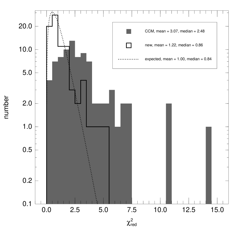
Running CHORIZOS under these conditions yields results for and with relatively good precision (small uncertainties) but the accuracy of the fit is unsatisfactory due to the poor results of the distribution (filled histogram in Figure 1). The distribution has a mean of 3.07 and a median of 2.48 and its overall appearance is different from the expected distribution (shown as a dotted line, mean of 1.00 and median of 0.84). The main peak is shifted towards the right and a significant tail is seen to have . This is a first sign that there is something wrong with either the photometric data, the range of parameters, the input SEDs, or the extinction laws. In order to find the cause we have to analyze the results in more detail.
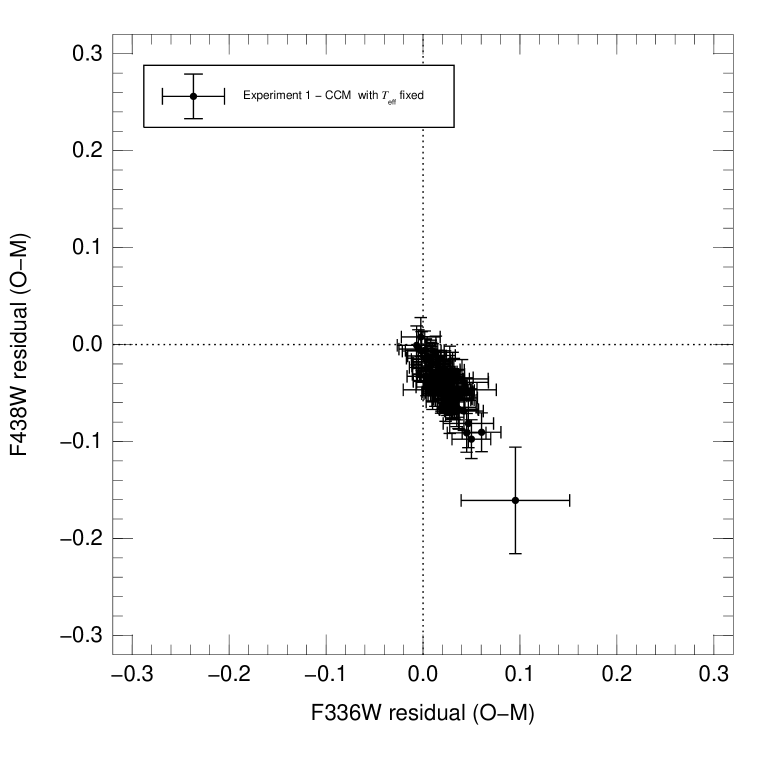
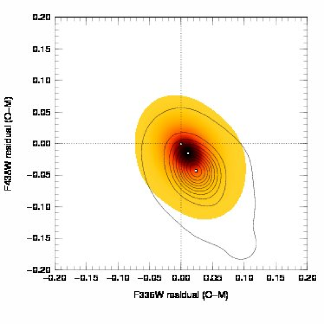
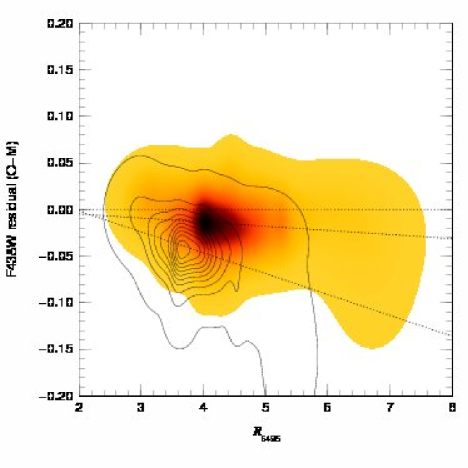
Figure 2 shows some fit residuals (observed minus model) plotted against one another and against and . Several effects are seen:


-
•
The F336W () and F438W () residuals are strongly anticorrelated and these filters carry a good fraction of the weight of in the targets where is high. CHORIZOS is finding as the best possible solution an intermediate SED that is too bright in and too dim in but cannot find an optimal solution because it is not within the allowable ones. At a lower level, similar anticorrelations are found between other residuals from adjacent filters.
-
•
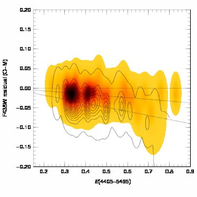
The F438W residual is correlated with the amount of extinction. This points towards the extinction law as the culprit, since for low values of the extinction the residuals show only a small bias in their distribution.
-
•
The F438W is also clearly correlated with . For , the residual distribution is centered around zero but for high values there is a clear offset. This indicates that the CCM laws for the lower values of provide a better fit than for higher values.
Therefore, these results lead us to think that the problem is in the exact form of the CCM extinction laws, a hypothesis that we will test in subsequent experiments. If the CCM family of extinction laws does not provide an adequate solution, one should first test an existing alternative. Fitzpatrick (1999) presented a family of -dependent extinction laws (from now on, we will call them F99 laws) which we have also implemented in CHORIZOS. Executing experiment 1 with these alternate laws we find that they do not provide an adequate solution, either. The distribution has a mean of 4.43 and a median of 3.95, i.e. even worse than the CCM result.
3.2 Experiment 2: CCM laws and variable
Before attempting a modification of the CCM family of extinction laws, we perform a second experiment with them and an important modification on the conditions: we leave as a free parameter. This increases to 4 and leaves just 3 degrees of freedom. It also introduces a new measure of the accuracy of the fit: how do the calculated (photometric) compare with their spectroscopic counterparts.
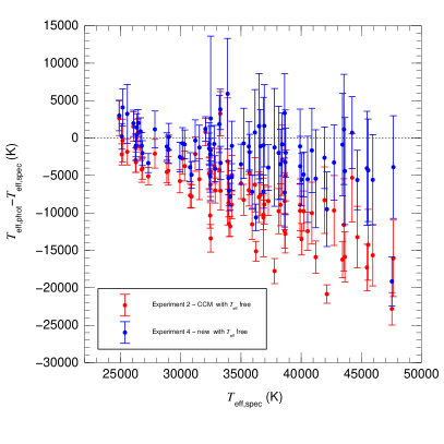
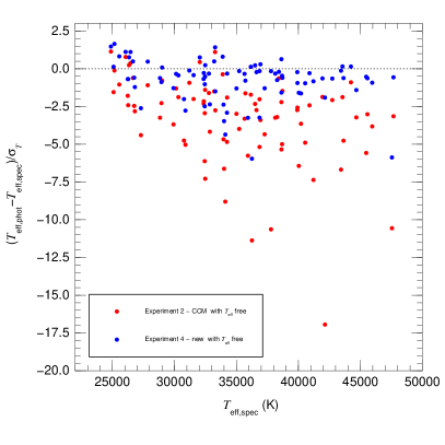
The results of the second experiment look encouraging at first. They yield a distribution with a mean of 1.09 and a median of 0.91, which are very similar to the results expected for an ideal experiment with 3 degrees of freedom (1.00 and 0.78, respectively). The problem arises from the differences between the photometric and spectroscopic . The photometric values are lower by an average of 7700 K and there is a significant trend that makes the results get worse for higher values of (Figure 3). Looking at the results in a different way, the spectroscopic temperature range of 30 000-40 000 K is approximately mapped into a 25 000-30 000 K range in photometric temperature (shifted downwards but also compressed). When normalized by their (CHORIZOS-derived photometric) uncertainties, the difference between the two values has a mean of and a standard deviation of , a long way from the expected respective values of and in an ideal experiment. Note that the intrinsic scatter in within a given spectral type and luminosity class is 1000-2000 K, much lower than the offset detected here.
This second experiment allows us to draw two important conclusions:
-
•
CCM laws cannot be used to accurately derive the of O stars from photometry because they introduce a significant bias even for moderate values of (most of the stars in our sample are in the range between 0.3 and 0.7 mag).
-
•
The main difference in the photometry of e.g. a 30 000 K and a 40 000 K star of similar gravities lies in the -like color because in the optical and NIR their SEDs are relatively well described by the Rayleigh-Jeans law, with the main difference arising from the Balmer jump555Note that the WFC3 F336W-F438W color provides a cleaner measurement of the Balmer jump than Johnson’s , see Maíz Apellániz (2005, 2006, 2007).. Therefore, the fact that experiment 2 yields a good distribution but with the wrong temperatures is telling us that the problem of the CCM laws is in the same wavelength region (3000-5000 Å), since it should be possible to tweak the laws in that region to counteract the artificial temperature shift by an equivalent change in the -like colors. More specifically, the results of experiments 1 and 2 indicate that the problem with the CCM laws appears to be concentrated in the band for high values of .
3.3 Experiment 3: New laws and fixed


The two previous experiments allowed us to qualitatively determine in which direction we should introduce corrections to the CCM laws in order to provide a better fit to the observed photometry (making the distribution look more similar to the expected distribution in the first case and yielding better temperature estimates in the second). The ideal way to quantitatively derive these corrections would be to obtain good-quality spectrophotometry with a large wavelength coverage (i.e. the same method Whitford 1958 used) but, unfortunately, that is not available for an appropriate sample. We have to resort to an iterative process in which we estimate a new family of laws (using the qualitative criteria above) and proceed by trial and error running CHORIZOS with the estimate, analyzing the behavior of the photometric residuals in the experiment 1 equivalent (from now on, experiment 3) and the temperature differences in the experiment 2 equivalent (from now on, experiment 4) to improve on the results. After more than 20 iterations (each one taking several days), we arrived at the new family. Details of the procedure are given in Appendix A.
The improvements introduced by the final form of the new laws can be seen in the first place in Figure 1, which compares the results of experiments 1 and 3. The new laws yield a distribution with a mean of 1.22 and a median of 0.86. The second value is very similar to the ideal result of 0.84 while the first one is only slightly higher than the perfect result of 1.00. Most of the difference can be attributed to the existence of four stars with between 3.5 and 5.5. Additional improvements in experiment 3 with respect to experiment 1 can be seen in Figure 4. In the top panel, the anticorrelation between F336W and F438W has diminished considerably and the outliers have disappeared. In the bottom two panels we see that the F438W residuals now have a weaker dependence on and , respectively. In summary, the new laws provide a significantly better fit to the observed photometry if spectroscopic temperatures are used as an input to constrain the unextinguished SED.
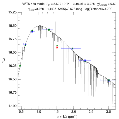
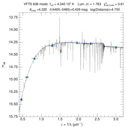
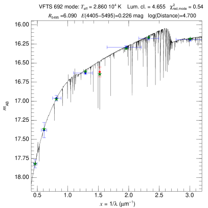
Four examples of results from experiment 3 are shown in Figure 5. Note the small extent of the vertical error bars (photometric uncertainties) and the good agreement between them and the synthetic photometry (green stars). Figure 6 shows the relationship between the , , and results for experiments 1 and 3 (see also Table 1). In experiment 3 the results for are consistently lower and the results for consistently higher than those in experiment 1. Note, however, that the results for remain almost unchanged. A linear regression yields , so that for e.g. mag, is typically mag. Note, also, that in many cases the relative errors in are smaller than those expected from the relative errors in and because these two quantities are usually anticorrelated in the likelihood CHORIZOS outputs.
3.4 Experiment 4: New laws and variable
As previously mentioned, our fourth experiment is the equivalent to the second one with the new laws. The comparison between the photometric temperatures derived from experiments 2 and 4 is shown in Figure 7. From the graphical comparison it is clear that the results from the fourth experiment are a significant improvement. Indeed, the mean difference between the photometric and spectroscopic temperatures has a mean of 2200 K (less than 1/3 of the previous difference) and the normalized difference distribution now has a mean of and a standard deviation of (compare to the ideal results of and ). These results, though not perfect, are actually quite good. After all, typical spectroscopic determinations of for O stars have uncertainties of 1000-2000 K. The results here have typical random uncertainties of 2000 K for = 30 000 K and 6000 K for = 45 000 K. Hence, we can claim that it is possible to photometrically measure the effective temperature of an O star with [a] good accuracy (systematic biases comparable to random uncertainties, lower in most cases) and [b] good precision (random uncertainties only a factor of two higher than what is currently possible with spectroscopy). Spectroscopy provides better results by a factor of two and adds additional information on e.g. luminosity, metallicity, or ; so it is still preferred for detailed studies of individual objects. However, under the right conditions photometry yields acceptable measurements for O stars (and even better ones for B stars, whose Balmer jump is more sensitive to temperature) with the advantage of its efficiency in terms of number of objects observed per unit of time.
We have covered a long distance since Hummer et al. (1988), who entitled their paper “Failure of continuum methods for determining the effective temperature of hot stars” and who started their abstract by stating: “We demonstrate that for hot stars ( K) methods based on the integrated continuum flux are completely unreliable discriminators of the effective temperature”. Improvements on data, models, and techniques helped to fix the issues that plagued these authors. As suspected by Maíz Apellániz & Sota (2008), the last required step was an accurate extinction law.
4 Discussion
4.1 How good are the new laws?
In a nutshell, better than CCM but not perfect. A perfect extinction law should show symmetrical residuals with respect to zero in Figure 4 and also show a symmetrical distribution with respect to zero in the vertical axis of Figure 7. In principle, these issues could also be attributed to an incorrect spectral type- scale or to problems in the TLUSTY SEDs (more on that later), but given the large discrepancies observed in the first two experiments, it is more likely than an improvement in the extinction law could reduce the discrepancies even further. As stated elsewhere in this paper, the final word on optical and NIR extinction laws will have to be provided by spectrophotometric analyses. A preliminary and limited study along that line is presented in the next two subsections.
We should also ask ourselves why is it that the new laws are better than the CCM ones in the optical and NIR. The answer is threefold: better photometry, better technique, and better sample. WFC3 photometry is better calibrated than Johnson’s (Maíz Apellániz, 2006) and 2MASS has also allowed an all-sky calibration in the NIR. Spline interpolation is a more appropriate technique than using a seventh-degree polynomial. But the largest difference is in the sample. CCM used only 29 stars, some with spectral types that have been updated since then, and their sample is heavily biased towards . Indeed, CCM had only one star with both and mag, and that star (Herschel 36) turns out to have a NIR excess (Arias et al., 2006), to be a high-order multiple system (Arias et al., 2010), and to have its IUE spectra highly contaminated by the nearby Hourglass acting as a reflection nebula (Maíz Apellániz et al. in preparation): its use to derive an extinction law has to be considered very carefully, especially if it is the only representative of a category. On the other hand, the sample in the new laws is almost three times larger and, more importantly, it covers the range better (with the exception of ).
4.2 30 Doradus stars with STIS spectrophotometry
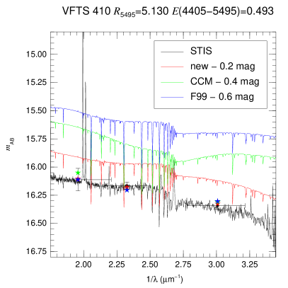
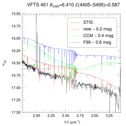
Obtaining optical spectrophotometry of stars in 30 Doradus from the ground is difficult due to [a] crowding (which introduces additional stars in a wide slit) and [b] strong nebular contamination (which easily saturates the detector when obtaining a good S/N in the continuum). These two issues improve considerably when observing from space. Looking through the HST archive we found two stars in our sample, VFTS 410 and VFTS 451, with STIS G430L spectrophotometry (Walborn et al., 2002). In Figure 8 we compare the results of experiment 1 (F99 laws included) and experiment 3 with these data. Note that both stars have high values of and above-average of , making them good choices to compare the discrepant part of the extinction laws.
The most obvious result is the confirmation that the functional form of the CCM laws provides the wrong wavelength behavior in the part of the spectrum. More specifically, we confirm the existence of a significant -band deficit for high values of , as observed in the different slopes of the real and the synthetic spectra around m-1 ( Å). The SEDs obtained with the new laws (and, to a lesser degree, the F99 ones666The high values of for the F99 results arise largely from other photometric bands.), on the other hand, follow the behavior with reasonably well. A third interesting result is that there are no significant differences between the model and the real SED: in particular, the Balmer jump of these two O stars agrees with the one in the used TLUSTY models.
In summary, the new laws survive this first limited test.
4.3 Applying the new extinction laws to some Galactic cases
A more stringent test of the new laws is their applicability to two regimes outside of the one in which they were derived: the Milky Way and higher values of (1.0-1.5 mag). Regarding their applicability outside 30 Doradus, it is important to clarify an aspect that is sometimes overlooked by the non-specialist: the papers written over the past three decades about the differences in the extinction law between the MW, the LMC, and the SMC (e.g. Howarth 1983; Prévot et al. 1984; Fitzpatrick 1985; Gordon & Clayton 1998; Misselt et al. 1999; Maíz Apellániz & Rubio 2012) refer mostly to the UV range. There is little work done on the possible differences in the optical and NIR (see Tatton et al. 2013 for a recent example) and no definitive proof of significant differences between galaxies (as opposed to the UV, where clear differences exist but which may be due to local environment conditions and not only to metallicity effects) for a given value of . Therefore, there is no reason a priori to think that the new laws are not applicable to the Milky Way777Note that since the beginning of this paper we have applied the inverse argument: that CCM laws are potentially applicable to 30 Doradus even though they were derived for the MW..
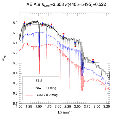
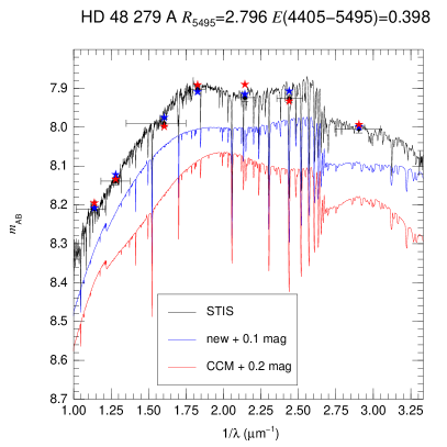
Two moderately extinguished Galactic O stars (AE Aur and HD 48 279 A with even better STIS coverage (G430L and G750L) than for the two 30 Doradus stars in the previous subsection are present in the HST archive thanks to the Next Generation Spectral Library (Gregg et al., 2004). The spectra were reprocessed and calibrated in flux using Tycho-2 photometry (Maíz Apellániz, 2005, 2006, 2007). We derived synthetic photometry from the spectrophotometry, estimated their from their spectral types (Sota et al., 2011), and applied CHORIZOS in a manner equivalent to experiments 1 (CCM) and 3 (new)888With one difference: we fix the luminosity class and leave distance as a free parameter.. Results are shown in Figure 9.
The most obvious conclusion from Figure 9 is that the new extinction laws reproduce the detailed behavior of the extinction law in the optical range better than the CCM ones: once again, splines beat a seventh degree polynomial. In particular, the behavior around the Whitford (1958) 2.2 m-1 knee and the band (1.6 m-1) is better reproduced. Another positive conclusion is that the Balmer jump for these later-type O stars is also well reproduced by the TLUSTY models, another indication that it is not the source of discrepancies for in experiments 2 and 4. There are also two not-so-positive conclusions. The first one is that the detailed wavelength behavior of HD 48 279 A fit with the new laws is not as good as the one for AE Aur (though it is still a slight improvement over the CCM fit). This is not a surprising conclusion because the value of for HD 48 279 A is outside the range measured in 30 Doradus while the one for AE Aur is inside: extrapolated laws are more uncertain than interpolated ones. The second one is the realization that TLUSTY models (at least those of Lanz & Hubeny 2003, 2007, note that in this case we are using the grid with MW metallicity, not the LMC one) do not treat the Paschen jump correctly, apparently because they do not include the higher-order transitions. Hence, one should be careful when analyzing photometry with TLUSTY models.
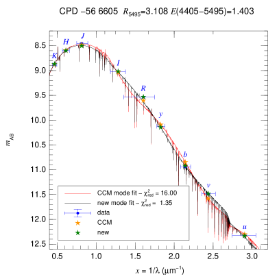
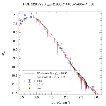
What about higher extinctions? We searched the Galactic O-Star Catalog (Maíz Apellániz et al., 2004b; Sota et al., 2008) for O stars with mag and good-quality Strömgren and 2MASS photometry999The reason for preferring Strömgren to Johnson photometry is that the use of two filters () in the -band region makes the first system more sensitive to the behavior of the extinction law across the Whitford (1958) 2.2 m-1 knee.. We found two stars, CPD 56 6605 and HDE 228 779, that met the requirements; the first one also has Cousins photometry available. Neither of the two stars is included in the first two papers (Sota et al., 2011, 2014) of the Galactic O-Star Spectroscopic Survey (Maíz Apellániz et al., 2011), but the project has already obtained their spectra and classified them as O9.7 Iab and O9 Iab, respectively, hence allowing us to derive their . With that information, we performed the CHORIZOS experiments in analogy to the ones for AE Aur and HD 48 279 A. Results are shown in Figure 10.
Once again, the new laws beat the CCM ones by a large margin. The CCM values for of 16.00 and 20.08 for the two stars are reduced to 1.35, and 2.38, respectively. Also, the detailed wavelength behavior of the new SED does not show the wiggles present in the CCM one. Therefore, at least for these two cases the new laws provide a good fit to heavily extinguished O stars with standard values of (3.0-3.1)101010The difference between the two extinction law families is, in general, small for quantities that depend on the value of (e.g. magnitudes and ), larger for those that depend on its first derivative (e.g. colors), and even larger for those that depend on its second derivative (e.g. Strömgren and indices)..
5 Guidelines and future work
When applying the extinction laws in this paper, we recommend following these guidelines:
-
•
In general, passband effects (differences between the extinction measured at the central wavelength of a filter and the extinction integrated over the whole passband) can be significant (Maíz Apellániz 2013a and references therein), especially for samples with large extinctions and differences in . Do not apply simple linear extinction corrections (e.g. -like parameters) in these cases. Instead, integrate over the whole passband using the routine in Table 2 or its equivalent.
-
•
In the optical, the extinction laws have been tested on a limited sample up to mag. Future studies may improve the results here, though it would be surprising if an optical extinction with an overall dependence with wavelength very different from the ones here or in CCM were discovered.
-
•
The NIR law used here is the power law of Rieke & Lebofsky (1985). A large number of works since then (e.g. Moore et al. 2005; Fitzpatrick & Massa 2009; Fritz et al. 2011) have found different values of the power law exponent and possible changes between sightlines so, strictly speaking, the laws here should not be applicable. However, for low and intermediate reddenings mag, NIR extinction corrections should be small enough to yield acceptable differences. In other words, in the NIR apply these laws to optically visible OB stars, not to targets in the Galactic Center.
-
•
It is well known that the extinction law in the MIR and FIR is not a power law. Do not apply the results here in that range (that is the reason why the routine in Table 2 does not accept values below m-1).
-
•
UV extinction is a different and difficult issue111111For example, Fitzpatrick & Massa (2007) find that there is no strong correlation between the UV and the IR Galactic extinctions, in opposition to what CCM found. More recently, Peek & Schiminovich (2013) have found that at high Galactic latitudes UV extinction is anomalous and suggested a connection with an increase in the amount of very small silicate grains. that is not measured in this paper even though a functional form is provided. More specifically, the routine in Table 2 may work for low values of (as CCM does) but is guaranteed to fail for high values of . The reason is that the jump seen for = 5.0 and 7.0 around m-1 is not physical but a product of tying up the results of this paper in the optical with those of CCM in the UV.
Our future work will develop along the following lines:
-
•
We will analyze the spatial distribution of dust in 30 Doradus in a subsequent paper of the VFTS series. In particular, we will study the dependence of with the environment.
-
•
We will apply the optical and NIR extinction laws in this paper to a number of existing datasets. In particular, we will use them to measure the amount and type of extinction in the GOSSS stars (Maíz Apellániz et al., 2011).
-
•
We will use spectrophotometry to check the detailed behavior in of the extinction laws.
-
•
We will obtain data for stars with mag to test the relationship between and the NIR slope.
Acknowledgements.
This article is based on observations at the European Southern Observatory Very Large Telescope in programme 182.D-0222 and on observations made with the NASA/ESA Hubble Space Telescope (HST) associated with GO program 11 360 and obtained at the Space Telescope Science Institute, which is operated by the Association of Universities for Research in Astronomy, Inc., under NASA contract NAS 5-26 555. We would like to thank Max Mutchler for helping with the processing of the WFC3 images. J.M.A. acknowledges support from [a] the Spanish Government Ministerio de Economía y Competitividad (MINECO) through grants AYA2010-15 081 and AYA2010-17 631, [b] the Consejería de Educación of the Junta de Andalucía through grant P08-TIC-4075, and [c] the George P. and Cynthia Woods Mitchell Institute for Fundamental Physics and Astronomy. He is also grateful to the Department of Physics and Astronomy at Texas A&M University for their hospitality during some of the time this work was carried out. R.H.B. acknowledges support from DIULS and FONDECYT Project 1 120 668. A.H. and S.S.-D. acknowledge funding by [a] the Spanish Government Ministerio de Economía y Competitividad (MINECO) through grants AYA2010-21 697-C05-04, AYA2012-39 364-C02-01, and Severo Ochoa SEV-2011-0187 and [b] the Canary Islands Government under grant PID2 010 119.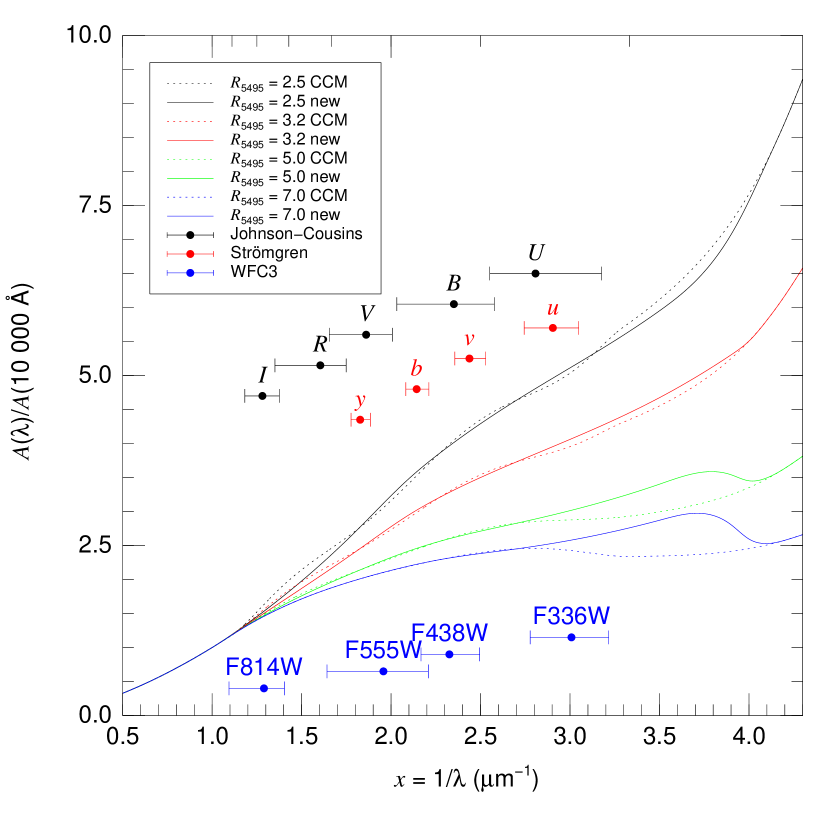
References
- Arias et al. (2010) Arias, J. I., Barbá, R. H., Gamen, R. C., et al. 2010, ApJL, 710, L30
- Arias et al. (2006) Arias, J. I., Barbá, R. H., Maíz Apellániz, J., Morrell, N. I., & Rubio, M. 2006, MNRAS, 366, 739
- Blanco (1957) Blanco, V. M. 1957, ApJ, 125, 209
- Cardelli et al. (1989) Cardelli, J. A., Clayton, G. C., & Mathis, J. S. 1989, ApJ, 345, 245
- Cioni et al. (2011) Cioni, M.-R., Clementini, G., Girardi, L., et al. 2011, The Messenger, 144, 25
- De Marchi et al. (2011) De Marchi, G., Paresce, F., Panagia, N., et al. 2011, ApJ, 739, 27
- Doran et al. (2013) Doran, E. I., Crowther, P. A., de Koter, A., et al. 2013, A&A, 558, A134
- Evans et al. (2011) Evans, C. J., Taylor, W. D., Hénault-Brunet, V., et al. 2011, A&A, 530, A108
- Fitzpatrick (1985) Fitzpatrick, E. L. 1985, ApJ, 299, 219
- Fitzpatrick (1999) Fitzpatrick, E. L. 1999, PASP, 111, 63
- Fitzpatrick & Massa (2005) Fitzpatrick, E. L. & Massa, D. 2005, AJ, 130, 1127
- Fitzpatrick & Massa (2007) Fitzpatrick, E. L. & Massa, D. 2007, ApJ, 663, 320
- Fitzpatrick & Massa (2009) Fitzpatrick, E. L. & Massa, D. 2009, ApJ, 699, 1209
- Fritz et al. (2011) Fritz, T. K., Gillessen, S., Dodds-Eden, K., et al. 2011, ApJ, 737, 73
- Gordon & Clayton (1998) Gordon, K. D. & Clayton, G. C. 1998, ApJ, 500, 816
- Gregg et al. (2004) Gregg, M. D., Silva, D., Rayner, J., et al. 2004, American Astronomical Society Meeting Abstracts, 205
- Howarth (1983) Howarth, I. D. 1983, MNRAS, 203, 301
- Hummer et al. (1988) Hummer, D. G., Abbott, D. C., Voels, S. A., & Bohannan, B. 1988, ApJ, 328, 704
- Kato et al. (2007) Kato, D., Nagashima, C., Nagayama, T., et al. 2007, PASJ, 59, 615
- Laidler et al. (2005) Laidler, V. et al. 2005, Synphot User’s Guide v5.0 (STScI: Baltimore)
- Lanz & Hubeny (2003) Lanz, T. & Hubeny, I. 2003, ApJS, 146, 417
- Lanz & Hubeny (2007) Lanz, T. & Hubeny, I. 2007, ApJS, 169, 83
- Maíz Apellániz (2004) Maíz Apellániz, J. 2004, PASP, 116, 859
- Maíz Apellániz (2005) Maíz Apellániz, J. 2005, PASP, 117, 615
- Maíz Apellániz (2006) Maíz Apellániz, J. 2006, AJ, 131, 1184
- Maíz Apellániz (2007) Maíz Apellániz, J. 2007, in ASP Conf. Series, Vol. 364, The Future of Photometric, Spectrophotometric and Polarimetric Standardization, ed. C. Sterken, 227
- Maíz Apellániz (2013a) Maíz Apellániz, J. 2013a, in Highlights of Spanish Astrophysics VII, 583–589
- Maíz Apellániz (2013b) Maíz Apellániz, J. 2013b, in Highlights of Spanish Astrophysics VII, 657–657
- Maíz Apellániz et al. (2004a) Maíz Apellániz, J., Bond, H. E., Siegel, M. H., et al. 2004a, ApJL, 615, 113
- Maíz Apellániz & Rubio (2012) Maíz Apellániz, J. & Rubio, M. 2012, A&A, 541, A54
- Maíz Apellániz & Sota (2008) Maíz Apellániz, J. & Sota, A. 2008, in Rev. Mex. Astron. Astrofís. (conference series), Vol. 33, 44–46
- Maíz Apellániz et al. (2011) Maíz Apellániz, J., Sota, A., Walborn, N. R., et al. 2011, in Highlights of Spanish Astrophysics VI, ed. M. R. Zapatero Osorio, J. Gorgas, J. Maíz Apellániz, J. R. Pardo, & A. Gil de Paz, 467–472
- Maíz Apellániz et al. (2004b) Maíz Apellániz, J., Walborn, N. R., Galué, H. Á., & Wei, L. H. 2004b, ApJS, 151, 103
- Maíz Apellániz et al. (2007) Maíz Apellániz, J., Walborn, N. R., Morrell, N. I., Niemelä, V. S., & Nelan, E. P. 2007, ApJ, 660, 1480
- Martins et al. (2005) Martins, F., Schaerer, D., & Hillier, D. J. 2005, A&A, 436, 1049
- Misselt et al. (1999) Misselt, K. A., Clayton, G. C., & Gordon, K. D. 1999, ApJ, 515, 128
- Mokiem et al. (2007) Mokiem, M. R., de Koter, A., Evans, C. J., et al. 2007, A&A, 465, 1003
- Moore et al. (2005) Moore, T. J. T., Lumsden, S. L., Ridge, N. A., & Puxley, P. J. 2005, MNRAS, 359, 589
- Negueruela et al. (2006) Negueruela, I., Smith, D. M., Harrison, T. E., & Torrejón, J. M. 2006, ApJ, 638, 982
- Pasquini et al. (2002) Pasquini, L., Avila, G., Blecha, A., et al. 2002, The Messenger, 110, 1
- Peek & Schiminovich (2013) Peek, J. E. G. & Schiminovich, D. 2013, ApJ, 771, 68
- Prévot et al. (1984) Prévot, M. L., Lequeux, J., Maurice, E., Prévot, L., & Rocca-Volmerange, B. 1984, A&A, 132, 389
- Rieke & Lebofsky (1985) Rieke, G. H. & Lebofsky, M. J. 1985, ApJ, 288, 618
- Rubele et al. (2012) Rubele, S., Kerber, L., Girardi, L., et al. 2012, A&A, 537, A106
- Rubio et al. (1998) Rubio, M., Barbá, R. H., Walborn, N. R., et al. 1998, AJ, 116, 1708
- Sabín-Sanjulián et al. (2013) Sabín-Sanjulián, C., Simón-Díaz, S., Herrero, A., et al. 2013, ArXiv e-prints
- Sana et al. (2013) Sana, H., de Koter, A., de Mink, S. E., et al. 2013, A&A, 550, A107
- Schaerer et al. (1993) Schaerer, D., Meynet, G., Maeder, A., & Schaller, G. 1993, A&AS, 98, 523
- Schaller et al. (1992) Schaller, G., Schaerer, D., Meynet, G., & Maeder, A. 1992, A&AS, 96, 269
- Simón-Díaz et al. (2011) Simón-Díaz, S., Castro, N., Herrero, A., et al. 2011, Journal of Physics Conference Series, 328, 012021
- Skrutskie et al. (2006) Skrutskie, M. F., Cutri, R. M., Stiening, R., et al. 2006, AJ, 131, 1163
- Sota et al. (2014) Sota, A., Maíz Apellániz, J., Morrell, N. I., et al. 2014, ArXiv e-prints
- Sota et al. (2011) Sota, A., Maíz Apellániz, J., Walborn, N. R., et al. 2011, ApJS, 193, 24
- Sota et al. (2008) Sota, A., Maíz Apellániz, J., Walborn, N. R., & Shida, R. Y. 2008, in Rev. Mex. Astron. Astrofís. (conference series), Vol. 33, 56
- Tatton et al. (2013) Tatton, B. L., van Loon, J. T., Cioni, M.-R., et al. 2013, A&A, 554, A33
- Úbeda et al. (2007) Úbeda, L., Maíz Apellániz, J., & MacKenty, J. W. 2007, AJ, 133, 917
- van Loon et al. (2013) van Loon, J. T., Bailey, M., Tatton, B. L., et al. 2013, A&A, 550, A108
- Walborn et al. (1999) Walborn, N. R., Barbá, R. H., Brandner, W., et al. 1999, AJ, 117, 225
- Walborn et al. (2002) Walborn, N. R., Maíz Apellániz, J., & Barbá, R. H. 2002, AJ, 124, 1601
- Walborn et al. (2014) Walborn, N. R., Sana, H., Simón-Díaz, S., et al. 2014, A&A (accepted)
- Whitford (1958) Whitford, A. E. 1958, AJ, 63, 201
Appendix A The new extinction laws
Based on the issues discussed in Maíz Apellániz (2013a) and the results of experiments 1 and 2, we decided to attempt the calculation of a new family of extinction laws. Ideally, to complete such a task one would use high-quality spectrophotometry from the NIR to the UV of a diverse collection of sources in different environments and with different degrees of extinction. Since such dataset is not available, in this paper we concentrate on only some of the problems discussed in Maíz Apellániz (2013a). More specifically, we will ignore extinction in the UV (except for the region closest to the optical) and for the NIR we will simply use the CCM laws (which, in turn, used Rieke & Lebofsky 1985)121212We have verified that our values of and are compatible with the Rieke & Lebofsky (1985) value for the NIR exponent and with the TLUSTY SEDs yielding the correct intrinsic colors for OB stars with LMC metallicity. Note, however, that given the low values of the NIR extinction of the stars in our sample, there is not enough information to discard alternatives.. In other words, we will concentrate on the optical region since that is the critical component for the determination of for OB stars. Ignoring the UV will not matter to a non-specialist interested only in eliminating the extinction from his/her optical data. Ignoring the NIR may matter if the exponent there is significantly different from the CCM one but only if extinction is very large and even then it may only apply to the total extinction correction, not to the determination of from the photometry.
The immediate goals of the new family of extinction laws are:
-
1.
To maintain the overall properties of the CCM laws that have made them so successful: a single-parameter, easy-to-calculate family that covers a large wavelength range; and their overall shape as a function of wavelength (including the functional form in Eqn. 4).
-
2.
To eliminate the F336W (-band like) excesses detected in experiment 1, which lead to the temperature biases in experiment 2.
-
3.
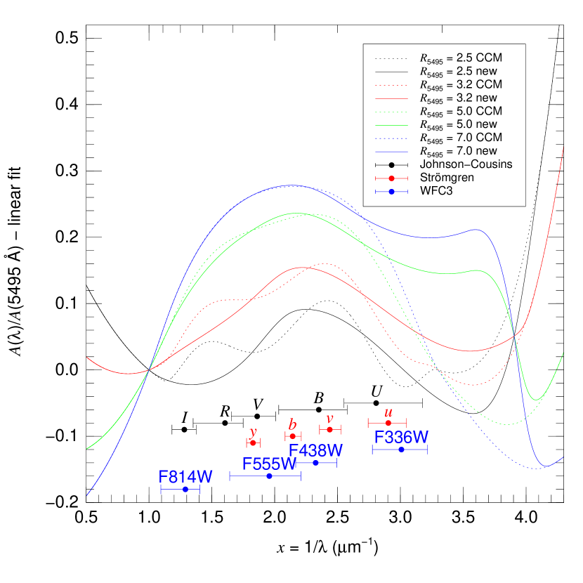
To at least alleviate the wiggles induced by the seventh-degree polynomial used by CCM in the optical range and make the new family more similar to the shape derived by Whitford (1958) with spectrophotometry (two straight lines with a knee at m-1).
To achieve those goals, we use the following strategy:
-
1.
Instead of a seventh-degree polynomial, we [a] select a series of points in in the optical range, [b] use the values of the CCM laws at these points (with corrections in some cases), and [c] apply a spline interpolation between these points. Note that a spline interpolation was already used by Fitzpatrick (1999).
-
2.
We expand the optical range from = 1.1-3.3 m-1 to 1.0-4.2 m-1 in order to avoid discontinuities and/or knees near the edges of the ranges131313Note that such knees exist for low values of in the CCM laws, see the = 2.5 case in Fig. 12..
-
3.
The first two points selected are = 1.81984 m-1 and = 2.27015 m-1, which correspond to 5495 Å and 4405 Å. The choice is determined by the need to maintain the values of for a given extinction law. At these values no correction is applied to the CCM laws.
-
4.
A third point is added between = 1.81984 m-1 and = 1.0 m-1 to minimize the wiggles visible for low and intermediate values of in CCM and thus make the extinction laws more similar to that of Whitford (1958). After trying different choices, we select m-1 as the one that produces the smoothest results. Note that the values of the extinction law at exactly these three points are the CCM ones: the changes affect the points in between due to the use of a spline interpolation instead of a seventh-degree polynomial.
-
5.
A fourth point is added between 5495 Å and 4405 Å to maintain the Whitford (1958) knee at its original location near = 2.2 m-1 (as it can be seen in Fig. 11, CCM moved the knee towards higher values, i.e. shorter wavelengths, in most cases while the new laws put it back between 2.15 m-1 and 2.25 m-1 for most values of ). By trial and error we selected = 2.1 m-1 and applied a correction to the / CCM values there of .
-
6.
Five final points are added between = 2.27015 m-1 and = 4.2 m-1. Different combinations were tried with the general goals of [a] keeping smooth profiles, [b] correcting the overall F336W excesses found in experiment 1 as a function of , and [c] doing the same as a function of . The final result leads to the points being located at = 2.7 m-1, 3.5 m-1, 3.9 m-1, 4.0 m-1, and 4.1 m-1. The corrections to / in these points are 0, , , , and , respectively. Note that the optical region in CCM ends at = 3.3 m-1: for higher values of the correction is applied to the CCM UV functional form.
Four examples of the new extinction laws are shown in Figs. 11 and 12. An IDL function to obtain the new extinction laws is provided in Table 2. The validity of the new extinction laws is tested in experiments 3 and 4 i.e. the ones used to iteratively determine them.
FUNCTION ALA5495, lambda, R5495=r5495
; This function gives A_lambda/A_5495 for the range 1000 Angstroms - 33 333 Angstroms
;  (3.333 3 microns) according to the Ma\’{\i}z Apell\’aniz et al. (2014) extinction laws.
; Positional parameters:
; lambda:   Wavelength in Angstroms (single value or array).
; Keyword parameters:
; R5495:   R_5495 value. By default, it is 3.1.
IF KEYWORD_SET(R5495) EQ 0 THEN r5495 = 3.1
x   = 10000D/lambda
n   = N_ELEMENTS(x)
IF MIN(x) LT 0.3 OR MAX(x) GT 10.0 THEN STOP, ’Wavelength not implemented’
; Infrared
ai  =   0.574*x^1.61
bi  = - 0.527*x^1.61
; Optical
x1  = [1.0]
xi1 = x1[0]
x2  = [1.15,1.81984,2.1,2.27015,2.7]
x3  = [3.5 ,3.9    ,4.0,4.1    ,4.2]
xi3 = x3[N_ELEMENTS(x3)-1]
a1v =   0.574      *x1^1.61
a1d =   0.574*1.61*xi1^0.61
b1v = - 0.527      *x1^1.61
b1d = - 0.527*1.61*xi1^0.61
a2v =  1 + 0.17699*(x2-1.82)   - 0.50447*(x2-1.82)^2 - 0.02427*(x2-1.82)^3 + 0.72085*(x2-1.82)^4 $
         + 0.01979*(x2-1.82)^5 - 0.77530*(x2-1.82)^6 + 0.32999*(x2-1.82)^7 + [0.0,0.0,-0.011,0.0,0.0]
b2v =      1.41338*(x2-1.82)   + 2.28305*(x2-1.82)^2 + 1.07233*(x2-1.82)^3 - 5.38434*(x2-1.82)^4 $
         - 0.62251*(x2-1.82)^5 + 5.30260*(x2-1.82)^6 - 2.09002*(x2-1.82)^7 + [0.0,0.0,+0.091,0.0,0.0]
a3v =   1.752 - 0.316*x3 - 0.104/             (( x3-4.67)*( x3-4.67) + 0.341) + [0.442,0.341,0.130,0.020,0.000]
a3d =         - 0.316    + 0.104*2*(xi3-4.67)/((xi3-4.67)*(xi3-4.67) + 0.341)^2
b3v = - 3.090 + 1.825*x3 + 1.206/             (( x3-4.62)*( x3-4.62) + 0.263) - [1.256,1.021,0.416,0.064,0.000]
b3d =         + 1.825    - 1.206*2*(xi3-4.62)/((xi3-4.62)*(xi3-4.62) + 0.263)^2
as  =           SPL_INIT([x1,x2,x3], [a1v,a2v,a3v], YP0=a1d, YPN_1=a3d)
bs  =           SPL_INIT([x1,x2,x3], [b1v,b2v,b3v], YP0=b1d, YPN_1=b3d)
av  = REVERSE(SPL_INTERP([x1,x2,x3], [a1v,a2v,a3v], as, REVERSE(x)))
bv  = REVERSE(SPL_INTERP([x1,x2,x3], [b1v,b2v,b3v], bs, REVERSE(x)))
; Ultraviolet
y   = x - 5.9
fa  = REPLICATE(0.0D,n) + (- 0.04473*y^2 - 0.009779*y^3)*(x LE 8.0 AND x GE 5.9)
fb  = REPLICATE(0.0D,n) + (   0.2130*y^2 +   0.1207*y^3)*(x LE 8.0 AND x GE 5.9)
au  =   1.752 - 0.316*x - 0.104/((x-4.67)*(x-4.67) + 0.341) + fa
bu  = - 3.090 + 1.825*x + 1.206/((x-4.62)*(x-4.62) + 0.263) + fb
; Far ultraviolet
y   = x - 8.0
af  = -  1.073 - 0.628*y + 0.137*y^2 - 0.070*y^3
bf  =   13.670 + 4.257*y - 0.420*y^2 + 0.374*y^3
; Final result
a   = ai*(x LT xi1) + av*(x GE xi1 AND x LT xi3) + au*(x GE xi3 AND x LT 8.0) + af*(x GE 8.0)
b   = bi*(x LT xi1) + bv*(x GE xi1 AND x LT xi3) + bu*(x GE xi3 AND x LT 8.0) + bf*(x GE 8.0)
RETURN, a + b/r5495
END
Appendix B CHORIZOS and SED models
The code CHORIZOS was presented in Maíz Apellániz (2004) as a Code for Parameterized Modeling and Characterization of Photometry and Spectrophotometry. In subsequent versions, it evolved to become a complete bayesian code that matches photometry and spectrophotometry to spectral energy distribution (SED) models in up to six dimensions. Some examples of its applications can be seen in Maíz Apellániz et al. (2004a); Maíz Apellániz et al. (2007); Negueruela et al. (2006); Úbeda et al. (2007). The last public version of CHORIZOS, v. 2.1.4, was released in July 2007. Since then, the first author of this paper has been working on versions 3.x, which, among many changes, allow for the use of magnitudes (instead of colors) as fitting quantities and the use of distance as an additional parameter. Problems with the code speed and memory usage did not allow these versions of CHORIZOS to become public (even though the code itself worked for restricted cases). The largest problems have now been solved and a public application with the 3.x version of the code will be publicly available soon.
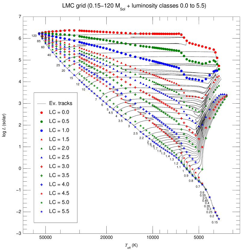
The use of magnitudes and distances described above leads to the possibility of a new type of stellar SED grids: instead of using and as the two parameters, one can substitute by luminosity or an equivalent parameter (Maíz Apellániz 2013b). As an intermediate step, one needs to use evolutionary tracks or isochrones that assign the correct value of to a given luminosity. We have developed a class of such grids with the following characteristics:
-
1.
There are three separate grids corresponding to the Milky Way, LMC (the ones used in this paper), and SMC metallicities.
-
2.
The luminosity-type parameter is called (photometric) luminosity class and is analogous to the spectroscopic equivalent. To maintain the equivalence as close as possible, its value ranges from 0.0 (hypergiants) to 5.5 (ZAMS).
-
3.
The grids use Geneva evolutionary tracks for high-mass stars and Padova ones for intermediate- and low-mass stars. For the objects in this paper, the relevant tracks are those of Schaller et al. (1992); Schaerer et al. (1993). Note that the use of tracks with rotation would not introduce significant changes in the results of this paper because the purpose of the tracks for O stars are to [a] establish the total range in luminosities and [b] determine the gravity for a given temperature and luminosity. The range in luminosities changes little with the introduction of rotation and the possible changes in gravity at a given grid point can be of the order of 0.2 dex, which leads to an insignificant effect in the optical colors of O stars141414There are some cases (very high mass, extreme ) where rotation does matter but they are not relevant to this paper..
- 4.
-
5.
It is possible to specify a total of five parameters in a given grid: , luminosity class, , , and distance. Note, however, that for most practical applications it is only possible to leave four of these parameters free.
-
6.
For the experiments in this paper we have calculated independent grids with the CCM, F99, and new extinction laws.
Figure 13 shows the LMC grid used in this paper.
Appendix C Extinction along a sightline with more than one type of dust
In this paper we make no attempt to disentangle the contributions to the extinction in 30 Doradus among its three possible components: Milky Way (MW), Large Magellanic Cloud (LMC), and internal (30 Dor). The reason for not attempting to do so is the impossibility of doing it with the available data (each component can contribute while being spatially variable, see van Loon et al. 2013). However, that does not affect the validity of our results due to a feature of the extinction law families of CCM and this paper. The extinction laws are written as:
| (4) |
where and are defined by different functional forms in different wavelength ranges (see e.g. Table 2). A SED with an original form of is extinguished to according to:
| (5) |
Now, suppose that along the sightline to a star there are clouds, each one of them with a color excess and type of extinction . The total extinction will be:
| (6) |
| (7) |
| (8) |
i.e. if each individual extinction law belongs to the same family, then it will represent the combined effect of the clouds. The total color excess is simply the sum of the individual ones and the type of extinction is the sum of the individual types (characterized by their values) weighted by the individual color excesses.