Magnetar Giant Flares in Multipolar Magnetic Fields —
I. Fully and Partially Open Eruptions of Flux Ropes

Abstract

We propose a catastrophic eruption model for magnetar’s enormous energy release during giant flares, in which a toroidal and helically twisted flux rope is embedded within a force-free magnetosphere. The flux rope stays in stable equilibrium states initially and evolves quasi-statically. Upon the loss of equilibrium point is reached, the flux rope cannot sustain the stable equilibrium states and erupts catastrophically. During the process, the magnetic energy stored in the magnetosphere is rapidly released as the result of destabilization of global magnetic topology. The magnetospheric energy that could be accumulated is of vital importance for the outbursts of magnetars. We carefully establish the fully open fields and partially open fields for various boundary conditions at the magnetar surface and study the relevant energy thresholds. By investigating the magnetic energy accumulated at the critical catastrophic point, we find that it is possible to drive fully open eruptions for dipole dominated background fields. Nevertheless, it is hard to generate fully open magnetic eruptions for multipolar background fields. Given the observational importance of the multipolar magnetic fields in the vicinity of the magnetar surface, it would be worthwhile to explore the possibility of the alternative eruption approach in multipolar background fields. Fortunately, we find that flux ropes may give rise to partially open eruptions in the multipolar fields, which involve only partial opening up of background fields. The energy release fractions are greater for cases with central-arcaded multipoles than those with central-caved multipoles emerged in background fields. Eruptions would fail only when the centrally-caved multipoles become extremely strong.

1 Introduction

Two small subsets of neutron stars $-$ anomalous X-ray pulsars (AXPs) and soft gamma-ray repeaters (SGRs) are interpreted as magnetars, which are neutron stars endowed with ultra-strong ($10^{14}-10^{15}$G) magnetic fields (Mazets et al., 1979; Mereghetti & Stella, 1995; Kouveliotou et al., 1998; Gavriil et al., 2002). The magnetic energy dissipation is commonly believed to account for their high energy persistent emissions and spasmodic outbursts (Duncan & Thompson, 1992; Woods & Thompson, 2006; Mereghetti, 2008). One of the most intriguing phenomena related to magnetars is the episodic giant flare, which involves tremendous magnetic energy release (Hurley et al., 2005). The physical origin of giant flares still remains the bewildering enigma in high energy astrophysics. The magnetospheric eruption models (e.g., Lyutikov, 2006; Gill & Heyl, 2010; Yu, 2012; Yu & Huang, 2013) can naturally explain the short timescale, $\sim 0.25$ms, of the rise time in giant flares (Palmer et al., 2005), although the precise mechanism of the eruption is still under debate (Mereghetti, 2013). It is worthwhile to note that, in the magnetospheric eruption model, the magnetosphere stays in a stable equilibrium state at the pre-eruptive stage, in which the magnetosphere evolves quasi-statically. As a result, the magnetic energy released in an eruption is gradually accumulated on a timescale much longer the dynamical timescale of giant flares. Since the energy accumulation takes place very gradually, the question how such long timescale events could initiate the sudden energy release, i.e., giant flares, on a very short dynamical timescale, remains elusive for the magnetospheric eruption model.

To resolve this puzzle, a catastrophic flux rope eruption model has been put forward to explain the magnetar giant flare (Yu, 2012; Yu & Huang, 2013). In this particular scenario, the giant flare is considered to be driven by the destabilization of large-scale magnetospheric magnetic fields rather than the abrupt fracture of the neutron star crust. The most distinguishing feature in our model is that a helically twisted flux rope is embedded within the magnetosphere. Magnetic flux ropes could be naturally generated due to the the magnetic helicity injections from the magnetar interior (Thompson et al .2002; Lyutikov 2006; Götz et al. 2007; Gill & Heyl 2010). Such flux ropes are also an indispensable ingredient to explain the radio afterglow of SGR1806 (Gaensler et al., 2005; Lyutikov, 2006). It is interesting to note that the interior of the flux rope is helically twisted. The magnetic twist is locally confined within the flux rope, which is at variance with the global twist proposed by recent authors (Lyutikov, 2013; Parfrey et al., 2013). These locally twisted magnetic features, when compared to the global twist, seem to be more relevant to the recent observations (e.g., Woods et al., 2007; Perna & Gotthelf, 2008).

The flux rope eruption model tries to resolve a primary issue concerning the trigger mechanism of the magnetar eruption. The most appealing characteristic is that, during the flux rope’s evolution, it could make the catastrophic state transition from stable equilibrium states to unstable equilibrium states spontaneously in accordance with the variations at the neutron star surface. The emergence of flux from the interior (Kluźniak & Ruderman, 1998; Götz et al., 2007) and/or the shuffling of the crust (Ruderman, 1991) causes the flux rope to evolve to a critical loss of equilibrium point, beyond which no stable equilibrium state can be sustained and the flux rope erupts abruptly. It is widely accepted that the energy is progressively accumulated in an initially closed force-free field before the flux rope reaches the critical loss of equilibrium point. The flux rope’s subsequent catastrophic eruption, beyond this particular point, leads to the opening up of initially closed magnetic field configuration as well as huge energy release. Since the stored energy prior to an eruption is determined by the intrinsic properties of the magnetosphere rather than the tensile strength of the crust (Yu, 2012), a fundamental question is raised naturally as to whether the magnetic energy in the force free magnetosphere could build up enough energy to support eruptive giant flares.

The fierce eruptive event is thought to open up the pre-eruptive, originally closed magnetic field lines. Observationally, in the post-eruption epoch of giant flares, magnetic field configurations are indeed inferred to stretch outwards to form an open field structure (e.g. Wood et al., 2001). From the perspective of energy budget, a closed field configuration is physically favored for giant flares only if the magnetic energy stored in magnetosphere can exceeds that stored in an open field configuration. In other words, in addition to power the giant flares, the magnetic free energy has to be able to open up the initially closed magnetic fields. This constitutes a serious bottleneck for magnetar giant flares because it is realized that to open up the initially closed field lines requires considerable extra work to be done (Aly, 1984, 1991; Sturrock, 1991; Yu, 2012). To get over the energy threshold constrained by the post-eruptive open field configurations, the pre-eruptive magnetosphere must accumulate more energy in excess of the threshold set by the open field configurations. It should be pointed out that the field lines can also be opened up at a greater distance from the star by strong neutron star winds (e.g., Bucciantini et al., 2006). How the wind affect the magnetar eruption energetics is still an open issue. For simplicity, we only consider the case in which the field lines are opened up by the process of magnetic flux injection from the neutron star interior.

The observational feature of strong four-peaked pattern in the pulse profile of the 1998 August 27 event from SGR 1900+14 indicates that the geometry of the magnetic field was quite complicated in regions close to the star (Feroci et al., 2001). Recent calculations also show that multipolar magnetic fields may also have important effects on the emission of the magnetars (Pavan et al., 2009). As a result, it is reasonable to infer that, in the very vicinity of the magnetar surface, the field configuration involves higher multipoles. The electric currents formed during the birth of magnetars slowly push out from within the magnetar and generate active regions on the magnetar surface. These active regions manifest themselves as the multipolar regions on the magnetar surface. The flux rope eruption in multipolar background fields, unlike the behavior in dipole background fields, may just involve opening-up of part of the closed magnetic flux systems. Thus, it is interesting to explore the physical behavior of the flux rope in response to these more complex boundary conditions. However, for more complex boundary conditions, no solid investigations about the energy threshold specified by the fully/partially open field configurations have been performed. A related question, which is of crucial significance for the physical feasibility of the flux rope eruption model, i.e., whether the flux rope could build up enough energy to drive the giant flare with these complex boundary conditions, also remains to be answered.

In this paper, we will establish a force-free magnetosphere model with a helically twisted flux rope and examine the physical response of the flux rope to the variations of the background multi-polar magnetic fields. We perform rigorous calculations on the magnetic energy accumulation in magnetospheres in various configurations. Specifically, boundary conditions containing the dipolar term and the high order multipolar term are considered in the background closed magnetic field. Two kinds of open configurations, the partially open and fully open fields, are considered to provide energy thresholds for eruptions. This paper is structured as follows. The model of pre-eruptive magnetospheres with flux ropes and the multipolar boundary conditions are introduced in Section 2. The physical behavior of the pre-eruptive flux rope is described in Section 3, including the equilibrium constraints and catastrophic loss of equilibrium of the flux rope. The energetics of the flux rope in the multipolar background fields are investigated in Section 4. Conclusions and discussions are provided in Section 5.

2 Pre-eruptive Force-Free Magnetospheres With Embedded Flux Ropes

2.1 Force-Free Magnetospheres with Helically Twisted Flux Ropes

In our model, the most distinctive characteristic is that there exists a toroidal and helically twisted flux rope in the pre-eruptive magnetosphere. It is possible that the precursor activity of a giant flare may inject certain amount of magnetic helicity into the magnetosphere and generate such toroidal and helically twisted flux ropes (Thompson et al., 2002; Götz et al., 2007; Gill & Heyl, 2010). The toroidal flux rope has a major radius, $h$, which can be also understood as the height of the flux rope measured from the magnetar center, and a minor radius, $r_{0}$, which is small compared to $h$. The magnetic twist of the flux rope is confined within the flux rope, which is unlike the globally twisted magnetic fields configurations proposed by some authors (Thompson et al., 2002; Beloborodov, 2009; Parfrey et al., 2013; Lyutikov, 2013). These authors considered a non-potential force-free field where the electric currents flow through the entire magnetosphere. In comparison, our model only contains an electric current in a spatially restricted region, viz, inside the helically twisted flux rope. The magnetic field generated by the current inside the flux rope can be represented by a wire carrying a current $I$ at the center of the flux rope (Forbes & Priest, 1995).

The presence of the flux rope separates the magnetosphere into two regions, one is the region inside the flux rope. Further details about the solution inside the flux rope are discussed in Yu (2012). The other is the region outside the flux rope, in which the steady state axisymmetric magnetic field $\mathbf{B}$ takes the following form in spherical coordinates $(r,\theta,\phi)$

$$\mathbf{B} = -\frac{1}{r^{2}}\frac{\partial\Psi}{\partial\mu}\ \hat{\mathbf{e}}_{r}\ -\frac{1}{r\sin\theta}\frac{\partial\Psi}{\partial r}\ \hat{\mathbf{e}}_{\theta}\ ,$$ (1)

where $\Psi(r,\mu)$ is the magnetic stream function and $\mu=\cos\theta$. Here $\hat{\mathbf{e}}_{r}$ and $\hat{\mathbf{e}}_{\theta}$ are the unit vector along the radial and latitudinal direction, respectively. The force-free condition can be expressed in terms of the Grad-Shafranov (GS) equation, which explicitly reads ,

$$\frac{\partial^{2}\Psi}{\partial r^{2}}+\frac{(1-\mu^{2})}{r^{2}}\ \frac{\partial^{2}\Psi}{\partial\mu^{2}}\ =\ -r\sin\theta\ \frac{4\pi}{c}J_{\phi}\ ,$$ (2)

where $c$ is the speed of light and the current density $J_{\phi}$ on the right hand side in this inhomogeneous GS equation is induced by the toroidal flux rope, which is of the following form (Priest & Forbes, 2000; Yu, 2012)

$$J_{\phi}=\frac{I}{h}\ \delta(\mu)\ \delta(r-h)\ ,$$ (3)

where $I$ designates the electric current in the flux rope. According to the variable separation method, the general solution to the GS equation can be conveniently written as

$$\Psi(r,\mu) = \sum_{i=0}^{\infty}\bigg{[}c_{2i+1}R_{2i+1}(r)+d_{2i+1}r^{-2i-1}\bigg{]}\ \left[\frac{P_{2i}(\mu)-P_{2i+2}(\mu)}{4i+3}\right]\ ,$$ (4)

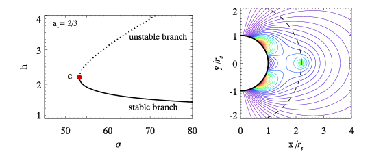
Figure 2: The same as Fig.1 but with a multipole-dominated background with $a_{1}=2/3$.

where $P_{2i}(\mu)$ is the Legendre polynomial and $R_{2i+1}(r)$ is a continuous function of $r$ (see Yu, 2011, 2012). The coefficients $c_{2i+1}$’s are determined by the current inside the flux rope. Once the magnetar surface boundary conditions are fixed, the coefficients $d_{2i+1}$’s can be readily specified in terms of $c_{2i+1}$’s and the boundary conditions. More technical details to obtain solutions of the GS equation can be found in Yu (2012). Once we obtain the spatial distribution of the magnetic stream function, the magnetic field configuration in the magnetosphere can be determined. Illustrative figures of the magnetic field configurations are shown in the panel $b$ of Fig.1 and Fig.2. The height of the flux rope (shown as dashed line) in these two fiugres is 1.27$r_{s}$ and 2.20$r_{s}$, respectively ($r_{s}$ is the magnetar radius, shown in thick solid line in these figures). In this paper we find that boundary conditions have important influences on the flux rope eruptions and in the following section we will further discuss the boundary conditions we adopt.

2.2 Multipolar Boundary Conditions and Post-Eruptive Energy Thresholds

The GS equation is solved in the range $[r_{s},\infty)$, where $r_{s}$ is the magnetar radius. The boundary conditions both at $r=r_{s}$ and $r\rightarrow\infty$ must be explicitly specified before we solve the GS equation (2). The physical requirement that $|\nabla\Psi|\rightarrow 0$ for $r\rightarrow\infty$ can be trivially satisfied (Yu, 2012). At the magnetar surface $r=r_{s}$, we adopt the multipolar boundary condition as (e.g., Antiochos et al., 1999; Zhang & Low, 2001)

$$\Psi(r_{s},\mu)=\Psi_{0}\sigma\Theta(\mu)\ ,$$ (5)

where $\Psi_{0}$ is a constant with magnetic flux dimension and the dimensionless variable $\sigma$ indicates the magnitude of magnetic flux at the magnetar surface. The large scale field configuration of the neutron star is essentially a dipole field. However, in the vicinity of the neutron star surface, which is exactly the location where the catastrophic loss of equilibrium takes place, the magnetic field may be more complicated than a simple dipole (Feroci et al., 2001). To model multipolar regions on the neutron star surface, we include high order multipolar components in addition to the dipole field and the angular dependence of the function $\Theta(\mu)$ can be written explicitly as

$$\Theta(\mu)=(1-\mu^{2})+a_{1}\ (5\mu^{2}-1)(1-\mu^{2})\ .$$ (6)

The first term $(1-\mu^{2})$ denotes the dipolar component of the magnetic fields and the additional term represents the contributions from high order multipolar components. The parameter $a_{1}$ determines the strength of the multipoles. The value of $a_{1}$ can be either positive or negative, the schematic illustration of the field configurations for different sign of $a_{1}$ are shown in middle- and bottom-left panels of Fig.6 in Appendix A. In this paper, we confine $a_{1}$ in the range of $[-1,1]$. Note that larger values of $|a_{1}|$ may indicate stronger magnetic activity of the magnetar (Kluźniak & Ruderman, 1998; Götz et al., 2007; Pavan et al., 2009).

In the post-eruption epoch of giant flares, magnetic field lines are stretched outwards to form open field structures (Wood et al., 2001). The possible post-eruptive open field configurations are specified by the profile of flux distribution at the magnetar surface. When the absolute value of the parameter $a_{1}$ is small, the background magnetic field is basically dipolar. The demarcation between dipole dominated fields and multipole dominated fields is determined by how many extremum points exist in the profile of the boundary flux distribution. More explicitly, if the parameter $a_{1}$ is in the range of $[-1/4,1/6]$, only one extremum point exits at $\mu=0$ in the boundary flux profile and the background magnetospheric field is essentially dipole dominated. Otherwise, the boundary flux function we take has three extremum points at $\mu_{0}=0$, $\mu_{1}=\sqrt{(6a_{1}-1)/10a_{1}}$, and $\mu_{2}=-\mu_{1}$, respectively (see Fig.6 in Appendix A). Due to the existence of the multiple extremum points, the multipolar configurations naturally arise in the background field. If $a_{1}\in(1/6,1]$, the background field has a central-caved profile on the boundary. If $a_{1}\in[-1,-1/4)$, the background field has a central-arcaded profile on the boundary. Note that for a dipole dominated background, there is only a single closed flux system in the magnetosphere (see in top-left panel in Fig.6.). The fully opening up of magnetic field specifically means the opening up of this particular closed flux system. However for a multipole dominated background, there are multiple closed flux systems in the magnetosphere (see in middle- and bottom-left panels in Fig.6.). The fully opening up of magnetic fields surely involves all the closed flux systems. However, it is possible that only part of the closed flux systems opens up and the post-eruptive field is then called partially open field. Details to obtain both the fully and partially open field configurations according to the boundary conditions we adopt are further discussed in Appendix A.

Throughout this work, the magnetic energy is scaled by the energy of the potential field satisfying $\nabla\times\mathbf{B}=0$, which has the minimum magnetic energy and is denoted by $W_{\rm pot}$. The magnetic energy of fully and partially open fields are denoted by $W^{\rm f}_{\rm open}$ and $W^{\rm p}_{\rm open}$, respectively. Further descriptions on how to calculate the magnetic energy of these two open states are given in Appendix B. The fully and partially open fields constitutes two energy thresholds, $W^{\rm f}_{\rm open}/W_{\rm pot}$ and $W^{\rm p}_{\rm open}/W_{\rm pot}$, for the flux rope eruptions. It is conceivable that the flux rope must accumulate enough magnetic energy to either fully or partially open up the initially closed fields. More specifically, the magnetic energy stored in the critical pre-eruptive state, $W_{\rm pre}(h_{c})/W_{\rm pot}$, should be larger than the fully or partially open threshold. Note that the magnetic energy of the critical pre-eruptive state, $W_{\rm pre}(h_{c})$, is closely related to the catastrophic behavior of the flux rope, which will be discussed in the following section.

3 Catastrophic Response of Flux Ropes to Variations at Magnetar Surface

It should be pointed out that, at the pre-eruptive stage, the flux rope stays in a stable equilibrium state and evolves quasi-statically with variations at the neutron star surface. During the pre-eruptive stage, the flux rope is unable to erupt and the magnetic energy is gradually accumulated in the magnetosphere. Upon the the critical loss of equilibrium point is reached, the quasi-static evolution is replaced by the subsequent dynamical evolution (Yu, 2012; Yu & Huang, 2013). The accumulated energy at the catastrophic loss of equilibrium point is of particular significance. This is because, beyond this point, no further gradual energy buildup is allowed and the flux rope’s dynamic behavior should be supported by the accumulated energy at this point. We denote the pre-eruptive energy at this loss of equilibrium point as $W_{\rm pre}$. To calculate the pre-eruptive state energy, $W_{\rm pre}$, it is necessary to know when the flux rope begins to lose its equilibrium.

3.1 Equilibrium Constranits of Flux Ropes

We adopt the the Lundquist (1950) force-free solution to represent the current density and field inside the toroidal flux rope. This solution, though originally derived for straight cylindrical twisted flux rope, is still valid as long as the minor radius $r_{0}$ is much smaller than the major radius, $h$. The axial magnetic flux conservation of the flux rope suggests that the minor radius $r_{0}$ is inversely proportional to the current carried by the flux rope $I$ (Yu 2012)

$$r_{0}=r_{00}I_{0}/I=r_{00}/J\ ,$$ (7)

where the dimensionless current $J$ is defined by $J\equiv I/I_{0}$. The scaling current $I_{0}=\Psi_{0}c/r_{s}$ is determined by the magnetic flux constant $\Psi_{0}$ in Equation (5), the magnetar radius $r_{s}$ and the speed of light $c$. For numerical conveniences, we scale the length by the magnetar radius $r_{s}$, magnetic flux by $\Psi_{0}$ and current by $I_{0}$ in our following calculations. The parameter $r_{00}$ is the value of $r_{0}$ when $J=1$. Typically for a flux rope with minor radius of $0.1$km, the value of the parameter $r_{00}\sim 0.01$ (We adopt the typical neutron star radius $r_{s}\sim 10$km).

In what follows, we consider slow responses of the flux rope to changes at the magnetar surface, and thus the flux rope is assumed to stay in a quasi-static equilibrium state on a sufficiently long timescale. Two aspects of the equilibrium constraint are considered, i.e., the force balance condition and the ideal frozen-flux condition. The force balance condition is satisfied when the total force exerted on the flux rope vanishes. The current inside the flux rope provides an outward force. The magnitude of this force is equal to the current, $I$, times the magnetic field, $B_{s}$ (Shafranov, 1966):

$$B_{s}=\frac{I}{ch}\left(\ln\frac{8h}{r_{0}}-1\right)\ ,$$ (8)

where $h$ and $r_{0}$ are the major and minor radius of the flux rope, respectively. This current-induced force must be balanced by the external magnetic field $B_{e}$. To calculate the external magnetic field $B_{e}$, the contribution from the current inside the flux rope must be excluded (Yu, 2012). Finally we can arrive at the mechanical force balance condition

$$f(\sigma,J,h)\equiv B_{s}-B_{e}=0\ ,$$ (9)

where the function $f(\sigma,J,h)$ can be written explicitly as

$$f(\sigma,J,h)=\frac{J}{h}\left(\ln\frac{8Jh}{r_{00}}-1\right)-\sum_{i=0}^{\infty}(2i+1)\left[\frac{P_{2i}(0)-P_{2i+2}(0)}{4i+3}\right]\frac{d_{2i+1}}{h^{2i+3}}\ .$$

We use $\sigma$ to represent the dimensionless magnitude of magnetic flux at the magnetar surface, $J$, the dimensionless current and $h$, the dimensionless height of the flux rope. Here the coefficients $d_{2i+1}$’s are already determined in Equation (4). Note that $P_{2i}(0)$ and $P_{2i+2}(0)$ are values of the Legendre polynomials at $\mu=0$.

The ideal frozen-flux condition must be also satisfied for the magnetic stream function, $\Psi$. It demands the stream function on the edge of the flux rope keep constant during the system’s evolution, which provides a connection between the variations at the magnetar surface and the current flowing inside the flux rope. Explicitly this condition can be written in the following form

$$g(\sigma,J,h)\equiv\Psi(h-r_{0},0)={\rm const}\ ,$$ (10)

where the function $g(\sigma,J,h)$ is defined by

$$g(\sigma,J,h)=\sum_{i=0}^{\infty}\left[\frac{P_{2i}(0)-P_{2i+2}(0)}{4i+3}\right]\left[c_{2i+1}\left(1-\frac{r_{00}}{Jh}\right)^{2i+2}+d_{2i+1}\left(h-\frac{r_{00}}{J}\right)^{-2i-1}\right]\ .$$

Note that the symbols in this equation has the same meaning as those in Equation (3.1) and the coefficients $c_{2i+1}$’s and $d_{2i+1}$’s are specified in Equation (4). With these two equations, the current $J$ and the height of the flux rope $h$ can be determined numerically according to the Newton-Raphson method for any given value of $\sigma$. In the following we will investigate how the equilibrium height of the flux rope behaves with the variations at the magnetar surface.

3.2 Loss of Equilibrium of Flux Ropes in Response to Surface Variations

The loss of equilibrium of the flux rope is triggered by slow changes at the magnetar surface. There are two possible long timescale processes that could occur at the magnetar surface. One is that new magnetic flux, driven by plastic deformation of the neutron star crust, may be injected continuously into the magnetosphere (Kluźniak & Ruderman, 1998; Thompson et al., 2002; Levin & Lyutikov, 2012). Another interesting possibility is the crust horizontal movement (Ruderman, 1991; Jones, 2003). The second possibility has been investigated in Yu (2012). Here we only consider the effects of flux injection on the behavior of the flux rope for simplicity. As new magnetic fluxes are injected, the background magnetic field would vary gradually. The background magnetic field would decrease (increase) if the opposite (same) polarity flux is injected. Note that there exist two possible field configurations, inverse and normal (Yu, 2012). In the normal configuration, the critical equilibrium height is rather low, usually a few percent above the neutron star surface. Given the regular arrangements occurring at the magnetar surface, the small height of the normal configuration suggests that it may not survive those arrangements at the magnetar surface (Yu, 2012). Hence we will focus on the inverse configurations in this paper.

To be specific we fix the value of $r_{00}=0.01$ in the section. The effects of varying $r_{00}$ will be further discussed in section 4. By solving Equations (9) and (10), we can get the flux rope’s equilibrium curves, which show the variations of the flux rope’s equilibrium height in response to the gradual background magnetic flux changes. The relevant results are shown in the panel a in Fig. 1 and Fig. 2. We show a dipole dominated background field with $a_{1}=-1/4$ in Fig. 1 and a multipole dominated field with $a_{1}=2/3$ in Fig. 2. It can be found that each equilibrium curve contains two branches, the lower stable branch (solid line) and upper unstable branch (dotted line). On the lower equilibrium branch, the total force on the flux rope $F\propto Ih(B_{s}-B_{e})$ shows a negative derivative with respect to $h$, i.e., $dF/dh<0$ (Forbes, 2010). Physically speaking, the flux rope is stable if it lies on this branch, since a slight upward displacement would create an inward restoring force. The upper equilibrium branch, on the contrary, is unstable. Since the total force shows a positive derivative, i.e., $dF/dh>0$, and a slight upward displacement on the flux rope lying on this branch would generate an outward driving force. The two branches are joined together at the critical loss of equilibrium point (shown as red dot in these figures). In the left panel of Fig. 1 and Fig. 2, we find that, with the decrease of the parameter $\sigma$, the flux rope gradually approaches this critical point. At this point, the flux rope can not sustain the stable equilibrium any longer and erupt catastrophically. The quasi-static evolution of the flux rope is then replaced by the subsequent dynamical evolution.

In the right panel of the two figures, we show the critical pre-eruptive magnetic field configuration, which corresponds to the state represented by the red dot in the left panel. The magnetar surface is shown in thick solid semi-circle and the critical height of the flux rope is shown in a dashed circles with a radius $r=h_{c}$ in each case. The critical heights for Fig. 1 and Fig. 2 are about $1.27r_{s}$ and $2.20r_{s}$, respectively. The possible post-eruptive configurations for the critical pre-eruptive states in Fig. 1 and Fig. 2 are shown in Appendix A. Note that whether the transition from the closed pre-eruptive state to the fully (or partially) open post-eruptive state is feasible or not is determined by the energy relations between the two states. When the magnetic energy accumulated at the critical pre-eruptive state is higher than the relevant post-eruptive state, such state transitions are physically favored. To check the feasibility of fully or partially open eruptions, we need to know the magnetic energy accumulated at the critical loss of equilibrium point. The energetics of the flux rope, or the feasibility of the state transition will be further discussed in Section 4.

4 Energetics of Fully and Partially-Open Flux Rope Eruptions

We have already known that the flux rope presents a catastrophic behavior from the previous section. This is consistent with the observational characteristics of giant flares. The flux rope initially stays on the stable branch and loses its equilibrium after evolving to the critical loss of equilibrium point. The flux rope eruption would be physically favored if it contains magnetic energy over the fully or partially open field energy threshold, $W^{\rm f}_{\rm open}$ or $W^{\rm p}_{\rm open}$. In the following we will study the energetics of the flux rope eruption model and answer the question whether the state transition is possible or not.

4.1 Magnetic Energy Accumulation Prior to Catastrophe

To check whether the flux rope is able to drive giant flares or not, it is crucial to know the total magnetic energy that it could accumulates before the catastrophe. The total magnetic energy accumulated in the pre-eruptive state is the sum of the free energy and the potential magnetic energy, i.e., $W_{\mathrm{pre}}=W_{\mathrm{free}}+W_{\mathrm{pot}}$. The free magnetic energy of the system prior to catastrophe is equal to the work required to move the flux rope from infinity to the location where the flux rope lies. Thus the free magnetic energy is given by

$$W_{\mathrm{free}} = -\int^{h}_{\infty}Fdh^{\prime}=-\int^{h}_{\infty}2\pi\ \frac{Ih^{\prime}}{c}\ (B_{s}-B_{e})\ dh^{\prime}\ ,$$ (11)

where $F$ is the total force exerted on the flux rope. The potential magnetic energy $W_{\mathrm{pot}}$ of the magnetar is

$$W_{\mathrm{pot}}=\int\frac{{\bf B}_{\rm pot}^{2}}{8\pi}\ dV=\int_{\partial V}\frac{B_{\rm pot}^{2}}{8\pi}({\bf r}\cdot d{\bf S})-\frac{1}{4\pi}\int_{\partial V}({\bf B}_{\rm pot}\cdot{\bf r})({\bf B}_{\rm pot}\cdot d{\bf S})\ ,$$ (12)

where the volume integral is performed over the entire magnetosphere outside the magnetar, $\bf r$ is the position vector and $d{\bf S}$ is the surface area element directed outwards. Note that in Equation (12) the volume integral has been already transformed to the surface integral according to the magnetic virial theorem (Chandrasekhar, 1961). In the above equation, the potential magnetic field ${\bf B}_{\rm pot}$ can be obtained from the potential stream function $\Psi_{\rm pot}$ via Equation (1). According to the boundary condition, i.e., Equation (5), the potential stream function $\Psi_{\rm pot}$ can be explicitly written as

$$\Psi_{\rm pot}(r,\mu) = \Psi_{0}\sigma\ \left[\frac{r_{s}}{r}+a_{1}\ (5\mu^{2}-1)\frac{r_{s}^{3}}{r^{3}}\right]\ (1-\mu^{2})\ .$$ (13)

The total magnetic energy accumulated in a pre-eruptive state is the sum of the free energy and the potential magnetic energy, i.e., $W_{\mathrm{pre}}=W_{\mathrm{free}}+W_{\mathrm{pot}}$. By examining the pre-eruptive energy accumulation process, we are able to figure out whether certain types of pre-eruptive states may support the giant flare or not. In the following we will investigate the energy accumulation process of the flux rope in greater details.

4.2 Fully Open Eruptions in Dipole Dominated Backgrounds

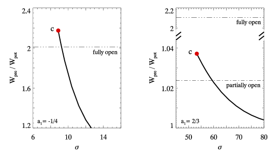
Figure 3: Left: The energy accumulation process before the catastrophe, $W_{\mathrm{pre}}/W_{\mathrm{pot}}$, in a background field with $a_{1}=-1/4$, along the stable branch as shown in Fig. 1. The fully open threshold is shown in dashed-three-dotted line. The accumulated magnetic energy goes beyond the fully open field threshold. Right: The energy accumulation before the catastrophe in a background field with $a_{1}=2/3$, along the stable branch as shown in Fig. 2. The fully open and partially open thresholds are shown in dashed-three-dotted and dashed-dotted lines, respectively. The accumulated magnetic energy goes beyond the partially open field threshold, but still lower than the the fully open field threshold.

The energy accumulation processes of the flux rope in the dipole dominated and multipole dominated background are shown in the left and right panel of Fig. 3, respectively. These two panels correspond to the energy accumulation processes before the catastrophic loss of equilibrium shown in Fig. 1 and Fig. 2, respectively. In this section we focus on the energy accumulation process in a dipole dominated background field shown in the left panel. Since there is only one closed flux system in the dipole dominated background for the case with $a_{1}=-1/4$, the opening up of closed background always induces fully open eruptions. Fully open magnetic fields can be obtained by flipping the boundary flux distributions in the southern hemisphere, i.e., $\mu\in[-1,0]$. A brief description of the procedures to obtain the field configuration and the energy threshold constrained by the fully open field is discussed in Appnedix A and B, respectively. The fully open energy threshold for the case of $a_{1}=-1/4$ is shown in dashed line in Fig. 3. We also present in this figure the normalized accumulated magnetic energy, $W_{\mathrm{pre}}/W_{\mathrm{pot}}$, versus the background flux, $\sigma$, before the catastrophe of flux ropes (in solid line). Note that the energy reaches maximum at the critical pre-eruptive point, marked by the red dot. Our calculations shows that the accumulated energy of the critical pre-eruptive state, $W_{\rm pre}(h_{c})/W_{\rm pot}$, is $2.17$. The energy threshold constrained by the fully open state, $W^{\rm f}_{\rm open}/W_{\rm pot}$, is $2.011$. The energy release fraction of the pre-eruptive magnetosphere, $[W_{\rm pre}(h_{c})-W^{\rm f}_{\rm open}]/W_{\rm pre}(h_{c})$, is about $7\%$. Observationally, the total magnetic energy in the magnetosphere is about $\sim 10^{46}({\rm B}/10^{14}G)^{2}(r_{s}/10{\rm km})^{3}$ergs, the giant flare is typically $10^{44}$ergs, so only $1\%$ of magnetic energy release in the magnetosphere could account for the giant flares (Woods & Thompson, 2006; Mereghetti, 2008). As a result, it is possible for the flux rope to fully open up the background field and provides abundant magnetic energy to drive a magnetar giant flare.

4.3 Partially Open Eruptions in Multipolar Backgrounds

In the previous section, we have established that for a dipole dominated background it is possible to induce fully open eruptions. However, observation shows that multipolar magnetic fields may be involved for magnetar giant flares (Feroci et al., 2001; Pavan et al., 2009). It is natural to know whether a fully open eruption is possible in the multipolar dominated background. We now investigate the energy accumulation process of the flux rope in multipole dominated background with $a_{1}=2/3$, the field configuration of which is also shown in Fig. 2. The detailed result is shown in the right panel of Fig. 3. The accumulated energy, $W_{\rm pre}(h_{c})/W_{\rm pot}$, in the critical pre-eruptive state is about $1.04$. However, energy threshold constrained by the fully open state, $W^{\rm f}_{\rm open}/W_{\rm pot}$, is $2.090$. It is clear that this flux rope eruption is impossible to fully open up the multipole dominated field.

However, it is interesting to note that the eruption may just involve partial opening up of the closed flux systems for multipole dominated background. It is conceivable that the partial opening up of the background field requires less work to be done than the full opening up of background field. This will reduce the energy threshold constrained by the full opening up eruption. Along this line we could find an alternative approach of the flux rope eruption. For this type of eruption, it may just involve partial opening up of the magnetic field, which has a lower threshold of $1.024$ (shown as dashed-dotted line in the right panel). It reduces the energy threshold constrained by fully open field. The critical pre-eruptive state contains energy about $1.5\%$ above the partially open threshold. The energy accumulation in the magnetosphere becomes sufficient to drive a partially open eruption.

4.4 Further Numerical Results

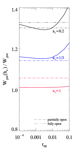
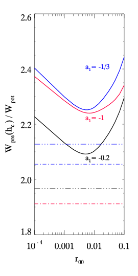
Figure 4: Left: Accumulated pre-eruptive magnetic energy as functions of $r_{00}$ for centrally-caved field with $a_{1}=0.2$ (black), $a_{1}=1/3$ (blue), and $a_{1}=1$ (red). The corresponding threshold values of partially open fields are shown in dashed-dotted lines in the same color. The corresponding threshold values of fully open fields are shown in dashed-three-dotted lines in the same color. Right: The same as left panel but for centrally-arcaded field with $a_{1}=-0.2$ (black), $-1/3$ (blue), and $-1$ (red).

Two representative examples are given in previous sections to show the flux rope eruption from the perspective of energy budget. Here we perform a comprehensive study on the flux rope energetics to check the possibility of the flux rope’s eruption in different kind of background field. We investigate the accumulated magnetic energy, $W_{\mathrm{pre}}(h_{c})/W_{\mathrm{pot}}$, for different values of $a_{1}\in[-1,1]$ and flux-rope radius $r_{00}\in[10^{-4},0.1]$. The results are shown in Fig. 4.

Let’s first focus on the cases with positive value of $a_{1}$, i.e., the cases with centrally-caved background field. In the left panel of this figure, the black solid line represents the accumulated energy $W_{\mathrm{pre}}(h_{c})/W_{\mathrm{pot}}$ in a centrally-caved multipolar field with $a_{1}=0.2$. Since the energy threshold of both the fully and partially open fields are relevant in the multipole dominated background, we show both the two energy thresholds in the same panel for comparison. The threshold value of the corresponding partially open field, $W_{\mathrm{open}}^{\mathrm{p}}/W_{\mathrm{pot}}$, and the fully open field, $W_{\mathrm{open}}^{\mathrm{f}}/W_{\mathrm{pot}}$, are shown respectively in black dashed-dotted line and black dashed-three-dotted line. Detailed calculation of the two energy thresholds is given in Appendix A and B. It can be found that, when $r_{00}\lesssim 0.0007$ or $r_{00}\gtrsim 0.01$, the accumulated pre-eruptive energy could surpass the partially open threshold. And when flux rope’s minor radius is larger, i.e., with $r_{00}\gtrsim 0.02$, the accumulated pre-eruptive energy could even surpass the fully open threshold. We also show the comparison of the accumulated pre-eruptive energy (shown in blue solid line) in a centrally-caved background field for the stronger multipolar component $a_{1}=1/3$ with the relevant energy threshold. The corresponding partially open threshold is shown in the blue dashed-dotted line. It can be found that, for all possible value of $r_{00}$, the accumulated pre-eruptive energy is higher than the partially open threshold. However, none of them could surpass the fully open threshold $\sim 1.49$, which is beyond the scale of this figure and not shown. We choose $a_{1}=1$ to represent a centrally-caved background field with much stronger multipolar component. The dependence of the accumulated pre-eruptive energy on the flux rope minor radius for $a_{1}=1$ is shown as red solid line. It is obvious that for all possible value of $r_{00}$, the flux rope cannot accumulate enough energy to surpass the corresponding partially open threshold, shown as the red dashed-dotted line. Since the fully open threshold is always higher than the partially open threshold, the flux rope could not support fully open eruption either in this case. It is clear that for centrally-caved multipole dominated field, if the multipole components are too strong, the flux rope is not able to erupt.

Now let’s turn to the centrally-arcaded background fields, i.e., the cases with the multipole parameter $a_{1}$ of negative sign. The black solid line in the right panel of Fig 4 represents the accumulated pre-eruptive energy in a dipole dominated field with $a_{1}=-0.2$. For the dipole dominated background, the relevant energy threshold is only constrained by fully open field and this threshold is shown in black dashed-three-dotted line in this figure. It is obvious that, for all possible value of $r_{00}$, the flux rope could build up more magnetic energy before the catastrophe and give rise to fully open eruptions in the dipole dominated background. The blue solid line in this figure represents the accumulated pre-eruptive magnetic energy in a centrally-arcaded multipolar field with $a_{1}=-1/3$. In this case, the relevant thresholds are restricted by either the fully or the partially open field. Detailed calculation shows that the pre-eruptive energy could surpass both the corresponding partially open threshold, shown in blue dashed-dotted line, and the fully open threshold, shown in blue dashed-three-dotted line. The red solid line represents the variation of the accumulated energy with the flux rope’s minor radius in a background field with $a_{1}=-1$, i.e., a centrally-arcaded field with stronger multipolar component. The pre-eruptive energy could surpass the corresponding partially open threshold, shown in dashed-dotted red line. However, the flux rope could not accumulate enough energy to get over the corresponding fully open threshold ($\sim 2.89$, not shown in this figure).

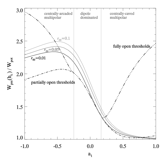
Figure 5: Accumulated pre-eruptive magnetic energy as functions of $a_{1}$ with $r_{00}=0.01$ (black), $0.05$ (grey), and $0.1$ (light grey). The corresponding threshold values of partially-open fields and fully-open fields are shown in dashed-dotted line and dashed-three-dotted line, respectively. Two vertical lines represent the separatrix between the dipole-dominated fields and the multipole-dominated fields.

Our prior results show that the possibility of the flux rope’s eruption depends on the parameter $a_{1}$ in a rather complex way. These complex behavior can be more readily comprehensible in Fig. 5. We show in this figure the dependence of accumulated pre-eruptive magnetic energy on the parameter $a_{1}$ for different fixed value of $r_{00}$. The relevant energy thresholds of fully and partially open fields are shown as well in dashed-three-dotted and dashed-dotted line, respectively. The comparison of the accumulated pre-eruptive energy and the energy thresholds can be made in a more straightforward way. The solid black, grey, and light grey lines represent the accumulated pre-eruptive magnetic energy for typical flux rope minor radius $r_{00}=0.01$, $0.05$, and $0.1$, respectively. Note that partially open thresholds do not exit in dipole dominated fields with $a_{1}\in[-1/4,1/6]$, which is shown as two vertical lines in this figure.

We found that, in the dipole dominated background fields, i.e., $a_{1}\in[-1/4,1/6]$, it is always possible to drive a fully open eruption. However, in most cases of the multipole background fields, the fully open energy threshold is always greater than the energy stored in the critical pre-eruptive state and it is impossible for the flux rope to induce fully open eruptions. Only in some special cases, when the multipole components are not so strong , i.e., $-0.55\lesssim a_{1}\lesssim-0.25$ or $1/6\lesssim a_{1}\lesssim 0.25$, it is possible to induce fully open eruptions.

More importantly, we note that in these fields, the eruption may just involve partially opening up of the close the magnetic flux, which provides an alternative approach for the flux rope eruptions. It is clearly discernable in this figure that, the energy release fraction, $\left[W_{\rm pre}(h_{c})-W^{\rm p}_{\rm open}\right]/W_{\rm pre}(h_{c})$, is about $10\%\sim 25\%$ during the partially open eruptions in the centrally-arcaded backgrounds, which is able to release and drive the giant flares. The energy release fraction for flux ropes embedded in the centrally-caved backgrounds is in a smaller range, within $\sim 5\%$. Note that there exits a special class of background fields with very strong centrally-caved multipole component, $a_{1}\gtrsim 0.75$. The pre-eruptive energy possessed in flux ropes is always lower than the partially open thresholds. These kind of background fields cannot be opened up by eruptions of flux ropes.

Note in addition that the simplest case of $a_{1}=0$ has been investigated by Lin et al. (1998). However, their approximate treatment of the flux frozen constraints has led them to the inappropriate result that the flux rope can not support the fully open eruption. In our paper, we rigorously take into account the flux-frozen constraint and come to the different results with theirs.

5 Conclusions and Discussions

We propose a force-free magnetospheric model with an embedded helically twisted flux rope. With the gradual variations at the magnetar surface, the flux rope evolves quasi-statically in stable equilibrium states. Upon the loss of equilibrium point is reached, the global magnetospher is then destabilized and the flux rope erupts catastrophically. During the process, the original closed flux systems would be opened up, accompanied by rapid release of the magnetic energy stored in magnetosphere. This energy release is of vital importance for the outbursts of magnetars. However, the feasibility that the flux systems’ opening-up could be achieved depends on whether the amount of energy accumulated prior to the flux rope eruptions could surpass the energy thresholds constrained by the post-eruptive open magnetic topologies.

In this paper, we adopt boundary conditions, which include both the contribution from a dipolar component and a high order multipolar component, to illustrate the complicated geometry of magnetic field close to magnetar surface. We establish fully open field for the dipole dominated magnetic fields, which involves the opening up the single closed flux system in the backgrounds. For multipole dominated closed background, we establish the partially open field, which involves opening up of part of the closed flux systems, as well as the fully open field, which involves opening up of all closed flux systems. The opening up of closed magnetic fields requires certain amount of work to be done to overcome the attractive magnetic tension force. Since partially open fields require less closed flux systems to be opened up, the energy thresholds constrained by the partially open fields is lower than those by the fully open fields. Both the field configuration and the magnetic energy threshold of the two kinds of open field are examined. Then we carefully investigate the magnetic energy accumulation process before the catastrophe, especially the magnetic energy stored at the critical catastrophic point.

We find that it is possible to fully open up dipole dominated background fields for catastrophic eruptions of flux ropes. However, it is generally difficult to fully open up multipole dominated background fields. In most cases with multipole dominated backgrounds, the magnetic energy stored at critical pre-eruptive point is significantly lower than the fully open thresholds, which suggests that the flux rope can not support fully open eruptions. Fortunately, we find that the accumulated magnetic energy at the critical point is higher than the partially open thresholds. This provides an alternative opportunity for the flux rope to erupt in the multipolar magnetosphere. The multipole dominated fields can be either centrally-caved or centrally-arcaded, depending on the flux profiles on the magnetar surface. Generally speaking, the magnetic energy stored in critical pre-eruptive magnetosphere surpasses the partially open energy threshold about $10\%\sim 25\%$, if the flux rope is initially embedded in a centrally-arcaded background field. For a flux rope initially embedded in a centrally-caved background field, the magnetic energy stored in critical pre-eruptive magnetosphere could surpass the partially open threshold, if the multipolar component is mildly strong, i.e., $1/6<a_{1}\lesssim 0.75$. The energy release fraction is within $\sim 5\%$. If the multipolar component becomes even stronger, $a_{1}\gtrsim 0.75$, the accumulated magnetic energy cannot go beyond the partially open threshold and the partially open eruption of flux rope in not possible.

The magnetic energy of the critical pre-eruptive state in excess of the fully or partially open threshold is assumed to be released in fast dynamical timescale. Observationally, the total magnetic energy in the magnetosphere is about $\sim 10^{46}({\rm B}/10^{14}G)^{2}(r_{s}/10{\rm km})^{3}$ergs, the giant flare is typically $10^{44}$ergs, so only $1\%$ of magnetic energy release in the magnetosphere could account for the giant flares. Theoretically, all cases with surplus energy fraction larger than $1\%$ are possible to drive magnetar giant flares. Specifically for boundary conditions adopted in this paper, most cases with $-1\leq a_{1}\lesssim 0.75$ are possible to drive magnetar giant flares.

In addition to the physical processes considered in this paper, the magnetic field can also be opened up by the strong neutron star wind (Bucciantini et al. 2006). If the field lines are opened up by the neutron star wind at a larger distance from the neutron star, the amount of open magnetic flux would be reduced, and the magnetic energy to support the eruption would also decrease. To study how the neutron star wind affects the flux rope eruption energetics, we need to establish a model with a current sheet in the magnetosphere. Currently, we are now trying to construct a magnetosphere model to account for this important process. We leave the investigation about the situations with current sheet formation in a companion paper (Huang & Yu, in prep).

Figure 1: Left: Equilibrium curve of the flux rope in a dipole-dominated background with $a_{1}=-1/4$ and $r_{00}=0.01$, which shows the dependence of the height of the flux rope on the magnetic flux at the magnetar surface. The magnetospheric field configuration . The lower stable branch and the upper unstable branch are shown in solid line and dotted line, respectively. The red dot marks the critical point. Right: Magnetosphere with an embedded flux rope in the pre-eruptive critical state. The thick solid semi-circle represents the magnetar surface. The dashed line represents a circle with a radius of the critical height of the flux rope $h_{c}$.

Appendix A Configurations of Partially Open and Fully Open Magnetic Fields

In this appendix, we describe procedures to get the fully open magnetic field from dipole dominated field, and to get both fully and partially open field from multipole dominated field. We show three illustrative examples in Fig. 6.

In the upper row we show a dipolar field with $a_{1}=0$, as an example of dipole dominated fields with $a_{1}\in[-1/4,1/6]$. The configuration of potential background field is shown in top-left panel. The thick solid semi-circle in these figures represents the magnetar surface. To be clear, we show the boundary flux distribution in solid line in the sub-panel. Only one extremum appears in boundary flux distribution. The fully open field is obtained by simply flipping the surface flux distribution of the potential field in the southern hemisphere, i.e., $-1\leq\mu<0$ or $\pi/2<\theta\leq\pi$. The configuration of the fully open field is shown in top-middle panel. The corresponding boundary flux distribution is shown in dashed-three-dotted line in the sub-panel. The boundary flux distribution of the original closed field is also shown in solid grey line for comparison.

There would appear three extremum points in the boundary flux distribution for parameters $a_{1}\in[-1,-1/4)$ or $a_{1}\in(1/6,1]$, so that multipolar configurations arise in the background magnetic field. Under these circumstances, two kinds of open field configurations, i.e., partially open and fully open fields, can be obtained. The middle row is for a centrally-caved field with $a_{1}=1$ and the lower row is for a centrally-arcaded field with $a_{1}=-1$. Configurations of potential background fields, partially open fields, and fully open fields are shown in the left, middle and right panels, respectively. In the following we describe the mathematical manipulations to obtain these two kinds of open fields of the case $a_{1}=1$ as an example. The case of $a_{1}=-1$ can be obtained in a similar way.

The partially open field is obtained by simply flipping the surface flux distribution of the potential field in the southern hemisphere. The corresponding boundary flux distribution is shown in dashed-dotted line in the sub-panel of middle-middle panel. It can be readily identified that only field lines near the central extremum around $\mu=0$ are opened up, while the other two closed flux systems around the nonzero extremum points remain closed. In this sense, we call the resulting magnetic field configurations as partially open fields. The fully open field configurations can be obtained from original potential field in two steps. The details are clearly illustrated in the sub-panel of the middle-right panel. In the first step, the boundary flux between the two nonzero extremum points are reversed. After this step, the modified boundary flux contains only one extremum point at $\mu=0$ (see the dashed line in the subpanel). In the second step, the southern hemisphere boundary flux are flipped and the resulting boundary flux distribution is shown as the dashed-three-dots line. The closed configurations of the patterns caused by the high order multipolar terms are also opened up, shown in thick black lines near two poles of magnetar. There are three current sheets in total in fully open field, together with the equatorial one.

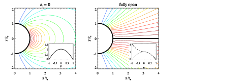
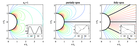
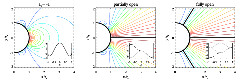
Figure 6: Top-Left: Configuration of a dipolar field. The boundary flux distribution is shown as solid line in the sub-panel. Top-Middle: Configuration of the corresponding fully open field. The thick solid line on the equatorial plane represents the current sheet formed by the opening up of the single closed flux system of the background. The boundary flux distribution is obtained by flipping the surface flux distribution of the potential field and is shown as dashed-dotted line in the sub-panel. Middle-Left: Configuration of a centrally-caved potential field with $a_{1}=1$. Middle-Middle: Configuration of partially open field with $a_{1}=1$. The thick solid line on the equatorial plane represents the current sheet formed by the opening up of the central closed flux system. Midle-Right: Configuration of fully open field with $a_{1}=1$, with three current sheets formed by the opening up of all the three closed flux systems in the background, shown in thick solid lines. The boundary flux distribution is also obtained based on the surface flux distribution of the potential field and is shown as dashed-three-dotted line in the sub-panel. Bottom-left: Configuration for a centrally-arcaded potential field with $a_{1}=-1$. Bottom-Middle : partially open field with $a_{1}=-1$. Bottom-Right: fully open field with $a_{1}=-1$.

Appendix B Energy of Partially Open and Fully Open Magnetic Fields

The boundary condition of the post-eruptive partially open field is obtained by flipping the flux function according to the original boundary condition of the closed potential field (Yu, 2011). Explicitly, the modified boundary flux distribution of the partially open field can be written as (see the sub-panels of partially open fields shown in Fig. 6)

$$\Theta^{\rm p}_{\rm open} = \left\{\begin{array}[]{cc}\Theta(\mu),&0\leq\mu\leq 1\\ 2\Theta(0)-\Theta(\mu),&-1\leq\mu\leq 0\ ,\end{array}\right.$$ (B3)

where $\Theta(\mu)$ is already defined in Equation (6). The general solutions to the GS equation are of the form

$$\Psi^{\mathrm{p}}_{\mathrm{open}}(r,\mu) = \Psi(r_{s},0)(1-\mu)+\sum_{k=1}^{\infty}a_{2k}r^{2k+1}\ \left[\frac{P_{2k-1}(\mu)-P_{2k+1}(\mu)}{4k+1}\right]\ .$$ (B4)

To determine the partially open field, we have to specify the coefficients $a_{2k}$’s in the above equation. For convenience, we define the following flux function as

$$\Phi(r,\mu) = \Psi^{\mathrm{p}}_{\mathrm{open}}(r,\mu)\ -\ \Psi(r_{s},0)(1-\mu)$$ (B5)

$$= \sum_{k=1}^{\infty}a_{2k}r^{2k+1}\ \left[\frac{P_{2k-1}(\mu)-P_{2k+1}(\mu)}{4k+1}\right].$$

According to the orthogonality of associated Legendre polynomials $P_{2k}^{1}(\mu)$ and $\Psi(r_{s},\mu)=\Psi_{0}\sigma\Theta(\mu)$, we can determine the coefficients $a_{2k}$ as

$$a_{2k} = \frac{4k+1}{r_{s}^{2k+1}}\ \int_{0}^{1}\Phi(r_{s},\mu)\ P_{2k}^{1}(\mu)\ d\mu$$ (B6)

$$= \Psi_{0}\sigma\ \frac{4k+1}{r_{s}^{2k+1}}\ \int_{0}^{1}\left[\Theta(\mu)-\Theta(0)(1-\mu)\right]\ P_{2k}^{1}(\mu)\ d\mu\ .$$

Once these coefficients are fixed, we can get the the partially field configurations.

The boundary condition of the post-eruptive fully open field is obtained in a similar way to the partially open field. The difference is that we also need to flip the original boundary flux profile in the range $[0,1]$. Hereafter we use $\Theta^{*}(\mu)$ to denote the flipped boundary flux profile in the range $[0,1]$. The modified boundary flux profile in the entire range $[-1,1]$ can be expressed in terms of $\Theta^{*}(\mu)$ as (see the sub-panels of fully open fields shown in Fig. 6)

$$\Theta^{\rm f}_{\rm open} = \left\{\begin{array}[]{cc}\Theta^{*}(\mu),&0\leq\mu\leq 1\\ 2\Theta^{*}(0)-\Theta^{*}(\mu),&-1\leq\mu\leq 0\ .\end{array}\right.$$ (B9)

where the new surface flux distribution $\Theta^{*}(\mu)$ in the range $[0,1]$ is flipped as follows,

$$\Theta^{*}(\mu) = \left\{\begin{array}[]{cc}\Theta(\mu)\ ,&\mu_{1}\leq|\mu|\leq 1\\ (4a_{1}+1)^{2}/(10a_{1})\ -\ \Theta(\mu)\ ,&0\leq|\mu|<\mu_{1}\\ \end{array}\right.\ ,$$ (B12)

where $\mu_{1}=\sqrt{(6a_{1}-1)/(10a_{1})}$ is the nonzero extremum point in the range $[0,1]$. Similarly, we can determine the coefficients $a_{2k}$’s in Equation (B4) in terms of the surface flux distribution of the fully open field, $\Theta^{\rm f}_{\rm open}$. The fully open field subsequently can be determined in complete detail.

The magnetic energy possessed in the post-eruptive state, $W_{\mathrm{open}}^{\mathrm{p}}$ for partially-open fields state or $W_{\mathrm{open}}^{\mathrm{f}}$ for fully-open fields state in this paper, reads

$$W^{\rm p,f}_{\mathrm{open}} = \int\frac{{{\bf B}_{\rm open}^{\rm p,f}}^{2}}{8\pi}\ dV=\int_{\partial V}\frac{\left(B_{\rm open}^{\rm p,f}\right)^{2}}{8\pi}({\bf r}\cdot d{\bf S})-\frac{1}{4\pi}\int_{\partial V}({\bf B}_{\rm open}^{\rm p,f}\cdot{\bf r})({\bf B}_{\rm open}^{\rm p,f}\cdot d{\bf S})\ ,$$ (B13)

according to magnetic virial theorem. The energy thresholds in fully-open fields and partially-open fields are calculated by $W_{\mathrm{open}}^{\mathrm{f}}/W_{\mathrm{pot}}$ and $W_{\mathrm{open}}^{\mathrm{p}}/W_{\mathrm{pot}}$, respectively.

References

- Aly (1984) Aly, J. J., 1984, ApJ, 283, 349
- Aly (1991) Aly, J. J., 1991, ApJ, 375, L61
- Antiochos et al. (1999) Antiochos, S. K., DeVore, C. R., & Klimchuk, J. A., 1999, ApJ, 510, 485
- Beloborodov (2009) Beloborodov, A. M., 2009, ApJ, 703, 1044
- Bucciantini et al. (2006) Bucciantini, N., Thompson, T. A., Arons, J., Quataert, E., & Del Zanna, L., 2006, MNRAS, 368, 1717
- Chandrasekhar (1961) Chandrasekhar, S, 1961, Hydrodynamic and Hydromagnetic Stability (Oxford: Oxford Univ. Press)
- Duncan & Thompson (1992) Duncan, R. C., & Thompson, C., 1992, ApJ, 392, L9
- Feroci et al. (2001) Feroci, M., Hurley, K., Duncan, R. C., & Thompson, C., 2001, ApJ, 549, 1021
- Forbes & Priest (1995) Forbes, T. G. & Priest, E. R. 1995, ApJ, 446, 377
- Forbes (2010) Forbes, T. G., 2010, in Heliophysics: Space Storms and Radiation: Causes and Effects, ed. J. S. Carolus & L. S. George (Cambridge: Cambridge Univ. Press), 159
- Gaensler et al. (2005) Gaensler, B. M., Kouveliotou, C., & Gelfand, J. D. 2005, Nature, 434, 1104
- Gavriil et al. (2002) Gavriil, F. P., Kaspi, V. M., Woods, P. M. 2002, Nature, 419, 142
- Gill & Heyl (2010) Gill, R., & Heyl, J. S. 2010, MNRAS, 407, 1926
- Götz et al. (2007) Götz, D., Mereghetti, S., & Hurley, K. 2007, Ap&SS, 308, 51
- Huang & Yu (in prep) Huang, L. & Yu, C., in preparation
- Hurley et al. (2005) Hurley, F., et al. 2005, Nature, 434, 1098
- Jones (2003) Jones, P. B. 2003, ApJ, 595, 342
- Kluźniak & Ruderman (1998) Kluźniak, W. & Ruderman, M., 1998, ApJ, 505, L113
- Kouveliotou et al. (1998) Kouveliotou, C., et al. 1998, Nature, 393, 235
- Levin & Lyutikov (2012) Levin, Y., & Lyutikov, M. 2012, MNRAS, 427, 1574L
- Lin et al. (1998) Lin, J., Forbes, T. G., Isenberg, P. A., & Démoulin, P. 1998, ApJ, 504, 1006
- Lundquist (1950) Lundquist, S. 1950, Ark. Fys., 2, 361
- Lyutikov (2006) Lyutikov, M. 2006, MNRAS, 367, 1602
- Lyutikov (2013) Lyutikov, M. 2013, arXiv: 1036.2264
- Mazets et al. (1979) Mazets, E. P., et al. 1979, Nature, 282, 587
- Mereghetti (2008) Mereghetti, S. 2008, A&AR, 15, 225
- Mereghetti (2013) Mereghetti, S. 2013, in Proc. 26th Texas Symp. on Relativistic Astrophysics (arXiv: 1304.4825)
- Mereghetti & Stella (1995) Mereghetti, S. & Stella, L. 1995, ApJ, 442, L17
- Palmer et al. (2005) Palmer, D. M., et al. 2005, Nature, 434, 1107
- Parfrey et al. (2013) Parfrey, K., Beloborodov, A. M., Hui, L., 2013, ApJ, 774, 92
- Pavan et al. (2009) Pavan, L., Turolla, R., Zane, S., & Nobili, L. 2009, MNRAS, 395, 753
- Perna & Gotthelf (2008) Perna, R. & Gotthelf, E. V. 2008, ApJ, 681, 522
- Priest & Forbes (2000) Priest E., & Forbes T. 2000, Magnetic Reconnection. MHD Theory and Applications. Cambridge Univ. Press, Cambridge
- Ruderman (1991) Ruderman, M. 1991, ApJ, 366, 261
- Shafranov (1966) Shafranov, V. D. 1966, Rev. Plasma Phys., 2, 103
- Sturrock (1991) Sturrock, P. A. 1991, ApJ, 380, 655
- Thompson et al. (2002) Thompson, C., Lyutikov, M., & Kulkarni, S. R. 2002, ApJ, 574, 332
- Wood et al. (2001) Woods, P. M. et al. 2001, ApJ, 552, 748
- Woods & Thompson (2006) Woods, P. M., & Thompson, C., 2006, in Compact Stellar X-Ray Sources, ed. W. H. G. Lewin & van der Klis (Cambridge Univ. Press), 547
- Woods et al. (2007) Woods, P. M., Kouveliotou, C., Finger, M. H., et al. 2007, ApJ, 654, 470
- Yu (2011) Yu, C., 2011, ApJ, 738, 75
- Yu (2012) Yu, C., 2012, ApJ, 757, 67
- Yu & Huang (2013) Yu, C. & Huang, L., 2013, ApJ, 771, L46
- Zhang & Low (2001) Zhang, M., & Low, B. C., 2001, ApJ, 561, 406