1-D and 2-D Parallel Algorithms for All-Pairs Similarity Problem

Abstract

All-pairs similarity problem asks to find all vector pairs in a set of vectors the similarities of which surpass a given similarity threshold, and it is a computational kernel in data mining and information retrieval for several tasks. We investigate the parallelization of a recent fast sequential algorithm. We propose effective 1-D and 2-D data distribution strategies that preserve the essential optimizations in the fast algorithm. 1-D parallel algorithms distribute either dimensions or vectors, whereas the 2-D parallel algorithm distributes data both ways. Additional contributions to the 1-D vertical distribution include a local pruning strategy to reduce the number of candidates, a recursive pruning algorithm, and block processing to reduce imbalance. The parallel algorithms were programmed in OCaml which affords much convenience. Our experiments indicate that the performance depends on the dataset, therefore a variety of parallelizations is useful.

1 Introduction

Given a set $V$ of $m$-dimensional $n$ vectors and a similarity threshold $t$, the all-pairs similarity problem asks to find all vector pairs with a similarity of $t$ and more. Given the high dimensionality of many real-world problems, such as those arising in data mining and information-retrieval, this task has proven itself to be quite costly in practice, as we are forced to use the brute-force algorithms that have a quadratic running time complexity. Recently, Bayardo et. al [8] have developed time and memory optimizations to the brute force algorithm of calculating the similarity of each pair in $V\times V$ and filtering them according to whether the similarity exceeds $t$. We may assume the vectors are in $R^{m}$ and the similarity function is inner product without much loss of generality.

Two 1-D data distributions are considered: by dimensions (vertical) and by vectors (horizontal). We introduce useful parallelizations for both cases. We have observed that the optimized serial algorithms are suitable for parallelization in this fashion, thus we have designed our algorithms based upon the fastest such algorithm. It turns out that our horizontal algorithms especially attain a good amount of speedup, while the elaborate vertical algorithms can attain a more limited speedup, partially due to limitations in our implementation. Additional contributions to the 1-D vertical distribution include a local pruning strategy to reduce the number of candidates, a recursive pruning algorithm, and block processing to reduce imbalance. We have combined the two data distribution strategies to obtain an elegant 2-D parallel algorithm. We also take a look at the performance of a previously proposed family of optimized sequential algorithms and determine which of those optimizations may be beneficial for a distributed memory parallel algorithm design. We have implemented the parallel algorithms in the functional language OCaml. A performance study compares the performance of the proposed algorithms on small and large real-world datasets.

1.1 Overview

The rest of the paper is organized as follows. Section 2 briefly gives the background of the problem while in Section 3 we review related work. Optimizations to the sequential algorithm are covered in Section 4. Section 5 introduces the 1-D vertical and horizontal parallelizations, and likewise Section 6 presents the 2-D parallelization. Section 7 contains the performance study and Section 8 explains our conclusions and future work.

1.2 Contributions

Upon the first author’s suggestion that two-dimensional algorithms would be appropriate for frequent itemset mining and text categorization problems, the second author contributed the idea that a two-dimensional algorithm could work for the Euclidian all-pairs similarity problem (which the first author suggested as an important problem as input to graph transduction algorithms), and offered a parallelization based on a mesh network. The first author later refined that approach by designing algorithms that parallelize the recent fast all-pairs similarity algorithms developed at Google. The first author then optimized the algorithms for non-blocking networks, including the pruning and vector blocking approaches. The first author proved the theorems, made the implementation in OCaml, performed the experiments, and wrote the paper. The second author was the PhD supervisor of the first author at the time of writing, and guided the research by making valuable suggestions, and has endorsed this paper. The second author also carefully reviewed and guided all theoretical research on this problem and contributed the performance analysis framework in Section 7, which the first author extended.

2 Background

2.1 Problem definition

Let $V=\{v_{1},v_{2},v_{3},...,v_{n}\}$ be the set of sparse input vectors in $R^{m}$, following a similar terminology to [8]. Let $t$ be the similarity threshold. Let a sparse vector $x$ be made up of $m$ components $x[i]$, where some $x[i]=0$; such a sparse vector can be represented by a list of pairs $\left[(i,x[i])\right]$ in which only non-zero components are stored. Let $|x|$ be the number of non-zero components in the vector, that is the length of its list representation. Let $||x||$ be the vector’s magnitude. Let also $size(V)=\sum_{v\in V}|v|$ be the number of non-zero values in $V$. Each vector $v_{i}$ is made up of components per dimension $d$, where the vector’s $d$th component is denoted as $v_{i}[d]$. The similarity function is defined as the summation of input values from similarity among individual components: $sim(x,y)=\sum_{i}sim(x[i],y[i])$. Another accumulation function instead of summation may be used (for instance any other binary operation which has the same algebraic properties), however summation is enough for many purposes. The problem is to find the set of all matches $M=\{(v_{i},v_{j})\ |\ {v_{i}\in V}\land{v_{i}\in V}\land{i\neq j}\land{sim(v_{i},v_{j})\geq t}\}$.

Without much loss of generality, we assume that input vectors are normalized (for all $x\in V,||x||=1$), and for vectors $x$ and $y$, $sim(x,y)$ function is the dot-product function $dot(x,y)=\sum_{i}x[i].y[i]$, that is $sim(x[i],y[i])=x[i].y[i]$. The algorithms can be easily generalized to other similarity functions which are composed from similarities $sim(x[i],y[i])$ across individual dimensions.

The input dataset $V$ may also be interpreted as a data matrix $D$ where row $i$ is vector $v_{i}$. In this case, we may represent similarities by the similarity matrix $S=D.D^{T}$ where $S_{ij}=dot(v_{i},v_{j})$ obviously, and we find the set of matches $M=\{(i,j)\ |\ S_{ij}\geq t\}$. More naturally, we may interpret the output as a match matrix $M$ that is defined as:

$$M^{\prime}_{ij}=\begin{cases}0&\text{if}\ S_{ij}<t,\\ S_{ij}&\text{if}\ S_{ij}\geq t\end{cases}$$ (1)

The output set of matches $M$ may be considered to define an undirected similarity graph $G_{S}(V,t)=(V,M)$. In this case an edge $u\leftrightarrow v$ denotes a similarity relation between vectors $u$ and $v$; the edge weight $w(u,v)=u.v$.

2.2 Applications

An all pairs similarity algorithm may be viewed as a computational kernel for several tasks in data mining and information retrieval domains. In data mining and machine learning, the similarity graph may be supplied as input to efficient graph transduction [27, 43], graph clustering algorithms [9] and near-duplicate detection (by using a high threshold to filter edges). Obviously, once a similarity graph is computed, classical k-means [34, 33] or k-nn algorithms [22, 19], which are widely used in data mining due to their effectiveness in low number of dimensions, may be adapted to use the graph instead of making the geometric calculations directly over input vectors. As frequent itemset mining may be viewed as the costly phase of association rule mining class of algorithms; likewise, the graph similarity problem may be viewed as the costly phase of several classification, transduction, and clustering algorithms.

Calculating the similarity graph may be alternately viewed as capturing the essential geometry of (the similarities in) the dataset, on which any number of computational geometry algorithms may be run. This is basically what a classification or clustering algorithm does given similarities in the data: the algorithm tries to find geometric distinctions, either determining a class boundary for classification, or identification of clusters by grouping similar points according to the similarity geometry. Note also that with an adequate similarity threshold, we can obtain a connected graph and therefore approximate all similarities in the dataset.

Constructing the similarity graph also has the unique advantage in that it can be re-used later for additional data mining tasks. For instance, one application can make a hierarchical clustering of the data, and another one can use it for transduction. Basically, we think that any data mining task that has a geometric interpretation can use the similarity graph as input successfully. Therefore, we anticipate that the parallel similarity graph construction will be a staple of future parallel data mining systems.

3 Related Work

3.1 k-nearest neighbors problem

The problem of constructing a similarity graph can be contrasted with k-nearest neighbors problem, which is a slightly harder problem but can be solved approximately using a distance threshold. Our use of the dot-product between two vectors should not be misleading either, as that corresponds to range search in a corresponding metric space, to emphasize the close relation between these problems. At any rate, some of the same approaches can be adapted to similarity graph construction, therefore we should take them into account. Especially, note that most of the difficulties with nearest neighbor search carry over to our problem.

Due to the curse of dimensionality [36], the brute-force algorithm of nearest neighbor search is quite difficult to improve upon [44]. In practice, there are no advanced geometric data structures that will give us algorithmic shortcuts [15, 6]. In the general setting of metric spaces, the nearest neighbor problem is non-trivial and data structures are not very effective for high dimensionality [18]. This implies that we cannot rely on space partitioning or metric data structures that work well in low number of dimensions, although of course, non-trivial extensions of those methods may prove to be effective such as combining dimensionality reduction with geometric data structures.

3.2 Related sequential algorithms

3.2.1 Sequential knn algorithms

Some popular approaches to solving the nearest neighbor problem may be summarized as geometric data structures such as R-Tree[24]; VP-Tree [45], GNAT [10] and M-Tree [17] for general metric spaces, pivot-based algorithms [21, 12], random projections for $\epsilon$-approximate solutions to the knn problem [28], combining random projections and rank aggregation for approximation [20], locally sensitive hashing [23, 1, 3], and other data structures and algorithms for approximations [30, 5]. An algorithm related to our area of interest detects duplicates by using an inverted index [26]. Space-filling curves have also been applied to the knn problem [40, 31, 35].

Space-partitioning approaches usually do not work well for very high-dimensional data due to the curse of dimensionality, a thorough treatment of which is available in [44]. Weber et. al quantify in that article lower bounds on the average performance of nerarest neighbor search for space and data partitioning assuming uniformly distributed points, which show that for space partitioning like k-d trees, the expected NN-distance grows with increasing dimensionality, rendering such methods ineffective for high-dimensional data (full scan needed when $d>60$), and for data-partitioning the number of blocks that have to be inspected increase rapidly with increasing number of dimensions, for both rectangular (full scan is faster when $d>26$) and spherical bounding regions (full scan when $d>45$), and they also generalize their results to any clustering scheme that uses convex clusters, not just these. Their conclusion is that in high-dimensional data, the partitioning methods all degenerate to sequential search, in uniformly distributed data. We emphasize that their results imply that trivial geometric partitions of the data using hyperplanes or hyperspheres are mostly ineffective in very high-dimensional data, although they can in some cases work well for datasets with limited dimensionality or different distribution. Weber et. al for this reason propose the VA-file, which approximates vectors using bitstrings [44] and improves upon sequential scan.

In general, it seems that for solving proximity problems exactly in very high-dimensional datasets, techniques that prune candidates work well. Kulkarni and Orlandic, on the contrary, successfully use a data clustering method to optimize knn search in databases, which the authors show to be better than sequential scan and VA-file up to 100 dimensions on random datasets and 56 dimensions on real-world datasets [29], although it is impossible to know the true efficiency of these algorithms proposed by database researchers unless they are compared to fast in-memory algorithms since disk access time dominates the running time of algorithms that work on secondary storage. Also, such approaches do not usually scale up to very high number of dimensions.

Note that there are asymptotically optimal nearest neighbor algorithms in the literature. Vaidya introduces an asymptotically optimal algorithm for the all nearest neighbors problem which has $O(n\log n)$ time complexity [41]. The same algorithm solves $k$-nearest neighbors problem in $O(n\log n+kn\log k)$ time, while Callahan and Korasaraju propose an optimal $k$ nearest neighbors algorithm which runs in $O(n\log n+kn)$ time [13]. It is not immediately obvious why there are no experiments measuring the real-world performance of these optimal algorithms, however, it is conceivable that they may not have been practical for high-dimensional datasets, or it may have been considered that they require large constant factors.

We refer the reader to Chavez’s survey of search methods in metric spaces [16] for more information on the myriad algorithms. Chavez identifies three kinds of search algorithms for metric spaces: pivot-based algorithms, range coarsening algorithms, and compact partitioning algorithms, and he emphasizes that the search time of exact algorithms grow with intrinsic dimensionality of the metric space, which also increases the search radius, and thus makes it harder to compete with brute-force algorithms. As we have seen, similar problems also plague search algorithms in Euclidian spaces. For these reasons, researchers in recent years have turned to practical optimizations over brute-force algorithms, which we shall now examine briefly with a good example.

3.2.2 Practical sequential similarity search

In Bayardo et. al [8], the authors propose three main algorithms which embody a number of heuristic improvements over the quadratic brute force all-pairs similarity algorithm. These algorithms are summarized below. In the algorithms, each vector $x$ has components with weights $x[i]$, there are $m$ dimenions (or features) numbered from $1$ to $m$, $maxweight_{i}(V)$ is the maximum weight in dimension $i$ of the entire dataset $V$, and $maxweight(x)$ is the maximum weight in a vector $x$, following the notation in their paper.

all-pairs-0

This is equivalent to the brute force algorithm, with the additional on-the-fly construction of an inverted index as each vector is matched and indexed in turn. The calculation of the dot-product scores are achieved by consulting the inverted index. Thus each vector is compared to all the previous vectors that have been indexed, and then the vector itself is added to the index. This algorithm is thus slower than the brute force algorithm. In the matching of a new vector $x$, the algorithm uses a hash table $A$ to store the weights of candidates to match against $x$, since the vectors are sparse. The pseudocode for all-pairs-0 is given in Algorithm 1 and Algorithm 2.

Algorithm 1 $\textsc{All-Pairs-0}(V,t)$

  $M\leftarrow\emptyset$

  $I\leftarrow\textsc{Make-Sparse-Matrix}(m,n)$

  for all $v_{i}\in V$ do

        $M\leftarrow M\cup\textsc{Find-Matches-0}(v_{i},I,t)$

        for all $v_{i}[j]$ where $v_{i}[j]>0$ do

              $I_{ji}\leftarrow v_{i}[j]$

  return  $M$

Algorithm 2 $\textsc{Find-Matches-0}(x,I,t)$

  $A\leftarrow\textsc{Make-HashTable()}$

  for all $(i,x[i])\in x$ where $x[i]\neq 0$ do

        for all $(y,y[i])\in I_{i}$ do

              $A[y]\leftarrow A[y]+x[i].y[i]$

  return  $\{(y,A[y])\ |\ A[y]\geq t\}$

all-pairs-1

This algorithm orders the dimensions in the order of decreasing number of non-zeroes. It corresponds to an important optimization that we call “partial indexing” which works as follows. In preprocessing, we calculate $maxweight_{i}(V)$ for each dimension. This allows us to calculate an upper bound for the dot-product of a vector $x$ with any vector in $V$: $\forall y\in V$ $x.y\leq\sum_{i}x[i].maxweight_{i}(V)$. Using this upper bound it is possible to avoid indexing the most dense dimensions by calculating a partial upper bound $b$ while processing the components of new vector $x$ for indexing. Remember that we are processing the components in a certain order (decreasing number of nonzeroes of dimensions in $V$). The components are added to the inverted index only when the partial upper bound $b$ exceeds $t$, the initial components that have small $b$ are not indexed at all, they are kept as a partial vector $x^{\prime}$. Indexing as such ensures that all admissible candidate pairs are generated. The dot-product is fixed by adding the dot-products of the partial $x^{\prime}$’s later on.

all-pairs-2

This algorithm affords three optimizations over all-pairs-1.

Minsize optimization: This optimization aims to prune candidate vectors with few components. We know that for a vector $x$, for all matches y, $x.y\geq t$. If the input vectors are normalized, then each component can be at most $1$: $x.y<maxweight(x).|y|$. Two inequalities entail that $|y|\geq t/maxweight(x)$. Let the quantity on the right be called minsize’. Minsize optimization requires the vectors to be ordered in order of increasing $maxweight(x)$, thus decreasing minsize. If ordered such and the input vectors are normalized, during matching a new vector $x$, the minimum size of a candidate vector $y$ that x can be matched against is $t/maxweight(x)$. If the candidates in the inverted index that are smaller than minsize are pruned when matching a new vector, this will hold true for all the subsequent vectors since minsize for subsequent vectors cannot be greater. The minsize optimization does not prune a lot of candidates, but it may be effective since there may be a lot of very small vectors. It is suggested that all-pairs-2 prunes only vectors in the beginning of the inverted list, which is easy to implement using dynamically sized arrays.

Remscore optimization: This optimization calculates a maximum remaining score (remscore) while processing the components of a vector $x$ during matching, using $maxweight_{i}(V)$ function. When remscore drops below $t$ the algorithm switches to a strategy that avoids adding any new candidates to the candidate map, while continuing to update the candidates already in the map. This avoids calculation of scores for candidates that cannot match. Remscore is initialized as $\sum_{i}x[i].maxweight_{i}(V)$ and as each component $i$ is processed its contribution to the upper bound $x[i].maxweight_{i}(V)$ is subtracted from the upper bound. And while calculating the scores in the candidate map, the aforementioned conditional is executed. While this seems to be an excellent optimization, in the real-world data we have seen it has only inflated the running time, because not the calculation of remscore but the conditional reasoning is too expensive within the main loop of matching algorithm.

Upperbound optimization: While fixing the scores in the candidate map with dot-products of partial vectors (parts of vectors that are not indexed), we can avoid the dot-product if the following upper bound is not enough to make the score exceed $t$: $min(|y^{\prime}|,|x|).maxweight(x).maxweight(y^{\prime})$ which is to say that each scalar product in an inner product cannot be more than the product of the maximum values in either vector, and only non-zero components contribute to the inner product. While this too seems to be a nice optimization, it suffers from using conditionals in an otherwise efficient code as the partial vectors tend to be short.

3.2.3 Analysis of all-pairs-0

All-pairs-0 maintains an inverted index $I$, which stores an inverted list for each of $m$ dimensions in the dataset, such that after all the matches are found, for a vector $v_{i}$ and for all $v_{i}[j]$, the inverted index $I$ stores $v_{i}[j]$, that is $I_{ji}=v_{i}[j]$.

If the inverted index $I$ is interpreted as a matrix, the rows $I_{j}$ of the inverted index are the dimensions in the dataset, and $I$ is merely the transposition of the input matrix $D$, $I=D^{T}$. Algorithm all-pairs-0 performs $\sum_{d=1}^{m}\binom{|I_{d}}{2}$ floating-point multiplications, dominating the running time complexity, therefore each dimension $d$ contributes $\binom{|I_{d}|}{2}=O(|I_{d}|^{2})$ multiplications.

Since in practice there are usually a few dense dimensions, the running time complexity is expected to be quadratic in $n$ for real-world datasets.

3.3 Related parallel algorithms

There are only a few relevant studies on efficient parallelization of the all pairs similarity problem in the literature that we have been able to detect.

Lin [32] parallelizes the all-pairs similarity problem comparing parallelizations of both the brute force algorithm that uses no intermediate data structures and two algorithms that use an inverted index of the data, one horizontal and one vertical parallelization (called Posting Queries and Postings Cartesian Queries algorithms), implemented with the map/reduce framework Hadoop. The algorithm is cast in an information retrieval context where documents are vectors and terms are dimensions. The experiments are quite comprehensive and utilize realistic life sciences datasets. The study in question also compares the performance of three approximate solutions: limiting the number of accumulators, considering only top $n$ terms in a document, and omitting terms above a document frequency threshold; their results show that significant performance gains can be obtained from approximate solutions at acceptable loss of precision. Therefore, Lin suggests that parallelizing the exact algorithms easily carry over to more efficient inexact algorithms. However, there is a slight drawback of this careful study, as the use of Java language may have caused significant performance loss in the sequential algorithms, making the job of parallelization easier, as for 90 thousand documents, their sequential algorithm takes on the order of hundreds of minutes on a cluster system. Lin does mention that the code is not optimized and run on a shared, virtualized environment. In our experience, shared environments are not suitable for working on memory and communication intensive problems such as those in information retrieval and data mining. Thus, we are looking forward to the repetition of the said experiments on a dedicated parallel computer with a more appropriate high-performance implementation. This study is also important in that the author correctly observes the influence of the Zipf-like distribution of terms on parallel performance.

Recently Awekar et. al [7] introduced a task parallelization of the all pairs similarity problem, sharing a read-only inverted index of the entire dataset. The authors use a fast sequential algorithm which is very similar to our all-pairs-0-array, which we also found to be the best sequential algorithm, and thus make adequate speedup measurements. The authors test three load balancing strategies, namely block partitioning, round-robin partitioning, and dynamic partitioning on high-dimensional sparse data-sets with a power law distribution of vector sizes. Their experiments are executed on up to 8 processors for large real-world datasets, on both a shared-memory architecture and a multi-processor system. The speedups on the multi-processor system turn out to be superior to the shared memory system as cache-thrashing and memory-bandwidth limitation prevents near-ideal performance for larger number of processors on shared-memory systems. In this study [7], however, there is a major shortcoming as the index construction and replication costs were not taken into account in the experiments, which raises doubts as to how much time is needed for broadcasting such large datasets (e.g., Orkut dataset has 223 million non-zeroes), as the replication of the entire inverted index would be a bottleneck for high number of processors. Therefore, the replicated index algorithm should be taken with a grain of salt, as well as any parallel algorithm that replicates the entire dataset, since the size of the inverted index is the same as the size of the dataset. At any rate, near-ideal speedup on up to $8$ processors is not surprising as our vector-wise parallelization shows similar performance, as will be seen.

Following are parallelizations of related problems. Plaku and Kavraki propose a distributed, message-passing algorithms for constructing knn graphs of large point sets with arbitrary distance metric [38]. They can use any local knn data structure for faster queries (such as a metric tree), which must be built once the points are distributed to processors. In addition to this, they can exploit the triangle inequality of metric function and this information can be used to construct local queries using the metric data structure as well as pruning distributed queries, by representing the bounding hyperspheres of points on other processors. The dimensionality of their datasets increases to non-trivial numbers (up to 1001), and their speed-up results on 100 processors are quite encouraging. We think that their method might be applied to our work as well in the future, to optimize our horizontal parallel algorithms, however the effectiveness of their approach on very high-dimensional datasets as we are using remains to be seen, as no sort of space partitioning usually works well for very high-dimensional datasets due to the curse of dimensionality. However, it is conceivable that the methods of Plaku and Kavraki could be used in hybrid approaches to deal with much higher dimensionality. A shortcoming of this paper is that it does not discuss the partitioning of the point set, any partition is assumed.

Alsabti et al. [2] parallelize all pairs similarity search with a k-d tree variant using two space-partitioning methods based on quantiles and workload; they find that their method works well for 12-d randomly generated points on up to 16 processors. Their workload based partitioning scales better than quantile based partitioning, and is comparable for uniform and gaussian distributions. Aparício et. al [4] use a three-level parallelization of knn problem at the Grid, MPI and shared memory levels and integrate all three to optimize performance. An interesting paper proposes a parallel clustering algorithm which partitions a similarity graph, constructs minimum spanning trees for each subgraph and then merges the minimum spanning trees, which is then used to identify clusters [37]; this algorithm can be applied to the output of our algorithms. Schneider [39] evaluates four parallel join algorithms for distributed memory parallel computers from a database perspective. Vernica et al. [42] propose a three-stage map/reduce based approach to calculate set similarity joins and report results using Hadoop; they do consider the self-join case.

Callahan and Kosaroj [13, 14] examine the well-separated pair decomposition of a point set in Euclidian space, which decomposes the set of all pairs in a point set into pairs of sets with the constraint of well-separation (defined in a certain geometric sense), wherein each pair is uniquely represented by a pair of point sets in the decomposition. Using their decomposition, they also obtain an asymptotically optimal parallel knn algorithm which has $O(\log^{2}n)$ total parallel time on $O(n)$ processors with the CREW PRAM model. The real-world applicability of this wonderfully efficient algorithm remains to be seen, however. In our initial inspection, we have seen their splitting logic may be somewhat problematic in text data sets where each co-ordinate corresponds to the frequency of a term. It seems that one way such space decomposition based algorithms may escape the curse of dimensionality is that the decomposition is far from random, and that the distribution is not uniform in real-world datasets, although one may still expect that the approach might break down in very high-dimensional datasets as their approach is conceptually similar to well known k-d tree construction algorithms that fail in high-dimensional datasets.

4 Optimizations to the sequential algorithm

In this section, we examine the optimizations in the sequential algorithms of Section 3.2.2 detail, as they influence our parallel algorithm design. We have made several other versions of these algorithms to understand the impact of individual optimizations. This has aided us in understanding the advantages and disadvantages of said optimizations and design parallel algorithms. The slowness of all-pairs-2 compared to all-pairs-1 on our datasets urged us to understand the impacts of optimizations better.

all-pairs-0-array

Although the input vectors are sparse, some dimensions are dense in the real-world data that we are using. Thus, the hash table $A$ is in fact dense. Using an array instead of a hash table improves running time.

all-pairs-0-array2

Tries to optimize all-pairs-0-array further by maintaining a list of candidate indices that are used during matching, which are zeroed before finding the matches of the next vector.

all-pairs-0-remscore

remscore optimization added to all-pairs-0

all-pairs-0-minsize

minsize optimization added to all-pairs-0

all-pairs-1-remscore

remscore optimization added to all-pairs-1

all-pairs-1-upperbound

remscore optimization added to all-pairs-1

all-pairs-1-minsize

minsize optimization added to all-pairs-1

all-pairs-1-remscore-minsize

minsize and remscore optimizations added to all-pairs-1

all-pairs-bruteforce

Brute force algorithm that uses no intermediate data structures

The performance comparison of the various implementations on two datasets is given in Section 7.3, in which we see that all-pairs-0-array is the fastest implementation, therefore we focus on parallelizing that algorithm and for the remainder of the paper ignore other algorithms. Note that on another software platform, perhaps one of the other variants could be as efficient as all-pairs-0-array, however, we think that the wide performance gap would be non-trivial to close.

5 1-D Parallel Algorithms

In the following parallel algorithms, let $p$ be the number of processors and $pid$ be the processor ID of the current processor. We will explain our dimension-wise and vector-wise parallelizations, respectively. We call the dimension-wise parallelization vertical, and vector-wise parallelization horizontal, for brevity and in analogy with the matrix representation $D$ of input where each vector is a row.

5.1 Vertical algorithm: partitioning dimensions

In vertical parallelizations, each processor holds a number of dimensions (features), considered to be weighed by the square of number of nonzeros as for finding the matches of each vector, the entire inverted list of a dimension has to be scanned, and its contribution to the candidate matches calculated.

Each dimension $d$ contributes

$$w[d]=|I_{d}|.(|I_{d}|+1)/2$$

multiplications, and thus the entire work may be assumed to take $w=\sum_{i}w[i]$.

Since the dimensions are split across processors, each inverted list is stored wholesome. To iterate, each dimension has a home processor and each inverted list corresponding to that dimension also has the same home processor. Therefore, each processor is responsible for calculating the matches in a subspace composed of the dimensions assigned to it.

Our vertical parallel algorithms essentially parallelize the inner loop (find-matches phase) of the all-pairs-0-array algorithm, while maintaining the sequential order of processing vectors. Therefore, much attention is devoted to efficient processing of separate subspaces and merging the candidates, which is the main parallel overhead of this parallelization.

5.1.1 Initial distribution

The simplest distribution is cyclic distribution of dimensions, which is a random distribution of dimension, however it has turned out to result in too much load imbalance. Therefore, we use the following simple partitioning algorithm. The dimensions are sorted in order of decreasing non-zeroes and the dimensions are binned to $p$ bins so as to balance the load. To achieve this, we use a first-fit algorithm that places the next dimension in the least loaded processor. We distribute the dimensions before starting and timing the parallel algorithm.

5.1.2 Inner-loop parallelization of all-pairs-0

Algorithm 3 depicts the pseudocode for the basic vertical parallelization of all-pairs-0 kind of algorithms. The $comm$ variable is the MPI communicator used in the collective communication operations, it is given as a variable to make the algorithm re-usable in the 2-D algorithm. In par-all-pairs-0-vert, first, we calculate the global number of dimensions by taking the maximum among all processors. Then, we call the parallel find-matches algorithm for each input vector $x$, which calculates separate candidate maps on all processors and then accumulates the candidate scores in parallel before filtering the candidates. Each processor thus computes partial candidate scores independently and synchronously. Then, scores are accumulated via collective communication, which results in each processor having a disjoint set of scores to filter, and the filtering is performed in parallel.

Algorithm 3 $\textsc{Par-All-Pairs-0-Vert}(V,t,comm)$

  $M\leftarrow\emptyset$

  $I\leftarrow\textsc{Make-Sparse-Matrix}(m,n)$

  for all $x=v_{i}\in V$ do

        $M\leftarrow M\cup\textsc{Par-Find-Matches-0-Vert}(x,I,t)$

        for all $x[j]\in V$ where $x[j]>0$ do

              $I_{ji}\leftarrow x[j]$

  return  $M$

5.1.3 Local pruning optimization

We propose a local pruning optimization for the matching phase. The parallelization of the inner loop is shown in Algorithm 4. We employ local pruning to decrease the number of candidates accumulated by collective communication operations. Let us define $t_{local}$, the local similarity threshold.

$$t_{local}=t/p$$ (2)

Lemma 1.

Observe that, for any distribution of dimensions, if a candidate is matched, that is $sim(x,y)\geq t$, then the local similarity of at least one processor should be at least $t_{local}$.

Proof.

Assume that for all $p$ processors, the local similarities $sim(x,y)<t_{local}$. Then, obviously, $sim(x,y)<p.t/p$, that is $sim(x,y)<t$ which is a contradiction. Therefore, on at least one processor, the local similarity is greater than $t_{local}$. ∎

Making use of this lemma, on each processor we compute the array $A$ of local scores of $x$, and a set of local candidates $C$ which are the candidates that meet local threshold $t_{local}$ effortlessly. These local scores and candidates are then merged using a parallel score accumulation algorithm called Accumulate-Scores-Vert.

Note that we use arrays for candidate map instead of a hash table because it is more efficient in practice.

Algorithm 4 $\textsc{Par-Find-Matches-0-Vert}(x,I,t,comm)$

  $t_{local}\leftarrow t/p$

  $A\leftarrow\textsc{Make-Array}(n)$ such that $A[i]=0$

  for all $(x,x[i])\in x$ do

        for all $(y,y[j])\in I[i]$ do

              $A[y]\leftarrow A[y]+x[i].y[i]$

        $C\leftarrow\{(x,y)|A[y]\geq t_{local}\}$

        return  $\textsc{Accumulate-Scores-Vert}(A,C,comm)$

5.1.4 Score accumulation with local pruning

The scores are accumulated in two communication steps. In the first step, we perform an all-reduce operation using the binary operation of set union. At the end of this step, every processor obtains a $C_{g}$ of global candidates. After this step, since every processor already has the local scores $A$, which contain all the local candidates in $C_{g}$, we take the local scores in $A$ which are in $C_{g}$ and put them into a sparse vector $A^{\prime}$. On each processor, for each candidate vector $y$ with weight $w$, we have

$$A^{\prime}[y]=A[y]=w>t_{local}.$$

Succeeding that, we compute $A_{g}$ which is the summation of sparse vectors on each processor, with the result partitioned over all processors, so each processor stores a range of indices of $A_{g}$. That is, we use a parallel sparse vector addition algorithm with input and output partitioning. Thereafter, the $A_{g}$ can be filtered in parallel to find scores that are at least $t$.

5.1.5 Recursive local pruning

In practice, local pruning works quite effectively on two processors, but due to the nature of observed power-law like distribution of term frequencies, every binary subdivision almost doubles the number of candidates. If no local pruning is applied, we have observed that about $n/2$ candidates are required on the average. With local pruning, we observe a significant reduction of that number on two processors (about 10-fold) making the vertical partitioning competetive with horizontal partitioning.

By observing that local pruning can be applied recursively, we can decrease the communication volume of the score accumulation further. Let the dataset matrix $D$ be vertically partitioned $\Pi(D)=\{D_{1},D_{2}\}$ into roughly equal number of dimensions. Local pruning result (Lemma 1) entails that the set of candidates is the union of all similar pairs in both sub-datasets with $t/2$. That is to say, we obtain a set of candidates by taking the union of local matches with $t/2$ threshold: $C(D,t)\supset M(D,t)=M(D_{1},t/2)\cup M(D_{2},t/2)$. This process can be applied recursively. For instance, another level of application would yield: $C(D_{1},t/2)=M(D_{11},t/4)\cup M(D_{12},t/4)$ and $C(D_{2},t/2)=M(D_{21},t/4)\cup M(D_{22},t/4)$ where $\{D_{11},D_{12}\}$ is a vertical partition of $D_{1}$ and $\{D_{21},D_{22}\}$ is a vertical partition of $D_{2}$.

This recursive sub-division suggests an algorithm. We first recursively partition the dimensions in $k$ levels of recursion. At the bottom level $k$ of recursion, we can find the matches for $M(D_{p},t/2^{k})$ where the dataset label $p$ has $k$ numerals, and communicate these pair-wise to calculate their union as the $2^{k-1}$ candidate sets for the higher level. Now, we must compute the matches in the higher level to calculate the yet higher level candidates and so forth, until we have the candidates $C(D,t)$ for $D$. The intention here is that, instead of broadcasting all the bottom level candidates, we are communicating less. After computing candidates this way, another pass could be used for score accumulation, but interleaved execution of candidate generation and score addition steps would be faster.

In our example, consider that we have the candidates $C(D_{1},t/2)$ and $C(D_{2},t/2)$ after the first two candidate union operations at the bottom level $2$. We need a fast method to filter these candidate sets, and the processors corresponding to $D_{1}$ must co-operate to calculate $M(D_{1},t/2)$ and likewise for $D_{2}$. If the candidates are partitioned over processors in this step, the score accumulation can be performed fast in parallel. Therefore, we split the candidate set according to vector indices and communicate scores so that each processor making up $D_{1}$ has a portion of the global scores, which then it can filter to find its portion of $M(D_{1},t/2)$. Note that this is also a partial score which may be useful to us later on, so we store it. Then, yet, in the top level when calculating the matches $M(D_{1},t)$, score accumulation can proceed among processors with matching vector ranges of scores.

An important consideration in this algorithm is to be able to complete partial scores. For instance, a vector $x$ may not be a candidate in $D_{1}$, $D_{11}$ and $D_{12}$, but it may be a candidate in $D_{2}$. Since it wasn’t a candidate in any of the candidates in the recursion sub-tree corresponding to $D_{1}$, the non-zero scores of $x$ in $D_{1}$ would have to be added. This requires knowing which processors contributed to a score, and if there are missing we have to send requests to those processors and get the missing information. The processors in a partial sum may be represented with a bit-vector.

5.1.6 Functional recursive local pruning algorithm

In Algorithm 5, we give a straightforward functional algorithm for realizing recursive local pruning. We assume that we have $p=2^{k}$ processors, and we apply vertical bi-partitioning recursively. The following algorithm assumes that local scores have ben computed on each processors in array $A$. $x$ is the vector for which matches are sought, and $t$ is the similarity threshold; $i..j$ denotes an inclusive integer range.

Algorithm 5 $\textsc{Merge-Scores-Rec}(x,A,t,comm)$

1:  $pid\leftarrow\textsc{MPI-Rank}(comm)$

2:  $p\leftarrow\textsc{MPI-Size}(comm)$

3:  if p=1 then

4:        $M\leftarrow\{(y,A[y])\ |\ {y\in(0...|A|-1)}\land{A[y]>t}\}$

5:  else

6:        $color\leftarrow$ if $pid\in(0,p/2-1)$ then $0$ else $1$

7:        $comm^{\prime}\leftarrow\textsc{MPI-Comm-Split}(comm,color,pid)$

8:        $M^{\prime}\leftarrow\textsc{Merge-Scores-Rec}(x,a,t/2,comm^{\prime})$

9:        $C\leftarrow\textsc{Reduce-All}(comm,M^{\prime},\textsc{Union})$

10:        $AL\leftarrow\{(y,A[y])\ |\ {y\in C}\land{A[y]>0}\}$

11:        $AG\leftarrow\textsc{Accumulate-Scores}(comm,AL)$

12:        $M\leftarrow\{(y,w)\ |\ {(y,w)\in AG}\land{w>t}\}$

13:        return  $M$

5.1.7 Flat accumulation algorithm

Alternatively, we can implement Accumulate-Scores-Vert using the MPI Allgather function for constructing the set union of local $C$ sets, and we can compute $A_{g}$, where each candidate vector is stored on a processor. We can compute $A_{g}$ in distributed fashion by using $p$ MPI Gather calls, and then locally adding the partial scores across dimensions. This is a practical implementation we are using in our experiments on compute clusters, however a more scalable implementation may be also developed in the future.

5.1.8 Hypercube accumulation algorithm

For accumulation, we can utilize an algorithm inspired by the parallel quicksort algorithm on hypercube topology. The input to the parallel accumulation algorithm is an association list of vector id, score pairs for the current vector $x$. Each association list is sorted in the order of vector id’s. In the partitioning step of the quicksort-like accumulation algorithm, the pivot is chosen as the average of random vector id’s from the current subcube, and partitioning is made according to the vector id accordingly. After the communication step of the hypercube quicksort-like algorithm, an association list merging algorithm combines the results so that the entire association list at hand is sorted, and association pairs with identical vector id’s are collapsed into a single pair with accumulated scores. In the end of the accumulation algorithm, the output assocation list is partitioned over the processors so that the filtering of scores is also carried out in parallel.

5.1.9 Processing in vector blocks

Since we process each vector separately in the basic parallelization outlined above, although the total load of each processor is balanced, a fine-grain imbalance is caused by the load imbalance of individual local score calculations of a vector $x$ on each processor. To prevent this fine-grain imbalance problem, and also decrease the latency overhead, we process vectors not one by one, but in chunks of vectors, so that we can use a burst-mode communication. This requires also bundling the intermediate values so it naturally creates some algorithmic complexity, but in practice we have seen this to be an effective optimization for cluster architectures. Therefore we assume that this optimization has also been made.

5.1.10 Implementation considerations

There are three design options, selecting whether to implement the local pruning optimization proposed in Section 5.1.3, selecting the score accumulation algorithm which is either of flat accumulation or hypercube accumulation, and selecting how many vectors to process at each communication step for the block processing optimization.

We have implemented all of these different options and tested them. We implement the local pruning algorithm in the present experiments, because it is the fastest as it reduces the number of candidates considerably (an order of magnitude), however there are some bottlenecks in the current implementation. Currently, we process in blocks of $64$ vectors. Since each vector incurs memory storage for score arrays and candidate sets, we cannot process too many vectors at once. However, a large block size is beneficial for reducing the processing and communication imbalance across synchronization points.

5.2 Horizontal algorithm: partitioning vectors

The horizontal parallel algorithm partitions vectors instead of dimensions in the vertical algorithm. In this parallelization, we partition the vectors and then index and match in parallel without making much modification to the inner loop (matching), executing matchings in parallel over disjoint sets of vectors, however having to broadcast each vector. We distribute the vectors in cyclic fashion prior to the invocation and timing of the horizontal algorithm.

Table 1: Real-world datasets used in our performance study.

Dataset	$n$	$m$	# non-zeroes	avg. vector size	avg. dim size	sparsity
radikal	6883	136447	1072472	155.8	7.8	0.00114
20-newsgroups	20001	313389	2984809	149.2	9.5	0.000476
wikipedia	70115	1350761	43285850	617.3	32.0	0.000457
facebook	66568	4618973	14277455	214.5	3.1	0.0000464
virgina-tech	85653	367098	25827347	301.5	70.3	0.000821

5.2.1 Outer loop parallelization of all-pairs-0

We now discuss how to parallelize the outer loop of all-pairs-0 kind of algorithms. In Par-All-Pairs-0-Horiz (Algorithm 6), each processor is given a disjoint set of vectors, i.e., each vector has a home processor. Each processor indexes only their local set of vectors; the inverted index being constructed is partitioned horizontally, aligned with the input dataset partition. We pad local list $V$ of vectors with empty vectors so that each processor has the same number of vectors, by calculating the maximum number of vectors on a processor with a collective communication. For each iteration of the outer loop over local vectors, every processor gathers their current vector on all processors, constructing an array of vectors $xa$ where $xa[proc]$ contains the query vector from processor $proc$. We then iterate over all processors $0\ldots p-1$, matching the entire set of $p$ current query vectors against the local inverted index $I$, using the sequential matching algorithm Find-Matches-0 of all-pairs-0. We process in the same order on all processors to avoid redundant matches. We carefully index the local current vector only after it has been matched against the inverted index.

Algorithm 6 $\textsc{Par-All-Pairs-0-Horiz}(V,t)$

  $M\leftarrow\emptyset$

  $I\leftarrow\textsc{Make-Sparse-Matrix}(m,n)$

  Pad $V$ with empty vectors

  for all $x\in V$ do

        $xa\leftarrow\textsc{MPI-All-Gather}(x)$

        for all $proc\leftarrow 0$ to $p-1$ do

              $M\leftarrow M\cup\textsc{Find-Matches-0}(xa[proc],I,t)$

              if $proc=pid$ then

                    for all $x[j]\in V$ where $x[j]>0$ do

                          $I_{ji}\leftarrow x[j]$

  return  $M$

5.2.2 Optimizations and scalability

The block processing optimization may be applied to the horizontal algorithm to improve load balance, although load balance does not suffer much in the horizontal parallelization. Initial distribution may be improved with respect to the random distribution balancing the vector sizes processed in each vector iteration of the parallel algorithm.

Compared to [38], we make use of the inverted index construction logic of all-pairs-0-array, not depending on any complex geometric data structures, and we make use of efficient collective communications of the message passing system, and provide a very sensible synchronization of processing rather than having to deal with dynamically load balancing, which results in a very elegant algorithm. Nevertheless, one of their optimizations involving bounding hyperspheres of point sets may be incorporated into the horizontal algorithm. If the vectors are initially partitioned geometrically, instead of cylically or according to sizes, then bounding regions may be defined over each processor, and it may be possible to skip some communication and computation, although we would not expect much gain from such a computation.

The most significant parallel overhead here is the broadcast of the vectors. Therefore, there is a total communication volume of $size(V).(p-1)$ vector elements, which limits scalability in high number of processors in practice. We have found no simple solution to this obstacle to scalability without making a substantial re-design of the horizontal algorithm.

6 2-D Parallel Algorithm

Let there be a 2-D processor mesh with $q$ rows and $r$ columns. The two-dimensional data partitioning algorithm combines the vertical and horizontal parallelization as two respective levels of parallelization. First, we make a checkerboard partitioning of the input dataset where we distribute dimensions into $r$ columns so as to balance load across processor columns, and we distribute vectors into $q$ rows in cyclic order. Therefore, to each processor, we assign a set of vectors and a set of dimensions. Algorithm 7 shows the pseudocode for the Par-All-Pairs-0-2D algorithm. We assume in the following 2-D algorithm that $mycol$ is the processor column of the current processor, $colid$ is the current processor’s identifier in $mycol$, $myrow$ is the processor row of the current processor, and $rowid$ is the current processor’s identifier in $myrow$.

Algorithm 7 $\textsc{Par-All-Pairs-0-2D}(V,t)$

  $M\leftarrow\emptyset$

  $I\leftarrow\textsc{Make-Sparse-Matrix}(m,n)$

  Pad $V$ with empty vectors

  for all $x=v_{i}\in V$ do

        $xa\leftarrow\textsc{MPI-All-Gather}(x,mycol)$

        for all $proc\leftarrow 0\quad$ to $q-1$ do

              $M\leftarrow M\cup\textsc{Par-Find-Matches-0-Vert}\linebreak(xa[proc],I,t,myrow)$

              if $proc=colid$ then

                    for all $x[j]\in V$ where $x[j]>0$ do

                          $I_{ji}\leftarrow x[j]$

  return  $M$

The two parallelizations can be elegantly combined by re-using the horizontal parallelization in the first level of parallelization and the vertical parallelization in the second level. Passing the $mycol$ communicator to the vertical parallelization let us re-use the vertical algorithm with no modification.

The block optimization of the vertical algorithm has also been tried in our 2D experiments, but was found to cause more overhead compared to the one that does not block input vectors. In general, the implementation of the vertical algorithm was found to have a significant amount of garbage collection overhead since a lot of intermediate data is constructed and then discarded in the vertical algorithm (This accounts for about $30\%$ of the running time). This overhead shows that there is room for improvement in the implementation of our 1-D vertical and 2-D algorithms due to the OCaml runtime overhead.

7 Performance Study

We first explain the datasets used and take a look at how the variants of the sequential all-pairs algorithms stack up. We have based our parallelizations on these results. Then, we demonstrate the parallel performance of our vertical, horizontal and 2D parallelizations. The parallelizations do show enough diversity in performance to justify the need for multiple parallelizations.

7.1 Datasets

We have based our performance study on real-world datasets, with no tuning that will make our task easier. We have made our experiments on two small and three large such datasets, the properties of which are summarized in Table 1. The columns of Table 1 display the dataset name, number of vectors ($n$), number of dimensions ($m$), number of non-zeroes (sum of $|x|$’s), average vector size (average of $|x|$’s), average dimension size (average of $|I_{d}|$’s) and sparsity (number of non-zeroes divided by $n.m$), respectively.

Radikal data set contains 6893 short news articles from the website of Radikal Turkish newspaper, partitioned to 14 newspaper sections. The HTML documents were converted to text and converted to vector space representation using TFIDF weighting. 20-newsgroups is a classical text categorization dataset which consists of one thousand posts taken from 20 USENET newsgroups. The large datasets are downloaded from the Stanford WebBase Project [25]. The facebook dataset is composed of pages collected from Facebook on 09-08-2008. The wikipedia dataset is composed of pages collected from Wikipedia on 05-2006. The virgina-tech dataset is composed of pages collected from sites related with Virginia Tech shooting on 04-23-2007.

7.2 Implementation

We have implemented the algorithms using OCaml programming language 3.12, and the OCaml MPI bindings for communication. We have found OCaml to be effective for implementing complicated algorithms due to type safety and high abstraction level, while maintaining performance.

Since OCaml does not have 32-bit floating point values, we resorted to a fixed point implementation that uses 32 bits to store numbers and reserves a number of fixed bits to integer and decimal point parts. In very few cases there is some loss of accuracy which causes some pairs to be missed but that is insignificant enough that we will not analyze it.

We have in general paid attention to low-level issues and used fast data structures such as arrays and lists where applicable. For the hash tables in candidate maps of original all-pairs-0, all-pairs-1, and all-pairs-2 algorithms, we used OCaml’s Hashtbl implementation in the standard library. We initialize the hash table with one fourth of the number of vectors. For document vectors we used compressed row storage, on arrays. For inverted lists we used dynamically sized vectors with a fast way ($O(1)$) to pop the beginning of the inverted list, which is required by the minsize optimization.

OCaml was quite suitable for implementing parallel algorithms in a concise and reliable manner. The watertight strong typing of OCaml helps implement algorithms with very few errors; almost all ordinary programming errors are caught by the type checker. We have found that mixing functional and imperative programming styles was quite natural in OCaml, making the resultant code quite readable. Fig. 1 and Fig. 2 give a sample of real-world OCaml code in our project. Fig. 1 is a multi node accumulation code that accumulates to all processors on a hypercube network, and is the equivalent of MPI Allreduce operation; note that the binary reduction operator is simply a function. Fig. 2 shows a fast parallelization of the score accumulation algorithm where each key is given a home processor $\textsl{key}\bmod p$. We make p collective communications, in each of which we reduce to processor p pairs with the key assigned to it. The reduction is performed by multi node accumulation to all in which the combination operator merges two association lists into one. The other score accumulation algorithms are also implemented at a high-level similarly; however, since multiple optimizations are employed there has been a moderate amount of code complexity.

let hypercube_mnac_all ?(comm=Mpi.comm_world) (a: ’a) op : ’a  =
  let p = Mpi.comm_size comm and pid = Mpi.comm_rank comm in
  let d = Util.log2_int p in
  let result = ref a in
    if debug then lprintf "d=%d\n" d;
    for dim=d-1 downto 0 do (* process dimensions of hypercube *)
      let partner = pid lxor (1 lsl dim) in
        if debug then lprintf "partner=%d\n" partner;
        let partners_result = exchange ~comm:comm !result pid partner in
          result := op !result partners_result
    done;
    !result

Figure 1: OCaml code for multi node accumulation to all processors on a hypercube network

  let hypercube_accumulate_scores_fast al =
  let alslice = Array.make p [] in
    (*partition pairs according to cyclic-distribution of key *)
    List.iter
      (fun (key,weight)->
         let dest = key mod p in
           alslice.(dest) <- (key,weight)::alslice.(dest)
      ) al;
    let alslice = Array.map List.rev alslice in
    let result = ref [] in
      for dest=0 to p-1 do
        let x = hypercube_mnac_all alslice.(dest) merge_als in
          if dest=pid then
            result := x
      done;
      !result

Figure 2: OCaml code for fast score accumulation using hypercube topology

7.3 Sequential performance

Table 2: Sequential running time on radikal dataset

Algorithm	$t=0.2$	$t=0.3$	$t=0.4$
all-pairs-0	141.62	142.34	143.14
all-pairs-0-array	24.57	24.44	24.74
all-pairs-0-array2	29.50	29.37	29.53
all-pairs-0-remscore	180.21	179.75	180.41
all-pairs-0-minsize	149.37	149.70	149.43
all-pairs-1	87.10	79.05	71.73
all-pairs-1-array	73.02	69.54	64.40
all-pairs-1-remscore	180.55	181.79	182.02
all-pairs-1-upperbound	200.96	171.42	145.90
all-pairs-1-minsize	89.57	80.52	72.21
all-pairs-1-remscore-minsize	93.31	82.70	73.42
all-pairs-2	198.92	165.64	138.98
all-pairs-bruteforce	183.06	183.32	183.28

Table 3: Sequential running time on 20-newsgroups dataset

Algorithm	$t=0.4$	$t=0.5$	$t=0.6$
all-pairs-0	2887.1	2904.7	2900.9
all-pairs-0-array	480.0	495.4	478.0
all-pairs-0-array2	596.4	618.0	595.6
all-pairs-0-remscore	3482.2	3486.1	3501.2
all-pairs-0-minsize	3171.6	3180.7	3191.4
all-pairs-1	1169.0	1035.6	882.9
all-pairs-1-array	883.8	837.0	757.5
all-pairs-1-remscore	3502.0	3499.9	3497.7
all-pairs-1-upperbound	1940.8	1649.5	1410.1
all-pairs-1-minsize	1190.0	1023.5	902.6
all-pairs-1-remscore-minsize	1288.5	1086.4	943.6
all-pairs-2	1733.8	1450	1190.2
all-pairs-bruteforce	1866.3	1867.2	1871.5

Table 2 shows the running times of various sequential all-pairs algorithms on radikal dataset with a few meaningful support thresholds. Likewise, Table 3 shows the running time on the 20-newsgroups dataset. The dot-product thresholds were chosen so that we obtain roughly $n.\lg(n)$ pairs for $n$ vectors and increase the threshold until we have about $n$ pairs. $n.\lg(n)$ pairs should be sufficient to construct a well connected epsilon neighborhood graph, given each vector has about $\lg(n)$ neighbors, since it is well-known that to establish inter-cluster connectivity setting $k\sim\log(n)$ is the lowest sufficient rate for knn graphs [11].

We have had to compare the effects of different optimization strategies so that we could determine which algorithm could be parallelized best. In case, there is a clearly best algorithm, the other parallelizations would be redundant. Not all optimization strategies may be parallelized well, either. The effect of optimizations may also depend on the software and hardware platform used. Therefore, we made variations on the original all-pairs-0 algorithm so that optimizations were tested individually and in combination. Surprisingly, it turns out that the best algorithm is an optimization of all-pairs-0 itself that uses arrays instead of hash tables for score accumulation, named all-pairs-0-array in the tables. The running times show that it is actually quite difficult to improve upon the brute force algorithm. While that may sound frustrating, it also means that there is positive research potential in designing new all pairs similarity algorithms, since it is known that the optimal nearest neighbor query algorithms in $R^{d}$ have low running time complexity [14]. With some work, those results could carry over to real-world data with high dimensionality and sparse vectors.

Algorithm all-pairs-0-array2 fares worse than all-pairs-0-array unexpectedly, the only difference in the former is maintaining a list so that the written entries can be zeroed out in the next iteration. It seems that this list maintenance and zeroing only written entries is more expensive than zeroing out the entire array, suggesting that the non-zero entries are too many for this optimization. We also see that, somewhat unexpectedly, all-pairs-2 does not improve on all-pairs-1. However, the minsize optimization over all-pairs-1 improves on all-pairs-1, which is part of all-pairs-2. The other two optimizations of all-pairs-2 (all-pairs-1-remscore and all-pairs-1-upperbound) apparently slow down all-pairs-1 instead of accelerating it. All-pairs-1-remscore-minsize is also worse than all-pairs-1-minscore, suggesting that the remscore optimization is not useful at all. All-pairs-2 is almost as slow as bruteforce for lower thresholds, so it may not be a very meaningful algorithm to study. Even at higher thresholds, where there are too few outputs, the results do not change significantly. Still, the most interesting result is that, all-pairs-0-array is much better than all of those optimizations. The array optimization carries over to all-pairs-1, but all-pairs-1-array still does not match all-pairs-0-array, so we did not feel obliged to apply it to other variants. Likewise, stand-alone optimizations over all-pairs-0 (all-pairs-0-remscore, and all-pairs-0-minsize) seem to be worse than the brute force algorithm therefore they were not worth pursuing.

While in this work, we focus on the parallelization of existing algorithms and their variants, we have also examined the real reason for the high running times. The first reason is that there are a lot of dimensions, breaking down easy separability of points, and second and most importantly that the density of the dimensions follow a power-law distribution which introduces an almost irreducible complexity in the processing of the densest dimensions. The reason why partial indexing optimization is more effective than the other optimizations is that it separates the processing into a dense and a sparse phase, where a brute force algorithm is applied to the dense part of the data and an indexing approach is applied to the sparse part, definitely improving over the plain brute force algorithm especially in the case of higher thresholds as can be seen in the running times. Still, the improvement seems to be on a constant order, which is interesting as it suggests that there is no asymptotic improvement.

7.4 Parallel performance

Our experiments were carried out at the TUBITAK ULAKBIM High Performance Computing Center, which is comprised of $48$-core multi-processor nodes built with AMD Opteron 6172 processors, interconnected with an Infiniband network, running GNU/Linux operating system. In the rest of the paper, we use processor and core interchangeably. For each dataset, we worked on a single, meaningful similarity threshold. The similarity thresholds for each dataset were chosen so that they would result in a well-connected similarity graph. We again followed the notion of allowing about $n\log n$ similar pairs in the output as a rough guideline, we made sure that we obtained a significant number of similar pairs. Table 4 shows the problem instances used in our parallel performance study; the columns display the similarity threshold $t$, the running time of the sequential algorithm all-pairs-0-array and the number of similar pairs output. For 1-D algorithms, we ran our algorithms up to 256 processors on the small datasets and up to 64 processors on the large datasets due to resource limitations on the batch system of the supercomputer (128 in one instance where we could run it). For the 2-D algorithms, we have tried different combinations of numbers of processor rows and columns in the virtual mesh, again going up to 256 at most for small datasets and 128 processors at most for large datasets.

Table 4: The problem instances used in our study.

Dataset	$t$	Time	Matches
radikal	0.2	15.5	16810
20-newsgroups	0.4	317.3	64396
wikipedia	0.9	54424.0	747999
facebook	0.99	10777.8	819196
virgina-tech	0.99	10426.2	13447874

We have performed our experiments on three algorithms. The vertical parallel algorithm is Algorithm 3 that uses the major optimization of score accumulation with local pruning (Lemma 1), since it provides the best results. We use the flat score accumulation algorithm in the experiments (Section 5.1.7), the other choices were covered in Section 5.1.10. The horizontal parallel algorithm is Algorithm 6, explained in Section 5.2.

Fig. 3 shows the parallel speedup of our vertical and horizontal algorithms on the smaller two datasets: radikal and 20-newsgroups. Likewise, Fig. 4 shows the speedup of our 2-D algorithm on the same datasets. Similarly, Fig. 5 depicts the parallel speedup of our 1-D algorithms on the larger three datasets: wikipedia, facebook and virgina-tech, while Fig. 6 gives the speedups of the 2-D algorithm for the same three datasets. The processor configurations of the 2D algorithm are indicated as $p\times q$ on the $x$-axis where $p$ is the number of the processor rows and $q$ is the number of processor columns. Note that the vertical algorithm was run on up to $32$ processors on small datasets, and up to $16$ processors for large datasets, beyond which the algorithm becomes infeasible to run. A few of the results are missing in the 2-D algorithm plots in Fig. 6 due to unresolvable system problems that we encountered on the shared supersomputer that we used. The system consistently stalled when we submitted some large parallel jobs, possibly due to a bug in the interconnection network. It should be clear from the figures that the few missing data points do not change the general picture.

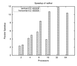
(a) radikal

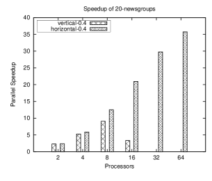
(b) 20-newsgroups

Figure 3: Parallel speedup of horizontal and vertical algorithms on small datasets radikal and 20-newsgroups

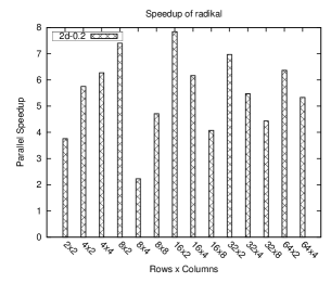
(a) radikal

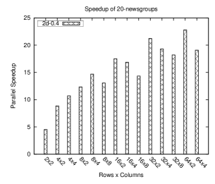
(b) 20-newsgroups

Figure 4: Parallel speedup of the 2D algorithm on small datasets radikal and 20-newsgroups

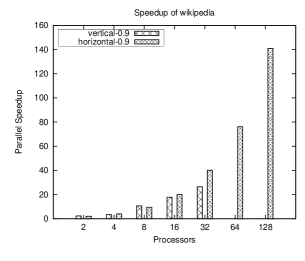
(a) wikipedia

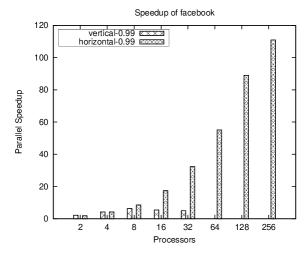
(b) facebook

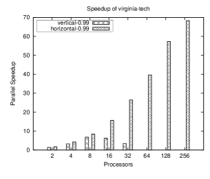
(c) virginia-tech

Figure 5: Parallel speedup of horizontal and vertical algorithms on the large datasets: wikipedia, facebook, virginia-tech

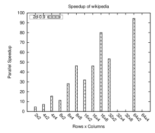
(a) wikipedia

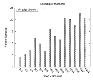
(b) facebook

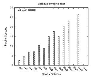
(c) virginia-tech

Figure 6: Parallel speedup of the 2D algorithm on the large datasets: wikipedia, facebook, virginia-tech

As seen in Fig. 3 and Fig. 5, we see that the horizontal algorithm scales better than the vertical algorithm for all datasets. The vertical algorithm scales well up to $8$ processors, but after that it loses quite a bit of steam. It is still quite an achievement that the vertical algorithm scales as much, since the number of processors increase the communication volume and communication asynchrony rapidly despite the local pruning optimization. The horizontal algorithm scales well up to $32$ processors and then starts to slow down due to the fact that the broadcast starts becoming significant. This is most apparent in radikal dataset, but it is also seen in other datasets that the speedup does not accelerate as much, as we go up to $64$ processors. We observe that both vertical and horizontal parallelizations achieve super-linear speedups in several cases, affirming the efficiency of our implementation, as in those cases the algorithms make better use of the memory hierarchy. In two cases, we see that the vertical algorithm achieves better speedup than the horizontal algorithm, justifying the usefulness of our vertical algorithm.

The 2-D algorithm shows varying performance according to the processor configuration as seen in Fig. 4 and Fig. 6 . Since the vertical algorithm did not scale further than $8$ processors, we did not try more processor columns in the virtual mesh. We sometimes see excellent speedups with the 2-D algorithm, for instance in wikipedia, $4\times 4$ yields super-linear speedup and $16\times 8$ yields about $80$ speedup. However, on the average, the 2-D algorithm’s performance is between that of the horizontal and vertical algorithms, it is usually better than half of the speedup of the horizontal algorithm for the maximum number of processors although for facebook dataset it’s slightly worse than that.

7.5 Local pruning and block processing optimizations

It is useful to understand the performance impact of local pruning and block processing optimizations for the vertical algorithm. Without those optimizations, the vertical algorithm is futile, it would not be quite possible to apply it to sufficiently many cases. Therefore, we show its performance, when neither optimization is applied, and when only local pruning is applied, together with happens when both optimizations are turned on.

We have chosen the smaller two datasets radikal and 20-newsgroups for this comparison, because some of the runs would be infeasible for the larger datasets. We run them on up to $16$ processors, which is sufficient to illustrate the performance differences. Fig. 7 shows how speedup varies for different vertical algorithms on small datasets, comparing the unoptimized vertical algorithm (vertical-noopt), the vertical algorithm with local pruning optimization only (vertical-localpruning) and the vertical algorithm with both local pruning and block processing optimizations applied (vertical-bothopt). It is clearly seen that local pruning improves over no optimization and both optimizations together improve on local pruning only. Local pruning is more significant for smaller number of processors and block processing is more significant for larger number of processors. In fact, without these optimizations, we see that the speedups would be too low. It is only due to these effective optimizations that we have been able to obtain the speedups previously demonstrated. The comparison is similar across two datasets. The optimizations are most effective on $8$ processors; on $16$ processors, the effectiveness of the local pruning algorithm declines greatly, which is why we did not extend the study to a larger number of processors.

Fig. 8 shows the speedups for various block sizes on small datasets. We have used block sizes of $1$, $4$, $8$, $16$, $32$, $64$ on up to $16$ processors. We have observed that increasing the block size does improve the speedup, especially on larger number of processors. Speedup generally improves on both datasets until $32$ block size, and on most until $64$ block size (except one data point); though we also observe that the gains start diminishing at $64$, which is why we stopped there. Also, larger block sizes turned out to be infeasible for large datasets.

Comparing speedups alone does not give us much insight into how these speed differences occur. We have thus profiled the algorithms in detail. We have measured the time elapsed for both communication and computation phases in the algorithms. We have also calculated how the number of candidates vary when we use the optimizations, and how many scores are actually accumulated. We have also put a barrier before each collective communication operation, so that we can measure how much processors wait before engaging in actual communication. We give both average and maximum values for the measured values, to show how imbalance for these values vary. In Table 5, Table 6, Table 7, and Table 8 we measure the following parameters for varying number of processors and algorithms: p shows the number of processors, Algo. shows the algorithm being used, $C_{avg}$ shows the average time of communication, $C_{max}$ shows the maximum time of communication, $W_{avg}$ shows the average time of work, $W_{max}$ shows the maximum time of work, Scores shows the total number of scores communicated, $Cand_{avg}$ shows the average number of candidates, $Cand_{max}$ shows the maximum number of candidates $Barr_{avg}$ shows the average barrier time, $Barr_{max}$ shows the maximum barrier time.

Table 5 and Table 6 show the profiling results for the three vertical algorithm variants previously mentioned. The profiling data suggests that the local pruning optimization is effective for reducing communication time, and the number of scores communicated. On $2$ processors, we see that it reduces more than 100-fold. Even on $16$ processors, there is a 10-fold improvement on the number of scores communicated. The work time is also reduced due to fewer scores being processed. The barrier time also reduces favorably for local pruning optimization. However, block processing further reduces barrier time, and consequently, the communication time. It turns out that block processing optimization is very effective for the all-pairs similarity problem, as otherwise the effects of small communication latencies and imbalances must be aggregating. We see that the work time slightly increases, but this is offset by the huge savings in communication time. For instance, on $8$ processors, for 20-newsgroups dataset, the maximum communication time reduces from $31.22$ seconds to $7.02$ seconds, while maximum work time increases from $24.34$ seconds to $25.89$ seconds, and the barrier time reduces from $15.87$ to $5.73$. These are quite significant savings for a parallel algorithm.

Table 7 and Table 8 show the profiling results when only the processing block size is varied in the fully optimized vertical algorithm, where algorithm “vertical-bsx” means a block size of x. Note that the numbers of scores and candidates do not change in this table. We see that, generally, enlarging block size improves reduction of communication time and barrier time. The communication imbalances also follow a decreasing trend as the block size increases, which shows that our statistical reasoning works. Especially, the communication times become much more even as the block size is increased. The barrier time also follows a similar trend, but it does not become as finely balanced. The communication and barrier times are very small already even for a block size of 64, so more intelligent document partitioning methods may not be very effective in improving communication performance. We did not increase the block size much further, since every document in the block incurs a large memory penalty. We did get out of memory errors with a block size of 64 on larger datasets. In general, the block size must be specified with the dataset size in mind so as to prevent such errors.

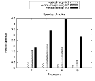
(a) radikal

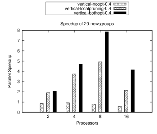
(b) 20-newsgroups

Figure 7: Speedup comparison of three parallel algorithms on radikal and 20-newsgroups datasets

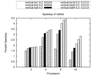
(a) radikal

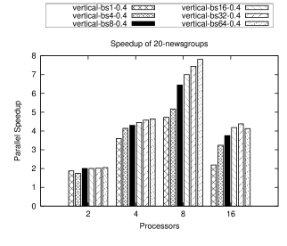
(b) 20-newsgroups

Figure 8: Speedup comparison of varying block sizes on radikal and 20-newsgroups datasets

Table 5: Profiling of vertical variants on radikal dataset

p	Algo.	$C_{avg}$	$C_{max}$	$W_{avg}$	$W_{max}$	$Barr_{avg}$	$Barr_{max}$	Scores	$Cand_{avg}$	$Cand_{max}$
2	vertical-noopt	12.03	12.09	8.63	8.71	3.15	4.42	23684403	0.0	0
2	vertical-localpruning	1.27	1.32	5.81	5.86	0.74	0.81	42086	22886.5	23272
2	vertical-bothopt	0.04	0.04	6.26	6.36	0.24	0.34	42086	22886.5	23272
4	vertical-noopt	18.41	18.72	4.12	4.28	6.69	9.98	23684403	0.0	0
4	vertical-localpruning	2.34	2.38	2.78	2.87	0.97	1.04	116000	34393.8	38986
4	vertical-bothopt	0.10	0.12	3.17	3.25	0.25	0.27	116000	34393.8	38986
8	vertical-noopt	27.15	27.91	2.02	2.16	11.47	17.21	23684403	0.0	0
8	vertical-localpruning	4.55	4.60	1.55	1.65	1.51	1.93	355937	53711.8	73642
8	vertical-bothopt	0.41	0.51	1.87	2.02	0.42	0.60	355937	53711.8	73642
16	vertical-noopt	47.35	48.04	1.21	1.55	10.57	13.52	23684403	0.0	0
16	vertical-localpruning	17.07	17.36	0.93	1.06	1.69	2.90	1155714	89717.0	202112
16	vertical-bothopt	2.42	2.57	1.23	1.35	0.54	0.89	1155714	89717.0	202112

Table 6: Profiling of vertical variants on 20-newsgroups dataset

p	Algo.	$C_{avg}$	$C_{max}$	$W_{avg}$	$W_{max}$	$Barr_{avg}$	$Barr_{max}$	Scores	$Cand_{avg}$	$Cand_{max}$
2	vertical-noopt	123.08	124.63	153.79	155.23	34.17	44.30	194138198	0.0	0
2	vertical-localpruning	12.84	14.91	134.68	136.86	10.84	12.84	287786	148376.0	246016
2	vertical-bothopt	0.17	0.18	137.88	139.72	3.29	5.13	287786	148376.0	246016
4	vertical-noopt	177.56	178.94	78.42	79.00	70.60	99.58	188179681	0.0	0
4	vertical-localpruning	18.67	19.49	54.76	56.04	14.04	14.55	1060564	274885.0	398405
4	vertical-bothopt	0.81	1.04	56.62	57.79	4.03	4.79	1060564	274885.0	398405
8	vertical-noopt	266.82	274.48	42.87	62.64	114.28	158.89	180315935	0.0	0
8	vertical-localpruning	30.78	31.22	23.33	24.34	13.79	15.87	4165217	551323.0	1939290
8	vertical-bothopt	6.19	7.02	25.22	25.89	4.83	5.73	4165217	551323.0	1939290
16	vertical-noopt	434.75	440.22	22.93	23.98	120.81	144.17	172874767	0.0	0
16	vertical-localpruning	111.18	111.83	16.82	18.08	13.58	17.53	17454734	1203360.0	11294606
16	vertical-bothopt	47.05	48.16	15.53	19.16	5.40	6.87	17454734	1203360.0	11294606

Table 7: Profiling of various block sizes on radikal dataset

p	Algo.	$C_{avg}$	$C_{max}$	$W_{avg}$	$W_{max}$	$Barr_{avg}$	$Barr_{max}$	Scores	$Cand_{avg}$	$Cand_{max}$
2	vertical-bs1	0.73	0.74	6.48	6.61	0.90	0.99	42086	22886.5	23272
2	vertical-bs4	0.23	0.23	6.36	6.47	0.52	0.61	–	–	–
2	vertical-bs8	0.12	0.13	6.35	6.38	0.34	0.36	–	–	–
2	vertical-bs16	0.08	0.08	6.33	6.45	0.34	0.45	–	–	–
2	vertical-bs32	0.05	0.05	6.32	6.34	0.29	0.31	–	–	–
2	vertical-bs64	0.04	0.04	6.29	6.33	0.23	0.25	–	–	–
4	vertical-bs1	1.78	1.87	3.40	3.48	1.34	1.43	116000	34393.8	38986
4	vertical-bs4	0.50	0.52	3.29	3.36	0.67	0.76	–	–	–
4	vertical-bs8	0.28	0.30	3.22	3.29	0.42	0.47	–	–	–
4	vertical-bs16	0.20	0.23	3.20	3.29	0.36	0.41	–	–	–
4	vertical-bs32	0.14	0.16	3.17	3.26	0.27	0.31	–	–	–
4	vertical-bs64	0.10	0.11	3.16	3.26	0.24	0.28	–	–	–
8	vertical-bs1	3.61	3.91	2.02	2.16	1.94	2.27	355937	53711.8	73642
8	vertical-bs4	1.10	1.24	1.94	2.06	1.03	1.21	–	–	–
8	vertical-bs8	0.73	0.87	1.92	2.07	0.94	1.13	–	–	–
8	vertical-bs16	0.50	0.64	1.90	2.04	0.60	0.81	–	–	–
8	vertical-bs32	0.40	0.51	1.90	2.03	0.47	0.65	–	–	–
8	vertical-bs64	0.41	0.52	1.88	2.03	0.42	0.60	–	–	–
16	vertical-bs1	15.39	16.12	1.37	1.53	2.73	3.71	1155714	89717.0	202112
16	vertical-bs4	6.39	6.66	1.31	1.45	1.17	1.69	–	–	–
16	vertical-bs8	4.77	4.95	1.29	1.42	0.97	1.40	–	–	–
16	vertical-bs16	3.57	3.74	1.28	1.43	0.85	1.25	–	–	–
16	vertical-bs32	2.85	3.01	1.28	1.44	0.64	1.00	–	–	–
16	vertical-bs64	2.43	2.58	1.23	1.34	0.55	0.89	–	–	–

Table 8: Profiling of various block sizes on 20-newsgroups dataset

p	Algo.	$C_{avg}$	$C_{max}$	$W_{avg}$	$W_{max}$	$Barr_{avg}$	$Barr_{max}$	Scores	$Cand_{avg}$	$Cand_{max}$
2	vertical-bs1	2.66	2.69	138.96	140.97	11.56	13.88	287786	148376.0	246016
2	vertical-bs4	0.88	0.88	148.88	158.13	15.14	24.28	–	–	–
2	vertical-bs8	0.50	0.52	137.95	140.12	5.35	7.53	–	–	–
2	vertical-bs16	0.30	0.31	138.80	140.88	4.54	6.64	–	–	–
2	vertical-bs32	0.39	0.40	138.46	140.61	3.96	6.10	–	–	–
2	vertical-bs64	0.17	0.18	137.19	138.65	3.09	4.54	–	–	–
4	vertical-bs1	5.87	6.25	58.95	59.57	15.29	16.31	1060564	274885.0	398405
4	vertical-bs4	2.00	2.14	58.06	58.83	9.44	10.42	–	–	–
4	vertical-bs8	1.51	1.76	57.70	59.07	7.69	8.60	–	–	–
4	vertical-bs16	0.92	1.01	57.32	57.89	6.27	7.22	–	–	–
4	vertical-bs32	0.78	0.89	57.47	58.92	4.55	5.55	–	–	–
4	vertical-bs64	0.81	1.04	57.00	58.15	4.12	4.94	–	–	–
8	vertical-bs1	17.20	18.70	27.30	27.84	16.77	18.05	4165217	551323.0	1939290
8	vertical-bs4	11.28	12.47	28.66	35.00	15.51	18.36	–	–	–
8	vertical-bs8	8.61	9.55	26.53	27.17	9.16	9.90	–	–	–
8	vertical-bs16	6.93	7.94	26.06	26.72	7.72	8.90	–	–	–
8	vertical-bs32	6.62	7.55	25.71	26.30	5.87	6.83	–	–	–
8	vertical-bs64	6.19	7.02	25.30	25.97	4.84	5.70	–	–	–
16	vertical-bs1	92.72	96.26	20.55	21.68	18.74	21.27	17454734	1203360.0	11294606
16	vertical-bs4	59.00	61.03	18.62	20.42	10.41	12.41	–	–	–
16	vertical-bs8	50.25	52.13	17.44	19.17	7.88	9.74	–	–	–
16	vertical-bs16	44.52	46.23	16.49	18.98	6.60	8.32	–	–	–
16	vertical-bs32	43.04	44.83	15.89	18.67	5.35	7.05	–	–	–
16	vertical-bs64	47.19	48.26	15.52	19.02	5.30	7.00	–	–	–

8 Conclusions & Future Work

We have designed new parallel algorithms for the efficient practical algorithms proposed by Bayardo et. al [8]. We have compared various optimizations to the practical algorithms, and we have found that a simple optimization to all-pairs-0 which we call all-pairs-0-array gave the best results. We have been able to distribute both vectors and dimensions in a way that is faithful to the original processing order and data structures of all-pairs-0-array. The vertical parallel algorithm distributes dimensions and parallelizes the inner loop, accumulating candidates. We have proposed an effective pruning step to decrease the number of candidates communicated in this step (Lemma 1). Various optimizations and implementation choices for the vertical algorithm have been considered, including a recursive similarity match search algorithm. The horizontal parallel algorithm is easier and it parallelizes the outer loop of the algorithm. We have also proposed a 2-D parallel algorithm which combines the inner-loop and outer-loop parallelizations in an elegant fashion. Our experiments show that the variety of parallelizations is useful for large-scale similarity graph construction.

In the future, we would like to incorporate more techniques to prune candidates, and other optimizations into our framework. For instance, it may be possible to exploit the Zipf-like distribution of dimension frequencies, in a better way. Data decomposition approaches, like that of [29], may be incorporated. It may also be worthwhile to investigate the applicability of our data distribution approach to approximate similarity search and knn algorithms, as well as different algorithmic approaches to proximity search. The scalability of both the vertical and the 2-D algorithms could be improved upon. For the vertical algorithm, a better recursive local pruning algorithm could be useful, or more intelligent pruning heuristics could be discovered. For the 2-D algorithm, a better implementation could make use of asynchronous communication and burst-mode transfers. In general, it is an open problem to find the best data decomposition for parallel solutions of this problem which does not suffer from the replication bottleneck of the horizontal distribution. Our present results may lead to better solutions in that area, eventually.

References

- [1] Nir Ailon and Bernard Chazelle. Approximate nearest neighbors and the fast johnson-lindenstrauss transform. In Proceedings of the thirty-eighth annual ACM symposium on Theory of computing, STOC ’06, pages 557–563, New York, NY, USA, 2006. ACM.
- [2] Alsabti, Ranka, and Singh. An Efficient Parallel Algorithm for High Dimensional Similarity Join. In IPPS: 11th International Parallel Processing Symposium. IEEE Computer Society Press, 1998.
- [3] Alexandr Andoni and Piotr Indyk. Near-optimal hashing algorithms for approximate nearest neighbor in high dimensions. Commun. ACM, 51:117–122, January 2008.
- [4] G. Aparício, I. Blanquer, and V. Hernández. A parallel implementation of the k nearest neighbours classifier in three levels: Threads, mpi processes and the grid. In Michel Daydé, José Palma, Álvaro Coutinho, Esther Pacitti, and João Lopes, editors, High Performance Computing for Computational Science - VECPAR 2006, volume 4395 of Lecture Notes in Computer Science, pages 225–235. Springer Berlin / Heidelberg, 2007.
- [5] Sunil Arya, David M. Mount, Nathan S. Netanyahu, Ruth Silverman, and Angela Y. Wu. An optimal algorithm for approximate nearest neighbor searching in fixed dimensions. In ACM-SIAM Symposium on Discrete Algorithms, pages 573–582, 1994.
- [6] Tetsuo Asano, Desh Ranjan, Thomas Roos, Emo Welzl, and Peter Widmayer. Space filling curves and their use in the design of geometric data structures. In Ricardo Baeza-Yates, Eric Goles, and Patricio Poblete, editors, LATIN ’95: Theoretical Informatics, volume 911 of Lecture Notes in Computer Science, pages 36–48. Springer Berlin / Heidelberg, 1995.
- [7] Amit Awekar and Nagiza F. Samatova. Parallel all pairs similarity search. In Proceedings of the 2010 International Conference on Information Knowledge Engineering, Las Vegas, Nevada, USA, July.
- [8] Roberto J. Bayardo, Yiming Ma, and Ramakrishnan Srikant. Scaling up all pairs similarity search. In Proceedings of the 16th international conference on World Wide Web, WWW ’07, pages 131–140, New York, NY, USA, 2007. ACM.
- [9] Ulrik Brandes, Marco Gaertler, and Dorothea Wagner. Experiments on graph clustering algorithms. In Giuseppe Di Battista and Uri Zwick, editors, Algorithms - ESA 2003, volume 2832 of Lecture Notes in Computer Science, pages 568–579. Springer Berlin / Heidelberg, 2003.
- [10] Sergey Brin. Near neighbor search in large metric spaces. In Proceedings of the 21th International Conference on Very Large Data Bases, VLDB ’95, pages 574–584, San Francisco, CA, USA, 1995. Morgan Kaufmann Publishers Inc.
- [11] M.R. Brito, E.L. Chávez, A.J. Quiroz, and J.E. Yukich. Connectivity of the mutual k-nearest-neighbor graph in clustering and outlier detection. Statistics & Probability Letters, 35(1):33 – 42, 1997.
- [12] Benjamin Bustos and Nelson Morales. On the asymptotic behavior of nearest neighbor search using pivot-based indexes. In Proceedings of the Third International Conference on SImilarity Search and APplications, SISAP ’10, pages 33–39, New York, NY, USA, 2010. ACM.
- [13] Paul B. Callahan and S. Rao Kosaraju. A decomposition of multi-dimensional point sets with applications to k-nearest-neighbors and n-body potential fields. J. ACM, 42:546–556, 1992.
- [14] Paul B. Callahan and S. Rao Kosaraju. A decomposition of multidimensional point sets with applications to k-nearest-neighbors and n-body potential fields. J. ACM, 42:67–90, January 1995.
- [15] Edgar Chávez, Gonzalo Navarro, Ricardo Baeza-Yates, and José Luis Marroquín. Searching in metric spaces. ACM Comput. Surv., 33:273–321, September 2001.
- [16] Edgar Chávez, Gonzalo Navarro, Ricardo Baeza-Yates, and José Luis Marroquín. Searching in metric spaces. ACM Comput. Surv., 33:273–321, September 2001.
- [17] Paolo Ciaccia, Marco Patella, and Pavel Zezula. M-tree: An efficient access method for similarity search in metric spaces. In Proceedings of the 23rd International Conference on Very Large Data Bases, VLDB ’97, pages 426–435, San Francisco, CA, USA, 1997. Morgan Kaufmann Publishers Inc.
- [18] Kenneth Clarkson. Nearest-Neighbor Methods for Learning and Vision: Theory and Practice, chapter Nearest-neighbor searching and metric space dimensions. MIT Press, 2006.
- [19] T.M. Cover and P.E. Hart. Nearest neighbor pattern classification. IEEE Transactions on Information Theory, 1967.
- [20] Ronald Fagin, Ravi Kumar, and D. Sivakumar. Efficient similarity search and classification via rank aggregation. In Proceedings of the 2003 ACM SIGMOD international conference on Management of data, SIGMOD ’03, pages 301–312, New York, NY, USA, 2003. ACM.
- [21] A. Faragó, T. Linder, and G. Lugosi. Fast nearest-neighbor search in dissimilarity spaces. IEEE Trans. Pattern Anal. Mach. Intell., 15:957–962, September 1993.
- [22] E. Fix and J.L. Hodges. Discriminatory analysis, nonparametric discrimination: Consistency properties. Technical Report Technical Report 4, USAF School of Aviation Medicine, 1951.
- [23] Aristides Gionis, Piotr Indyk, and Rajeev Motwani. Similarity search in high dimensions via hashing. In Proceedings of the 25th International Conference on Very Large Data Bases, VLDB ’99, pages 518–529, San Francisco, CA, USA, 1999. Morgan Kaufmann Publishers Inc.
- [24] Antonin Guttman. R-trees: A dynamic index structure for spatial searching. In International Conference On Management of Data, pages 47–57. ACM, 1984.
- [25] Jun Hirai, Sriram Raghavan, Hector Garcia-Molina, and Andreas Paepcke. Webbase: a repository of web pages. Comput. Netw., 33:277–293, June 2000.
- [26] S Ilyinsky, M Kuzmin, A Melkov, and I Segalovich. An efficient method to detect duplicates of Web documents with the use of inverted index. 2002.
- [27] Thorsten Joachims. Transductive learning via spectral graph partitioning. In In ICML, pages 290–297, 2003.
- [28] Jon M. Kleinberg. Two algorithms for nearest-neighbor search in high dimensions. In Proceedings of the twenty-ninth annual ACM symposium on Theory of computing, STOC ’97, pages 599–608, New York, NY, USA, 1997. ACM.
- [29] Sachin Kulkarni and Ratko Orlandic. High-dimensional similarity search using data-sensitive space partitioning. In Proc. 17th Int. Conf. On Database and Expert Systems Dexa, 2006.
- [30] Eyal Kushilevitz, Rafail Ostrovsky, and Yuval Rabani. Efficient search for approximate nearest neighbor in high dimensional spaces. In Proceedings of the thirtieth annual ACM symposium on Theory of computing, STOC ’98, pages 614–623, New York, NY, USA, 1998. ACM.
- [31] Swanwa Liao, Mario A. Lopez, and Scott T. Leutenegger. High dimensional similarity search with space filling curves. In In Proceedings of the 17th International Conference on Data Engineering, pages 615–622. IEEE Computer Society, 2000.
- [32] Jimmy Lin. Brute force and indexed approaches to pairwise document similarity comparisons with mapreduce. In Proceedings of the 32nd international ACM SIGIR conference on Research and development in information retrieval, SIGIR ’09, pages 155–162, New York, NY, USA, 2009. ACM.
- [33] S. P Lloyd. Least square quantization in pcm. IEEE Transactions on Information Theory, 1982. Originally published in 1957 in Bell Telephone Laboratories Paper.
- [34] J. B. MacQueen. Some methods for classification and analysis of multivariate observations. In Proceedings of 5th Berkeley Symposium on Mathematical Statistics and Probability, page 281–297. University of California Press, 1967.
- [35] Gloria Mainar-Ruiz and Juan-Carlos Perez-Cortes. Approximate nearest neighbor search using a single space-filling curve and multiple representations of the data points. In Proceedings of the 18th International Conference on Pattern Recognition - Volume 02, ICPR ’06, pages 502–505, Washington, DC, USA, 2006. IEEE Computer Society.
- [36] R. B. Marimont and M. B. Shapir. Nearest neighbour searches and the curse of dimensionality. Journal of the Institute of Mathematics and its Applications, pages 59–70, 1979.
- [37] Victor Olman, Fenglou Mao, Hongwei Wu, and Ying Xu. Parallel clustering algorithm for large data sets with applications in bioinformatics. IEEE/ACM Trans. Comput. Biol. Bioinformatics, 6:344–352, April 2009.
- [38] Erion Plaku and Lydia E. Kavraki. Distributed computation of the knn graph for large high-dimensional point sets. J. Parallel Distrib. Comput., 67:346–359, 2007.
- [39] Donovan A. Schneider and David J. DeWitt. A performance evaluation of four parallel join algorithms in a shared-nothing multiprocessor environment. SIGMOD Rec., 18:110–121, June 1989.
- [40] A.; Skubalska-Rafajlowicz, E.; Krzyzak. Fast k-nn classification rule using metric on space-filling curves. In Pattern Recognition, 1996., Proceedings of the 13th International Conference on, pages 121–125, Aug 1996.
- [41] Pravin Vaidya. An algorithm for the all-nearest-neighbors problem. Discrete & Computational Geometry, 4:101–115, 1989. 10.1007/BF02187718.
- [42] Rares Vernica, Michael J. Carey, and Chen Li. Efficient parallel set-similarity joins using mapreduce. In Proceedings of the 2010 international conference on Management of data, SIGMOD ’10, pages 495–506, New York, NY, USA, 2010. ACM.
- [43] Jun Wang, Tony Jebara, and Shih fu Chang. Graph transduction via alternating minimization. In Proc. 25th ICML, 2008.
- [44] Roger Weber, Hans-Jörg Schek, and Stephen Blott. A quantitative analysis and performance study for similarity-search methods in high-dimensional spaces. In Proceedings of the 24rd International Conference on Very Large Data Bases, VLDB ’98, pages 194–205, San Francisco, CA, USA, 1998. Morgan Kaufmann Publishers Inc.
- [45] Peter N. Yianilos. Data structures and algorithms for nearest neighbor search in general metric spaces. In Proceedings of the Fifth Annual ACM-SIAM Symposium on Discrete Algorithms (SODA), 1993.