Accurate Spectral Numerical Schemes for Kinetic Equations with Energy Diffusion

Abstract

We examine the merits of using a family of polynomials that are orthogonal with respect to a non-classical weight function to discretize the speed variable in continuum kinetic calculations. We consider a model one-dimensional partial differential equation describing energy diffusion in velocity space due to Fokker-Planck collisions. This relatively simple case allows us to compare the results of the projected dynamics with an expensive but highly accurate spectral transform approach. It also allows us to integrate in time exactly, and to focus entirely on the effectiveness of the discretization of the speed variable. We show that for a fixed number of modes or grid points, the non-classical polynomials can be many orders of magnitude more accurate than classical Hermite polynomials or finite-difference solvers for kinetic equations in plasma physics. We provide a detailed analysis of the difference in behavior and accuracy of the two families of polynomials. For the non-classical polynomials, if the initial condition is not smooth at the origin when interpreted as a three-dimensional radial function, the exact solution leaves the polynomial subspace for a time, but returns (up to roundoff accuracy) to the same point evolved to by the projected dynamics in that time. By contrast, using classical polynomials, the exact solution differs significantly from the projected dynamics solution when it returns to the subspace. We also explore the connection between eigenfunctions of the projected evolution operator and (non-normalizable) eigenfunctions of the full evolution operator, as well as the effect of truncating the computational domain.

1 Introduction

First-principles based descriptions of transport processes in plasmas require the solution of high-dimensional kinetic equations for the phase-space distribution function [1, 2]. Often, diffusion in velocity-space plays an important physical role, as discussed in [3, 4], and references therein. For example, in kinetic turbulence, there is a cascade of energy in velocity-space in addition to real space, so velocity diffusion cuts off the cascade at small velocity scales. In this sense, velocity diffusion plays a role similar to that of viscosity in conventional hydrodynamic fluid turbulence. Just as viscosity is important in hydrodynamic turbulence no matter how large the Reynolds number, velocity diffusion is important in kinetic turbulence no matter how small the collisionality. Velocity diffusion is essential to dissipate injected energy and thereby permit a statistically steady state.

Solving these kinetic equations numerically is computationally intensive [5, 6], so an important aspect of the theoretical effort is to find new optimized discretization schemes. While high order accurate discretization schemes for the spatial variables have been succesfully used for many years, finding an ideal discretization method remains particularly challenging for the discretization of velocity space in situations involving Fokker-Planck collisions [7]. Since the Fokker-Planck collision operator has terms involving first and second order derivatives with respect to the velocity variables, the discretization method must allow accurate differentiation. The scheme must also allow accurate integration since physical quantities such as the number density, the mean fluid velocity and the pressure depend on velocity moments of the distribution function.

Recently, promising new approaches based on spectral and pseudo-spectral representations have been investigated [8, 9]. It was shown in [8] that a Hermite representation for the parallel velocity has advantages over the more common finite difference schemes used in numerical simulations. In [9], different representations for the speed coordinate are explored. It is found that because the variable has values in $[0,\infty)$ instead of the entire real axis, a little-known family of polynomials (see [10, 11, 12] and references therein) gives much better performance than finite difference schemes and schemes based on classical orthogonal polynomials. High accuracy is obtained on very coarse grids for both differentiation and integration of Maxwellian-like functions, which are the functions of interest in many applications of plasma physics [9].

The purpose of this paper is to explore the suitability of the non-classical polynomials for initial-value calculations of turbulent plasma transport in the presence of collisions [4, 13]. To do so, we consider a model one-dimensional problem describing energy diffusion due to Fokker-Planck collisions [14]:

$$\frac{\partial U}{\partial t}=\frac{1}{x^{2}}\frac{\partial}{\partial x}\left[\Psi(x)x^{2}e^{-x^{2}}\frac{\partial}{\partial x}\Big{(}e^{x^{2}}U\Big{)}\right],\qquad(x>0,\;t>0),$$ (1.1)

where

$$\Psi(x)=\frac{1}{2x^{3}}\left[\operatorname{erf}(x)-\frac{2}{\sqrt{\pi}}xe^{-x^{2}}\right],\qquad\operatorname{erf}(x)=\frac{2}{\sqrt{\pi}}\int_{0}^{x}e^{-s^{2}}\,ds.$$ (1.2)

Here, $\Psi$ differs from the usual Chandrasekhar function by an additional factor of $1/x$. Our choice to focus on this particular model problem is motivated by the following characteristic features. First, the right-hand side of (1.1) corresponds exactly to the speed variable part of the energy diffusion piece in the linearized Landau-Fokker-Planck operator for same-species collisions [4, 13]. Since many state-of-the-art plasma turbulence codes (e.g. [5, 6]) use variants of the linearized Landau-Fokker-Planck operator to describe collisions, the results presented here are directly relevant to the computational effort to simulate transport processes in plasmas. Second, the relative simplicity of (1.1) makes it possible to represent the solution semi-analytically using a spectral transform method [14], which we can then use to study the properties and accuracy of various discretization schemes. Third, (1.1) has several physically satisfying properties. Any well-behaved initial distribution function relaxes to a Maxwellian distribution function $U\propto e^{-x^{2}}$ as $t\rightarrow\infty$ (the “H-theorem”). Also, for all $t$, $\partial/\partial t\left(\int Ux^{2}dx\right)=0$, i.e. the number of particles is conserved. The best time-dependent numerical schemes are designed to satisfy these basic properties exactly [13].

While we consider a single velocity dimension in (1.1), any accurate numerical scheme for this equation is immediately applicable to simulations with more velocity dimensions and more complete collision operators, such as the operator in [4] or the linearized Fokker-Planck operator, for the following reasons. For either of these collision operators in spherical velocity coordinates, the only term involving any $\partial/\partial x$ derivatives of the distribution function is the right-hand side of (1.1). For example, in the pitch-angle diffusion term, the speed $x$ appears only as a parameter, not as a derivative. Thus, (1.1) captures nearly all the complexity associated with the $x$ coordinate in higher-dimensional kinetic problems with linearized collisions, and the issue of how best to discretize the speed coordinate is quite independent of how the other velocity coordinates are discretized. As an example of how different discretizations may be applied to the different velocity coordinates, one may refer to the time-independent problems considered in [9], in which 2D velocity space is discretized using a pseudospectral $x$ discretization related to the approach considered here, combined with a Legendre modal discretization in pitch angle. In a similar manner, time-dependent problems in a 2D velocity space could be solved by combining the $x$ discretization we consider here with a Legendre modal discretization in pitch angle (or some other pitch angle discretization.) The third velocity coordinate, gyro-angle, is often averaged out of kinetic equations in plasma physics due to rapid particle gyration in a magnetic field, but this coordinate too could be included using a tensor product approach if desired.

In this article, we compute high-accuracy solutions using a true (Galerkin) spectral method to represent the projected dynamics of (1.1). We discretize velocity space only, integrating the resulting ordinary differential equations exactly in time. In future work, we plan to adapt the methods developed here to implement exponential time differencing schemes [15] and implicit-explicit Runge-Kutta methods [16] for the time-evolution of the coupled problem. However, for the model problem (1.1), any timestepping scheme will decouple into independent eigenmodes that behave as predicted by standard linear stability theory; thus, spatial discretization is our focus here.

In a separate paper [17], pseudo-spectral methods will be developed that preserve the self-adjoint structure of the discrete evolution operator, mimicking the Galerkin operator as closely as possible. Performance on coarse grids, which is of great practical importance in high-dimensional plasma turbulence codes, will be addressed in detail there, along with comparisons with other methods. In the present article, we also look at performance on coarse grids and comparisons with existing discretization schemes (Section 4.4), but the main emphasis of the paper is on questions of convergence, discrete approximation of the continuous spectrum, and the effect of domain truncation. Except in Section 4.4, we perform calculations in quadruple-precision arithmetic to better illustrate the connection between the discrete mode amplitudes in the eigenbasis of the projected evolution operator and the continuous spectral transform of the solution [14], to demonstrate that the mode amplitudes in the orthogonal polynomial basis continue to decay exponentially to arbitrarily small scales, and to more closely monitor the effect of domain truncation. The results of Figures 2–4 and 10–12 below are similar in double-precision, with relative errors only a few times larger than machine precision, which is $2^{-52}$ in double precision versus $2^{-106}$ in the calculations shown in the figures.

While errors introduced by physical approximations in a model are typically large compared to the level of accuracy we consider here, it is important when assessing the validity of the model to be confident that the results of a numerical simulation accurately represent the equations one has discretized. An additional motivation for high accuracy is that small numerical errors can impede computation of damped eigenmodes, which are sometimes important for physical understanding [18]. In applications with more dimensions, such as gyrokinetic simulations [5, 6], lower resolution would be sufficient for routine simulations. Typically tens of modes or fewer are used in the $x$ coordinate, each with tens of degrees of freedom in the pitch-angle coordinate of velocity space, and double-precision arithmetic is sufficient.

We observe a remarkable feature of the non-classical polynomials of [9, 10]: for certain initial conditions, the exact solution (computed using an expensive spectral transform approach) leaves the subspace but returns arbitrarily closely (i.e. without losing spectral accuracy) to the solution of the projected dynamics. The situation is different for classical Hermite polynomials. While the exact solution still arrives in the subspace with spectral accuracy after some time, the projected dynamics evolves to a different location in this time, with an error that decays only algebraically as a function of the dimension of the subspace.

The structure of the article is as follows. In Sections 2 and 3, we review the construction of orthogonal polynomials and present our general method for computing solutions of (1.1) by projecting the PDE onto finite dimensional subspaces. Section 4 forms the core of the paper. In §4.1, we solve Equation (1.1) for two different initial conditions, $U(x,0)=xe^{-x^{2}}$ and $U(x,0)=x^{2}e^{-x^{2}}$. In both cases we find that the non-standard polynomials are effective at representing the solution, and that they are much more accurate than classical polynomials defined by orthogonality conditions on the interval $(-\infty,\infty)$. The improved behavior is explained by comparing the mode amplitudes in the eigenbasis of the projected evolution operator to the spectral transform of the solution, computed as described in [14]. This transform method is used in §4.2-§4.4 as an independent means of validating the accuracy of the Galerkin approach. In §4.3, we compare the discrete eigenfunctions of the projected operator with the non-normalizable eigenfunctions of the PDE to see in what sense the continuous spectrum is being approximated by a discrete one. In §4.4 we study the performance of the new family polynomials for the low grid resolutions commonly used in five-dimensional kinetic simulations of magnetized plasmas, and compare their accuracy to that of classical Hermite polynomials and the finite difference scheme used by popular gyrokinetic solvers [29, 32]. We then investigate the benefits and drawbacks of truncating the domain $[0,\infty)$ to a finite interval in §5. We summarize our results and discuss future work in §6.

2 Orthogonal Polynomials

We consider two classes of orthogonal polynomials on the positive half-line. The first, discussed by Shizgal [10] and recently applied in the context of plasma physics simulations by Landreman and Ernst [9], are orthogonal with respect to the weight function

$$\rho(x)=x^{\nu}e^{-x^{2}},\qquad\quad(x>0).$$ (2.3)

We find in A that $\nu=2$ is the best choice overall in floating point arithmetic, although part of the calculation is more accurately performed with $\nu=0$. Roundoff error aside, $\nu=2$ is also most natural since the projected dynamics involves an implicit change of basis to this case. Indeed, as explained in Section 3, $\rho(x)$ then agrees with the weight function of the Sturm-Liouville problem associated with the evolution operator on the right-hand side of (1.1). Thus, except in A, computations will be performed using the $\nu=2$ polynomials. For the remainder of the paper, this class of polynomials will be referred to as “full polynomials.”

The second class of polynomials we consider are orthogonal with respect to

$$\rho(x)=x^{\nu}e^{-x^{2}},\qquad\quad(x\in\mathbb{R})$$ (2.4)

over the whole line. However, the odd polynomials will then be discarded and the even ones restricted to $\mathbb{R}_{+}$, giving a different basis for $L^{2}(\mathbb{R}_{+};\rho\,dx)$. This basis remains complete since any function on the half-line can be extended to the whole line by even reflection, which leads to an expansion in even polynomials only. With $\nu=0$ we obtain the even Hermite polynomials (scaled to be monic), whereas with $\nu=2$ we obtain the odd Hermite polynomials divided by $2^{2j+1}x$:

$$p_{j}(x)=\left\{\begin{array}[]{ll}H_{2j}(x)/2^{2j},&\nu=0\\ H_{2j+1}(x)/(2^{2j+1}x),&\nu=2\end{array}\right\},\qquad j=0,1,2,\dots$$ (2.5)

In either case, the same $n$-dimensional subspace and projected dynamics will result when the polynomials are truncated to degree $2(n-1)$, although floating-point issues make the $\nu=2$ family more desirable to work with. For the remainder of the article, polynomials in this second class will be referred to as “even polynomials” or “classical polynomials.” We note that it is preferable to discard the odd polynomials rather than the even ones since the exact solution $u(x,t)=U(x,t)e^{x^{2}}$ satisfies $\partial u/\partial x=0$ at $x=0$ for $t>0$ rather than $u(x,t)=0$; this follows from the representation (4.37) below and the results of [14] on the behavior of bounded solutions of $Lu=\lambda u$ near $x=0$, where $L$ is defined in (3.12) below. One or the other must be discarded as the odd polynomials are not orthogonal to the even ones on the half-line.

Monic orthogonal polynomials with respect to an arbitrary weight function $\rho(x)$ may be constructed via the Stieltjes procedure [19, 20]. A number of technical challenges arise, partly due to the rapid decay of $\rho(x)=x^{\nu}e^{-x^{2}}$, which leads to overflow and underflow problems in floating point arithmetic, and partly due to poor conditioning of the recurrence

$$p_{j+1}(x)=(x-a_{j})p_{j}(x)-b_{j}p_{j-1}(x)$$ (2.6)

for small values of $x$, which amplifies roundoff errors. We overcome overflow and underflow issues by carrying an extra integer to extend the exponent range of floating point numbers in the polynomial evaluation subroutine (see [17]), and avoid ill-conditioning in the recurrence (2.6) by representing the polynomials in product form

$$p_{j}(x)=\prod_{k=1}^{j}(x-x^{(j)}_{k}).$$ (2.7)

The roots $x^{(j)}_{k}$ of $p_{j}(x)$ are the eigenvalues of the symmetric tridiagonal Jacobi matrix $A_{j}$ with entries

$$(A_{j})_{ii}=a_{i-1},\quad(1\leq i\leq j),\qquad(A_{j})_{i,i+1}=(A_{j})_{i+1,i}=\sqrt{b_{i}},\quad(1\leq i<j).$$

The coefficients $a_{j}$ and $b_{j}$ as well as the squared norms $c_{j}=\|p_{j}\|^{2}$ are computed via

$$p_{0}=1,\qquad c_{0}=\langle p_{0},p_{0}\rangle,\qquad a_{0}=\langle xp_{0},p_{0}\rangle/c_{0}$$

and the following recursion for $j=1,\dots,n$:

$$p_{j}(x)=(x-a_{j-1})p_{j-1}(x)-b_{j-1}p_{j-2}(x),\quad\;\begin{aligned} c_{j}&=\langle p_{j},p_{j}\rangle,\\ a_{j}&=\langle xp_{j},p_{j}\rangle/c_{j},\end{aligned}\quad\;b_{j}=\frac{c_{j}}{c_{j-1}},$$ (2.8)

where $b_{0}p_{-1}(x)$ is taken to be zero when $j=1$. In the floating point (as opposed to symbolic) algorithm, the formula for $p_{j}(x)$ is replaced by (2.7), and the inner products $\langle f,g\rangle=\int_{0}^{\infty}f(x)\overline{g(x)}\rho(x)\,dx$ are computed using composite Gaussian quadrature on subintervals $[x_{k}^{(j)},x_{k+1}^{(j)}]$ with endpoints taken to be the zeros of $p_{j}(x)$ together with $x_{0}^{(j)}=0$ and several additional points $x_{j+1}^{(j)}$, …, $x_{j+r}^{(j)}$ chosen to integrate the tails of the integrands accurately. See [17] for further details about this approach, and [19, 20] for additional perspective.

In what follows, it is useful to define

$$\varphi_{j}(x)=c_{j}^{-1/2}p_{j}(x),$$ (2.9)

which are (non-monic) polynomials of unit length in $L^{2}(\mathbb{R}_{+};\rho\,dx)$, and

$$\tilde{\varphi}_{j}(x):=\rho(x)^{1/2}c_{j}^{-1/2}p_{j}(x),$$ (2.10)

which are unit vectors in $L^{2}(\mathbb{R}_{+};\,dx)$ that oscillate with a fairly uniform amplitude between 0 and $x^{(j)}_{j}$ and then decay rapidly to zero, as illustrated in Figure 1. To avoid excessive notation, we use the same symbols $a_{j}$, $b_{j}$, $c_{j}$, $p_{j}(x)$, $\varphi_{j}(x)$ and $\tilde{\varphi}_{j}(x)$ in the full and even cases, with the recurrence relation (2.6) replaced, in the even case, by (4.33) below.

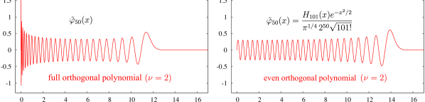
Figure 1: Re-scaled basis functions $\tilde{\varphi}_{j}(x)$ in (2.10) with $j=50$ and weight function $\rho(x)=x^{2}e^{-x^{2}}$. The main difference between the full and even polynomials is that the nodes cluster more tightly at $x=0$ in the former case, which causes the oscillations in $\tilde{\varphi}_{j}(x)$ to be less uniform. This occurs because $x=0$ is a true endpoint of the weight function in the full case and is merely a symmetry axis in the even case. Note that $\tilde{\varphi}_{j}(x)$ is odd in the even case due to the factor of $x$ in $\rho(x)^{1/2}$.

3 Projected Dynamics

The first step to solving the PDE (1.1) is to transform it to a self-adjoint system. This is done by defining

$$u(x,t)=U(x,t)e^{x^{2}},$$ (3.11)

which satisfies

$$u_{t}=-Lu,\qquad Lu=-\frac{(\Psi wu^{\prime})^{\prime}}{w},\qquad w(x)=x^{2}e^{-x^{2}},$$ (3.12)

where $u_{t}:=\partial u/\partial t$ and $u^{\prime}:=\partial u/\partial x$. Note that if $u$ and $v$ are bounded, $C^{2}$ functions on $(0,\infty)$, we have

$$\langle Lu,v\rangle=\langle u,Lv\rangle,\qquad\langle u,v\rangle=\int_{0}^{\infty}u(x)\overline{v(x)}\,w(x)\,dx.$$ (3.13)

Thus, $L$ is symmetric and densely defined on the Hilbert space

$$\mathcal{H}=L^{2}(\mathbb{R}_{+};w\,dx)=\big{\{}u\;:\;\int_{0}^{\infty}|u(x)|^{2}w(x)\,dx<\infty\big{\}}.$$ (3.14)

Physically, the $k$th moment of the distribution function $U$ may be computed as the $\mathcal{H}$-inner product of $u$ with $x^{k}$, or the $L^{2}$-inner product of $xe^{-x^{2}/2}u$ with $xe^{-x^{2}/2}x^{k}$:

$$\int_{0}^{\infty}x^{2}U(x,t)x^{k}\,dx=\langle u,x^{k}\rangle=\int_{0}^{\infty}\big{(}xe^{-x^{2}/2}u(x,t)\big{)}\big{(}xe^{-x^{2}/2}x^{k}\big{)}\,dx.$$ (3.15)

It is shown in [14] that $L$ is a singular Sturm-Liouville operator [21, 22, 23] on $(0,\infty)$ of limit circle type at $x=0$ and limit point type at $x=\infty$. The limit circle case requires a boundary condition, but it suffices to require that solutions (of $Lu=\lambda u$) remain bounded at $x=0$. The point spectrum of $L$ consists of $\lambda=0$ with eigenfunction $u\equiv 1$, and the continuous spectrum is $(0,\infty)$. A spectral transform algorithm is developed in [14] that diagonalizes the evolution operator and expresses the solution as a discrete and continuous superposition of normalizable and non-normalizable eigenfunctions of $L$. We will use this computationally expensive method to assess the accuracy of the projected dynamics below.

In this work, we approximate solutions of the PDE (3.12) by projecting onto finite dimensional subspaces of orthogonal polynomials. However, it is useful to derive the discrete evolution equations without assuming that the basis functions are polynomials (or even orthogonal). Let $\varphi_{0},\dots,\varphi_{n-1}\in\mathcal{H}$ be linearly independent and consider the subspace $\mathcal{V}=\operatorname{span}_{0\leq j<n}\varphi_{j}$. Define $\Phi:\mathbb{C}^{n}\rightarrow\mathcal{V}\subset\mathcal{H}$ and its adjoint $\Phi^{*}:\mathcal{H}\rightarrow\mathbb{C}^{n}$ by

$$(\Phi\vec{\alpha})(x)=\sum_{j=0}^{n-1}\alpha_{j}\varphi_{j}(x),\qquad(\Phi^{*}u)_{i}=\langle u,\varphi_{i}\rangle.$$ (3.16)

Let $P=\Phi(\Phi^{*}\Phi)^{-1}\Phi^{*}$ be the orthogonal projection from $\mathcal{H}$ onto $\mathcal{V}$. The projected dynamics of (3.12) onto $\mathcal{V}$ is given by

$$\partial_{t}u_{p}=-PLu_{p},$$ (3.17)

where $u_{p}$ remains in $\mathcal{V}$ for all time. In weak form, we have

$$\langle\partial_{t}u_{p},v\rangle=-\langle Lu_{p},v\rangle,\qquad(v\in\mathcal{V}).$$ (3.18)

Writing $u_{p}(x,t)=\sum_{j=0}^{n-1}\alpha_{j}(t)\varphi_{j}(x)$, we find that

$$M\vec{\alpha}_{t}=-K\vec{\alpha},$$ (3.19)

where

$$M_{ij}=\langle\varphi_{j},\varphi_{i}\rangle,\qquad K_{ij}=\langle L\varphi_{j},\varphi_{i}\rangle=\int_{0}^{\infty}\Psi(x)\varphi_{j}^{\prime}(x)\overline{\varphi_{i}^{\prime}(x)}\,w(x)\,dx$$ (3.20)

are the mass and stiffness matrices associated with the basis functions $\varphi_{j}$, respectively.

The finite-dimensional system of ODEs (3.19)–(3.20) can be solved by a wide variety of time-advance methods. We solve them exactly here in order to focus on the effectiveness of the $x$-discretization, without further complications arising from the discretization of time. Due to the linear self-adjoint structure of the equations, any other scheme will evolve the eigenmodes independently, in accordance with standard linear stability theory. Its behavior can therefore be predicted by replacing $e^{-\lambda t}$ in the spectral plots below by $R(-h\lambda)^{n}$, where $R(z)$ is the stability function of the scheme [24], $h$ is the timestep, and $n$ is the number of steps.

Since the $\varphi_{j}$ are linearly independent, $M$ is positive definite and has both a Cholesky factorization and a square root. $K$ does as well since it is positive definite on

$$\{\varphi_{0}\}^{\perp}=\{u\in\mathcal{H}\;:\;\int_{0}^{\infty}u(x)w(x)\,dx=0\},$$ (3.21)

where we assume $\varphi_{0}(x)=\text{const}.$ The Cholesky approach is more convenient for our purposes, so let us write

$$M=R_{1}^{T}R_{1},\qquad K=R_{2}^{T}R_{2},\qquad R:=R_{2}R_{1}^{-1}=USV^{T},$$ (3.22)

where the $R_{j}$ are upper-triangular and $R_{j}^{T}$ is the transpose of $R_{j}$ (or the Hermitian transpose if the basis functions are complex-valued). Assuming $\varphi_{0}$ is constant, which is convenient in practice, the first row and column of $K$ are zero. The singular value decomposition $R=USV^{T}$ solves the eigenvalue problem for $M^{-1}K$:

$$(M^{-1}K)(R_{1}^{-1}V)=(R_{1}^{-1}V)S^{2},\qquad e^{-M^{-1}Kt}=(R_{1}^{-1}V)e^{-S^{2}t}(V^{T}R_{1}).$$ (3.23)

The solution of (3.17) is then

$$u_{p}(x,t)=\Phi(x)\vec{\alpha}(t),\qquad\vec{\alpha}(t)=e^{-M^{-1}Kt}\vec{\alpha}(0),$$ (3.24)

where $\Phi(x)=(\varphi_{0}(x),\dots,\varphi_{n-1}(x))$ is treated as a row vector. Since $PL\Phi=\Phi M^{-1}K$, the eigenfunctions of $PL$ are the columns of $\Phi(x)R_{1}^{-1}V$, which are orthonormal in $\mathcal{H}$.

We note that since the constant function $\varphi_{0}$ is in the basis set, $P\varphi_{0}=\varphi_{0}$ and

$$\frac{\partial}{\partial t}\int_{0}^{\infty}x^{2}U_{p}(x,t)\,dx=\partial_{t}\langle u_{p},1\rangle=-\langle PLu_{p},1\rangle=-\langle u_{p},LP1\rangle=0,$$

i.e. mass is conserved exactly by the projected dynamics. The same is true when the domain is truncated in §5 since we impose Neumann boundary conditions at the right endpoint. The constant function remains an eigenfunction of $L$ in that case.

In floating point arithmetic, computing the SVD of $R$ is more accurate than forming $K$ and computing its eigenvalues since we avoid squaring the condition number. $R_{1}$ and $R_{2}$ can be obtained directly (without forming $M$ and $K$) as follows. First, we choose a quadrature scheme $x_{k},\mu_{k}$ such that the matrix entries $M_{ij}$, $K_{ij}$ in (3.20) are accurately approximated by

$$M_{ij}=\sum_{k=1}^{N}\varphi_{j}(x_{k})\overline{\varphi_{i}(x_{k})}w(x_{k})\mu_{k},\quad K_{ij}=\sum_{k=1}^{N}\Psi(x_{k})\varphi^{\prime}_{j}(x_{k})\overline{\varphi^{\prime}_{i}(x_{k})}w(x_{k})\mu_{k}.$$ (3.25)

We choose the $x_{k}$ and $\mu_{k}$ corresponding to the composite quadrature rule used to compute $\langle p_{j},p_{j}\rangle$ and $\langle xp_{j},p_{j}\rangle$ in (2.8) with $j=n$; see [17] for further details. Note that (3.25) may be written

$$M=E_{1}^{T}E_{1},\qquad K=E_{2}^{T}E_{2},\qquad\begin{aligned} E_{1,kj}&=\sqrt{w(x_{k})\mu_{k}}\,\varphi_{j}(x_{k}),\\ E_{2,kj}&=\sqrt{\Psi(x_{k})w(x_{k})\mu_{k}}\,\varphi^{\prime}_{j}(x_{k}).\end{aligned}$$ (3.26)

$R_{1}$ and $R_{2}$ are then obtained by QR-factorization: $E_{1}=Q_{1}R_{1}$, $E_{2}=Q_{2}R_{2}$. Since the zeroth column of $E_{2}$ is zero, we actually perform the QR factorization of columns 1 through $n-1$ to obtain $\tilde{R}_{2}$ in (3.27) below.

To reduce roundoff errors in the numerically computed singular values of $R$, we compute its pseudo-inverse before computing its SVD. In more detail, note that since $\varphi_{0}=\text{const}$,

$$R=R_{2}R_{1}^{-1}=\left(\begin{array}[]{c|c}0&0\\ \hline\cr\raisebox{-3.0pt}{$0$}&\raisebox{-3.0pt}{$\tilde{R}_{2}$}\end{array}\right)\left(\begin{array}[]{c|c}*&*\\ \hline\cr\raisebox{-3.0pt}{$0$}&\raisebox{-3.0pt}{$\tilde{R}_{1}^{-1}$}\end{array}\right)=\left(\begin{array}[]{c|c}0&0\\ \hline\cr\raisebox{-3.0pt}{$0$}&\raisebox{-3.0pt}{$\tilde{R}_{2}\tilde{R}_{1}^{-1}$}\end{array}\right)=USV^{T},$$ (3.27)

where $\tilde{R}_{j}$ is obtained from $R_{j}$ be deleting the zeroth row and column. It follows that

$$\operatorname{pinv}(R)=\left(\begin{array}[]{c|c}0&0\\ \hline\cr\raisebox{-3.0pt}{$0$}&\raisebox{-3.0pt}{$\tilde{R}_{1}\tilde{R}_{2}^{-1}$}\end{array}\right)=V\!\operatorname{pinv}(S)U^{T}.$$ (3.28)

It is well-known [25, 26, 27] that error bounds on the numerically-computed SVD of an $n\times n$ matrix $A$ are of the form $Cn^{2}\varepsilon\|A\|$, where $C$ is a constant (independent of $A$ and $n$); $\varepsilon$ is machine precision; and $\|\cdot\|$ is either the 2-norm or the Frobenius norm, depending on whether Givens rotations or Householder reflections are used in the bidiagonal reduction process. Thus, we expect that computing $V$ and $S$ via (3.28) will give better results than via (3.27) if $\|\!\operatorname{pinv}(R)\|\ll\|R\|$. We will see in A that this is the case when $\varphi_{0},\dots,\varphi_{n-1}$ are orthogonal polynomials with respect to the weight $w(x)$.

We also note that since $\tilde{R}_{1}$ and $\tilde{R}_{2}$ are upper-triangular, applying $\tilde{R}_{2}^{-1}$ to $\tilde{R}_{1}$ from the right causes information to propagate from left to right along the rows of $\tilde{R}_{1}$. More precisely, the first $j$ columns of $\tilde{R}_{1}\tilde{R}_{2}^{-1}$ do not depend on columns $k>j$ of $\tilde{R}_{1}$ or $\tilde{R}_{2}$. Thus, numerical error in high-index basis functions does not corrupt more accurately computed low-index basis functions in the initial phase of computing $\operatorname{pinv}(R)$ before performing the SVD. Sources of numerical error that tend to be larger for high-index basis functions include the process of constructing the orthogonal polynomials $\varphi_{j}(x)$, the evaluation of derivatives in the corresponding columns of $E_{2}$, and quadrature error in the formulas $M_{ij}=E_{1,:i}^{T}E_{1,:j}$ and $K_{ij}=E_{2,:i}^{T}E_{2,:j}$, where e.g. $E_{1,:j}$ denotes the $j$th column of $E_{1}$.

4 Numerical Results

We now study the accuracy of approximating solutions of $u_{t}=-Lu$ by their projected dynamics. To illustrate typical behavior, we study two initial conditions $u(x,0)=f_{j}(x)$, namely

$$\text{Example 1:}\quad f_{1}(x)=x,\qquad\quad\text{Example 2:}\quad f_{2}(x)=x^{2}.$$ (4.29)

Note that $Lf_{1}$ has a singularity at the origin, so $u_{t}(x,0)$ blows up as $x\rightarrow 0$ in that case. For this reason, Example 2 is easier and presented first below. We did not switch the labels since it is easier to remember that Example $k$ corresponds to $f(x)=x^{k}$.

The cause of the singularity in Example 1 is that $f(x)$ must be even in order to represent a smooth, radially symmetric function in three-dimensional velocity space. The reader may wonder about the physical relevance of such an initial condition. Perhaps surprisingly, this case is indeed physically relevant and occurs in several practical situations. For example, it occurs when one computes the resistivity of a plasma (see Section 3 in reference [9]) by solving the time-dependent kinetic equation for the distribution function until a steady-state is reached.

We write the solution (3.24) in the form

$$u_{p}(x,t)=\Phi(x)\vec{\alpha}(t),\qquad\vec{\alpha}(t)=Ve^{-S^{2}t}V^{T}\vec{\alpha},$$ (4.30)

where $\vec{\alpha}$ is short for $\vec{\alpha}(0)$, $V$ and $S$ were defined in (3.22), and the matrix $R_{1}$ does not appear in the second expression because $\nu=2$. Note however that, as discussed in A, the accuracy is improved if $\Phi(x)$ is corrected for loss of orthogonality by applying $R_{1}^{-1}$ from the right, where $R_{1}$ was defined in (3.22) and deviates from the identity due to orthogonality drift in floating point arithmetic. In the numerical results that follow, $\varphi_{k}$ stands for the $k$th column of $\Phi(x)R_{1}^{-1}$. See (A.44), (A.45), and the last paragraph of A for further clarification of how (4.30) is computed.

The vector $\vec{\alpha}$ can be computed analytically for the two examples in (4.29). In the full (as opposed to even) case, we have

$$x=p_{1}+a_{0},\qquad x^{2}=p_{2}+(a_{0}+a_{1})p_{1}+(a_{0}^{2}+b_{1}).$$ (4.31)

Setting $p_{j}=\sqrt{c_{j}}\varphi_{j}$ and computing $a_{j}$, $b_{j}$, $c_{j}$ via (2.8) yields

$$x =\left(\frac{1}{\pi^{1/4}}\right)\varphi_{0}+\left(\frac{\sqrt{6\pi-16}}{4\pi^{1/4}}\right)\varphi_{1},$$ (4.32)

$$x^{2} =\left(\frac{3}{4}\pi^{1/4}\right)\varphi_{0}+\left(\frac{\pi^{1/4}}{\sqrt{6\pi-16}}\right)\varphi_{1}+\left(\frac{\pi^{1/4}\sqrt{9\pi-28}}{2\sqrt{6\pi-16}}\right)\varphi_{2},$$

which give the coefficients $f(x)=\sum\alpha_{k}\varphi_{k}$.

In the even case, we note that $h_{j}(x)=H_{j}(x)2^{-j}$ are monic orthogonal polynomials with weight function $e^{-x^{2}}$ on $\mathbb{R}$ and satisfy

$$h_{0}(x)=1,\qquad h_{1}(x)=x,\qquad h_{j+1}(x)=xh_{j}(x)-\frac{j}{2}h_{j-1}(x).$$

The functions $p_{j}(x)=h_{2j+1}(x)/x$ are then orthogonal with respect to $w(x)=x^{2}e^{-x^{2}}$ on the half-line and satisfy

$$p_{0}(x)=1,\qquad p_{1}(x)=x^{2}-a_{0},\qquad p_{j+1}(x)=(x^{2}-a_{j})p_{j}(x)-b_{j}p_{j-1}(x),$$ (4.33)

where $a_{j}=\big{(}2j+\frac{3}{2}\big{)}$ and $b_{j}=j\big{(}j+\frac{1}{2}\big{)}$. It follows that $c_{j}=\|p_{j}\|^{2}$ is given by

$$c_{j}=\int_{0}^{\infty}p_{j}(x)^{2}w(x)\,dx=c_{0}\prod_{i=1}^{j}b_{i}=\frac{\sqrt{\pi}(2j+1)!}{2^{2j+2}}.$$

From $x=\sum_{j}\langle x,p_{j}\rangle c_{j}^{-1/2}\varphi_{j}$ and $x^{2}=\big{(}a_{0}\sqrt{c_{0}}\varphi_{0}+\sqrt{c_{1}}\varphi_{1}\big{)}$ we obtain

$$x=\sum_{j=0}^{\infty}\frac{(-1)^{j+1}(2j-3)!!}{\pi^{1/4}\sqrt{(2j+1)!}}\varphi_{j},\qquad x^{2}=\left(\frac{3}{4}\pi^{1/4}\right)\varphi_{0}+\left(\frac{\sqrt{6}\pi^{1/4}}{4}\right)\varphi_{1}.$$ (4.34)

An intermediate step is to show that $\langle x,p_{j}\rangle=-h_{2j}(0)/(4j-2)$. Note that $(-3)!!=-1$ and $(-1)!!=1$ in (4.34). For large $j$, Stirling’s approximation gives

$$\frac{(2j-3)!!}{\sqrt{(2j+1)!}}\approx\frac{j^{-7/4}}{(64\pi)^{1/4}}\left(1+\frac{3}{16j}+\frac{105}{512j^{2}}+\cdots\right),$$ (4.35)

so the coefficients $\alpha_{j}$ decay slowly in the even case of Example 1.

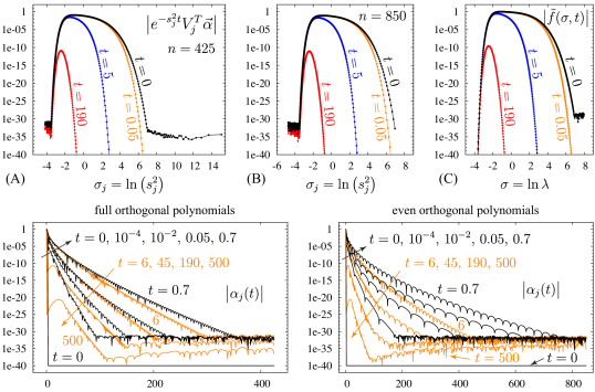
Figure 2: Evolution of mode amplitudes for Example 2 in the eigenbasis (A,B); the spectral density representation (C); and the orthogonal polynomial basis (D,E). While both sets of orthogonal polynomials are able to represent the solution of Example 2, the even polynomials require twice as many basis functions to achieve the same level of accuracy. The $s_{j}=0$ mode is excluded in (A,B).

4.1 Evolution of mode amplitudes in the eigenbasis and polynomial basis

Since the columns of $\Phi(x)V$ form an orthonormal set of eigenfunctions for $PL$ on $\mathcal{V}$, the components of the vector

$$e^{-S^{2}t}V^{T}\vec{\alpha}$$ (4.36)

represent the mode amplitudes of $u_{p}(x,t)$ in the eigenbasis while the components of $\vec{\alpha}(t)$ in (4.30) represent the mode amplitudes in the orthogonal polynomial basis. Panels (A,B,D,E) of Figure 2 show the evolution of both sets of mode amplitudes for Example 2 in the full and even cases. For comparison, we also plot the spectral transform of the solution in (C), which was computed at 512 equally spaced points between $\sigma=-4$ and $\sigma=8$ using the algorithm described in [14]. Here $\sigma=\ln\lambda$ is the spectral parameter used in [14] to represent the solution as a discrete and continuous superposition of eigenfunctions. In more detail, the solution of the PDE in the infinite dimensional space $\mathcal{H}$ may be written

$$u(x,t)=\frac{4}{\sqrt{\pi}}\hat{f}(0)+\int_{-\infty}^{\infty}v(x,\sigma)\tilde{f}(\sigma,t)\,d\sigma,$$ (4.37)

where $v(x,\sigma)=u_{1}(x,e^{\sigma})/Y(e^{\sigma})$, $u_{1}(x,\lambda)$ is a solution of $Lu=\lambda u$ with appropriate boundary conditions at $x=0$, $Y(\lambda)$ is a scale factor defined in [14],

$$\tilde{f}(\sigma,t)=\hat{f}(e^{\sigma})e^{-e^{\sigma}t}\,Y(e^{\sigma})\rho^{\prime}(e^{\sigma})e^{\sigma},\qquad\hat{f}(\lambda)=\int_{0}^{\infty}f(x)u_{1}(x,\lambda)w(x)\,dx,$$ (4.38)

and $\rho^{\prime}(\lambda)$ is the spectral density function associated with the singular Sturm-Liouville problem [21, 28, 14]. In order to understand how the results in panels A and B are related to those of panel C, consider the following. Writing $V_{j}$ for the $j$th column of $V$ and $S=\operatorname{diag}(s_{j})$, the solution of the projected dynamics is given by

$$u_{p}(x,t)=\sum_{j}v_{j}(x)\gamma_{j}(t),\qquad v_{j}(x)=\Phi(x)V_{j},\qquad\gamma_{j}=e^{-s_{j}^{2}t}V_{j}^{T}\vec{\alpha}.$$ (4.39)

Comparing (4.37) and (4.39), we can interpret the projected dynamics solution as having one component that represents $(4/\sqrt{\pi})\hat{f}(0)$ and the others approximating the integral $\int v(x,\sigma)\tilde{f}(\sigma,t)\,d\sigma$. Since the spacing of $\sigma_{j}=\ln(s_{j}^{2})$ is not uniform and the functions $v_{j}(x)$ are not normalized in the same way as $v(x,\sigma_{j})$, the vertical scaling in panels (A), (B) and (C) is not expected to be the same. Nevertheless, these graphs are remarkably similar and give insight into how the projected dynamics mimic the continuous dynamics.

Panels (D) and (E) of Figure 2 show the evolution of the coefficients $\alpha_{j}(t)$ in the orthogonal polynomial basis in the full and even cases. We added $10^{-40}$ to all the coefficients to keep the $t=0$ modes visible in the plot. In both cases, the number of active modes grows from 3 or 2 at $t=0$ to 400 or 800 at $t\approx 0.7$, then decays down to one mode (the steady state) as $t\rightarrow\infty$. The curves are plotted in black or orange depending on whether the number of active modes is growing or decaying at that time. Panels (D) and (E) show that twice as many modes are necessary to represent the solution using even polynomials instead of full polynomials. Panels (A) and (B) show why this is the case: the full polynomials are more efficient at sampling the interval $-4\leq\sigma\leq 8$ of interest. Indeed, the eigenvalue distribution in panel (B) is heavily skewed to over-sample the low end of this spectral window.

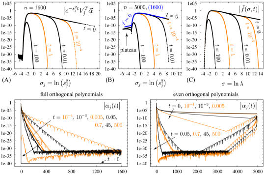
Figure 3: Evolution of mode amplitudes for Example 1 in the eigenbasis (A,B); the spectral density representation (C); and the orthogonal polynomial basis (D,E). Large errors in the mode amplitudes for small values of $s_{j}$ in panel (B) are not damped out quickly by $e^{-s_{j}^{2}t}$, and therefore persist for large times in panel (E). In panel (D), the mode amplitudes $|\alpha_{j}(t)|$ decrease until $t=0.05$ or so, then enter a brief growth period until $t=0.7$, then decay again toward steady-state.

Figure 3 shows that for Example 1 the full polynomials are again able to mimic the behavior of the continuous problem in the sense that the mode amplitudes in the eigenfunction basis closely resemble the spectral transform of the initial condition. Moreover, for $t\geq 10^{-4}$, the mode amplitudes in the orthogonal polynomial basis decay exponentially to roundoff error using 1600 modes. By contrast, in the even case, the mode amplitudes in the eigenfunction basis reach a plateau when $\sigma$ decreases below -3, and cease to resemble the spectral transform $\tilde{f}(\sigma,0)$. As a consequence, the mode amplitudes in the orthogonal polynomial basis do not decay to roundoff error accuracy until $t$ reaches $0.01$ or so, and even then the mode amplitudes $\alpha_{j}(t)$ become large again for large $j$. Thus, the even polynomials are not able to represent the solution of Example 1 effectively even for large values of $t$.

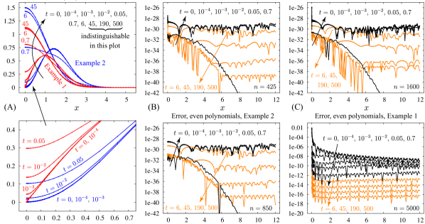
Figure 4: Evolution and error of projected dynamics in spaces of full and even orthogonal polynomials. The spectral transform approach of [14] was used for the “exact” solution. (B,C,E) both methods reach roundoff error in quadruple-precision. (F) the projected dynamics with even orthogonal polynomials does not perform well with 5000 modes until the solution approaches steady-state.

4.2 Validation of accuracy

Of course, it is not guaranteed that the full polynomials yield the correct answer for $t\geq 10^{-4}$ just because the mode amplitudes decay fast enough to reach roundoff error at that point. The true solution might leave the subspace $\mathcal{V}=\operatorname{span}\varphi_{k}$ initially and come back to a different point in the subspace than the projected dynamics predicts. This was the motivation for developing the spectral transform approach in [14], where we know the analytic form of the solution and can use it as an independent check of the correctness of the projected dynamics. In Figure 4, we plot the solution, scaled by $e^{-x^{2}/2}$, for Examples 1 and 2 at several times, together with the difference between the solution of the projected dynamics and the one obtained using the spectral transform approach, both scaled by $e^{-x^{2}/2}$. We considered other scalings, namely $e^{-x^{2}}$ (since $U=ue^{-x^{2}}$) and also $xe^{-x^{2}/2}$; the scaling $e^{-x^{2}/2}$ is the one for which the plots are the most readable. We added $(10^{-32-2x})$ to the error plots to avoid evaluating $\log_{10}(0)$ when the two methods agree to all 32 digits.

At $t=0$, both methods represent the solution with high relative accuracy for Example 2, but only the full polynomials are able to do this for Example 1. This is because the only errors at $t=0$ in panels (B,C,E) of Figure 4 are roundoff errors in the 2–3 nonzero coefficients in (4.32) and (4.34), while in panel (F) the series in (4.34) has been truncated at 5000 terms, leading to much larger errors at $t=0$. In panels (B) and (E), which correspond to Example 2, the two approaches agree to more than 28 digits of accuracy for all positive times, though twice as many modes are needed to achieve this accuracy with even polynomials. However, the errors are now absolute errors rather than relative errors. This loss of relative accuracy is expected as the spectral density approach leads to oscillatory integrals involving a large amount of cancellation to evaluate $u(x,t)e^{-x^{2}/2}$ for $t>0$ and $x\geq 6$. Similarly, the orthogonal polynomial approach yields a superposition $\sum_{j}\alpha_{j}(t)\varphi_{j}(x)e^{-x^{2}/2}$ that involves a large amount of cancellation of digits for $t>0$ and $x\geq 6$. For example, $\varphi_{j}(x)e^{-x^{2}/2}$ remains $O(1)$ well past $x=30$ when $j=425$ while $|u(x,t)e^{-x^{2}/2}|$ is less than $10^{-30}$ when $x=12$ and $t\geq 0$. For very large $t$, both methods regain high relative accuracy since the oscillatory part of the calculation becomes negligible compared to the steady-state zeroth mode. Panel (C) confirms that the full polynomials yield small (absolute) errors in Example 1 for $t\geq 10^{-4}$ even though the true solution leaves the subspace $\mathcal{V}$ for $0<t<10^{-4}$ (due to slower decay of mode amplitudes $|\alpha_{j}(t)|$ in Figure 3 than those shown for $t=10^{-4}$). Panel (F) of Figure 4 shows that this is not true for even polynomials.

There are two issues in play causing the even polynomials to be less accurate. It takes longer (by a factor of 66) for the exact solution (computed using the spectral transform method) to reach the subspace — we have checked that the distance from the exact solution to the 5000-mode even polynomial subspace does not drop below $10^{-30}$ until $t=0.0066$ — and when it arrives, the projected dynamics solution has evolved to a different location in the subspace, with an error of $1.302\times 10^{-8}$ in the $\mathcal{H}$-norm at $t=0.0066$ with 5000 modes. For comparison, the $\mathcal{H}$-norm of the exact solution at this time is $0.66354$.

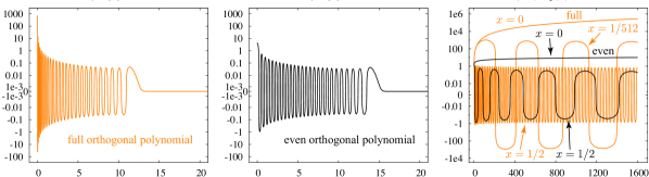
Figure 5: Full orthogonal polynomials $\varphi_{j}(x)$ (orange) grow much faster with $j$ at $x=0$ than even orthogonal polynomials (black). In panel (C), the factor of $(-1)^{j}$ is included to account for the fact that $\varphi_{j}(0)$ alternates in sign. The function $(-1)^{j}\varphi_{j}(x)e^{-x^{2}/2}$ increases monotonically in $j$ when $x=0$ is held fixed, but becomes oscillatory in $j$ for any other fixed value of $x$.

In Figure 4(B,C), the errors in the full polynomial case are much larger near $x=0$ than elsewhere. This is not a cause for concern since physical quantities, such as the moments of the distribution function in (3.15), carry an additional factor of $x^{2}$ in the integrand, which suppresses these errors. Nevertheless, it is instructive to identify their source. These errors occur because the coefficients $\alpha_{j}$ in Figures 2(D) and 3(D) carry roundoff errors that are amplified by the large values of the basis functions $\varphi_{j}(x)$ near $x=0$ for large $j$. As shown in Figure 5, $\varphi_{j}(0)$ is already close to 1000 in the full case when $j=50$, and grows to $2.8\times 10^{5}$ at $j=1600$. For other values of $x$, $(-1)^{j}\varphi_{j}(x)e^{-x^{2}/2}$ is oscillatory in $j$, with higher frequency and smaller amplitude oscillations for larger $x$. Thus, these functions are only large near $x=0$. This growth in the basis functions near $x=0$ occurs because the weight function $w(x)=x^{2}e^{-x^{2}}$ approaches 0 as $x\rightarrow 0^{+}$. Indeed, we saw in Figure 1 that when $j$ is large, $x\varphi_{j}(x)e^{-x^{2}/2}$ oscillates with a fairly uniform amplitude over a large distance before eventually decaying to zero as $x\rightarrow\infty$. In the even case, $x\varphi_{j}(x)e^{-x^{2}/2}$ resembles a sine function near $x=0$; hence, $\varphi_{j}(x)e^{-x^{2}/2}$ resembles a sinc function. However, in the full case, the zeros of $\varphi_{j}(x)$ are more tightly clustered near $x=0$ since it is a true endpoint rather than a symmetry axis. The higher oscillation rate near $x=0$ causes the peaks of $x\varphi_{j}(x)e^{-x^{2}/2}$ to be amplified more when divided by $x$ to obtain $\varphi_{j}(x)e^{-x^{2}/2}$, since $x$ is smaller at the peaks. Thus, $\varphi_{j}(0)$ grows more rapidly with $j$ in the full case than in the even case.

4.3 Eigenfunctions

Next we consider the connection between eigenfunctions of the projected operator $PL$ and solutions of $Lu=\lambda u$, which are not normalizable but serve as basis functions to represent the solution of $u_{t}=-Lu$ in a continuous superposition via the spectral transform (4.37) and (4.39). Since the exact solution has this form, one might expect that the accuracy of a discrete approximation of the continuous spectrum would be limited by the degree to which these eigenfunctions can be approximated. We find below that this is not the case: the eigenfunctions need only agree to 2–3 digits for the time dependent solutions constructed from them to agree to 30 digits.

Figure 6 shows the solution $u$ of $Lu=\lambda u$ with $u(0)=1$ and $\lambda=1$, as well as the eigenfunction $u_{p}$ of $PL$ with eigenvalue closest to 1 for two choices of $n=\dim\mathcal{V}$. One boundary condition on $u$ is sufficient at $x=0$ since the other linearly independent solution blows up there. The orange curves show the envelope of the solution of $Lu=\lambda u$, which we define as the prefactor $A_{0}p(x)$ in the asymptotic formula

$$u(x)e^{-x^{2}/2}=A_{0}p(x)\cos[q(x)+\theta_{0}]+O(x^{-15/4}).$$ (4.40)

In [14], the authors show that

$$p(x) =\textstyle x^{-1/4}\left[1+\frac{1}{8x\lambda}+\frac{5}{128x^{2}\lambda^{2}}+\frac{15}{1024x^{3}\lambda^{3}}\right],$$ (4.41)

$$q(x) =\textstyle\sqrt{2\lambda x^{5}}\left[\frac{2}{5}-\frac{1}{6x\lambda}-\frac{1}{16x^{2}\lambda^{2}}+\frac{1}{64x^{3}\lambda^{3}}+\frac{5}{3072x^{4}\lambda^{4}}+\frac{7-1152\lambda^{4}}{20480x^{5}\lambda^{5}}\right].$$ (4.42)

The parameters $A_{0}=0.443935$ and $\theta_{0}=-1.615039$ were obtained by fitting the numerical solution of $Lu=\lambda u$, $u(0)=1$, $\lambda=1$ to the form (4.40) for large $x$. Note that the amplitude of $u(x)$ decays slowly while the frequency grows rapidly since $p(x)\sim x^{-1/4}$ and $q(x)\sim x^{5/2}$.

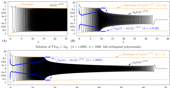
Figure 6: Comparison of eigenfunctions of $PL$ and solutions of $Lu=\lambda u$. The asymptotic formula (4.40) was used for the envelopes (orange curves) while a 15th order spectral deferred correction scheme was used to solve $Lu=\lambda u$ to plot the black curve in (A) and the blue markers in (B), (C).

The blue markers in Figure 6(B,C) show the extrema of the (highly oscillatory) residual

$$r(x)=[u_{p}(x)-u(x)]e^{-x^{2}/2}.$$

We re-scaled the eigenfunction $u_{p}$ by hand to minimize the amplitude of the oscillations in $r(x)$. Due to the logarithmic scale of the plot, it is important to use the same $\lambda$ for $u$ and $u_{p}$ when computing $r$, but setting $\lambda=1$ is sufficient for plotting the envelope. For $n=425$ (panel B of the figure), there is an interval $0.125\leq x\leq 6$ where $u_{p}$ agrees with $u$ to 2–3 digits of accuracy. For $x>6$, $r(x)$ grows in amplitude since there are not enough orthogonal polynomial basis functions for $u_{p}(x)$ to match the accelerating frequency of oscillation in $u(x)$. As a result, the blue markers move outward and begin to oscillate about the envelope curve as $u$ and $u_{p}$ pass in and out of phase with each other. At this point, the projected eigenfunction $u_{p}$ drops in amplitude by a few orders of magnitude and enters a plateau phase where it no longer reaches the envelope curve but still remains significant in size. Beyond $x=35$, the eigenfunction finally decays rapidly to zero. The results for $n=1600$ (panel C) are similar, but $|r(x)|<10^{-2}$ over a larger window $0.025<x<12.7$ and is generally 3–10 times smaller than in the $n=425$ case. The plateau region also grows from $10<x<35$ when $n=425$ to $16<x<66$ when $n=1600$.

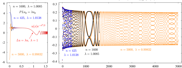
Figure 7: Gibbs overshoot phenomenon near $x=0$ (left) and coefficients $\alpha_{j}$ expressing the eigenfunctions $u_{p}$ in the orthogonal polynomial basis. The coefficients do not decay to zero as $n$ increases since $\lambda=1$ is part of the continuous spectrum of $L$, i.e. there is no normalizable eigenfunction of $L$ on $\mathbb{R}_{+}$ to which $u_{p}$ could converge.

The growth in $r(x)$ as $x\rightarrow 0^{+}$ in Figure 6(B,C) is due to a Gibbs phenomenon in the eigenfunctions of $PL$. This is shown in more detail in Figure 7(A), which plots the eigenfunction with eigenvalue closest to 1 for $n=425$ (blue), $n=1600$ (black), and $n=5000$ (orange), along with the solution $u$ of $Lu=\lambda u$, $\lambda=1$ (red). We used a linear scale on the $y$-axis to better illustrate the magnitude of the overshoot. We also plotted the results parametrically versus $x^{1/4}$ to better distinguish the oscillations from the $y$-axis and from each other. As $n$ increases, the overshoot becomes taller, narrower, and more oscillatory.

In Figure 7(B), we plot the coefficients when these eigenfunctions are expanded in the orthogonal polynomial basis. This plot illustrates that all of the eigenfunctions $u_{p}$ of $PL$ are poorly resolved in the sense that the expansion coefficients do not decay to zero once $n$ is large enough. The one exception is the $\lambda=0$ eigenfunction, $u(x)\equiv 1$, which is normalizable and agrees with $p_{0}(x)$. For the others, as $n$ increases, the higher-frequency polynomials make it possible for $u_{p}$ to match the oscillations in $u$ over a greater distance. Thus, as discussed above, the window over which $r(x)$ is small grows from $0.125<x<6$ when $n=425$, to $0.025<x<12.7$ when $n=1600$, to $0.0067<x<21$ when $n=5000$ (not shown in Figure 6). The plateau region also grows with $n$. This is a consequence of all the polynomial basis functions being present in $u_{p}$. Indeed, the effective support of $u_{p}$ (where $|u_{p}(x)e^{-x^{2}/2}|>10^{-30}$, say) is roughly the same as that of the highest frequency orthogonal polynomial present, which grows with $n$. By contrast, we will see below that on a truncated domain, the eigenfunctions of $PL$ converge to those of $L$, and are independent of $n$ once $n$ increases beyond the point where the coefficients $\alpha_{j}$ have converged to zero. It is remarkable that on the infinite domain, in spite of the Gibbs overshoot and rather poor agreement between eigenfunctions of $PL$ and solutions of $Lu=\lambda u$, the numerical solution of the projected dynamics agrees to 30 digits of accuracy to the numerically computed spectral transform solution, which is built from solutions of $Lu=\lambda u$.

4.4 Accuracy at low resolution

Numerical simulations of high dimensional kinetic equations are often so computationally intensive that only a low number of modes or grid points can be retained to discretize the speed variable. For example, in the five-dimensional gyrokinetic simulations of plasma turbulence in magnetic confinement devices, the number of grid points for the speed variable is typically 8-24 [31]. If the non-classical polynomials studied in this article are to replace existing discretization schemes for kinetic simulations, it is important to consider their performance at low resolution. In Figures 8 and 9, we compare the error at low resolution for three different discretization schemes. The first two are the full and even polynomials considered throughout the article. The third is that of the popular gyrokinetic codes GS2 and AstroGK [29, 32], in which the grid consists of $n-m$ Gauss-Legendre points on the interval $[0,2.5]$, together with $m$ Gauss-Laguerre points on $[2.5,\infty)$, where $m=1$ for $n\leq 12$ and $m=2$ otherwise [31]. In more detail, the Gauss-Laguerre points $\tilde{x}_{j}\in[0,\infty)$ are transformed to $[2.5,\infty)$ via $x_{j}=(6.25+\tilde{x}_{j}^{2})^{1/2}$, and the weights are scaled by $w_{j}=\tilde{w}_{j}/(2x_{j})$, so that $\int_{2.5}^{\infty}p(x^{2})xe^{-x^{2}}dx=\sum_{j=1}^{m}p(x_{j}^{2})x_{j}e^{-x_{j}^{2}}w_{j}$ whenever $p(\tilde{x})$ is a polynomial of degree less than $2m$. We actually used $m=\lfloor n/3\rfloor$ since the errors were smaller. In GS2 and AstroGK, the Gauss-Legendre and Gauss-Laguerre points are used for accurate numerical integration [31], but derivatives with respect to the speed variable, such as the ones appearing on the right-hand side of (1.1), are computed with a 3-point finite-difference stencil.

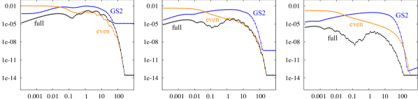
Figure 8: Evolution of the error in the Hilbert space $\mathcal{H}$ as a function of time for three discretization schemes: the full and even polynomials discussed throughout the article, and the hybrid Gauss-Legendre/Gauss-Laguerre grid used by the gyrokinetic codes GS2 and AstroGK. Here $n$ is the number of modes or grid points used to solve (1.1), the initial conditions correspond to Example 1, and the spectral transform approach of [14] was used for the “exact” solution.

Figure 8 gives the norm of the error in the Hilbert space $\mathcal{H}$ as a function of time, and Figure 9 gives the error in the computed value of $S(t)=-\int_{0}^{\infty}U^{2}x^{2}e^{x^{2}}dx$ as a function of time. $S(t)$ is an entropy-like function in the sense that it satisfies $dS/dt\geq 0$, which can be viewed as a “second principle of thermodynamics.” This can be easily seen by multiplying (1.1) by $x^{2}e^{x^{2}}U$ and integrating from $x=0$ to $x=\infty$. The initial conditions in Figures 8 and 9 are those of the more challenging Example 1, and the error is measured by comparing the solutions obtained with the three different discretization schemes with the solution obtained from the spectral transform approach. These figures show that for small grid sizes, the full polynomials are several orders of magnitude more accurate than the even polynomials for small times, and become comparable at larger times. For larger grid sizes ($n\geq 32$), the full polynomials remain more efficient than even polynomials for all time, as seen in the third panel of Figures 8 and 9, and also in Figures 2 and 3. We can also see that at a fixed grid size, the full polynomials lead to more accurate solutions than the GS2 scheme for all times, often by several orders of magnitude.

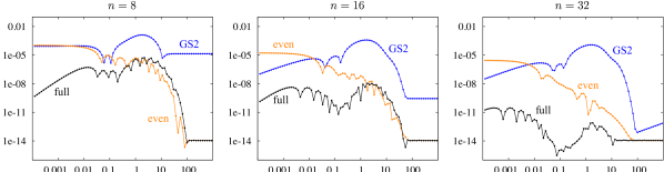
Figure 9: Evolution of the error in the entropy-like scalar function $S(t)=-\int_{0}^{\infty}U^{2}x^{2}e^{x^{2}}$ as a function of time for the discretization schemes of Figure 8. As before, $n$ is the number of modes or grid points used to solve (1.1), the initial conditions correspond to Example 1, and the spectral transform approach of [14] was used for the “exact” solution.

For the time evolution of the present paper, we evolve to any time $t$ by diagonalizing the discrete differential operators. This leads to almost no difference in the running times of GS2 and the orthogonal polynomial approach. For example, to compute the solution at all 90 values of $t$ in Figures 8 and 9, the running time (in milliseconds) of the computational phases of our two codes was

$$\begin{array}[]{c|c|c|c|c|c|c}&A\,(n=8)&B\,(n=8)&A\,(n=16)&B\,(n=16)&A\,(n=32)&B\,(n=32)\\ \hline\cr GS2&4.64&0.076&4.30&0.121&4.59&0.233\\ \hline\cr OP&3.10&0.075&2.96&0.122&3.14&0.198\end{array}$$

The columns labeled $A$ correspond either to balancing the tridiagonal matrix and computing its eigenvalues and eigenvectors (GS2 approach) or computing the SVD of $R$ in (3.27), which is precomputed and read from a file (orthogonal polynomial approach). The same file works for any $n$ (up to the one used to generate the file) since the $R$ matrices are nested. The columns labeled $B$ correspond to evolving the solution from $t=0$ to the times shown in the figures by computing $Ve^{-\Lambda t}V^{T}u_{0}$, where $V$ is the eigenvector matrix. For these small values of $n$, the running times depend more on the BLAS implementation than the number of flops involved, and the first phase (column A) is actually faster when $n=16$ than $n=8$ in both approaches. We used the Intel Math Kernel library in a C++ framework for both codes.

One advantage of the GS2 scheme is that the discretized differential operator $L$ on the right-hand side of (3.12) is tridiagonal. Thus, if the timestepping scheme of the high-dimensional problem involves solving one-dimensional subproblems (e.g. through operator splitting), the computational cost of applying $L$ or inverting $I+hL$ will be lower for GS2 than for either set of orthogonal polynomials. Thus, one could potentially use a larger $n$ in GS2 for the same computational cost as the orthogonal polynomial approach. However, increasing $n$ also increases the required storage space and communication costs, which may be more limiting resources than the CPU cycles available to solve the local one-dimensional subproblems. Nevertheless, sparse discretizations are clearly desirable. We are developing a banded version of the orthogonal polynomial approach in a pseudo-spectral framework that is more accurate than GS2 while retaining much of the sparsity advantage over the dense Galerkin approach presented here [17].

5 Truncation of the Domain

There are three benefits to truncating the domain to a finite interval. First, the method is easier to implement as the integration domain in the inner products is fixed. We continue to use a composite Gaussian quadrature rule using the zeros of $p_{n}(x)$ as the endpoints of the integration sub-intervals. However, it is no longer necessary to deal with the last sub-interval as a special case since it no longer extends to infinity. Second, the coefficients $c_{j}=\langle p_{j},p_{j}\rangle$ and $b_{j}=c_{j}/c_{j-1}$ grow less rapidly on a truncated domain. For example, numerical experiments suggest that for large $k$

$$\begin{array}[]{c|c|c}&\text{half-line}&\text{truncated to }0<x<15\\[2.0pt] \hline\cr\raisebox{-2.0pt}{$\text{even}$}&\raisebox{-2.0pt}{$b_{k}=k\big{(}k+\frac{1}{2}\big{)}$}&\raisebox{-2.0pt}{$b_{k}=14.0625+O(1/k^{2})$}\\[4.0pt] \hline\cr\raisebox{-2.0pt}{$\text{full}$}&\raisebox{-2.0pt}{$b_{k}=\frac{1}{6}(k+1)+\frac{17}{72}(k+1)^{-1}+O(1/k^{3})$}&\raisebox{-2.0pt}{$b_{k}=14.0625+O(1/k^{2})$}\end{array}.$$

Since $\|p_{j}\|^{2}=c_{j}=c_{0}\prod_{k=1}^{j}b_{j}$, we see that the monic polynomial norms grow super-exponentially on the half-line and exponentially on the truncated domain. If $n$ is not too large (say $n<400$), this alleviates the need to use special floating point numbers to guard against overflow and underflow. For larger $n$, there is little advantage in this respect. Third, orthogonal polynomials on the truncated domain are more efficient at representing functions supported near the origin since their zeros remain confined to the truncated interval, and therefore can resolve more features of the solution with fewer basis functions. On the other hand, an obvious drawback of truncating the domain is that the solution and its gradient must remain essentially zero at the right endpoint to remain a good approximation of the solution on the half-line.

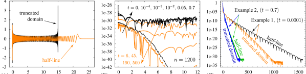
Figure 10: Plots showing the use of orthogonal polynomials on a truncated domain to solve Examples 1 and 2. The error in (B) is nearly identical to the half-line case of Figure 4(C), but only required 1200 (instead of 1600) modes. In (C), the modes decay faster on the truncated domain because the oscillations in the basis functions are more localized near the origin, as shown in (A).

In Figure 10, we illustrate these issues in the context of Examples 1 and 2, where $u(x,0)=x^{k}$, $k=1$ or $k=2$. Panel A compares the 175th normalized basis function, defined in (2.10), on the half-line and truncated domain. Both functions have 175 zeros, but they are more spread out in the half-line case. Panel B repeats the calculation of Figure 4, showing the difference between the solution obtained from the projected dynamics (this time on a truncated domain) to the spectral transform solution (plotted in Figure 4(A,D)). The errors are essentially the same as for the half-line (ranging from $10^{-26}$ near $x=0$ to $10^{-29}$ for larger $x$), but only 1200 modes were needed to reach roundoff accuracy instead of 1600. As before, with this choice of $n$, the projected dynamics solution for Example 1 is correct at $t=0$ and for $t>10^{-4}$, but not at intermediate times $0<t<10^{-4}$. Similar results, valid for $t\geq 0$, were obtained for Example 2. Panel C shows the mode amplitudes $|\alpha_{j}(t)|$ at $t=10^{-4}$ in Example 1 and $t=0.7$ for Example 2. Fewer modes are needed on the truncated domain since the zeros remain confined to $0<x<15$ in that case.

Next we look for an initial condition that is initially confined to $0<x<15$ but spreads out past the right endpoint. We tried a number of formulas and settled on a two-hump initial distribution of the form

$$u(x,0)=\begin{cases}\left[\frac{5}{2}\left(\frac{x}{3.25}\right)^{30}+\frac{155}{64}\left(\frac{x}{8.25}\right)^{200}\right]\exp\left(-\frac{15}{15-x}\right),&0<x<15,\\ 0,&\text{otherwise}.\end{cases}$$ (5.43)

The results are shown in Figure 11. Panels A and B show the solution at the times $t=0,0.05,0.7,6,45,190,500,1000,2000$, computed on the half-line, on a linear and log scale, respectively. Up until $t=6$, the solution remains confined to $0<x<15$. But then from $6<t<1000$, the solution is not negligible (in quadruple-precision) at the right endpoint. Panel C shows the difference between the truncated domain solution and the half-line solution. As expected, they agree to roundoff error for $0<t<6$, but then begin to differ near the right end of the domain due to an incorrect assumption that $u_{x}=0$ at $x=15$ in the truncated domain calculation. Once $t>1000$, the solution has decayed to the steady-state Maxwellian distribution, and the two methods agree again. Panel D shows that many fewer modes were needed to resolve the initial condition on the truncated domain than on the half-line. This is because the nodes cluster at $x=0$ and $x=15$ for the truncated domain calculation, but only at $x=0$ for the half-line calculation, and this initial condition varies rapidly near $x=15$ due to the factor of $\exp[15/(15-x)]$ in (5.43). Even in this example, where the initial distribution $u(x,t)e^{-x^{2}/2}$ has a peak of order 1 near $x=12.75$, the error in truncating the domain to $0<x<15$ was never larger than $10^{-10}$. Thus, we expect that in practice it is safe to truncate the domain as long as the initial condition and any sources are fully supported inside the truncated region.

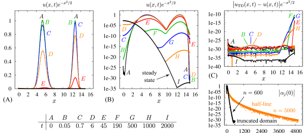
Figure 11: Evolution of two-hump initial condition that is initially contained in $0<x<15$ but eventually spreads out past the right endpoint. In panel (C), $u_{\text{TD}}(x,t)$ was computed on a truncated domain while $u(x,t)$ was computed on the half-line. The modes decay faster in (D) for the truncated domain due to clustering of the zeros of $p_{n}(x)$ near $x=15$.

As a final remark, we note that the eigenfunctions of $PL$ converge to eigenfunctions of $L$ when the domain is truncated, unlike the half-line case. This is illustrated in Figure 12. Panels A and D show the eigenmode amplitudes for Examples 1 and 2 on a half-line and truncated domain. The main difference is that on a truncated domain, further mesh refinement will not increase the density of eigenvalues of $PL$ at the left end of the spectrum since these are converged eigenvalues of the continuous problem. By contrast, on the half-line, the eigenvalues of $PL$ become more densely spaced as the mesh is refined to better approximate the continuous spectrum of $L$. In Figure 10, we saw that 1200 modes was sufficient to resolve the solution in Example 1 and 350 modes was sufficient for Example 2. In panels (B) and (E) here, we plot the eigenfunction $u_{p}$ of $PL$ with eigenvalue $\lambda$ closest to 1, re-scaled to agree as closely as possible with $u$, the solution of $Lu=\lambda u$ with the same $\lambda$ and satisfying $u(0)=1$. Note that 1200 modes yields perfect agreement between $u$ and $u_{p}$ (to 26 digits) while 350 modes yields large discrepancies: a Gibbs overshoot occurs near $x=0$, and a beat pattern appears for large $x$ where the two functions fall out of phase. The minimum amplitude of oscillation of $u_{p}-u$ in panel E is roughly $10^{-3}$ when $0.8<x<1.5$, which is 23 orders of magnitude larger than in panel B. Panels C and F show why this occurs: the solution $u$ of $Lu=\lambda u$ with $\lambda\approx 1$ requires about 500 orthogonal polynomial basis functions to be represented on $0<x<15$. When 1200 basis functions are used, the modes decay rapidly between $k=400$ and $k=500$ and the remaining modes are zero up to roundoff error. When 350 modes are used, as in Example 2, the eigenfunction of $PL$ does not agree closely with that of $L$ due to lack of resolution. However, just as in the half-line case, where none of the eigenfunctions of $PL$ agree closely with solutions of $Lu=\lambda u$, the projected dynamics is accurate to roundoff error in both examples — it is not necessary to resolve all the active eigenfunctions to accurately represent the solution of the PDE on a truncated domain either.

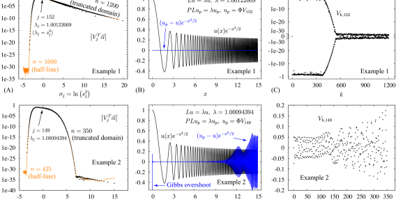
Figure 12: Comparison of mode amplitudes on a half-line and truncated domain (A,D) and plots of resolved (B) and unresolved (E) eigenfunctions of $PL$ and $L$ on $0<x<15$. As before, $V_{j}$ is the $j$th column of the matrix $V$ in the singular value decomposition $R=USV^{T}$, and $\Phi V_{j}$ is the $j$th eigenfunction of $PL$, where $\Phi=(\varphi_{0},\dots,\varphi_{n-1})$ are the orthogonal polynomials.

6 Conclusion

Shizgal [10] showed that a new class of non-classical polynomials could be used very effectively for numerical quadratures of the collision operator in kinetic simulations. More recently, Landreman and Ernst [9] showed that the same polynomials could also be much more accurate than other schemes for the discretization of the speed variable in steady-state kinetic calculations involving the collision operator. In this article, we have demonstrated that the new polynomials are also useful for time-dependent problems by examining the one-dimensional relaxation of a distribution function to a Maxwell-Boltzmann distribution via energy diffusion. We found that the new polynomials are effective at representing the solution of the partial differential equation for a wide class of initial conditions, and can be more accurate than generalized Hermite (“even”) polynomials by many orders of magnitude for the same computational work. This was seen e.g. in Fig. 2(D,E), where 350 modes are sufficient to reach errors of $10^{-30}$ with the new polynomials and $10^{-20}$ for the even polynomials, and Fig. 4(C,F), where 1600 modes with the new polynomials are $10^{20}$ times more accurate than 5000 classical modes.

Given the Sturm-Liouville structure that we associated with the problem, the polynomials defined with integration weight $\rho(x)=x^{2}e^{-x^{2}}$ are the most natural to use, and the most accurate for most parts of the computations. As discussed in A, the polynomials defined with integration weight $\rho(x)=e^{-x^{2}}$ (on the half-line), chosen for most computations in [9], also give satisfying results.

It is often the case, given the size of the numerical simulations, that one can only afford very coarse grids for a given variable. Our analysis at low resolution, in Figures 8 and 9, shows that the full polynomials are more accurate than even polynomials as well as the discretization scheme used in popular plasma kinetic codes, often by several orders of magnitude. These results, together with exact mass conservation at all times suggests that the new polynomials could be an attractive alternative to the finite difference schemes currently in use in state-of-the-art plasma microturbulence codes [5, 6]. However, for the new polynomials to make a truly compelling case, at least two questions must be answered. First, the stiffness matrix $K$ is dense, whereas finite difference matrices are sparse. Does the fact that the polynomials yield accurate results on very coarse grids compensate this disadvantage? Are there formulations based on these polynomials that can avoid operations on dense matrices? Curiously, when $\nu=0$, we find that $M$ is pentadiagonal and the entries $K_{ij}$ decay exponentially as $|i-j|$ increases, but this still leads to a much wider band of nonzero entries centered about the diagonal than in a finite-difference approach. Second, what is the best way to incorporate these polynomials in time-dependent simulations with more complete collision operators? Exponential time-differencing schemes [15] and implicit-explicit Runge-Kutta methods [16] appear promising, but this is the subject of ongoing research, with results to be reported at a later date.

7 Acknowledgments

J.W. was supported in part by the U.S. Department of Energy, Office of Science, Office of Advanced Scientific Computing Research, Applied Mathematics program under contract number DE-AC02-05CH11231, and by the National Science Foundation under Grant No. DMS-0955078. A.J.C. was supported by the U.S. Department of Energy, Office of Science, Fusion Energy Sciences under Award No. DE-FG02-86ER53223 and DE-SC0012398. M.L. was supported in part by the U.S. Department of Energy, Office of Science, Office of Fusion Energy Science, under award numbers DE-FG02-93ER54197 and DE-FC02-08ER54964.

Appendix A Effect of the choice of $\nu$ in floating-point arithmetic

In exact arithmetic, the projected dynamics onto $\mathcal{V}=\operatorname{span}\{\varphi_{0},\dots,\varphi_{n-1}\}$ is identical for any choice of $\nu$ in (2.3) since the subspace $\mathcal{V}$ consists of polynomials of degree less than or equal to $n$, regardless of the weight function. However, changing $\nu$ can have a large effect in the presence of roundoff error. To understand this, first observe that using a monomial basis for $\mathcal{V}$ (instead of orthogonal polynomials) would lead to numerical difficulties as the basis functions become nearly linearly dependent in $\mathcal{H}=L^{2}(\mathbb{R}_{+};w\,dx)$. Using orthogonal polynomials with weight exponent $\nu\neq 2$ has the potential to cause similar difficulties.

In exact arithmetic, the mass matrix $M=R_{1}^{T}R_{1}$ in (3.20) is the identity when $\nu=2$ since the $\varphi_{j}$ in (2.9) are orthonormal in $\mathcal{H}$. For any other choice of $\nu$, the Cholesky factor $R_{1}$ gives the change of basis to the $\nu=2$ case:

$$\Phi^{(\nu)}=\big{(}\varphi_{0}^{(\nu)},\dots,\varphi_{n-1}^{(\nu)}\big{)}=\Phi^{(2)}R_{1}^{(\nu)},\qquad M^{(\nu)}=\int\Phi^{(\nu)\,T}\Phi^{(\nu)}w\,dx=R_{1}^{(\nu)\,T}R_{1}^{(\nu)}.$$

Similarly, $K^{(\nu)}=R_{1}^{(\nu)\,T}K^{(2)}R_{1}^{(\nu)}$ so that $R=R_{2}^{(\nu)}(R_{1}^{(\nu)})^{-1}=R_{2}^{(2)}$ in (3.22) is independent of $\nu$ (up to roundoff errors), and is largely unaffected by orthogonality drift when $\nu=2$ as long as $R_{1}^{(\nu)}$ is actually computed rather than assumed to be the identity matrix. From (3.23), the solution of the projected dynamics is

$$u_{p}(x,t)=\big{[}\underbrace{\Phi^{(\nu)}(x)(R_{1}^{(\nu)})^{-1}}_{A}\big{]}\big{[}Ve^{-{S^{2}}t}V^{T}\big{]}\big{[}\underbrace{R_{1}^{(\nu)}\vec{\alpha}^{(\nu)}}_{B}\big{]}$$ (A.44)

where $A=\Phi^{(2)}(x)$, $B=\vec{\alpha}^{(2)}=(R_{1}^{(\nu)})^{-T}\vec{\beta}^{(\nu)}$, $\vec{\beta}^{(\nu)}=M^{(\nu)}\vec{\alpha}^{(\nu)}$, and

$$\alpha^{(\nu)}_{i}=\int u_{p}(x,0)\,\overline{\varphi^{(\nu)}_{i}(x)}\,x^{\nu}e^{-x^{2}}dx,\qquad\beta^{(\nu)}_{i}=\int u_{p}(x,0)\,\overline{\varphi^{(\nu)}_{i}(x)}\,x^{2}e^{-x^{2}}dx.$$ (A.45)

Thus, if $\nu\neq 2$, the numerical algorithm performs a change of basis to the $\nu=2$ case as an intermediate step.

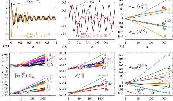
Figure 13: Comparison of roundoff errors for $\nu=0,0e,2,2^{*},2e,2e^{*},4,4e$. Here $e$ stands for “even,” $*$ stands for “assuming $R_{1}=I$,” and errors are measured against the $\nu=2$ or $\nu=2e$ quadruple-precision results. (A) and (B) show the error in using $\tilde{\Phi}^{(\nu)}(x)(R_{1}^{(\nu)})^{-1}$ with $\nu=0$ to compute $\tilde{\varphi}_{500}^{(2)}(x)$. (D) gives the sup-norm of the error in computing $\tilde{\varphi}_{k}^{(2)}(x)$ in this way. (E) shows the error in the $k$th column of $\operatorname{pinv}(R)$, as defined in (A.48). (C) and (F) give the largest and smallest singular values of $R_{1}$ and $\tilde{R}_{2}$, which help explain the results in (A), (B), (D), (E).

Figure 13 shows the sources and effect of roundoff error in evaluating the solution $u_{p}(x,t)$ via (A.44). Panels (A) and (B) show the normalized basis functions $\tilde{\varphi}_{500}^{(2)}(x)$ and $\tilde{\varphi}_{500}^{(2e)}(x)$ in (2.10) and the error in computing them in double-precision with $\nu=0$ or $\nu=0e$, where “$e$” stands for even:

$$\text{err}_{k}^{(\nu)}(x)=\operatorname{col}_{k}\big{[}\tilde{\Phi}^{(\nu)}(x)\big{(}R_{1}^{(\nu)}\big{)}^{-1}\big{]}-\tilde{\varphi}_{k}^{(2\text{ or }2e)}(x).$$ (A.46)

Here $\operatorname{col}_{k}X$ is the $k$th column of $X$. The second term on the right is the “exact” solution, which was computed with $\nu=2$ in quadruple-precision. The relative error for $k=500$ is about 60 times smaller in the even case (B) than the full case (A). This is because the orthogonal polynomials are more oscillatory near $x=0$ in the full case, where $x=0$ is a true integration boundary. A similar thing occurs in Chebyshev and Legendre polynomials, which are more oscillatory near $x=\pm 1$ than $x=0$. We plotted $\tilde{\varphi}_{500}^{(2)}(x^{2})$ in (A) to obtain more uniform oscillations for visualization.

In both (A) and (B), we note that the error has more structure than might be expected from roundoff errors alone. This is because $(R_{1}^{(\nu)})^{-1}$ is present in (A.46), which amplifies errors along singular vectors corresponding to the smallest singular values more than in other directions. (C) shows the largest and smallest singular values of $R_{1}^{(\nu)}$ as a function of $n=\dim\mathcal{V}$. Since the matrices $R_{1}^{(\nu)}$ are nested as $n$ increases, $\sigma_{\text{max}}$ is an increasing function of $n$ while $\sigma_{\text{min}}$ is decreasing. The condition number of $R_{1}^{(\nu)}$ is the ratio $\sigma_{\text{max}}/\sigma_{\text{min}}$. It is 1 for $\nu=2$, grows slowly for $\nu=0e$ and $\nu=4e$, and grows faster for $\nu=0$ and $\nu=4$. The condition number of $M$ is the square of the condition number of $R_{1}$. Thus, roundoff errors are reduced by computing $R_{1}$ directly rather than from $M$.

Panel (D) shows the max-norm of $\text{err}^{(\nu)}_{k}(x)$ as a function of $k$ for $\nu=0,2,4$ in the even and full cases. For example, the amplitudes of the largest peaks in the error curves in (A) and (B) are plotted at $k=500$ in (D) on the double-precision curves labeled $0$ and $0e$, respectively. For small values of $k$, all the values of $\nu$ that we tested yield reasonably accurate results. However, as $k$ increases, the growth in the condition number of $R_{1}^{(\nu)}$ in (C) leads to significant loss of accuracy in $\tilde{\varphi}_{k}^{(2)}$ when computed via $\tilde{\Phi}^{(\nu)}(R_{1}^{(\nu)})^{-1}$ for $\nu\neq 2$. In particular, roundoff error is amplified by more than 5 orders of magnitude with $\nu=4$ and $k=2000$. The $\nu=2$ curves (full and even) are missing from the quadruple-precision results as they are treated as “exact” solutions in (A.46). Note that even for $\nu=2$ we compute $R_{1}$ and apply its inverse to $\Phi^{(2)}$ to correct for the slight loss of orthogonality that occurs when computing the basis functions by the three-term recurrence (2.6) or (4.33). In other words, the second term in (A.46) is computed as

$$\tilde{\varphi}_{k}^{(2\text{ or }2e)}(x):=\operatorname{col}_{k}\big{[}\tilde{\Phi}^{(2\text{ or }2e)}(x)\big{(}R_{1}^{(2\text{ or }2e)}\big{)}^{-1}\big{]}.$$ (A.47)

The curves labeled $2^{*}$ and $2e^{*}$ give uncorrected results in which $R_{1}$ is assumed equal to the identity and dropped from the first term in (A.46). These errors are comparable to using $\nu=0$ or $\nu=4$, where $R_{1}$ is required.

Panel (E) shows the error in computing $\operatorname{pinv}(R)$ in (3.28). More precisely, we plot

$$E^{(\nu)}_{k}=\operatorname{col}_{k}\left[\tilde{R}^{(\nu)}_{1}(\tilde{R}^{(\nu)}_{2})^{-1}-\tilde{R}^{(2\text{ or }2e)}_{1}(\tilde{R}^{(2\text{ or }2e)}_{2})^{-1}\right],$$ (A.48)

where $\tilde{R}_{j}$ is obtained from $R_{j}$ by deleting the zeroth row and column. The second term on the right is computed in quadruple precision, and treated as “exact.” Since $R_{1}$ and $R_{2}$ are upper-triangular, the $k$th column of $E^{(\nu)}$ is independent of $n=\dim\mathcal{V}$ for $n>k$. Note that the double-precision curves labeled $\nu=0$ and $\nu=0e$ are more accurate than the $\nu=2$ and $\nu=2e$ curves, respectively. This is because we compute the SVD of $\operatorname{pinv}(R)$, which involves $R_{2}^{-1}$ rather than $R_{1}^{-1}$, and $R_{2}^{(0)}$ is better conditioned than $R_{2}^{(2)}$, as shown in panel (F). The reason is that the orthogonal polynomials for $\nu=0$ are less oscillatory near $x=0$ than for $\nu=2$ (since $\rho(x)$ vanishes at $x=0$ in the latter case), and $R_{2}$ involves derivatives of these orthogonal polynomials. Thus, a better “exact” solution would be $\nu=0$ instead of $\nu=2$ in (A.48). When this is done, the only visible effect on the plot in panel (E) is that the two most accurate quadruple-precision curves should be re-labeled (0 to 2, $0e$ to $2e$) to better account for the primary source of error in (A.48).

As mentioned previously, we compute the SVD of $\operatorname{pinv}(R)$ rather than of $R$ because $\|R\|>\|\operatorname{pinv}(R)\|$. This may be seen in panel (F), where $\sigma_{\text{max}}(\tilde{R}_{2}^{(2)})$ grows faster than $\sigma_{\text{min}}(\tilde{R}_{2}^{(2)})$ decays. (Recall that $R=R_{2}^{(2)}$ since $R_{1}^{(2)}=I$.) Also, the largest singular values of a matrix are computed with the most relative accuracy, and the largest singular values of $\operatorname{pinv}(R)$ are the ones that matter most in accurately representing solutions of the PDE (3.12).

In summary, the most accurate computation of $u_{p}(x,t)$ in (A.44) in floating point arithmetic would involve computing $A=\Phi^{(\nu)}(x)(R_{1}^{(\nu)})^{-1}$ with $\nu=2$ (without assuming $R_{1}^{(2)}=I$), and computing $V$ and $S$ from $\tilde{R}_{1}^{(\nu)}(\tilde{R}_{2}^{(\nu)})^{-1}$ with $\nu=0$. In practice we set $\nu=2$ when computing $V$ and $S$ as well since the improvement in switching to $\nu=0$ is small. The last term in (A.44), $B=\vec{\alpha}^{(2)}$, can often be computed analytically. If not, then it is most accurately computed as $B=(R_{1}^{(\nu)})^{-T}\vec{\beta}^{(\nu)}$ with $\nu=2$, including $R_{1}$ as before to account for the slight loss of orthogonality in the basis functions.

References

- [1] R. Hazeltine, J. Meiss, Plasma Confinement, Frontiers in Physics, Addison-Wesley, Redwood City, 1992.
- [2] R. Hazeltine, F. Waelbroeck, The Framework of Plasma Physics, Perseus, Reading,MA, 1998.
- [3] A. A. Schekochihin, S. C. Cowley, W. Dorland, G. W. Hammett, G. G. Howes, G. G. Plunk, E. Quataert, T. Tatsuno. Gyrokinetic turbulence: a nonlinear route to dissipation through phase space, Plasma Physics and Controlled Fusion 50 (2008) 124024.
- [4] I. Abel, M. Barnes, S. Cowley, W. Dorland, A. Schekochihin, Linearized model Fokker–Planck collision operators for gyrokinetic simulations. I. Theory, Physics of Plasmas 15 (2008) 122509.
- [5] J. Candy, C. Holland, R. Waltz, M. Fahey, E. Belli, Tokamak profile prediction using direct gyrokinetic and neoclassical simulation, Physics of Plasmas 16 (2009) 060704.
- [6] M. Barnes, I. Abel, W. Dorland, T. Görler, G. Hammett, F. Jenko, Direct multiscale coupling of a transport code to gyrokinetic turbulence codes, Physics of Plasmas 17 (2010) 056109.
- [7] P. Helander, D. Sigmar, Collisional Transport in Magnetized Plasmas, Cambridge University Press, Cambridge, 2002.
- [8] V. Bratanov, F. Jenko, D. Hatch, S. Brunner, Aspects of linear Landau damping in discretized systems, Physics of Plasmas 20 (2013) 022108.
- [9] M. Landreman, D. Ernst, New velocity-space discretization for continuum kinetic calculations and Fokker–Planck collisions, Journal of Computational Physics 243 (2013) 130–150.
- [10] B. Shizgal, A Gaussian quadrature procedure for use in the solution of the Boltzmann equation and related problems, Journal of Computational Physics 41 (1981) 309–328.
- [11] J.S. Ball, Half-range generalized Hermite polynomials and the related Gaussian quadratures, SIAM J. Numer. Anal. 40 (2003) 2311-2317
- [12] G.P. Ghiroldi, L. Gibelli, A direct method for the Boltzmann equation based on a pseudo-spectral velocity space discretization, J. Comp. Phys. 258 (2014) 568 - 584
- [13] M. Barnes, I. Abel, W. Dorland, D. Ernst, G. Hammett, P. Ricci, B. Rogers, A. Schekochihin, T. Tatsuno, Linearized model Fokker–Planck collision operators for gyrokinetic simulations. II. Numerical implementation and tests, Physics of Plasmas 16 (2009) 072107.
- [14] J. Wilkening, A. Cerfon, A Spectral Transform Method for Singular Sturm–Liouville Problems with Applications to Energy Diffusion in Plasma Physics, SIAM J. Appl. Math., (accepted), 2015.
- [15] A.-K. Kassam, L. N. Trefethen, Fourth-order time-stepping for stiff PDEs, SIAM J. Sci. Comput. 26 (4) (2005) 1214–1233.
- [16] C. A. Kennedy, M. H. Carpenter, Additive Runge-Kutta schemes for convection-diffusion-reaction equations, Appl. Numer. Math. 44 (1–2) (2003) 139–181.
- [17] J. Wilkening, A. Cerfon, M. Landreman, Symmetric pseudo-spectral velocity discretization schemes for kinetic equations with energy diffusion (in preparation).
- [18] D. R. Hatch, P. W. Terry, F. Jenko, F. Merz, W. M. Nevins, Saturation of gyrokinetic turbulence through damped eigenmodes, Phys. Rev. Lett. 106 (2011) 115003.
- [19] W. Gautschi, Construction of Gauss–Christoffel quadrature formulas, Math. Comput. 22 (1968) 251–270.
- [20] W. Gautschi, On generating orthogonal polynomials, SIAM J. Sci. Stat. Comput. 3 (3) (1982) 289–317.
- [21] E. A. Coddington, N. Levinson, Theory of Ordinary Differential Equations, Krieger Publishing Company, Malabar, Florida, 1984.
- [22] I. Stakgold, Green’s functions and boundary value problems, Wiley, New York, 1998.
- [23] M. Hajmirzaahmad, A. M. Krall, Singular second-order operators: The maximal and minimal operators, and selfadjoint operators in between, SIAM Review 34 (4) (1992) 614–634.
- [24] E. Hairer, S. P. Norsett, G. Wanner, Solving Ordinary Differential Equations I: Nonstiff Problems, 2nd Edition, Springer, Berlin, 2000.
- [25] J. Wilkening, An algorithm for computing Jordan chains and inverting analytic matrix functions, Linear Algebra Appl. 427 (2007) 6–25.
- [26] J. W. Demmel, Applied Numerical Linear Algebra, SIAM, Philadelphia, 1997.
- [27] A. J. Cox, N. J. Higham, Stability of Householder QR factorization for weighted least squares problems, in: Proceedings of the 17th Dundee Biennial Conference, Vol. 380 of Pitman Research Notes in Mathematics, Addison Wesley Longman, Harlow, Essex, UK, 1998, pp. 57–73.
- [28] C. Fulton, Titchmarsh–Weyl -functions for second-order Sturm–Liouville problems with two singular endpoints, Math. Nachr. 281 (10) (2008) 1418–1475.
- [29] M. Kotschenreuther, G. Rewoldt, W.M. Tang, Comparison of initial value and eigenvalue codes for kinetic toroidal plasma instabilities, Comput. Phys. Commun. 88 (1995) 128-140
- [30] J. Candy and R.E. Waltz, An Eulerian gyrokinetic-Maxwell solver, J. Comp. Phys. 186 (2003) 545-581
- [31] M. Barnes, W. Dorland, and T. Tatsuno, Resolving velocity space dynamics in continuum gyrokinetics, Phys. Plasmas 17 (2010), 032106
- [32] R. Numata, G.G. Howes, T. Tatsuno, M. Barnes, W. Dorland, AstroGK: Astrophysical gyrokinetics code, J. Comp. Phys. 229 (2010) 9347–9372.