Department of Mathematics Doctor of Philosophy June 2002 April 26, 2002

©   2002 William F. Bradley. All rights reserved

F. T. LeightonProfessor of Applied Mathematics

R. B. MelroseChairman, Committee on Pure Mathematics

Running in Circles:
Packet Routing on Ring Networks

I analyze packet routing on unidirectional ring networks, with an eye towards establishing bounds on the expected length of the queues. Suppose we route packets by a greedy “hot potato” protocol. If packets are inserted by a Bernoulli process and have uniform destinations around the ring, and if the nominal load is kept fixed, then I can construct an upper bound on the expected queue length per node that is independent of the size of the ring. If the packets only travel one or two steps, I can calculate the exact expected queue length for rings of any size.

I also show some stability results under more general circumstances. If the packets are inserted by any ergodic hidden Markov process with nominal loads less than one, and routed by any greedy protocol, I prove that the ring is ergodic.

For my father

Chapter 1 Statement of the Problem

1.1 The Problem

What is packet routing? In a packet routing network, we populate the nodes of a directed graph with a collection of discrete objects called packets. As time passes, these packets occasionally travel across edges, or depart the network. Sometimes, new packets are inserted. A typical question to ask is: what is the expected number of packets in the system?

This thesis is inspired by the following packet routing problem on the ring:

Suppose we have a directed graph in the form of a cycle with the edges directed clockwise. Let’s label the nodes 1 through $N$, where for $i<N$, we have a directed edge from node $i$ to $i+1$, and an additional edge from $N$ to 1. See Figure 1.1.

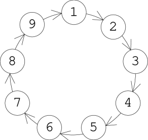
Figure 1.1: An $N=9$ node unidirectional ring

We are going to analyze the network’s behavior as it evolves in time, where time is measured in discrete steps. First, we have to specify how packets enter the ring. Let us suppose that with probability $p$, the probability that a new packet arrives at a node on one time step. With probability $1-p$, no packet arrives. This event occurs independently at every node, on every time step.

Next, we must specify how packets travel along the ring. A packet arriving at node $i$ chooses its destination uniformly from the other $N-1$ nodes. We will allow at most one packet to depart from a node in one time step. When a packet arrives at its destination, it is immediately removed; that is, a packet waiting in queue can be inserted into the ring on the same time step. Finally, if there is more than one packet at a node, we must specify which packet advances next. We’ll use the Greedy Hot Potato protocol.

Definition 1

In the Greedy Hot Potato protocol, packets travelling in the network have priority over packets waiting in queue. Nodes with non-empty queues always route packets.

This protocol for determining packet priority is called Greedy Hot Potato because a packet being passed along the ring is a “hot potato” that never stops moving until it reaches its destination. It is “greedy” in the sense that whenever a node has the opportunity to route a packet, it always takes it. This protocol resolves all contentions over which packet gets to depart from a node.

By specifying the number of packets waiting at each of the $N$ nodes, and the destination of each packet travelling in the ring, we completely specify the state of the system, and we have a discrete-time Markov chain.

Consider the number of packets in the system that need to use a node $n$. At most 1 packet can depart from $n$ on each time step. Therefore, if too many new packets arrive, the system is unstable (the Markov chain is not ergodic). In practical terms, this means that the mean total number of packets in the system will diverge to infinity with time. Let us calculate what value of $p$ corresponds to this unstable regime.

Lemma 1

Given the ring network described above, the system is unstable if $p>\frac{2}{N}$.

Proof. Consider the node $N-1$. (By symmetry of the ring, the expected number of packets that need to cross this node is the same as any other node.) If a packet arrives at node 1, it has a $1/(N-1)$ chance of needing to cross $n$. More generally, a packet arriving at node $i$ has an $i/(N-1)$ chance of needing to cross $n$, for $i<N$. Summing, the increase in congestion on $n$ by new arrivals is:

$$\sum_{i=1}^{N-1}p\frac{i}{N-1}=p\frac{N(N-1)}{2(N-1)}=p\frac{N}{2}$$

Therefore, if $p>\frac{2}{N}$, the expected number of new packets that need to cross $n$ increases by more than 1. However, the maximum possible number of packets that can cross per time step is 1. Therefore, the expected number of packets waiting to cross will increase without bound, so the system is unstable. $\Box$

If our system is stable, then, we must have $0\leq p\leq 2/N$. To make this value appear somewhat less dependent on $N$, it’s useful to define $r=p\frac{N}{2}$. We can then fix some $0\leq r\leq 1$ and study the system as $N$ gets large. This $r$ is called the nominal load.

I will call this system, as described above, the standard Bernoulli ring.

Definition 2

An $N$-node standard Bernoulli ring is an $N$-node directed cycle. Packet arrivals occur according to a Bernoulli arrival process at each node. Packet destinations are uniformly distributed. Packets are routed by the Greedy Hot Potato protocol. The nominal load $r$ is $\frac{N}{2}p$.

Coffman et al [Leighton95] made the following natural hypothesis:

Hypothesis 1

The expected queue length per node of the standard Bernoulli ring, for any fixed nominal load $0\leq r<1$, is $\Theta(1/N)$.

The authors performed extensive computer simulations that seemed to support the hypothesis. Then, in Coffman et al [Leighton98], the authors partially proved this result:

Theorem 1 (Coffman et al.)

The expected queue length per node of the standard Bernoulli ring, for any fixed nominal load $0\leq r<\frac{1}{2}$, is $\Theta(1/N)$.

Although Coffman et al. [Leighton98] established impressive results in the $r<\frac{1}{2}$ case, the $\frac{1}{2}\leq r<1$ regime was left wide open. It wasn’t even clear that the network was ergodic for any $N>2$. This thesis began as an attempt to determine the stability of the ring for values of $r$ greater than $\frac{1}{2}$, and find asymptotic bounds for the expected queue length as a function of $N$ (for a fixed $r$). As I began exploring ring networks more, I discovered that a number of interesting theorems could be proved for much more general arrival processes. This document is the result of my investigations.

1.2 What’s in this Thesis

1.2.1 A General Overview

In the earlier chapters of this thesis, I begin by examining simple ring networks. As the chapters progress, I analyze increasingly more general rings.

I begin in Chapter 2 by considering a ring network where each packet travels either 1 or 2 nodes. This type of restriction can be considered a kind of localness, where nodes only need to communicate with their nearest few neighbors. I consider a number of different routing protocols and calculate their (exact) expected queue lengths. I also calculate the stationary distribution under the GHP protocol.

In Chapter 3, I consider the standard Bernoulli ring. I prove that it is ergodic (for any $r<1$ and sufficiently large $N_{r}$), and I construct an $O(1)$ upper bound on the expected queue length per node as $N\rightarrow\infty$. This result isn’t as tight as the $O(1/N)$ upper bound postulated in Hypothesis 1, but is a first step towards achieving it. The same techniques can be applied to a host of other rings, and I discuss some of these possibilities at the end of the chapter.

In Chapter LABEL:fluid_chapter, I examine the fluid limit method introduced by Dai [Dai]. The chapter is divided into two halves. In the first half, I translate the fluid limit theorems to discrete time. This half is sufficient to prove the stability of the standard Bernoulli ring whenever $r<1$, not merely for large $N$. In the second half, I generalize the result a bit, so that (for instance) arrivals can be generated by a hidden Markov process, rather than just by arrival processes with i.i.d. interarrival times. This change leads to proofs of the stability and finiteness of expected queue length on rings much more general than the standard Bernoulli ring.

In Chapter LABEL:analytic_chapter, I translate a theorem of Zazanis [zazanis] to the discrete time case. This result shows that in the face of Bernoulli arrivals, the expected queue length of an ergodic network is an analytic function of the nominal load $r$, for $r\in[0,1)$. This means that light traffic calculations of the expected queue length are actually well defined. I can then make some explicit light traffic calculations and draw various conclusions.

The final chapter, Chapter LABEL:ringlike_chapter, concerns itself with ringlike networks, rather than rings themselves. The wrapped butterfly is an example: a $d$-dimensional wrapped butterfly shares certain features in common with a $d$-node ring, as both are regular, layered graphs with very high degrees of symmetry. I extend several of the results of the earlier sections to these more complicated topologies. I begin by proving a fluid-style stability result on all networks that use convex routing. I continue with a result about the graph structure of butterfly networks. I show that, under various conditions, a concatenated pair of butterfly graphs forms a superconcentrator. This means that we can lock down node-disjoint paths between any subset of input and output nodes (of the same size). This result is of a different flavor than the other proofs, being more graph theoretical than probabilistic.

There are also several appendices. Probability and queueing theory foundations are reviewed in Appendix LABEL:probability_chapter. For the reader unfamiliar with fluid limits, I include a complete proof of the stability results applicable for packet routing in Appendix LABEL:dummies_chapter. The results are the same as those of Dai [Dai] (actually, weaker), but the proofs are much shorter and simpler, and the Appendix is self-contained. In Appendices LABEL:fluid_limit_examples_chapter and LABEL:fluid_limit_counterexamples_chapter, I list a number of useful examples and counter-examples from the world of fluid limits. Finally, I wrote many computer programs to help me calculate stationary distributions. I discuss some of the more interesting details of this process in Appendix LABEL:computer_chapter.

For ease of reference, I have included an index. It lists the locations of definitions and main theorems.

1.2.2 The New Results

For the reader curious about which of these results are new, here is a brief list.

In Chapter 2:

• I calculate the exact expected queue length on an $N>1$ node nonstandard Bernoulli ring with parameter $L=2$, for protocols GHP, EPF, SIS, CTO, and FTG.

• I calculate the stationary distribution for the nonstandard Bernoulli ring with parameter $L=2$ for all $N$ under GHP. This result allows an exact solution for a 3 node standard Bernoulli ring, and a 5 node bidirectional standard Bernoulli ring.

In Chapter 3:

• The number of packets in one queue of a standard Bernoulli ring is bound by the number of packets in a single server queue with Bernoulli arrivals and geometric service times. An $O(1)$ bound on the expected queue length per node follows for nominal load $r<\frac{1}{2}+\epsilon$, for an explicit (but very small) $\epsilon$.

• For any $r<1$, on all sufficiently large standard Bernoulli rings, the network is ergodic. (But see the stronger results of Chapter LABEL:fluid_chapter.)

• For any $r<1$, the expected queue length per node on a standard Bernoulli ring has an $O(1)$ bound.

• For any $r<1$, the expected delay of a packet on an $N$ node standard Bernoulli ring is $\Theta(N)$.

• I briefly discuss how to extend these techniques to other Bernoulli rings:

  • For a (standard) bidirectional ring, the expected queue length per node has an $O(1)$ upper bound.

  • For an $N$ node nonstandard Bernoulli ring with parameter $L$, if $N$ is constant and $L\rightarrow\infty$, the expected queue length per node has a tight $\Theta(1)$ bound.

  • For an $N$ node nonstandard Bernoulli ring with parameter $L$, if $L$ is constant and $N\rightarrow\infty$, the expected queue length per node is lower bounded by $\Omega(1)$ and upper bounded by $O(\log(N))$.

  • Suppose that queues are finite, with some bound $B_{N}$. As $N\rightarrow\infty$, we may let $B_{N}\rightarrow\infty$. The expected queue length per node has an $O(1)$ bound.

In Chapter LABEL:fluid_chapter, determining the novelty of the results is a little bit more complicated; the proofs are very closely tied to a paper by Dai [Dai]. My own contributions amount to the following:

• I prove a discrete time fluid limit theorem. (This result is a modification of a theorem of Dai’s.)

• A corollary of the previous result is the stability of any ring, under any greedy protocol, for any maximum nominal load $r<1$.

• The fluid limit technique holds when the arrival, service, and routing processes are hidden Markov chains. This generalization of Dai’s results requires very little proof, because the hard work has already been done by Dai; only some careful definitions and reflection are needed.

In Chapter LABEL:analytic_chapter:

• I provide a rigorous justification of light traffic limits on Bernoulli rings.

• The stationary distributions for standard Bernoulli rings with $N>3$ nodes are not product form.

• The stationary distributions for geometric Bernoulli rings are not product form, except for a finite number of exceptions.

• Computer-aided calculations show that the expected queue length of a 4 node standard Bernoulli ring is not a rational function of degree less than 18.

• Consider the expected total number of packets in queue in a single-class network with rate $p$ Bernoulli arrivals. The expected value is an absolutely monotonic function of $p$.

In Chapter LABEL:ringlike_chapter:

• On any network with convex routing and nominal loads less than one, with any greedy protocol, the network is ergodic.

• Suppose we have two $d$ dimensional butterflies. Choose two permutations $\pi_{1}$ and $\pi_{2}$ on the $d$ dimensions. Then if we permute the layers of the first butterfly by $\pi_{1}$ and the second butterfly by $\pi_{2}$, and concatenate the graphs, the resulting graph is a superconcentrator.

• Suppose we take two graphs, each isomorphic to a butterfly, and concatenate them. The resulting graph concentrates subsets whose cardinality is a power of two.

The appendices are mostly abbreviated versions of material that can be found elsewhere. There are a few exceptions. Although the results in Appendix LABEL:dummies_chapter are similar to (in fact, weaker than) those of Dai [Dai], the proofs are fairly different. Several of the stability proofs from Appendix LABEL:fluid_limit_examples_chapter appear to be new, namely the theorems in Sections LABEL:LIS_stability_section and LABEL:SIS_stability_section, and the corollaries from Section LABEL:round_robin_stability_section. Finally, in Appendix LABEL:computer_chapter, Theorem LABEL:computer_theorem is new.

1.3 Ring Details

I still have to specify a few more picayune details about the ring. As mentioned before, I will be using a non-blocking model of the ring, so that if a packet departs at node $i$, then a new packet can be inserted on the same time step.

If we look at the packets waiting at a node, we will consider the packet that is about to move to be in the ring; the other packets are in queue at that node. I sometimes refer to a packet travelling in the ring as a hot potato packet.

It’s important to distinguish between the packets “at a node” and those “in queue”. The queue doesn’t include the packet (if any) in the ring, so there may be one fewer packet in queue than at the node.

In discrete time, there’s a non-zero probability that arrivals, departures and routing occur at the same time. Therefore, we have to settle on the order in which these events occur. Let us specify that one time step consists of routing current packets, possibly inducing some of them to depart, and then inserting new arrivals. On a standard Bernoulli ring, the choice of “route, then arrive” or “arrive, then route” only amounts to an $O(1/N)$ difference in the expected queue length per node, so it doesn’t really matter much which model we use.

Finally, packet routing theorists and queueing theorists tend to model packet routing problems slightly differently. Packet routing researchers like to view edges of a network as wires, and allow only one message to cross a wire at a time. Therefore, queues wait on edges. Queueing theorists, on the other hand, prefer to view packets as waiting at nodes. I will be adopting the queueing theorists’ point of view. To translate from the first perspective to the second, we can simply consider the edge graph of the packet routing network.

1.4 The Bidirectional Ring

Most of my analysis in this thesis will be directed towards the unidirectional ring, where all the packets travel in a fixed direction, e.g. clockwise. It is natural to wonder what happens if we have a bidirectional ring, where packets travel either clockwise or counterclockwise along the shortest path to their destinations. After all, this change halves the expected travel distance on the ring. In certain circumstances, we can reduce these problems to questions about the unidirectional ring.

To make this reduction, we need a slightly more general model than the standard Bernoulli ring:

Definition 3

A nonstandard Bernoulli ring with parameter L is identical to a standard Bernoulli ring, except that rather than choosing destinations uniformly from the $N-1$ nodes downstream, the destinations are chosen uniformly from the $L$ nodes downstream. (If we select $L=N-1$, we regain a standard Bernoulli ring.) The nominal load $r$ is $\frac{L+1}{2}p$.

Suppose we have an $N$-node bidirectional ring with Bernoulli arrivals. (For simplicity, imagine that $N$ is odd, so that there exists a unique shortest path between any pair of nodes.) Suppose further that there are two edges between adjacent nodes: a clockwise edge and a counterclockwise edge. That way, node $i$ can send a packet to node $i+1$ at the same time that node $i+1$ sends a packet to node $i$. Consider only the packets that travel in a clockwise direction. These packets form an $N$-node nonstandard Bernoulli ring with parameter $L=(N-1)/2$. The counterclockwise packets form the same system.

These two networks are highly dependent (after all, if a clockwise packet arrives at a node, then a counterclockwise packet cannot). However, by the linearity of expectation, the expected queue length at a node in the bidirectional ring is exactly twice the expected queue length at that node on the nonstandard Bernoulli ring with the $L$ given above. Therefore, the solutions to nonstandard Bernoulli rings in Chapters 2 and 3 translate to results about bidirectional rings.

1.5 Standardized Notation

As a kindness to the reader, I have tried to make my notation uniform throughout this thesis. In particular,

• The number of nodes in a network is $N$.

• The maximum lifespan of a packet, i.e. the longest path in the network, is $L$. (For the standard Bernoulli ring, $L=N-1$.)

• The probability of a packet arriving at a node on one time step in a Bernoulli network is $p$.

• The nominal load of a node is $r$. (For a standard Bernoulli ring, $r=\frac{N}{2}p$. For a nonstandard Bernoulli ring, $r=\frac{L+1}{2}p$.)

1.6 A Little History

There is a large literature pertaining to packet routing on ring networks. I survey some of the results that bear more directly on this thesis below.

• Coffman et al, [Leighton95] and [Leighton98], analyze the geometric Bernoulli ring:

  Definition 4

  An $N$-node geometric Bernoulli ring is an $N$-node directed cycle. Packet arrivals occur according to a Bernoulli arrival process at each node. Packet destinations are geometrically distributed. Packets are routed in a greedy fashion.

  (Unlike the standard Bernoulli ring, there is essentially only one greedy protocol on a geometric Bernoulli ring.)

  Through very careful and clever arguments, they show that a geometric Bernoulli ring has $\Theta(1/N)$ expected queue length for any nominal load $r<1$. Their argument relies on showing that the greedy protocol is optimal on geometric Bernoulli ring across a wide class of protocols, and then finding another protocol with $O(1/N)$ expected queue length. (The $\Omega(1/N)$ lower bound follows easily; see Section 3.2.)

  Coffman et al. observe that the expected queue length of a geometric Bernoulli ring with nominal load $r<1$ is an upper bound on the expected queue length of a standard Bernoulli ring with nominal load $2r$. (This fact follows readily from a stochastic dominance argument.) It follows that the expected queue length of a standard Bernoulli ring is $\Theta(1/N)$ if $0\leq r<\frac{1}{2}$.

  Why can’t we use the same techniques on the standard Bernoulli ring as we do on the geometric Bernoulli ring? Well, all the packets on a geometric Bernoulli ring are essentially indistinguishable; because of the geometric distribution on travel distances, the past history of a packet doesn’t effect its future probability of leaving the ring. This property makes stochastic dominance arguments straightforward, so it’s easy to find other, more analytically tractable protocols that can bound the expected queue length of the greedy protocol. On the other hand, the conditional probability that a packet departs the standard Bernoulli ring is very much dependent on how far it’s travelled. It is correspondingly very, very difficult to find networks that could stochastically dominate all these conditional probabilities.

  Both papers mention Hypothesis 1 as a vexing open question.

• The Greedy Hot Potato protocol may be the most natural to use on the ring, but it’s certainly not the easiest to analyze. Kahale and Leighton [kahale95] use generating functions to calculate a bound on the expected packets per node under the Farthest First protocol (where the packet with the most distant destination gets precedence over other packets.) The bound is:

  $$\frac{4r}{N}\left(\frac{1}{2(1-r)^{2}}-\frac{1}{2}\right)=O(1/N)$$

  These arguments depend very heavily on the protocol, and don’t translate to GHP.

• There are some fairly impressive and general results on stability and expected queue length on Markovian networks.

  Definition 5

  A network is Markovian if the behavior of any two packets at a queue is stochastically identical. Thus, to specify a Markov chain, it is sufficient to specify how many packets are at each node (as opposed to specifying the class of each packet). A network with this property is also called classless, or single classed.

  The geometric Bernoulli ring is an example of a Markovian network.

  The first breakthrough in the subject came from Stamoulis and Tsitsiklis [kn:j7]. They showed how to bound the expected queue length under a First In, First Out (FIFO) protocol and (continuous time) deterministic service by a processor sharing protocol with exponential service times. It’s easy to calculate the expected queue length of the latter network, so the method provides explicit upper bounds on expected total queue length in the network.

  Stamoulis and Tsitsiklis used their results on hypercubes and butterfly graphs, but their proofs clearly apply to any layered network. Mitzenmacher [kn:j6] used these results to analyze the $N\times N$ array, for instance. However, the technique broke down on networks with loops, such as rings or tori.

  This problem was very nicely resolved by Harchol-Balter [mor] in her dissertation. She showed how to construct the same simple upper bounds for any Markovian network, including those with loops.

  If we applied these results naively to a standard Bernoulli ring, we would get an $O(1)$ bound on the expected queue length per node. This result is akin to the $O(1)$ bound in Theorem 2 from Coffman et al. [Leighton95] on the geometric Bernoulli ring. Unfortunately, a standard Bernoulli ring is emphatically not Markovian, and the analysis fails.

• Since the standard Bernoulli ring model runs in discrete time, and each packet needs only one unit of time to cross an edge, it is tempting to imagine that there should be some very general solutions for the stationary probabilities, analogous to the solutions to a Kelly network in continuous time. One successful result along those lines is due to Modiano and Ephremides [modiano]. They show exact solutions for expected queue length on a tree network where all paths lead back to the root node.

  Can this result be extended for arbitrary layered graphs? Modiano believes that this is true, but the proof is non-obvious, to say the least. (If true, this would resolve an open question in Stamoulis and Tsitsiklis [kn:j7] concerning the expected queue length per node on a butterfly.) Extending it to networks with feedback, like a ring, seems impossible.

• Rene Cruz [Cruz1], [Cruz2] developed a model of packet routing with “burstiness” constraints. These constraints boil down to the following: for each edge, fix $r,s>0$. Then in $T$ time steps, at most $\lfloor Tr+s\rfloor$ packets can arrive. In Cruz [Cruz2], he proves a stability result on a model of a 4 node ring.

  Georgiadis and Tassiulas [georgiadis1] show that Cruz’s model of the ring is stable under a greedy protocol, on a ring of any size, so long as the nominal loads are less than one.

  For stochastic arrival processes like the Bernoulli process, Cruz’s burstiness assumptions are too restrictive, so his stability theorems don’t apply.

• Cruz can be considered one of the forefathers of adversarial queueing theory. The intent of adversarial queueing theory is to prove that even in the face of maliciously planned packet insertions, certain networks and protocols are still stable.

  More specifically, fix an integer $T$ and some $0\leq r\leq 1$. Imagine that an adversary injects packets such that for any fixed edge $e$, the number of packets injected during the previous $T$ time steps that need to use $e$ is less than $\lfloor rT\rfloor$. A network and protocol is stable with load $r$ if for any $T$, there is a maximum number of packets $M_{T}$ that can appear in the network simultaneously. (Thus, the adversary “wins” if he can make the number of packets in the system grow unboundedly.)

  Adversarial queueing theory was originally introduced by Borodin et al. [kn:j8]. The result of interest to us is from Andrews et al. [Andrews], where the authors show that the ring is adversarially stable under any greedy protocol, for any $r<1$. A very interesting converse was proved by Goel [Goel], who showed that any network containing more than one ring is adversarially unstable for some protocol and some $r_{0}<1$. An equivalent result for stochastic stability is unknown but desirable.

  Almost any stochastic arrival process (like the Bernoulli) has a potential for unbounded “burstiness”. This fact prevents the adversarial results from applying to a standard Bernoulli ring in any obvious way.

• Around 1995, a major advance was made in the general study of stability on queueing networks. Dai [Dai] introduced fluid limit models, a method of rescaling a stochastic system to reduce it to a deterministic one. One of the consequences of this theory was a proof that in continuous time, the (generalized Kelly) ring is stable under any greedy protocol, so long as the maximum nominal load on any node is less than one (see Dai and Weiss [Dai_and_Weiss]). Further refinements of the theory allowed proofs of the finiteness of the expected queue length assuming bounded variance of the arrival and service times of the network (see Dai and Meyn [Dai_and_Meyn]). I’ll be looking at fluid limits in greater detail in Chapter LABEL:fluid_chapter.

• Gamarnik [Gamarnik] managed to prove an adversarial fluid limit theorem, providing a way to prove adversarial stability by analyzing a more complicated fluid limit. As an example, he provided yet another proof of the adversarial stability of the ring.

Chapter 2 Exact Solutions

2.1 Introduction

In this chapter, I’m going to perform exact calculations of the expected queue length and stationary distribution of several families of rings. For a brief review of stationary distributions and discrete time Markov chains, please see Section LABEL:basic_probability_section.

Recall the nonstandard Bernoulli ring with parameter $L$ introduced in Section 1.4. A nonstandard Bernoulli ring can be specified by it’s size $N$ and its maximum path length $L$. If $L$ is fairly small relative to $N$, then we can imagine that packets only need to communicate in a small local neighborhood of themselves. If, on the other hand, $L\geq N$, then a packet can cross the same node more than once.

I can only hope to calculate exact solutions in the simplest cases; even then, some of the proofs are fairly involved. I will exactly calculate the expected queue length for the case of $N=1$ for arbitrary $L$, and $L=1$ or $2$ for arbitrary $N$. The results hold for several different protocols. I will also find the stationary distribution for $L=2$ and all $N$ under the GHP protocol.

2.2 The One Node Ring

Remember that the standard routing protocol for a ring is Greedy Hot Potato (GHP), where packets travelling in the ring have precedence over packets in queue. In a one node ring, this means that the packet which is being serviced remains in service until it leaves the queue (i.e. no pre-emptions occur.) Observe that this protocol is the same as First In, First Out (FIFO):

Definition 6

The First In, First Out (FIFO) protocol, as its name suggests, gives priority to earlier arrivals at a node. That is, the $n$th packet arriving at the node will be the $n$th packet departing. (Simultaneous arrivals are numbered randomly.) This protocol is also called First Come, First Served (FCFS).

For an $N$ node ring with $N>1$, FIFO and GHP are not the same. Note that since a packet doesn’t really “travel” anywhere on a $N=1$ node ring, some people find it might be more natural to view a packet as having an amount of work associated with it. (So, for example, rather than “travelling” in place for $k$ time steps, we say the packet has $k$ units of work.) However, I will stick with the “travel” metaphor.

Theorem 2

Suppose we have a 1 node nonstandard Bernoulli ring with parameter $L$, and we are routing using GHP. Suppose that the arrival rate is $p=\frac{2}{L+1}r$. Then the expected queue length is:

$$E[\mbox{queue length}]=\frac{L-1}{L+1}\frac{2r^{2}}{3(1-r)}$$

Note: Therefore, for a fixed $r$, the expected queue length is $O(1)$ in $L$.

Proof. Since $N=1$, we have a single server queue, and can apply standard tools from queueing theory. The ergodicity of a single server queue for nominal loads less than one follows from typical arguments (e.g. Gallager [kn:b3], Chapter 7). For the expected queue length, recall the discrete time version of the Pollaczek-Khinchin formula (Theorem LABEL:p-k_theorem):

$$E[\mbox{queue length}]=\frac{\lambda^{2}(E[Z^{2}]-E[Z])}{2(1-\lambda E[Z])}$$

where $\lambda$ is the arrival rate (i.e. $p$), and $Z$ is the distribution of service times (i.e. uniform between 1 and $L$.) So, since

$$E[Z]=\sum_{i=1}^{L}\frac{1}{L}i=\frac{L+1}{2}$$

$$E[Z^{2}]=\sum_{i=1}^{L}\frac{1}{L}i^{2}=\frac{(2L+1)(L+1)}{6}$$

we can plug in and get

$$E[\mbox{queue length}]=\frac{L-1}{L+1}\frac{2r^{2}}{3(1-r)}$$

as desired. $\Box$

We can also make some qualitative comparisons of expected queue length.

Lemma 2

Suppose we are comparing the expected queue length of greedy protocols $A$ and $B$ on a single node network. Suppose that the mean work of a packet in queue under $A$ is strictly greater than under $B$. Suppose also that the queue length is independent of the expected work in each packet in the queue. Then it follows than the expected queue length under $A$ is strictly shorter than under $B$.

Proof. Observe that since we are in the single server regime, the total amount of work in the queue is constant for all greedy protocols. Also, the expected amount of work of the packet in service is also invariant over the protocols (because it’s the mean work per packet). Now,

$$\mbox{E}[\mbox{work in queue}]=\mbox{E}[\mbox{work per packet $\times$ length of queue}]$$

so, by our independence assumption,

$$=\mbox{E}[\mbox{work per packet}]\mbox{E}[\mbox{length of queue}]$$

Since $\mbox{E}[\mbox{work in queue}]$ is constant, we have the result. $\Box$

Consider, then, the Farthest To Go (FTG) protocol, where packets with the greatest distance left to travel have priority over packets with nearer destinations. If a packet arrives with a greater distance to travel than all the other packets in the system, I allow it to serviced immediately (so it spends no time in queue.) On a ring, FTG is a well-defined protocol. We can deduce the following corollary:

Corollary 1

Suppose we have a 1 node non-standard Bernoulli ring with parameter $L=2$. Then for any arrival rate greater than zero, the expected queue length under GHP is shorter than under FTG.

Note: A queueing theorist would probably express this result by saying that the Least Remaining Work protocol is worse than FIFO.

Proof. By inducting on time, we can show that under FTG, all packets in queue need one unit of service time. At time $t=0$, there are no packets in queue, so the result holds. At time $t$, by induction all packets in queue need one unit of service, so if a packet arrives needing 2 units, it will be immediately serviced, and thus removed from the queue. Thus, at time $t+1$, all the packets in queue will need one unit of service.

Therefore, under FTG, the mean work per packet in queue is 1, independent of the queue length. Under GHP (which is identical to FIFO), it’s $3/2$, independent of the queue length. By Lemma 2, we’re done. $\Box$

This result may give some plausible hint that GHP has shorter expected queues than FTG on larger rings. Nevertheless, in section 2.4, I show that GHP and FTG have identical expected queue length if $L=2$ and $N>1$, so Corollary 1 is somewhat surprising.

2.3 Fixing $L$ in the Nonstandard Bernoulli Ring

First off, let us consider the case of $L=1$, for a ring of any size. Since our model of packet-routing is non-blocking, the only node that a packet blocks is the node that it arrives at. Since at most one packet arrives on each time step, and (with any greedy protocol) at least one packet is emitted on each time step from a non-empty queue, it follows that there are never any packets in queue. Therefore, the stationary distribution is of product form, where the probability of a node being empty is $1-p$; the probability of there being one packet at that node is $p$. (“Product form” is defined in Section LABEL:basic_probability_section.) The expected queue length is identically zero.

The case of $L=2$ is much more interesting. I am going to analyze a number of different protocols in the following sections, but the marginal stationary distributions (per node) will all be essentially the same. Because the different protocols have slightly different state spaces, the distributions are formally incomparable, but the probability that a particular node has $i$ packets in it is the same across all the protocols. In particular, the expected queue length per node (as a function of $r$) is constant across all these protocols. Even more surprisingly, the marginal distribution per node is independent of $N$, for $N>1$. That is, the expected queue length per node is independent not only of which of these protocols are chosen, but also of the size of the ring.

The protocols (which will be defined in Section 2.5) are Exogenous Packets First (EPF), Closest To Origin (CTO), Farthest To Go (FTG), Shortest In System (SIS), and Greedy Hot Potato (GHP). GHP is the protocol specified in the standard Bernoulli ring in Section 1.1, and hence is of particular interest. I calculate its full stationary distribution (not just the marginal distribution per node). This latter proof is substantially longer than any of the other proofs, taking up the majority of this chapter.

2.4 The Stationary Distribution and Consequences

As mentioned in Section 2.1, the distributional values (expected queue length, and so forth) are the same for all the protocols I examine. In advance of the proofs of the marginal stationary distributions, I preview the results in this section.

Theorem 3

For the GHP, SIS, CTO, FTG, and EPF protocols, on an $N>1$ node ring, with maximum destination $L=2$, and packet arrival probability $p$, the stationary probability that a fixed node has $n$ packets in it is:

$$\Pr(0\mbox{ packets})=1-\frac{3}{2}p$$

$$\Pr(1\mbox{ packet})=\left(1-\frac{3}{2}p\right)\frac{3p-p^{2}}{(1-p)(2-p)}$$

and for any $n>1$,

$$\Pr(n\mbox{ packets})=\left(1-\frac{3}{2}p\right)\frac{2p^{2(n-1)}}{[(1-p)(2-p)]^{n}}$$

Under GHP, this result also holds if $N=1$.

Proof. The proofs follow in the remainder of the chapter. $\Box$

We can use this theorem to calculate various interesting quantities. The expected queue length per processor is:

$$\sum_{n=1}^{\infty}n\left[\Pr\left(n\mbox{ packets in queue}\right)\right]=\sum_{n=1}^{\infty}n\left[\Pr\left(n+1\mbox{ packets at node}\right)\right]$$

$$=\sum_{n=1}^{\infty}n\left[2\left(1-\frac{3}{2}p\right)\frac{1}{(1-p)(2-p)}\left(\frac{p^{2}}{(1-p)(2-p)}\right)^{n}\right]$$

$$=\frac{2-3p}{(1-p)(2-p)}\sum_{n=1}^{\infty}n\left(\frac{p^{2}}{(1-p)(2-p)}\right)^{n}$$

$$=\frac{2-3p}{(1-p)(2-p)}\frac{\frac{p^{2}}{(1-p)(2-p)}}{\left(1-\frac{p^{2}}{(1-p)(2-p)}\right)^{2}}$$

$$=\frac{2-3p}{(1-p)(2-p)}\frac{p^{2}{(1-p)(2-p)}}{\left((1-p)(2-p)-p^{2}\right)^{2}}$$

$$=(2-3p)\frac{p^{2}}{(2-3p)^{2}}$$

$$=\frac{p^{2}}{2-3p}$$

By Section LABEL:queueing_theory_section, the expected number of packets per processor is equal to:

$$\mbox{(Expected queue length)}+(1-\Pr\mbox{(empty processor))}$$

$$=\frac{p^{2}}{2-3p}+(1-(1-(3/2)p))$$

$$=\frac{p^{2}}{2-3p}+\frac{3}{2}p$$

The expected variance of the queue length per processor (for any $N$) is equal to:

$$E[(\mbox{packets in queue})^{2}]-(E[\mbox{packets in queue}])^{2}$$

$$=\left(\sum_{n=1}^{\infty}n^{2}(\Pr(n\mbox{ packets in queue}))\right)-\left(\frac{p^{2}}{2-3p}\right)^{2}$$

$$=\frac{2-3p}{(1-p)(2-p)}\left[\sum_{n=1}^{\infty}n^{2}\left(\frac{p^{2}}{(1-p)(2-p)}\right)^{n}\right]-\left(\frac{p^{2}}{2-3p}\right)^{2}$$

$$=\frac{2-3p}{(1-p)(2-p)}\left[\frac{\frac{p^{2}}{(1-p)(2-p)}}{\left(1-\frac{p^{2}}{(1-p)(2-p)}\right)^{2}}+\frac{\frac{2p^{4}}{[(1-p)(2-p)]^{2}}}{\left(1-\frac{p^{2}}{(1-p)(2-p)}\right)^{3}}\right]-\left(\frac{p^{2}}{2-3p}\right)^{2}$$

$$=\frac{p^{2}}{2-3p}+\frac{2p^{4}}{(2-3p)^{2}}-\left(\frac{p^{2}}{2-3p}\right)^{2}$$

$$=\left(\frac{p^{2}}{2-3p}\right)^{2}+\frac{p^{2}}{2-3p}$$

Finally, just for fun, we can calculate the entropy of the queue length per processor:

$$H\left(\begin{array}[]{c}\mbox{queue length}\\ \mbox{per processor}\end{array}\right)$$

$$=-\sum_{n=0}^{\infty}\Pr(n\mbox{ packets in queue})\log(\Pr(n\mbox{ packets in queue}))$$

Plugging in, we get

$$-\sum_{n=0}^{\infty}\frac{2-3p}{(1-p)(2-p)}\left(\frac{p^{2}}{(1-p)(2-p)}\right)^{n}\log\left[\frac{2-3p}{(1-p)(2-p)}\left(\frac{p^{2}}{(1-p)(2-p)}\right)^{n}\right]$$

$$=-\left[\sum_{n=0}^{\infty}\frac{2-3p}{(1-p)(2-p)}\left(\frac{p^{2}}{(1-p)(2-p)}\right)^{n}\log\left(\frac{2-3p}{(1-p)(2-p)}\right)\right]$$

$$-\left[\sum_{n=0}^{\infty}n\frac{2-3p}{(1-p)(2-p)}\left(\frac{p^{2}}{(1-p)(2-p)}\right)^{n}\log\left(\frac{p^{2}}{(1-p)(2-p)}\right)\right]$$

$$=-\log\left(\frac{2-3p}{(1-p)(2-p)}\right)\left[\sum_{n=0}^{\infty}\frac{2-3p}{(1-p)(2-p)}\left(\frac{p^{2}}{(1-p)(2-p)}\right)^{n}\right]$$

$$-\log\left(\frac{p^{2}}{(1-p)(2-p)}\right)\left[\sum_{n=0}^{\infty}n\frac{2-3p}{(1-p)(2-p)}\left(\frac{p^{2}}{(1-p)(2-p)}\right)^{n}\right]$$

Observe that the first sum in square brackets is the sum of the probability from all states, which equals 1. The second sum in square brackets is the expected queue length, which we know is $p^{2}/(2-3p)$. So,

$$=-\log\left(\frac{2-3p}{(1-p)(2-p)}\right)-\frac{p^{2}}{2-3p}\log\left(\frac{p^{2}}{(1-p)(2-p)}\right)$$

It’s pretty easy to verify that this entropy function equals 0 when $p=0$, diverges to positive infinity at $p=2/3$, is continuous on $0\leq p<2/3$, and is monotonically increasing. For GHP, since the distribution has product form, the entropy of all $N$ processors is $N$ times the entropy per processor.

These results also allow exact analysis of two cases of special interest.

2.4.1 The 3 Node Standard Bernoulli Ring

If $N=3$, then any processor can send a packet to any other processor. Observe that this network is a 3 node standard Bernoulli ring. The previous section allows us to calculate exactly the expected delay, expected queue length, variance, etc.

2.4.2 The 5 Node Bidirectional Ring

Suppose we have a 5-node bidirectional ring, where packets take the (unique) shortest path to their destination, the destinations are distributed uniformly over the other processors, and packets arrive with probability $p$. Suppose that a processor can send out 2 packets in 1 turn as long as the packets are using different edges. (There are two edges between adjacent nodes, so that node $i$ can send node $i+1$ a packet at the same time that $i+1$ sends $i$ a packet.) Packets arrive at a node according to a Bernoulli process, per usual.

Then, as described in Section 1.4, we can decompose the ring into two unidirectional rings (in opposite directions), each operating with an effective arrival rate of $\hat{p}=p/2$. The arrival processes into these two rings are correlated, but since expectation is linear, this correlation doesn’t effect the expected queue length. The expected queue length is then

$$2\frac{\hat{p}^{2}}{2-3\hat{p}}=\frac{p^{2}}{4-3p}$$

Note that $p\leq 1\Rightarrow\hat{p}\leq 1/2$, yet the critical point is $\hat{p}=2/3$. Therefore, the system is always stable. The largest expected queue length occurs when $p=1$, giving $E(\mbox{queue length})=\frac{1}{4-3}=1$.

2.5 The EPF, SIS, CTO, and FTG Protocols

As I’ll show below, for the $L=2$ case, all four of these protocols can be viewed as functionally identical. (For larger $L$, this is not necessarily true, and for non-ring networks, it’s almost never true.) I will now define each of these protocols in turn.

The Exogenous Packets First (EPF) protocol always prefers an exogenous arrival to an internal arrival. (A packet arrives exogenously if it has just been inserted from the Bernoulli arrival process; an internal arrival is a packet that has been routed from another node in the network.) Simply specifying the priority of exogenous arrivals over internal arrivals does not usually fully specify a protocol for an arbitrary graph. But when the maximum path length is 2 and there are only two classes at each node (exogenous arrivals and internal arrivals), then everything is well defined. Note that, since there is at most one exogenous arrival to a node on each time step, and it has priority, the exogenous packets never wait in queue; a packet is only (possibly) queued after its first step, at which time it has become an internal packet.

The Shortest In System (SIS) protocol dictates that if two packets are contending for an edge, the packet with the most recent insertion into the network gets precedence. This means that if a packet is injected into a node, it is guaranteed to move on the next time step. The only packets that can wait in queues are packets that have already moved one step but have a second step left to take. Therefore, exogenous packets have priority. Thus, SIS is the functionally the same protocol as Exogenous Packets First (EPF).

The Closest To Origin (CTO) protocol gives priority to the packet that is closest to its own origin (i.e. point of arrival to the ring). Since we’re on a ring, this specifies a unique class of packets. Since packets travel only one or two spaces, then the packet closest to its origin is the packet that has just been exogenously inserted. In other words, CTO is identical to EPF.

The Farthest To Go (FTG) protocol looks at the destination of the packets in the system and gives priority to the packets that have the greatest distance left to go. Suppose, however, that an exogenous and an internal packet both arrive at a node, and both have exactly one edge left to cross. Which gets precedence? In some sense it doesn’t matter; the two packets are interchangeable, so whichever choice we make, the behavior of the system (number of packets in queues) is identical regardless of which packet advances. Therefore, we might as well specify that the exogenous packet advances first. So, if an exogenous arrival has a destination two nodes away, it has priority because it is travelling farther than any other packet at that node; if it has a destination one node away, by the previous observation, it has precedence over internal packets. Thus, FTG is identical to EPF.

SIS, CTO, and FTG are all well-defined on any ring network (not just with $L=2$), but are not necessarily well-defined on networks with arbitrary topology. They are meaningful if and only if the probability of a packet choosing any particular path is a function of its total path length. EPF can be defined on a network with arbitary topology so long as there are only two classes of packets present at any node: exogenous and internal. (In other words, all internal packets behave identically.) If the maximum path length is two, then EPF is a somewhat natural protocol to use.

We have reduced the problem of understanding SIS, CTO, and FTG to understanding EPF. For ease of reference, I will state this formally:

Lemma 3

The stationary distributions on a nonstandard Bernoulli ring with $L=2$ are identical under the protocols SIS, CTO, FTG, and EPF.

Next, I’ll introduce a lemma that hinges on the fact that the maximum path length $L$ is 2.

Lemma 4

Suppose we have an arbitrary network with $N$ nodes. Suppose that

• Packets arrive at node $i$ as a $p_{i}$-rate Bernoulli process.

• The maximum path length is two.

• Packets are routed according to EPF.

• No path crosses itself.

• If node $i$ has $j$ outgoing edges, then an (exogenous) packet leaving node $i$ crosses edge $j$ with probability $q_{i,j}$. It departs the system with probability $1-\sum_{j}q_{i,j}$. (If a packet is not exogenous, then it has already crossed an edge, and must necessarily depart on its next move.)

Then the stationary distribution of internal packets waiting in queue at node $i$ is stochastically identical to the total number of packets at a single server where the arrival process is a sum of Bernoulli arrivals, and the service time is exponentially distributed. (The particular arrival and service distributions are spelled out below.)

Proof. Consider node $i$. Because we are using EPF, the only packets that queue are internal packets. An internal packet arrives at node $i$ only if it arrived exogenously at node $j$ on the previous time step, received priority (because it was exogenous), and then with probability $q_{j,i}$ elected to travel to node $i$. This event is a Bernoulli arrival process with rate $p_{j}q_{j,i}$. Since these arrivals at each $j$ are independent of each other, then the total internal arrivals to the queue at node $i$ consist of a sum of independent Bernoulli arrival processes.

Suppose that there is a queue of internal packets waiting at node $i$. We will be able to remove a packet from the queue, unless there is a new exogenous arrival at node $i$. Imagining an internal packet waiting at the head of the line at node $i$, it has a $1-p_{i}$ chance of leaving on each time step. This behavior is identical to giving each packet an exponentially distributed service time.

(In order to insure that the arrival process and the service times are independent, we needed to assume that no path crosses itself.) $\Box$

We can also conclude that:

Corollary 2

If the assumptions in Lemma 4 are true and the nominal loads are less than one at each node, then the system is ergodic.

Proof. The nominal loads are less than one iff the expected number of packets that arrive on each step that need to use node $i$ is less than one, for all $i$. In that case, Lemma 4 implies that the marginal distribution of packets queued at each individual node converges to a (marginal) stationary distribution. It follows that the whole system is ergodic. $\Box$

We can draw another interesting corollary from this lemma:

Corollary 3

Suppose that the assumptions of Lemma 4 hold. Suppose further that we can partition the network’s nodes into disjoint sets $A_{1},\ldots,A_{k}$ such that no two nodes in the same partition share an edge. (For instance, if $k=2$, we have a bipartite graph.) Finally, suppose that for any node $x\not\in A_{i}$, there is at most one edge from $x$ to nodes in $A_{i}$. Then the marginal distribution of the state of all the nodes in $A_{i}$ is the product of the marginal distribution of each node in $A_{i}$ (which is given in Lemma 4).

Proof. This follows by observing that the arrival and service times of nodes in the same partition are independent of each other, since the partition has no internal edges. $\Box$

It seems quite likely that the stationary distribution itself is of product form, but I will not investigate that idea at the moment. Instead, let us use Lemma 4 to calculate the marginal stationary distribution of a node on a ring.

Theorem 4

Suppose we have an $N$ node ring, and we are routing packets using either SIS, CTO, FTG, or EPF. Then the system is ergodic if $p<2/3$ (i.e. if the nominal load $r<1$), and the marginal stationary probability of having $n$ packets in the node is:

$$\Pr(0\mbox{ packets})=1-\frac{3}{2}p$$

$$\Pr(1\mbox{ packet})=\left(1-\frac{3}{2}p\right)\frac{3p-p^{2}}{(1-p)(2-p)}$$

and for any $n>1$,

$$\Pr(n\mbox{ packets})=\left(1-\frac{3}{2}p\right)\frac{2p^{2(n-1)}}{[(1-p)(2-p)]^{n}}$$

It follows that all the expected queue length calculations from Section 2.4 hold for these protocols.

Proof. From Lemma 3, these four protocols are all interchangeable, so I need only prove the result for EPF. By Corollary 2, the system is ergodic if $p+p/2<1$, i.e. if $p<2/3$. Therefore, there exists a stationary distribution whenever $p<2/3$. Since the system is unstable if $r>1$ by an argument analogous to Lemma 1, we have pretty well characterized stability. (Although I won’t prove it, if $r=1$ we get a system that is not ergodic, but is null-recurrent.)

By Lemma 4, we can calculate the marginal stationary distributions when $p<2/3$. Throughout, we consider some fixed node. New internal packets arrive as a rate $p/2$ Bernoulli process. (That is, they arrive as a rate $p$ Bernoulli process at the previous node, and half of them remain in the system.) An internal packet departs the node (and the system) iff an exogenous packet does not arrive. A non-arrival occurs with probability $1-p$.

This description gives us a fairly standard birth-death process. I’ve worked out the details of the stationary distribution in Section LABEL:queueing_theory_section (and remember that I’m assuming that on each time step we route old packets, then insert new arrivals, and then measure the state). Let $\pi_{n}$ be the stationary probability that there are $i$ internal packets at the node. Then the result is:

$$\pi_{0}=\frac{1-\frac{3}{2}p}{1-p}$$

$$\pi_{n}=\frac{1-\frac{3}{2}p}{1-p}\frac{1}{p}\left[\frac{p^{2}}{(1-p)(2-p)}\right]^{n}$$

We want to calculate the stationary distribution for all the packets, not just the internal packets. Now, the probability of there being $n>1$ packets in the system is the probability of $n$ internal packets and no exogenous packet, plus $n-1$ internal packets and 1 exogenous packet. So,

$$\Pr(n\mbox{ packets at the node})=\Pr(n\mbox{ internal packets})\Pr(\mbox{0 exogenous})$$

$$+\Pr(n-1\mbox{ internal packets})\Pr(\mbox{1 exogenous})$$

$$=\pi_{n}(1-p)+\pi_{n-1}p$$

$$=\frac{1-\frac{3}{2}p}{1-p}\frac{1-p}{p}\left[\frac{p^{2}}{(1-p)(2-p)}\right]^{n}+\frac{1-\frac{3}{2}p}{1-p}\left[\frac{p^{2}}{(1-p)(2-p)}\right]^{n-1}$$

$$=\frac{1-\frac{3}{2}p}{1-p}\left[\frac{p^{2}}{(1-p)(2-p)}\right]^{n-1}\left[\frac{1-p}{p}\frac{p^{2}}{(1-p)(2-p)}+1\right]$$

$$=\frac{1-\frac{3}{2}p}{1-p}\left[\frac{p^{2}}{(1-p)(2-p)}\right]^{n-1}\left[\frac{p}{2-p}+1\right]$$

$$=\frac{1-\frac{3}{2}p}{1-p}\left[\frac{p^{2}}{(1-p)(2-p)}\right]^{n-1}\left[\frac{2}{2-p}\right]$$

$$=\left(1-\frac{3}{2}p\right)\left[\frac{2p^{2(n-1)}}{[(1-p)(2-p)]^{n}}\right]$$

For the $n=1$ case, we have

$$\Pr(1\mbox{ packet at the node})=\pi_{1}(1-p)+\pi_{0}p$$

$$=\frac{1-\frac{3}{2}p}{1-p}\left[(1-p)\frac{p/2}{(1/2)(2-p)(1-p)}+p\right]$$

$$=\frac{1-\frac{3}{2}p}{1-p}\left[\frac{p}{2-p}+p\right]$$

$$=\left(1-\frac{3}{2}p\right)\frac{3p-p^{2}}{(1-p)(2-p)}$$

The probability of there being no packets in the system is

$$\Pr(0\mbox{ packets at the node})=\pi_{0}(1-p)=1-\frac{3}{2}p$$

and we are done. $\Box$

Observe that the marginal stationary probability of there being $n$ packets in a queue is identical to the GHP case.

2.6 The GHP Protocol

The remainder of this chapter is dedicated to calculating the stationary distribution of the GHP protocol (not just the marginal stationary distribution per node, as with the other protocols). Let us begin with a description of the stationary distribution. The information from Section 2.4 does not give us quite enough information to specify a Markov chain, so I will need to refine the state description.

There are a number of ways of specifying the state of the Markov chain. For instance, we could specify the destination of every packet in the system (including packets in queue). Since the packets waiting in queue are stochastically interchangeable, though, we only really need to specify the destinations of the packets travelling in the ring, and the number (but not the destinations) of the packets in queue. This is the model I will use in this chapter. On the other hand, it is sufficient to know the origin of each packet in the ring, rather than its destination, because the probability of a packet departing on the next step is a function of the number of steps the packet has already travelled. I’ll use that model in Chapter 3. However, all the models are essentially equivalent, e.g. the expected queue lengths are identical regardless of the model.

Let us begin with some notation. The state of the ring is determined by the state of each of its processors. I will denote a processor with $n$ packets in its queue and a hot potato with $t$ steps left to travel as:

$$\left(\!\!\begin{array}[]{c}n\\ \framebox{$t$}\end{array}\!\!\right)$$

and the ground state (no queue, no hot potato) as:

$$\left(\framebox{$X$}\right)$$

Note that on our parameter $L=2$ ring, $t=1,2$ or $X$, that $n\in\hbox{\rm I\kern-1.69998ptN}$, and that if $t=X$ then $n=0$.

My guess for the probability distribution is that it is of product form (so we can calculate the probability of the state of all $N$ processors by multiplying the probability of the state of each processor), and the probability per processor is:

$$\Pr\left(\framebox{$X$}\right)=\left(1-\frac{3}{2}p\right)$$ (2.1)

$$\Pr\left(\framebox{$1$}\right)=\left(1-\frac{3}{2}p\right)\frac{p}{1-p}$$

$$\Pr\left(\!\!\begin{array}[]{c}n\\ \framebox{$1$}\end{array}\!\!\right)=\left(1-\frac{3}{2}p\right)\frac{p^{2n}}{[(1-p)(2-p)]^{n+1}}(2-p)\mbox{\,\,\,\,\,(for $n\geq 1$)}$$

$$\Pr\left(\!\!\begin{array}[]{c}n\\ \framebox{$2$}\end{array}\!\!\right)=\left(1-\frac{3}{2}p\right)\frac{p^{2n}}{[(1-p)(2-p)]^{n+1}}p\mbox{\,\,\,\,\,(for $n\geq 0$)}$$

Assuming that our guess is correct, it shouldn’t be too difficult in principle to verify it– we just check the balance equations:

$$\pi(\sigma)=\sum_{\tau}\pi_{\tau}\Pr(\tau\rightarrow\sigma)$$

where $\sigma$ and $\tau$ are states of the system, $\pi(\sigma)$ is our guess for the stationary probability of state $\sigma$, and $\Pr(\tau\rightarrow\sigma)$ is the probability of travelling from $\tau$ to $\sigma$ in one step. Now, calculating $\pi(\sigma)$ is fairly simple, and calculating $\Pr(\tau\rightarrow\sigma)$ isn’t too bad either, assuming that $\tau$ actually precedes $\sigma$ with non-zero probability. However, finding the $\tau$s that precede $\sigma$ (i.e. figuring out what states precede any given state) appears to be very difficult to do in general. I’ll use a number of tricks to reduce the problem to checking a finite number of states (actually, classes of states), and then verify that the balance equations hold on them.

In general outline, I will begin by verifying the claim for the $N=1$ case. I will continue by induction on $N$. For fixed $N$, however, there are still an infinite number of cases, so I will reduce the problem to one with bounded queues (all queues of length $\leq 2$.) At this point, we can cut the ring at two points and rejoin them to form two smaller subrings and use induction on the smaller rings. Cutting the ring is a fairly delicate operation in some cases, and takes up the body of the proof.

2.7 N=1, L=2

I want to verify that the guessed stationary distribution for the ring (Equations 2.1, page 2.1) satisfies the balance equations for the 1-node ring. This verification is straightforward.

Lemma 5

The stationary distribution for a 1-node nonstandard ring with parameter $L=2$ is given by Equations 2.1.

There are 5 cases to consider.

• The ground state, $\left(\framebox{$X$}\right)$. By Little’s theorem (or the “Utilization law”), the probability that the processor is empty is $1-r$, where $r$ is the fraction of loading, in this case $(3/2)p$. (See Section LABEL:queueing_theory_section for details.) This matches our guess for the stationary probability.

• The state $\left(\framebox{$1$}\right)$. If we write down the balance equation for the ground state, we get

  $$\Pr\left(\framebox{$X$}\right)=(1-p)\left[\Pr\left(\framebox{$X$}\right)+\Pr\left(\framebox{$1$}\right)\right]$$

  Since we now know $\Pr\left(\framebox{$X$}\right)$, we can solve and find that

  $$\Pr\left(\framebox{$1$}\right)=\frac{p}{1-p}\Pr\left(\framebox{$X$}\right)=\left(1-\frac{3}{2}p\right)\frac{p}{1-p}$$

• The state $\left(\framebox{$2$}\right)$. The probability flowing in is

  $$\frac{p}{2}\Pr\left(\framebox{$X$}\right)+\frac{p}{2}\Pr\left(\framebox{$1$}\right)+\frac{1-p}{2}\Pr\left(\!\!\begin{array}[]{c}1\\ \framebox{$1$}\end{array}\!\!\right)$$

  $$=\left(1-\frac{3}{2}\right)\left[\frac{p}{2}\left(1+\frac{p}{1-p}\right)+\frac{(1-p)p^{2}}{(1-p)^{2}(2-p)}\right]$$

  $$=\left(1-\frac{3}{2}\right)\frac{2p}{(1-p)(2-p)}$$

• The state $\left(\!\!\begin{array}[]{c}n\\ \framebox{$2$}\end{array}\!\!\right)$, for $n>0$. The probability flowing in is

  $$\frac{p}{2}\Pr\left(\!\!\begin{array}[]{c}n\\ \framebox{$1$}\end{array}\!\!\right)+\frac{1-p}{2}\Pr\left(\!\!\begin{array}[]{c}n+1\\ \framebox{$1$}\end{array}\!\!\right)$$

  $$=\frac{1}{2}\left(1-\frac{3}{2}p\right)\frac{p^{2n}}{[(1-p)(2-p)]^{n+1}}(2-p)\left[p+\frac{(1-p)p^{2}}{(1-p)(2-p)}\right]$$

  $$=(1-\frac{3}{2}p)\frac{p^{2n+1}}{[(1-p)(2-p)]^{n+1}}$$

• The state $\left(\!\!\begin{array}[]{c}n\\ \framebox{$1$}\end{array}\!\!\right)$, for $n>0$. The probability flowing in is

  $$\left[\frac{p}{2}\Pr\left(\!\!\begin{array}[]{c}n\\ \framebox{$1$}\end{array}\!\!\right)+\frac{1-p}{2}\Pr\left(\!\!\begin{array}[]{c}n+1\\ \framebox{$1$}\end{array}\!\!\right)\right]+(1-p)\Pr\left(\!\!\begin{array}[]{c}n\\ \framebox{$2$}\end{array}\!\!\right)+p\Pr\left(\!\!\begin{array}[]{c}n\\ \framebox{$2$}\end{array}\!\!\right)$$

  Note that the bracketed term is equal to the probability flowing in to $\left(\!\!\begin{array}[]{c}n\\ \framebox{$2$}\end{array}\!\!\right)$, which we’ve just shown is equal to our guessed probability. Plugging this in, we get

  $$=(2-p)\Pr\left(\!\!\begin{array}[]{c}n\\ \framebox{$2$}\end{array}\!\!\right)+p\Pr\left(\!\!\begin{array}[]{c}n-1\\ \framebox{$2$}\end{array}\!\!\right)$$

  Calculating the probabilities of $\left(\!\!\begin{array}[]{c}n\\ \framebox{$2$}\end{array}\!\!\right)$ and $\left(\!\!\begin{array}[]{c}n-1\\ \framebox{$2$}\end{array}\!\!\right)$ in terms of the probability of $\left(\!\!\begin{array}[]{c}n\\ \framebox{$1$}\end{array}\!\!\right)$, we get

  $$=p\Pr\left(\!\!\begin{array}[]{c}n\\ \framebox{$1$}\end{array}\!\!\right)+(1-p)\Pr\left(\!\!\begin{array}[]{c}n\\ \framebox{$1$}\end{array}\!\!\right)=\Pr\left(\!\!\begin{array}[]{c}n\\ \framebox{$1$}\end{array}\!\!\right)$$

This covers all states for the $N=1$ case. $\Box$

2.8 Proof for All $N$

It’s pretty easy to exhaustively verify Equations 2.1 for $N=2$ and $3$, but it’s not clear how to prove it for any $N$. This section (and its subsections) are devoted to a proof of that fact. I’ll prove that the stationary distribution for any $N$ is of product form, where each processor’s distribution matching that of equations 2.1.

Theorem 5

The stationary distribution for any $N$-node nonstandard ring with parameter $L=2$ is product form and given by Equations 2.1.

I proceed by induction on $N$.

If $N=1$, we’re done, by Lemma 5.

Assume that $N>1$. I will begin by arguing that it is sufficient to analyze the cases where all the queues are of length $\leq 2$. Suppose for a moment that processor $i$ has more than two packets in its queue, that is, the processor is in state $\left(\!\!\begin{array}[]{c}n\\ \framebox{$h$}\end{array}\!\!\right)$ for $h=1$ or 2 and $n\geq 3$. What is the shortest queue length that the processor could have had on the preceding turn?

If a packet arrived from the preceding processor, and a new packet arrived to the queue, then the preceding queue would have had a length of $n-1$. This is the shortest it could be. Therefore, for any state $\tau$ that has a non-zero probability of preceding our current state $\sigma$, the queue length in processor $i$ of state $\tau$ is $\geq n-1\geq 2$.

Suppose now that we removed a packet from the queue of processor $i$ in state $\sigma$. (Let’s call this new state $\hat{\sigma}$.) Suppose that we also remove a packet from the queue of the $i$th processor in $\tau$, forming $\hat{\tau}$. Observe that $\hat{\tau}$ precedes $\hat{\sigma}$ with non-zero probability– in fact, the transition probability is exactly the same as $\tau$ becoming $\sigma$. (It’s necessary that $n\geq 2$ for this to hold.) Moreover, any state $\hat{\tau}$ that precedes $\hat{\sigma}$ with non-zero probability can also be translated back into a state $\tau$ preceding $\sigma$.

Observe that if processor $i$ has $n\geq 3$ packets in queue, and we remove a packet, the stationary probability of the resulting state is multiplied by $\frac{(1-p)(2-p)}{p^{2}}$. The argument in the preceding paragraph shows that the preceding states will all also lose a packet in processor $i$. Since the minimal queue length of processor $i$ is 2 in any preceding state $\tau$, then it is at least 1 in any state $\hat{\tau}$. Thus, the balance equations for $\sigma$ and $\hat{\sigma}$ differ by exactly a factor of $\frac{(1-p)(2-p)}{p^{2}}$ in every term. Therefore, if we can show that the balance equations hold when processor $i$’s queue is $\leq 2$, we’re done. This holds for any $i$, so we are reduced to showing that the balance equations hold when all queues are of length $\leq 2$.

Next, I’ll reduce the possible configurations of packets travelling in the ring (i.e. hot potatoes), which will ultimately reduce the number of equations we need to check.

Definition 7

Suppose that the current state of the ring is $\sigma$ and the preceding state was $\tau$. Consider the edge $e$ between processors $i$ and $i+1$. If processor $i$ in state $\tau$ was holding a hot potato equal to 2, we say that the edge $e$ in $\sigma$ was crossed, denoted

$$\left(\!\!\begin{array}[]{c}n_{i}\\ \framebox{$h_{i}$}\end{array}\!\!\right)\rightarrow\left(\!\!\begin{array}[]{c}n_{i+1}\\ \framebox{$h_{i+1}$}\end{array}\!\!\right)$$

If this did not occur, we say that $e$ was blocked, denoted

$$\left(\!\!\begin{array}[]{c}n_{i}\\ \framebox{$h_{i}$}\end{array}\!\!\right)\not\rightarrow\left(\!\!\begin{array}[]{c}n_{i+1}\\ \framebox{$h_{i+1}$}\end{array}\!\!\right)$$

An unspecified edge is denoted

$$\left(\!\!\begin{array}[]{c}n_{i}\\ \framebox{$h_{i}$}\end{array}\!\!\right)-\left(\!\!\begin{array}[]{c}n_{i+1}\\ \framebox{$h_{i+1}$}\end{array}\!\!\right)$$

This definition might sound a bit odd, in that I don’t consider a packet to cross an edge if it’s arriving at its destination. However, since I’m analyzing a non-blocking model of the ring (i.e. a packet can arrive at its destination at the same time that a new packet gets dropped from the destination’s queue), this definition proves useful.

Note that an edge from processor $i$ to processor $i+1$ can only have been crossed if processor $i+1$ currently contains a hot potato, and the hot potato equals 1.

Suppose that we are in state $\sigma$. Suppose that neither processor $i$ nor $j$ ($i\neq j$) contains the hot potato 1. Let $e_{i}$ and $e_{j}$ be the edges preceding processors $i$ and $j$, respectively. Then note that both $e_{i}$ and $e_{j}$ are blocked.

Let us perform the following operation: we cut edges $e_{i}$ and $e_{j}$ and form two smaller unidirectional rings: ring $R_{i}$ will consist of processors $i$ through $j-1$, and ring $R_{j}$ will consist of processors $j$ through $i-1$.

Observe that in $R_{i}$, the edge between processor $j-1$ and processor $i$ is blocked (and similarly the edge between processor $i-1$ and $j$ in $R_{j}$ is blocked, too). Let us refer to the state of $R_{i}$ as $\sigma_{i}$ (and similarly for $R_{j}$ and $\sigma_{j}$.) ($\sigma_{i}$ and $\sigma_{j}$ are determined by $\sigma$.) Suppose that some states $\tau_{i}$ and $\tau_{j}$ preceded $\sigma_{i}$ and $\sigma{j}$, respectively, on the subrings. If we glue $\tau_{i}$ and $\tau_{j}$ together (by reversing the process that gave us $R_{i}$ and $R_{j}$ originally), we get a state $\tau$ that precedes $\sigma$, and the probability that $\tau$ becomes $\sigma$ is found by multiplying the respective probabilities on $R_{i}$ and $R_{j}$. This surprising state of affairs occurs because $e_{i}$ and $e_{j}$ aren’t crossed. In some sense, no information about the preceding state arrives at processors $i$ and $j$. This allows us to view the two parts of the ring (namely $i$ to $j-1$ and $j$ to $i-1$) independently.

The balance equations now follow easily by induction, since the subrings are smaller than $N$. By our inductive hypothesis, the sum of the probabilities into $\sigma_{i}$ is $\Pr(\sigma_{i})$, and the probability into $\sigma_{j}$ is $\Pr(\sigma_{j})$. Therefore, the sum of the probabilities into $\sigma$ is

$$\Pr(\sigma_{i})\Pr(\sigma_{j})$$

Since our distributions are all product form, this is precisely $\Pr(\sigma)$, as desired.

What states remain to deal with? We can assume that all queues are of length $\leq 2$, and at least $N-1$ processors contains 1 as a hot potato. I’m going to split the remaining cases into finitely many classes and then verify the balance equations on each class.

First of all, let us choose a processor $i$. Suppose the state of the system, $\sigma$, is

$$\cdots-\left(\!\!\begin{array}[]{c}n_{i-2}\\ \framebox{$h_{i-2}$}\end{array}\!\!\right)-\left(\!\!\begin{array}[]{c}n_{i-1}\\ \framebox{$h_{i-1}$}\end{array}\!\!\right)\stackrel{{\scriptstyle e_{1}}}{{-}}\underbrace{\left(\!\!\begin{array}[]{c}n_{i}\\ \framebox{$h_{i}$}\end{array}\!\!\right)}_{proc\ i}\stackrel{{\scriptstyle e_{2}}}{{-}}\left(\!\!\begin{array}[]{c}n_{i+1}\\ \framebox{$h_{i+1}$}\end{array}\!\!\right)-\cdots$$

Let $e_{1}$ be the edge from processor $i-1$ to processor $i$, and $e_{2}$ be the edge from processor $i$ to processor $i+1$. Each of these edges may be crossed or blocked. By specifying if $e_{1}$ and $e_{2}$ are crossed or blocked, we partition the states that precede $\sigma$ into 4 disjoint classes. Of course, as we saw above, if $h_{i}=2$ or X, then $e_{1}$ must be blocked– in other words, some of the partitions may be empty.

Once we know whether $e_{1}$ or $e_{2}$ are crossed, we can (with some manipulation) reduce the possible prior states on the processors $i+1$ through $i-1$ to an $N-1$ node ring, and use induction. Then we plug the values in, sum over the 4 partitions, and end up with the balance equation. I will first calculate the probability flowing into processor $i$, then the probability flowing into the remaining $N-1$ processors, and finally check all the balance equations in one fell swoop. Here we go.

2.8.1 Probability of Processor $i$

The probability of the possible prior states to $\not\rightarrow\left(\framebox{$X$}\right)\not\rightarrow$, weighted by the probability of travelling from that state to $\not\rightarrow\left(\framebox{$X$}\right)\not\rightarrow$, is:

$$(1-p)\left(\Pr\left(\framebox{$X$}\right)+\Pr\left(\framebox{$1$}\right)\right)=(1-p)\Pr\left(\framebox{$X$}\right)+\frac{p}{1-p}\Pr\left(\framebox{$X$}\right)$$

$$=\Pr\left(\framebox{$X$}\right)$$

Probability into $\not\rightarrow\left(\framebox{$X$}\right)\rightarrow$ is:

$$(1-p)\Pr\left(\framebox{$X$}\right)$$

$$=\frac{p}{2-p}\Pr\left(\framebox{$X$}\right)$$

Probability into $\not\rightarrow\left(\framebox{$2$}\right)\not\rightarrow$ is:

$$\frac{p}{2}\left(\Pr\left(\framebox{$X$}\right)+\Pr\left(\framebox{$1$}\right)\right)+\frac{1-p}{2}\Pr\left(\!\!\begin{array}[]{c}1\\ \framebox{$1$}\end{array}\!\!\right)$$

$$=\Pr\left(\framebox{$2$}\right)$$

Probability into $\not\rightarrow\left(\framebox{$2$}\right)\rightarrow$ is:

$$\frac{p}{2}\Pr\left(\framebox{$2$}\right)+\frac{1-p}{2}\Pr\left(\!\!\begin{array}[]{c}1\\ \framebox{$2$}\end{array}\!\!\right)$$

$$=\frac{p}{2-p}\Pr\left(\framebox{$2$}\right)$$

Probability into $\not\rightarrow\left(\!\!\begin{array}[]{c}1\\ \framebox{$2$}\end{array}\!\!\right)\not\rightarrow$ is:

$$\frac{p}{2}\Pr\left(\!\!\begin{array}[]{c}1\\ \framebox{$1$}\end{array}\!\!\right)+\frac{1-p}{2}\Pr\left(\!\!\begin{array}[]{c}2\\ \framebox{$1$}\end{array}\!\!\right)$$

$$=\Pr\left(\!\!\begin{array}[]{c}1\\ \framebox{$2$}\end{array}\!\!\right)$$

Probability into $\not\rightarrow\left(\!\!\begin{array}[]{c}1\\ \framebox{$2$}\end{array}\!\!\right)\rightarrow$ is:

$$\frac{p}{2}\Pr\left(\!\!\begin{array}[]{c}1\\ \framebox{$2$}\end{array}\!\!\right)+\frac{1-p}{2}\Pr\left(\!\!\begin{array}[]{c}2\\ \framebox{$2$}\end{array}\!\!\right)$$

$$=\frac{p}{2-p}\Pr\left(\!\!\begin{array}[]{c}1\\ \framebox{$2$}\end{array}\!\!\right)$$

Probability into $\not\rightarrow\left(\!\!\begin{array}[]{c}2\\ \framebox{$2$}\end{array}\!\!\right)\not\rightarrow$ is:

$$\frac{p}{2}\Pr\left(\!\!\begin{array}[]{c}2\\ \framebox{$1$}\end{array}\!\!\right)+\frac{1-p}{2}\Pr\left(\!\!\begin{array}[]{c}3\\ \framebox{$1$}\end{array}\!\!\right)$$

$$=\Pr\left(\!\!\begin{array}[]{c}2\\ \framebox{$2$}\end{array}\!\!\right)$$

Probability into $\not\rightarrow\left(\!\!\begin{array}[]{c}2\\ \framebox{$2$}\end{array}\!\!\right)\rightarrow$ is:

$$\frac{p}{2}\Pr\left(\!\!\begin{array}[]{c}2\\ \framebox{$2$}\end{array}\!\!\right)+\frac{1-p}{2}\Pr\left(\!\!\begin{array}[]{c}3\\ \framebox{$2$}\end{array}\!\!\right)$$

$$=\frac{p}{2-p}\Pr\left(\!\!\begin{array}[]{c}2\\ \framebox{$2$}\end{array}\!\!\right)$$

Probability into $\not\rightarrow\left(\framebox{$1$}\right)\not\rightarrow$ is:

$$\frac{p}{2}\left(\Pr\left(\framebox{$0$}\right)+\Pr\left(\framebox{$1$}\right)\right)$$

$$=\frac{1}{2-p}\Pr\left(\framebox{$1$}\right)$$

Probability into $\not\rightarrow\left(\framebox{$1$}\right)\rightarrow$ is:

$$\frac{p}{2}\Pr\left(\framebox{$2$}\right)+\frac{1-p}{2}\Pr\left(\!\!\begin{array}[]{c}1\\ \framebox{$2$}\end{array}\!\!\right)$$

$$=\frac{p}{(2-p)^{2}}\Pr\left(\framebox{$1$}\right)$$

Probability into $\rightarrow\left(\framebox{$1$}\right)\not\rightarrow$ is:

$$(1-p)\left(\Pr\left(\framebox{$X$}\right)+\Pr\left(\framebox{$1$}\right)\right)$$

$$=\frac{1-p}{p}\Pr\left(\framebox{$1$}\right)$$

Probability into $\rightarrow\left(\framebox{$1$}\right)\rightarrow$ is:

$$(1-p)\Pr\left(\framebox{$2$}\right)$$

$$=\frac{1-p}{2-p}\Pr\left(\framebox{$1$}\right)$$

Probability into $\not\rightarrow\left(\!\!\begin{array}[]{c}1\\ \framebox{$1$}\end{array}\!\!\right)\not\rightarrow$ is:

$$\frac{p}{2}\Pr\left(\!\!\begin{array}[]{c}1\\ \framebox{$1$}\end{array}\!\!\right)+\frac{1-p}{2}\Pr\left(\!\!\begin{array}[]{c}2\\ \framebox{$1$}\end{array}\!\!\right)$$

$$=\frac{p}{2-p}\Pr\left(\!\!\begin{array}[]{c}1\\ \framebox{$1$}\end{array}\!\!\right)$$

Probability into $\not\rightarrow\left(\!\!\begin{array}[]{c}1\\ \framebox{$1$}\end{array}\!\!\right)\rightarrow$ is:

$$\frac{p}{2}\Pr\left(\!\!\begin{array}[]{c}1\\ \framebox{$2$}\end{array}\!\!\right)+\frac{1-p}{2}\Pr\left(\!\!\begin{array}[]{c}2\\ \framebox{$2$}\end{array}\!\!\right)$$

$$=\frac{p^{2}}{(2-p)^{2}}\Pr\left(\!\!\begin{array}[]{c}1\\ \framebox{$1$}\end{array}\!\!\right)$$

Probability into $\rightarrow\left(\!\!\begin{array}[]{c}1\\ \framebox{$1$}\end{array}\!\!\right)\not\rightarrow$ is:

$$(1-p)\Pr\left(\!\!\begin{array}[]{c}1\\ \framebox{$1$}\end{array}\!\!\right)+p\Pr\left(\framebox{$1$}\right)+p\Pr\left(\framebox{$X$}\right)$$

$$=2\frac{1-p}{p}\Pr\left(\!\!\begin{array}[]{c}1\\ \framebox{$1$}\end{array}\!\!\right)$$

Probability into $\rightarrow\left(\!\!\begin{array}[]{c}1\\ \framebox{$1$}\end{array}\!\!\right)\rightarrow$ is:

$$(1-p)\Pr\left(\!\!\begin{array}[]{c}1\\ \framebox{$2$}\end{array}\!\!\right)+p\Pr\left(\framebox{$2$}\right)$$

$$=2\frac{1-p}{2-p}\Pr\left(\!\!\begin{array}[]{c}1\\ \framebox{$1$}\end{array}\!\!\right)$$

Probability into $\not\rightarrow\left(\!\!\begin{array}[]{c}2\\ \framebox{$1$}\end{array}\!\!\right)\not\rightarrow$ is:

$$\frac{p}{2}\Pr\left(\!\!\begin{array}[]{c}3\\ \framebox{$1$}\end{array}\!\!\right)+\frac{1-p}{2}\Pr\left(\!\!\begin{array}[]{c}2\\ \framebox{$1$}\end{array}\!\!\right)$$

$$=\frac{p}{2-p}\Pr\left(\!\!\begin{array}[]{c}2\\ \framebox{$1$}\end{array}\!\!\right)$$

Probability into $\not\rightarrow\left(\!\!\begin{array}[]{c}2\\ \framebox{$1$}\end{array}\!\!\right)\rightarrow$ is:

$$\frac{p}{2}\Pr\left(\!\!\begin{array}[]{c}2\\ \framebox{$2$}\end{array}\!\!\right)+\frac{1-p}{2}\Pr\left(\!\!\begin{array}[]{c}3\\ \framebox{$2$}\end{array}\!\!\right)$$

$$=\frac{p^{2}}{(2-p)^{2}}\Pr\left(\!\!\begin{array}[]{c}2\\ \framebox{$1$}\end{array}\!\!\right)$$

Probability into $\rightarrow\left(\!\!\begin{array}[]{c}2\\ \framebox{$1$}\end{array}\!\!\right)\not\rightarrow$ is:

$$(1-p)\Pr\left(\!\!\begin{array}[]{c}2\\ \framebox{$1$}\end{array}\!\!\right)+p\Pr\left(\!\!\begin{array}[]{c}1\\ \framebox{$1$}\end{array}\!\!\right)$$

$$=2\frac{1-p}{p}\Pr\left(\!\!\begin{array}[]{c}2\\ \framebox{$1$}\end{array}\!\!\right)$$

Probability into $\rightarrow\left(\!\!\begin{array}[]{c}2\\ \framebox{$1$}\end{array}\!\!\right)\rightarrow$ is:

$$(1-p)\Pr\left(\!\!\begin{array}[]{c}2\\ \framebox{$2$}\end{array}\!\!\right)+p\Pr\left(\!\!\begin{array}[]{c}1\\ \framebox{$2$}\end{array}\!\!\right)$$

$$=2\frac{1-p}{2-p}\Pr\left(\!\!\begin{array}[]{c}2\\ \framebox{$1$}\end{array}\!\!\right)$$

2.8.2 Probability of the Other Processors

We now have to deal with the somewhat more complicated problem of the other $N-1$ processors. The key to finding the possible preceding states of processors $i+1$ through $i-1$ is the state of processor $i+1$. Recall that at most one processor does not have a hot potato equal to one– therefore, we can assume that the hot potato in processor $i+1$ is 1. The queue can be 0, 1, or 2, and the edges $e_{1}$ and $e_{2}$ can each be crossed or blocked, so there are 12 possibilities. I calculate them below.

To begin, if the queue in processor $i+1$ is empty, and neither edge $e_{1}$ nor $e_{2}$ is crossed, i.e.

$$\stackrel{{\scriptstyle e_{2}}}{{\not\rightarrow}}\underbrace{\left(\framebox{$1$}\right)}_{proc\ i+1}-\cdots-\underbrace{\left(\!\!\begin{array}[]{c}n_{i-1}\\ \framebox{$h_{i-1}$}\end{array}\!\!\right)}_{proc\ i-1}\stackrel{{\scriptstyle e_{1}}}{{\not\rightarrow}}$$

then the prior states of processors $i+1$ through $i-1$ are identical to the prior states of an $N-1$ node ring obtained by removing node $i$, fusing edges $e_{1}$ and $e_{2}$ into a single edge (call it $e$), and not allowing any packets to cross $e$.

If no packets cross, then the “1” hot potato that appears in processor $i+1$ is newly minted, and with equal probability could have been a “2”. But if it were a “2”, we would have a guarantee that no packets crossed. Therefore, the sum of the probabilities of the prior states (weighted by transition probabilities) for processors $i+1$ through $i-1$ on the original ring is equal to the sum of the probabilities of the prior states (weighted by transition probabilities) of an $N-1$ node ring, where processor $i$ is removed, and processor $i+1$’s state is changed to $\left(\framebox{$2$}\right)$. By induction, this latter weighted sum is equal to the product form probability distribution from equations 2.1. Shifting processor $i+1$ from $\left(\framebox{$1$}\right)$ to $\left(\framebox{$2$}\right)$ divides the probability by $(2-p)$, so

$$\Pr\left(\stackrel{{\scriptstyle e_{2}}}{{\not\rightarrow}}\underbrace{\left(\framebox{$1$}\right)}_{proc\ i+1}-\cdots-\underbrace{\left(\!\!\begin{array}[]{c}n_{i-1}\\ \framebox{$h_{i-1}$}\end{array}\!\!\right)}_{proc\ i-1}\stackrel{{\scriptstyle e_{1}}}{{\not\rightarrow}}\right)$$

$$=\frac{1}{2-p}\Pr\left(\stackrel{{\scriptstyle e}}{{-}}\underbrace{\left(\framebox{$1$}\right)}_{proc\ i+1}-\cdots-\underbrace{\left(\!\!\begin{array}[]{c}n_{i-1}\\ \framebox{$h_{i-1}$}\end{array}\!\!\right)}_{proc\ i-1}\stackrel{{\scriptstyle e}}{{-}}\right)$$

Next, suppose that the situation is

$$\stackrel{{\scriptstyle e_{2}}}{{\rightarrow}}\underbrace{\left(\framebox{$1$}\right)}_{proc\ i+1}-\cdots\stackrel{{\scriptstyle e_{1}}}{{\not\rightarrow}}$$

We can use the same kind of reasoning as above, but there’s a twist: if we try to view processors $i+1$ through $i-1$ as an independent $N-1$ node ring, where did the packet currently in processor $i+1$ come from? Since edge $e_{1}$ is blocked, the packet at node $i+1$ seems to have arrived out of the fog. However, we can take this behavior into account in determining the possible preceding states to these $N-1$ processors. The possible preceding states for nodes $i+1$ through $i-1$ are the same as those on a $N-1$ node ring such that no packets cross edge $e$ ($e$ is the new edge between node $i-1$ and $i+1$) and where the state of processor $i+1$ is now $\left(\framebox{$X$}\right)$ instead of $\left(\framebox{$1$}\right)$. (In other words, we replace processor $i+1$’s state with the value it would have had if processor $i$ hadn’t sent its packet over.) So,

$$\Pr\left(\rightarrow\underbrace{\left(\framebox{$1$}\right)}_{proc\ i+1}-\cdots\not\rightarrow\right)$$

$$=\Pr\left(-\underbrace{\left(\framebox{$X$}\right)}_{proc\ i+1}-\cdots-\right)$$

$$=\frac{1-p}{p}\Pr\left(-\underbrace{\left(\framebox{$1$}\right)}_{proc\ i+1}-\cdots-\right)$$

Next, suppose that the situation is

$$\not\rightarrow\left(\framebox{$1$}\right)-\cdots\rightarrow$$

Again, we can use the same kind of reasoning as above. In this case, the $N-1$ node ring crosses at $e$, even though no packet arrives at processor $i+1$. Therefore, to account for the packet absorption at processor $i$, we pad an extra packet onto the state of processor $i+1$. To make sure that we force a crossing at edge $e$, we calculate

$$\Pr\left(\stackrel{{\scriptstyle e}}{{-}}\left(\!\!\begin{array}[]{c}1\\ \framebox{$1$}\end{array}\!\!\right)-\cdots\stackrel{{\scriptstyle e}}{{-}}\right)-\Pr\left(\stackrel{{\scriptstyle e}}{{-}}\left(\!\!\begin{array}[]{c}1\\ \framebox{$2$}\end{array}\!\!\right)-\cdots\stackrel{{\scriptstyle e}}{{-}}\right)$$

There is one new wrinkle, though. Since the packet which remains in queue in our $N-1$ node ring actually enters the ring and gets a destination (of 1) in the real $N$-node ring, we must multiply the probability by $1/2$. Thus,

$$\Pr\left(\not\rightarrow\left(\framebox{$1$}\right)-\cdots\rightarrow\right)$$

$$=\frac{1}{2}\left[\Pr\left(-\left(\!\!\begin{array}[]{c}1\\ \framebox{$1$}\end{array}\!\!\right)-\cdots-\right)-\Pr\left(-\left(\!\!\begin{array}[]{c}1\\ \framebox{$2$}\end{array}\!\!\right)-\cdots-\right)\right]$$

$$=\frac{p}{(2-p)^{2}}\Pr\left(-\left(\framebox{$1$}\right)-\cdots-\right)$$

Suppose that the situation is

$$\rightarrow\left(\framebox{$1$}\right)-\cdots\rightarrow$$

Then, using the above arguments,

$$\Pr\left(\rightarrow\left(\framebox{$1$}\right)-\cdots\rightarrow\right)$$

$$=\Pr\left(-\left(\framebox{$1$}\right)-\cdots-\right)-\Pr\left(-\left(\framebox{$2$}\right)-\cdots-\right)$$

$$=\frac{1-p}{2-p}\Pr\left(-\left(\framebox{$1$}\right)-\cdots-\right)$$

Next, suppose that processor $i+1$ has 1 packet in queue. Suppose that the state of edges $e_{1}$ and $e_{2}$ is

$$\not\rightarrow\left(\!\!\begin{array}[]{c}1\\ \framebox{$1$}\end{array}\!\!\right)-\cdots\not\rightarrow$$

Then

$$\Pr\left(\not\rightarrow\left(\!\!\begin{array}[]{c}1\\ \framebox{$1$}\end{array}\!\!\right)-\cdots\not\rightarrow\right)$$

$$=\Pr\left(-\left(\!\!\begin{array}[]{c}1\\ \framebox{$2$}\end{array}\!\!\right)-\cdots-\right)$$

$$=\frac{p}{2-p}\Pr\left(-\left(\!\!\begin{array}[]{c}1\\ \framebox{$1$}\end{array}\!\!\right)-\cdots-\right)$$

Next, suppose that $e_{1}$ and $e_{2}$ are

$$\rightarrow\left(\!\!\begin{array}[]{c}1\\ \framebox{$1$}\end{array}\!\!\right)-\cdots\not\rightarrow$$

Then

$$\Pr\left(\rightarrow\left(\!\!\begin{array}[]{c}1\\ \framebox{$1$}\end{array}\!\!\right)-\cdots\not\rightarrow\right)$$

$$=2\Pr\left(-\left(\!\!\begin{array}[]{c}1\\ \framebox{$1$}\end{array}\!\!\right)-\cdots-\right)$$

(The “2” is caused by a packet that doesn’t drop in the induced $N-1$ node ring.)

$$=2\frac{1-p}{p}\Pr\left(-\left(\!\!\begin{array}[]{c}1\\ \framebox{$1$}\end{array}\!\!\right)-\cdots-\right)$$

Next, suppose that $e_{1}$ and $e_{2}$ are

$$\not\rightarrow\left(\!\!\begin{array}[]{c}1\\ \framebox{$1$}\end{array}\!\!\right)-\cdots\rightarrow$$

Then

$$\Pr\left(\not\rightarrow\left(\!\!\begin{array}[]{c}1\\ \framebox{$1$}\end{array}\!\!\right)-\cdots\rightarrow\right)$$

$$=\frac{1}{2}\left[\Pr\left(-\left(\!\!\begin{array}[]{c}2\\ \framebox{$1$}\end{array}\!\!\right)-\cdots-\right)-\Pr\left(-\left(\!\!\begin{array}[]{c}2\\ \framebox{$2$}\end{array}\!\!\right)-\cdots-\right)\right]$$

$$=\frac{p^{2}}{(2-p)^{2}}\Pr\left(-\left(\!\!\begin{array}[]{c}1\\ \framebox{$1$}\end{array}\!\!\right)-\cdots-\right)$$

Next, suppose that $e_{1}$ and $e_{2}$ are

$$\rightarrow\left(\!\!\begin{array}[]{c}1\\ \framebox{$1$}\end{array}\!\!\right)-\cdots\rightarrow$$

Then

$$\Pr\left(\rightarrow\left(\!\!\begin{array}[]{c}1\\ \framebox{$1$}\end{array}\!\!\right)-\cdots\rightarrow\right)$$

$$=\Pr\left(-\left(\!\!\begin{array}[]{c}1\\ \framebox{$1$}\end{array}\!\!\right)-\cdots-\right)-\Pr\left(-\left(\!\!\begin{array}[]{c}1\\ \framebox{$2$}\end{array}\!\!\right)-\cdots-\right)$$

$$=2\frac{1-p}{2-p}\Pr\left(-\left(\!\!\begin{array}[]{c}1\\ \framebox{$1$}\end{array}\!\!\right)-\cdots-\right)$$

Next, suppose that processor $i+1$ has 2 packets in queue. Suppose that the state of edges $e_{1}$ and $e_{2}$ is

$$\not\rightarrow\left(\!\!\begin{array}[]{c}2\\ \framebox{$1$}\end{array}\!\!\right)-\cdots\not\rightarrow$$

Then

$$\Pr\left(\not\rightarrow\left(\!\!\begin{array}[]{c}2\\ \framebox{$1$}\end{array}\!\!\right)-\cdots\not\rightarrow\right)$$

$$=\Pr\left(-\left(\!\!\begin{array}[]{c}2\\ \framebox{$2$}\end{array}\!\!\right)-\cdots-\right)$$

$$=\frac{p}{2-p}\Pr\left(-\left(\!\!\begin{array}[]{c}2\\ \framebox{$1$}\end{array}\!\!\right)-\cdots-\right)$$

Next, suppose that the edges $e_{1}$ and $e_{2}$ are

$$\rightarrow\left(\!\!\begin{array}[]{c}2\\ \framebox{$1$}\end{array}\!\!\right)-\cdots\not\rightarrow$$

Then

$$\Pr\left(\rightarrow\left(\!\!\begin{array}[]{c}2\\ \framebox{$1$}\end{array}\!\!\right)-\cdots\not\rightarrow\right)$$

$$=2\Pr\left(-\left(\!\!\begin{array}[]{c}1\\ \framebox{$2$}\end{array}\!\!\right)-\cdots-\right)$$

$$=2\frac{1-p}{p}\Pr\left(-\left(\!\!\begin{array}[]{c}2\\ \framebox{$1$}\end{array}\!\!\right)-\cdots-\right)$$

Next, suppose that the edges $e_{1}$ and $e_{2}$ are

$$\not\rightarrow\left(\!\!\begin{array}[]{c}2\\ \framebox{$1$}\end{array}\!\!\right)-\cdots\rightarrow$$

Then

$$\Pr\left(\not\rightarrow\left(\!\!\begin{array}[]{c}2\\ \framebox{$1$}\end{array}\!\!\right)-\cdots\rightarrow\right)$$

$$=\frac{1}{2}\left[\Pr\left(-\left(\!\!\begin{array}[]{c}3\\ \framebox{$1$}\end{array}\!\!\right)-\cdots-\right)-\Pr\left(-\left(\!\!\begin{array}[]{c}3\\ \framebox{$2$}\end{array}\!\!\right)-\cdots-\right)\right]$$

$$=\frac{p^{2}}{(2-p)^{2}}\Pr\left(-\left(\!\!\begin{array}[]{c}2\\ \framebox{$1$}\end{array}\!\!\right)-\cdots-\right)$$

Next, suppose that the edges $e_{1}$ and $e_{2}$ are

$$\rightarrow\left(\!\!\begin{array}[]{c}2\\ \framebox{$1$}\end{array}\!\!\right)-\cdots\rightarrow$$

Then

$$\Pr\left(\rightarrow\left(\!\!\begin{array}[]{c}2\\ \framebox{$1$}\end{array}\!\!\right)\rightarrow\right)$$

$$=\Pr\left(-\left(\!\!\begin{array}[]{c}2\\ \framebox{$1$}\end{array}\!\!\right)-\cdots-\right)-\Pr\left(-\left(\!\!\begin{array}[]{c}2\\ \framebox{$2$}\end{array}\!\!\right)-\cdots-\right)$$

$$=2\frac{1-p}{2-p}\Pr\left(-\left(\!\!\begin{array}[]{c}2\\ \framebox{$1$}\end{array}\!\!\right)-\cdots-\right)$$

2.8.3 The Balance Equations

We’re all set to verify the balance equations now. Suppose that we are in state $\sigma$, which is:

$$\cdots\stackrel{{\scriptstyle e_{1}}}{{-}}\underbrace{\left(\!\!\begin{array}[]{c}n_{i}\\ \framebox{$h_{i}$}\end{array}\!\!\right)}_{i}\stackrel{{\scriptstyle e_{2}}}{{-}}\underbrace{\left(\!\!\begin{array}[]{c}n_{i}\\ \framebox{$h_{i}$}\end{array}\!\!\right)}_{i+1}-\cdots$$

i.e. we are looking at processors $i$ and $i+1$, with preceding edges labelled $e_{1}$ and $e_{2}$, respectively. As I’ve argued above, it is sufficient to consider the cases where $n_{i}$ and $n_{i+1}$ are $\leq 2$, and we can assume that $h_{i+1}=1$. If we specify whether or not $e_{1}$ and $e_{2}$ are open, we split the possible preceding states into 4 disjoint sets. Therefore, the probability flowing into $\sigma$ is

$$\left[\left(\mbox{Probability into}\left(\stackrel{{\scriptstyle e_{1}}}{{\not\rightarrow}}\left(\!\!\begin{array}[]{c}n_{i}\\ \framebox{$h_{i}$}\end{array}\!\!\right)\stackrel{{\scriptstyle e_{2}}}{{\not\rightarrow}}\right)\right)\times\right.$$

$$\left.\left(\mbox{Probability into}\left(\stackrel{{\scriptstyle e_{2}}}{{\not\rightarrow}}\left(\!\!\begin{array}[]{c}n_{i+1}\\ \framebox{$h_{i+1}$}\end{array}\!\!\right)-\cdots-\left(\!\!\begin{array}[]{c}n_{i-1}\\ \framebox{$h_{i-1}$}\end{array}\!\!\right)\stackrel{{\scriptstyle e_{1}}}{{\not\rightarrow}}\right)\right)\right]$$

$$+ \left[\left(\mbox{Probability into}\left(\stackrel{{\scriptstyle e_{1}}}{{\not\rightarrow}}\left(\!\!\begin{array}[]{c}n_{i}\\ \framebox{$h_{i}$}\end{array}\!\!\right)\stackrel{{\scriptstyle e_{2}}}{{\rightarrow}}\right)\right)\times\right.$$

$$\left.\left(\mbox{Probability into}\left(\stackrel{{\scriptstyle e_{2}}}{{\rightarrow}}\left(\!\!\begin{array}[]{c}n_{i+1}\\ \framebox{$h_{i+1}$}\end{array}\!\!\right)-\cdots-\left(\!\!\begin{array}[]{c}n_{i-1}\\ \framebox{$h_{i-1}$}\end{array}\!\!\right)\stackrel{{\scriptstyle e_{1}}}{{\not\rightarrow}}\right)\right)\right]$$

$$+ \left[\left(\mbox{Probability into}\left(\stackrel{{\scriptstyle e_{1}}}{{\rightarrow}}\left(\!\!\begin{array}[]{c}n_{i}\\ \framebox{$h_{i}$}\end{array}\!\!\right)\stackrel{{\scriptstyle e_{2}}}{{\not\rightarrow}}\right)\right)\times\right.$$

$$\left.\left(\mbox{Probability into}\left(\stackrel{{\scriptstyle e_{2}}}{{\not\rightarrow}}\left(\!\!\begin{array}[]{c}n_{i+1}\\ \framebox{$h_{i+1}$}\end{array}\!\!\right)-\cdots-\left(\!\!\begin{array}[]{c}n_{i-1}\\ \framebox{$h_{i-1}$}\end{array}\!\!\right)\stackrel{{\scriptstyle e_{1}}}{{\rightarrow}}\right)\right)\right]$$

$$+ \left[\left(\mbox{Probability into}\left(\stackrel{{\scriptstyle e_{1}}}{{\rightarrow}}\left(\!\!\begin{array}[]{c}n_{i}\\ \framebox{$h_{i}$}\end{array}\!\!\right)\stackrel{{\scriptstyle e_{2}}}{{\rightarrow}}\right)\right)\times\right.$$

$$\left.\left(\mbox{Probability into}\left(\stackrel{{\scriptstyle e_{2}}}{{\rightarrow}}\left(\!\!\begin{array}[]{c}n_{i+1}\\ \framebox{$h_{i+1}$}\end{array}\!\!\right)-\cdots-\left(\!\!\begin{array}[]{c}n_{i-1}\\ \framebox{$h_{i-1}$}\end{array}\!\!\right)\stackrel{{\scriptstyle e_{1}}}{{\rightarrow}}\right)\right)\right]$$

In the preceding two sections, I calculated all the values we need to evaluate the above equation. Moreover, I expressed the values as multiples of

$$\Pr\left(\stackrel{{\scriptstyle e_{1}}}{{-}}\left(\!\!\begin{array}[]{c}n_{i}\\ \framebox{$h_{i}$}\end{array}\!\!\right)\stackrel{{\scriptstyle e_{2}}}{{-}}\right)$$

and

$$\Pr\left(\stackrel{{\scriptstyle e_{2}}}{{-}}\left(\!\!\begin{array}[]{c}n_{i+1}\\ \framebox{$h_{i+1}$}\end{array}\!\!\right)-\cdots-\left(\!\!\begin{array}[]{c}n_{i-1}\\ \framebox{$h_{i-1}$}\end{array}\!\!\right)\stackrel{{\scriptstyle e_{1}}}{{-}}\right)$$

(Since the probabilities are product form, I trust that the preceding notation makes sense.) Therefore, we can immediately factor out a factor of

$$\Pr\left(\!\!\begin{array}[]{c}n_{i}\\ \framebox{$h_{i}$}\end{array}\!\!\right)\Pr\left(-\left(\!\!\begin{array}[]{c}n_{i+1}\\ \framebox{$h_{i+1}$}\end{array}\!\!\right)-\cdots-\left(\!\!\begin{array}[]{c}n_{i-1}\\ \framebox{$h_{i-1}$}\end{array}\!\!\right)-\right)$$

$$=\Pr(\sigma)$$

I only need to verify that the 4 factored terms sum to 1 in all cases. (I will work out the first case with extra details to illustrate what I’m talking about.) The verification of the cases follows:

Suppose that $h_{i}=X$. Suppose that $h_{i+1}=1$ and $n_{i+1}$=0. Then the probability flowing into $\sigma$ is

$$\left(\mbox{Prob. into}\left(\not\rightarrow\left(\framebox{$X$}\right)\not\rightarrow\right)\right)\left(\mbox{Prob. into}\left(\not\rightarrow\left(\framebox{$1$}\right)-\cdots-\left(\!\!\begin{array}[]{c}n_{i-1}\\ \framebox{$h_{i-1}$}\end{array}\!\!\right)\not\rightarrow\right)\right)$$

$$+$$

$$\left(\mbox{Prob. into}\left(\not\rightarrow\left(\framebox{$X$}\right)\rightarrow\right)\right)\left(\mbox{Prob. into}\left(\rightarrow\left(\framebox{$1$}\right)-\cdots-\left(\!\!\begin{array}[]{c}n_{i-1}\\ \framebox{$h_{i-1}$}\end{array}\!\!\right)\not\rightarrow\right)\right)$$

$$+$$

$$\left(\mbox{Prob. into}\left(\rightarrow\left(\framebox{$X$}\right)\not\rightarrow\right)\right)\left(\mbox{Prob. into}\left(\not\rightarrow\left(\framebox{$1$}\right)-\cdots-\left(\!\!\begin{array}[]{c}n_{i-1}\\ \framebox{$h_{i-1}$}\end{array}\!\!\right)\rightarrow\right)\right)$$

$$+$$

$$\left(\mbox{Prob. into}\left(\rightarrow\left(\framebox{$X$}\right)\rightarrow\right)\right)\left(\mbox{Prob. into}\left(\rightarrow\left(\framebox{$1$}\right)-\cdots-\left(\!\!\begin{array}[]{c}n_{i-1}\\ \framebox{$h_{i-1}$}\end{array}\!\!\right)\rightarrow\right)\right)$$

Now, $\Pr\left(\rightarrow\left(\framebox{$X$}\right)\not\rightarrow\right)$ and $\Pr\left(\rightarrow\left(\framebox{$X$}\right)\rightarrow\right)$ both equal zero, so the third and fourth terms of the sum go away. Plugging in from our previous calculations, we get:

$$=\left(\Pr\left(-\left(\framebox{$X$}\right)-\right)\right)\frac{1}{2-p}\left(\Pr\left(-\left(\framebox{$1$}\right)-\cdots-\left(\!\!\begin{array}[]{c}n_{i-1}\\ \framebox{$h_{i-1}$}\end{array}\!\!\right)-\right)\right)$$

$$+\frac{p}{2-p}\left(\Pr\left(-\left(\framebox{$X$}\right)-\right)\right)\frac{1-p}{p}\left(\Pr\left(-\left(\framebox{$1$}\right)-\cdots-\left(\!\!\begin{array}[]{c}n_{i-1}\\ \framebox{$h_{i-1}$}\end{array}\!\!\right)-\right)\right)$$

$$=\left(\Pr\left(-\left(\framebox{$X$}\right)-\right)\right)\left(\Pr\left(-\left(\framebox{$1$}\right)-\cdots-\left(\!\!\begin{array}[]{c}n_{i-1}\\ \framebox{$h_{i-1}$}\end{array}\!\!\right)-\right)\right)\left[\frac{1}{2-p}+\frac{p}{2-p}\frac{1-p}{p}\right]$$

$$=\Pr(\sigma)\left[\frac{2-p}{2-p}\right]=\Pr(\sigma)$$

as desired.

Next, suppose that $h_{i}=X$, $h_{i+1}=1$ and $n_{i+1}$=1. If we repeat the reasoning above, we find that the probability flowing in to $\sigma$ is

$$\Pr(\sigma)\left[\frac{p}{2-p}+\frac{p}{2-p}\frac{2(1-p)}{p}\right]$$

$$=\Pr(\sigma)$$

Note that the coefficients that arise from the

$$\left(-\left(\!\!\begin{array}[]{c}1\\ \framebox{$1$}\end{array}\!\!\right)-\cdots-\left(\!\!\begin{array}[]{c}n_{i-1}\\ \framebox{$h_{i-1}$}\end{array}\!\!\right)-\right)$$

situations (regardless of how we set the edges $e_{1}$ and $e_{2}$) are identical to those in the $\left(-\left(\!\!\begin{array}[]{c}2\\ \framebox{$1$}\end{array}\!\!\right)-\cdots-\left(\!\!\begin{array}[]{c}n_{i-1}\\ \framebox{$h_{i-1}$}\end{array}\!\!\right)-\right)$ case. For example, if we deal with the $h_{i}=X$, $h_{i+1}=1$, and $n_{i+1}=2$ case, we find that the probability flowing in is

$$\Pr(\sigma)\left[\underbrace{\frac{p}{2-p}}_{coef}+\frac{p}{2-p}\underbrace{\frac{2(1-p)}{p}}_{coef}\right]$$

$$=\Pr(\sigma)$$

where the terms marked $coef$ are determined by the state of processor $i+1$ (i.e. independent of the state of processor $i$). Therefore, we only need to test if the balance equations work for $n_{i+1}=0$ or 1; the $n_{i+1}=2$ case follows from $n_{i+1}=1$.

Next, observe that if processor $i$ is in state $-\left(\!\!\begin{array}[]{c}n_{i}\\ \framebox{$2$}\end{array}\!\!\right)-$ for $n_{i}=$0, 1, or 2, then the coefficients that we calculated are identical to those when the state of $i$ is $-\left(\framebox{$X$}\right)-$, and we just verified that the balance equations hold for that case.

Therefore, we can assume, that $h_{i}=1$ for the remaining cases. Suppose that $n_{i}=0$ and $n_{i+1}=0$. (We are assuming that $h_{i+1}=1$ in all these cases.) Then the probability flowing in to $\sigma$ is

$$\Pr(\sigma)\left[\left(\frac{1}{2-p}\right)\left(\frac{1}{2-p}\right)+\left(\frac{p^{2}}{(2-p)^{2}}\right)\left(\frac{1-p}{p}\right)\right.$$

$$\left.+\left(\frac{1-p}{p}\right)\left(\frac{p}{(2-p)^{2}}\right)+\left(\frac{1-p}{2-p}\right)\left(\frac{1-p}{2-p}\right)\right]$$

$$=\Pr(\sigma)\left[\frac{(1+(1-p))^{2}}{(2-p)^{2}}\right]=\Pr(\sigma)$$

Suppose that $n_{i}=0$ and $n_{i+1}=1$. Then the probability flowing in to $\sigma$ is

$$\Pr(\sigma)\left[\left(\frac{1}{2-p}\right)\left(\frac{p}{2-p}\right)+\left(\frac{p^{2}}{(2-p)^{2}}\right)\left(\frac{2(1-p)}{p}\right)\right.$$

$$\left.+\left(\frac{1-p}{p}\right)\left(\frac{p^{2}}{(2-p)^{2}}\right)+\left(\frac{1-p}{2-p}\right)\left(\frac{2(1-p)}{2-p}\right)\right]$$

$$=\Pr(\sigma)\left[\frac{p+2-2p+p-p^{2}+2-4p+2p^{2}}{(2-p)^{2}}\right]$$

$$=\Pr(\sigma)\left[\frac{4-4p+p^{2}}{(2-p)^{2}}\right]=\Pr(\sigma)$$

As observed above, the fact that the $n_{i+1}=1$ case holds implies that the $n_{i+1}=2$ case holds, too. Suppose $n_{i}=1$. Now, if $n_{i+1}=0$, we can just perform this whole procedure on processor $i+1$ instead of $i$, and we are reduced to a prior case. So we are left with $n_{i+1}=1$. Then the probability flowing in to $\sigma$ is

$$\Pr(\sigma)\left[\left(\frac{p}{2-p}\right)\left(\frac{p}{2-p}\right)+\left(\frac{2(1-p)}{p}\right)\left(\frac{p^{2}}{(2-p)^{2}}\right)\right.$$

$$\left.+\left(\frac{p^{2}}{(2-p)^{2}}\right)\left(\frac{2(1-p)}{p}\right)+\left(\frac{1-p}{2-p}\right)\left(\frac{2(1-p)}{2-p}\right)\right]$$

$$=\Pr(\sigma)\left[\frac{(p+2(1-p))^{2}}{(2-p)^{2}}\right]=\Pr(\sigma)$$

We have now accounted for all cases, completing the proof. $\Box$

2.9 Future Work, and a Warning

Given the surprising number of different protocols present in the statement of Theorem 3, it’s natural to surmise that the result holds for any greedy protocol on the ring. Somewhat more optimistically, Lemma 4 suggests that the distribution might hold with any greedy protocol on any network, assuming that the maximum path length is 2. However, there does not seem to be any simple proof along these lines.

I should insert a note of caution at this stage. After noting the exact solution to the $N=3$ node ring, it’s tempting to imagine that the stationary distribution for any $N$ product form, and the stationary probability of a particular state is a rational function of $p$. After we have some more results about Bernoulli arrivals and analytic functions, I’ll be able to show in Section LABEL:light_traffic_section that the distributions are not product form, and probably not rational.

Chapter 3 Bounds on Queue Length

3.1 Introduction

In this chapter, I analyze stability and expected queue length for standard Bernoulli rings. In order to deal with rings where both the number of nodes $N$ and the maximum path length $L$ are large, I can no longer make exact calculations of the expected queue length, as I did in Chapter 2. Instead, I offer various upper and lower bounds.

Recall from Theorem 1 that, for a fixed nominal load $r<1/2$, the expected queue length of an $N$ node standard ring is known to be $\Theta(1/N)$. The case of interest is $r\geq 1/2$.

I begin by generating a series of lower bounds on expected queue length. The most interesting bounds are $\Omega(1/N)$ for the standard Bernoulli ring, and $\Omega(1)$ if either $N$ or $L$ is constant in a non-standard Bernoulli ring.

I start the upper bounds in Section 3.3 by showing that if $r<1/2+\epsilon$, then the ring is stable and has an $O(1)$ upper bound on the expected queue length if $r<1/2+\epsilon$. (The exact value of $\epsilon$ can be determined by an equation specified in the proof.) As the improvement in $r$ is so small, this result is mainly interesting in that there are no hidden constants in the upper bound, and in the novelty of the technique.

Then, we get down to brass tacks. In Section LABEL:main_section, I construct a potential function for the standard Bernoulli ring, and prove a number of useful lemmas about the function. I use this potential function in Section LABEL:ergodicity_results_section to show that for any $r<1$, the ring is stable, and the expected queue length is $O(1)$. A $\Theta(N)$ bound on expected delay per packet follows. Finally, in Section LABEL:nonstandard_ring_bounds_section, I discuss related results on the expected queue lengths of other rings with Bernoulli arrival processes.

3.2 Lower Bounds

Lemma 6

Fix the nominal load $0\leq r<1$. Consider a family of nonstandard Bernoulli rings of size $N(i)$, with packet lifespans uniformly distributed from 1 to $L(i)$ (where $L(i)\geq 2$, to make it non-trivial), for $i=0,1,2,\ldots$. Then the expected queue length per node is $\Omega(1/L)$

Proof. I will calculate a bound at node 1; by symmetry, the same bound applies at any node.

In Corollary LABEL:ergodic_ring_corollary, I will show that all rings are stable. Assuming this result for the moment, we can use Little’s Theorem (Theorem LABEL:little's_theorem) to conclude that the probability that there’s a packet at node 1 is $r$. Since we’re using a “route, then arrive” method of sampling the state space, and since the probability of a packet arriving at node 1 on any time step is $p=\frac{2}{L(i)+1}r$, then the probability of there being a packet at node 1 after routing, but before exogenous arrivals, is at least

$$r-p=r\left(1-\frac{2}{L(i)+1}\right)$$

Since we assumed that $L(i)\geq 2$, then

$$\geq\frac{r}{3}$$

So, the probability that there is at least one packet in queue at node 1 after arrivals is at least

$$\frac{r}{3}p=\frac{2r^{2}}{3}\frac{1}{L(i)+1}=\Omega(1/L)$$

$\Box$

If $L\leq O(N)$, Lemma 6 is probably tight. But if $N=o(L)$, this is not always the case, as demonstrated by the next lemma.

Lemma 7

Fix a nominal load $r$ on a family of nonstandard Bernoulli rings, labelled as in Lemma 6. Assume that $N=o(L)$, and that $L(i)$ is increasing. Then there exist constants $0<\alpha_{r},\beta_{r}<1$, depending only on $r$, such that for all sufficiently large $L(i)$,

$$\mbox{E}[\mbox{queue length}]\geq\frac{1}{4}\beta_{r}\left[\frac{\alpha_{r}}{4}\right]^{N(i)}$$

so, if $\hat{\alpha}_{r}=\alpha_{r}/4$, then

$$\mbox{E}[\mbox{queue length}]=\Omega\left(\hat{\alpha}_{r}^{N}\right)$$

Proof. The probability that every packet now in the ring departs in $(L(i)/3)-N(i)$ time steps is at least

$$\left[\frac{(L(i)/3)-N(i)}{L(i)}\right]^{N(i)}\geq(1/4)^{N(i)}$$

for sufficiently large $L(i)$ (here, we’re using $N=o(L)$). The probability that there is at least 1 exogenous packet arrival in each queue during (the same) $(L(i)/3)-N(i)$ time steps is at least:

$$\left(1-(1-p)^{(L(i)/3)-N(i)}\right)^{N(i)}$$

For sufficiently large $L(i)$,

$$\leq\left(1-(1-p)^{L(i)/4}\right)^{N(i)}=\left(1-\left(1-\frac{2r}{L(i)+1}\right)^{L(i)/4}\right)^{N(i)}$$ (3.1)

Now,

$$\lim_{i\rightarrow\infty}1-\left(1-\frac{2r}{L(i)+1}\right)^{L(i)/4}=1-e^{-\frac{2}{4}r}$$

So for some fixed $0<\alpha_{r}<1$ and all sufficiently large $i$ (and hence $L(i)$), we can lower bound Equation 3.1 by

$$\geq\alpha_{r}^{N(i)}$$

Note that since there are at least $N(i)$ exogenous packet arrivals and $N(i)$ departures from the ring in $(L(i)/3)-N(i)$ time steps, then by the $L(i)/3$ time step, there will be $N(i)$ packets inserted, each having travelled less than $L(i)/3$ steps. The probability that the $N(i)$ packets newly injected into the ring during the first $(L(i)/3)$ time steps survive at least $L(i)/3$ steps is

$$\left(\frac{2}{3}\right)^{N(i)}$$

In this event, on time steps $L(i)/3$ through $2L(i)/3$, the entire ring remains full of the same $N(i)$ packets. The probability of at least 1 exogenous packet arriving at node 1 during the time steps $L(i)/3$ through $L(i)/2$ is

$$1-(1-p)^{L(i)/6}>\beta_{r}$$

for sufficiently large $i$ and some fixed $0<\beta_{r}<1$, since $\lim_{i\rightarrow\infty}1-(1-p)^{L(i)/3}=1-e^{-r/3}$. In this case, the packet arriving at node 1 will remain there for at least $L(i)/6$ time steps. Therefore, with probability at least

$$\beta_{r}\left(\frac{\alpha_{r}}{4}\right)^{N(i)}$$

node 1 has at least one packet in queue for $L/6$ time steps out of $2L/3$ time steps. Since $(L/6)/(2L/3)=1/4$, the expected queue length at node 1 is at least

$$\frac{\beta_{r}}{4}\left(\frac{\alpha_{r}}{4}\right)^{N(i)}$$

$\Box$

Lemma 6 gives a much tighter (larger) bound on the expected queue length than Lemma 7 unless $L$ is very large relative to $N$. Specifically, if $\hat{\alpha}_{r}^{-N}=o(L)$, then Lemma 7 is tighter.

We are really interested in certain special cases:

Corollary 4

Let $\mbox{E}[Q]$ be the expected queue length. From Lemma 6, we get:

• If $L=\Theta(N)$ (e.g. if $L=N-1$ on a standard Bernoulli ring), then $\mbox{E}[Q]=\Omega(1/N)$.

• If $L$ is constant, then $\mbox{E}[Q]=\Omega(1)$.

From Lemma 7, we get:

• If $N$ is constant, then $\mbox{E}[Q]=\Omega(1)$.

What really happens in the regime where $N=o(L)$? Is Lemma 6 tight, until Lemma 7 takes over? It’s not clear what to expect. For the purposes of this thesis, though, Corollary 4 suffices.

3.3 Load of $1/2+\epsilon$

In Coffman et al. [Leighton95] and [Leighton98], the authors show how to analyze a standard Bernoulli ring in the case where loading is strictly less than $50\%$ (i.e. $r<1/2$). They are able to prove $\Theta(1/N)$ bounds on the expected queue length per node. In this section, I’ll show how to prove stability and $O(1)$ upper bounds for a slightly larger range of loads, namely $r<1/2+\epsilon$, where the $\epsilon$ can be explicitly calculated.

Theorem 6

Suppose we have an $N$ node standard Bernoulli ring in any state at time $t=0$, with load $r<1$. Choose a node $i$. Then for any $\delta$ there exists $N_{\delta}$ such that for any $N\geq N_{\delta}$, at any time $t>N$, the probability of an empty cell arriving at node $i$ is at least

$$\frac{1}{N}[1-\delta$$ (3.2)

$$+A(A+B)C(C+D)\left(1-e^{-2rB}\right)\left(1-e^{-2rD}\right)\left(\frac{1}{A+B+C+D}-1\right)]$$

for any $A,B,C,D$ such that $A,B,C,D,(A+B+C+D)\in(0,1)$. Moreover, the bound holds independently for all $t>N$.

Note 3.3.7.

Observe that for any fixed $A,B,C,D,r$, we can always choose $\delta$ small enough that Equation 3.2 is greater than $(1+\epsilon)/N$ for a sufficiently small $\epsilon$, and all sufficiently large $N$.

Proof 3.3.8.

Let $j$ be the node that is $\lfloor AN\rfloor$ nodes downstream of $i$ (so $j=i+\lfloor AN\rfloor\bmod N$). Let $k$ be the node that is $\lfloor BN\rfloor$ nodes downstream of $j$, $l$ be the node $\lfloor CN\rfloor$ nodes downstream of $k$, and $m$ the node that is $\lfloor DN\rfloor$ nodes downstream of $e$. For sufficiently large $N$, these nodes are all distinct. Throughout, I’m going to treat $\lfloor AN\rfloor$, $\lfloor BN\rfloor$,$\lfloor CN\rfloor$ and $\lfloor DN\rfloor$ as integers; the extent to which they are not leads to the $\delta$ error term in the theorem. Please see Figure 3.1.

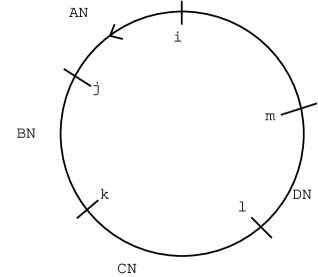
Figure 3.1: Arrangement of nodes for Theorem 6

Let’s follow the slot in the ring that starts out under node $i$ at time 0, and see what packets enter and leave as the slot travels around the ring. What’s the probability that any packet in $i$ at time $t=0$ departs before reaching node $j$? Well, suppose that there’s a packet in $i$. Regardless of the packet’s point of insertion, the probability that it departs in the next $AN$ steps is at least $A$. (If there is no packet in $i$, the event occurs with probability 1.)

Given that the original packet (if any) has departed by node $i$, what’s the probability that a new packet will arrive in that slot by node $j$? If the slot passes under any non-empty queue, it will pick up a packet with probability 1. If not, there’s a probability $p$ of a new arrival on each step. Therefore, the probability of a new packet arriving by node $k$ is at least:

$$1-(1-p)^{BN}=1-\left(1-\frac{2r}{N}\right)^{BN}\rightarrow 1-e^{-2rB}$$

where the limit is taken as $N\rightarrow\infty$.

What’s the probability that this first arrival lasts until node $k$? Well, the earliest it could have arrived is node $i+1$, so the probability is at least $1-A-B=C+D$.

The probability that this packet leaves by node $l$ is $C$, since the latest it could have arrived is node $k$.

The probability that a second packet arrives by node $m$ is $1-e^{-2rD}$, by the same arguments as above.

The chance that this second packet lasts until it reaches node $i$ is $1-C-D=A+B$.

Putting all of these (independent) probabilities together, we find their joint probability is:

$$J=A(A+B)C(C+D)\left(1-e^{-2rB}\right)\left(1-e^{-2rD}\right)$$

The probability of an empty cell arriving at node $i$ is then

$$\frac{1}{(A+B+C+D)N}J+\frac{1}{N}(1-J)$$

(The probability of a packet leaving after one step is always at least $1/N$, which gives the $1/N$ factor in the second term.) Expanding this equation, we get Equation 3.2. $\Box$

We can evaluate the theorem with some fortuitously chosen values.

Corollary 3.3.9.

Set $A=C=.217300$, $B=D=.196640$ in Theorem 3.2. Then for any $\delta>0$, there exists $N_{\delta}$ such that for any $N>N_{\delta}$, the probability of an empty slot arriving at node $i$ at any time after $t=N$ is at least

$$\frac{2}{N}\left[.500026802248-\frac{\delta}{2}\right]$$

We can translate this result into a statement about queue lengths.

Theorem 3.3.10.

Consider a node in any network. Suppose it has Bernoulli arrivals at rate $p$, and the chance that no internal packet arrives at the node is at least $\mu$, independently on every step. Suppose that $\mu>p$, and no more than one internal packet can arrive on each time step. Then the time expected queue length at the node is bounded by

$$\frac{p^{2}(1-\mu)}{\mu(\mu-p)}$$ (3.3)

If this equation (with possibly different values of $p$ and $\mu$) holds at every node in the network, then the network is ergodic.