Stability of Minkowski space in ghost-free massive gravity theory

Abstract

The energy in the ghost-free massive gravity theory is calculated via explicitly resolving the initial value constraints for spherically symmetric deformations of flat space. It turns out that the energy is positive in some cases, but in other cases it can be negative and even unbounded from below. This could suggest that ghost instability is present. However, it seems that the negative energy states cannot communicate with the positive energy sector since the corresponding solutions of the constraint equations are either not globally defined, not asymptotically flat, or singular. As a result, they cannot describe initial data for the decay of flat space. At the same time, for globally regular and asymptotically flat solutions of the constraints the energy is always found to be positive. All of this suggests that there is a physical sector of the theory where the energy is positive and the ghost is suppressed, so that the theory is stable. The negative energies show up only in disjoint sectors and thus should be harmless.

I Introduction

The idea that gravitons could have a tiny mass, which would explain the current cosmic acceleration Perlmutter et al. (1999); *1538-3881-116-3-1009, has attracted a lot of interest after the discovery of the special massive gravity theory by de Rham, Gabadadze, and Tolley (dRGT) de Rham et al. (2011) (see Hinterbichler (2012); *deRham:2014zqa for a review). This theory contains two Hamiltonian constraints which eliminate one propagating degree of freedom (DOF), usually associated with the ghost Hassan and Rosen (2012a); *Kluson:2012wf; *Comelli:2012vz – an unphysical mode with a negative kinetic energy rendering the theory unstable Boulware and Deser (1972). The remaining five DOFs behave well in special limits; hence they are associated with the five polarizations of the massive graviton, and the whole theory is referred to as ghost free.

At the same time, nothing guarantees that removing one DOF kills the ghost completely. It may be that the remaining five DOFs are still contaminated with its remnant, suppressed in some cases but present otherwise. Indeed, such a concern is supported by the observations of certain ghost-type features in the theory De Felice et al. (2012); *Fasiello:2013woa; *Chamseddine:2013lid.

A good way to see whether the theory is indeed ghost free is to compute the energy since, if the energy is positive, the ghost is absent. The energy can be defined in the standard way within the canonical approach Arnowitt et al. (1962), but to evaluate it requires resolving the constraints, which are known, in general, only implicitly. Therefore, the aim of this work is to evaluate the energy in the spherically symmetric sector (the $s$ sector), where the constraints can be obtained explicitly and, in some cases, resolved. The corresponding solutions can be viewed as initial data for the Cauchy problem.

It turns out that the energy is positive in some cases, but in other cases it is negative and unbounded from below. This could suggest that the ghost is still present in the theory. However, a closer inspection reveals that the negative energy states form disjoint branches that cannot communicate with the positive energy sector. Specifically, the corresponding solutions of the constraint equations are either not globally defined, not asymptotically flat, or singular. As a result, they cannot describe initial data for the decay of the flat space. At the same time, for globally regular and asymptotically flat solutions of the constraints, the energy is always found to be positive.

All of this suggests that there is a physical sector of the theory where the energy is positive and the ghost is suppressed, so that the theory is stable. The negative energies show up only in disjoint sectors, so they are harmless. This also suggests that the other seemingly unphysical properties of the theory, like superluminality Deser and Waldron ; *Deser:2013rxa; *Deser:2013eua; *Deser:2013qza; *Deser:2013gpa, may perhaps show up only in disjoint sectors, in which case they would be harmless as well.

II Massive gravity

The theory is defined by the action

$$\frac{1}{M^{2}_{\rm Pl}}S=\int\,\sqrt{-{g}}\left(\frac{1}{2}\,R-{m^{2}}\,{\cal U}\right)\,d^{4}x\equiv\int{\cal L}\,d^{4}x\,.\,$$ (1)

For the generic massive gravity that reduces to the Fierz-Pauli (FP) theory Fierz and Pauli (1939) in the weak field limit, the potential ${\cal U}$ is

$${\cal U}=\frac{1}{8}\,(H^{\mu}_{\leavevmode\nobreak\ \nu}H^{\nu}_{\leavevmode\nobreak\ \mu}-(H^{\mu}_{\leavevmode\nobreak\ \mu})^{2})+\ldots$$ (2)

Here $H^{\mu}_{\leavevmode\nobreak\ \nu}=\delta^{\mu}_{\nu}-g^{\mu\alpha}f_{\alpha\nu}$, where $g^{\mu\nu}$ is the inverse of the spacetime metric, $f_{\mu\nu}$ is the flat metric, and the dots denote terms which are higher order in $H^{\mu}_{\leavevmode\nobreak\ \nu}$ and which can be arbitrary. A particular choice of these terms determines the dRGT theory de Rham et al. (2011), in which case ${\cal U}$ can be expressed as

$${\cal U} = b_{0}+b_{1}\sum_{a}\lambda_{a}+b_{2}\sum_{a<b}\lambda_{a}\lambda_{b}$$ (3)

$$+ b_{3}\sum_{a<b<c}\lambda_{a}\lambda_{b}\lambda_{c}+b_{4}\,\lambda_{0}\lambda_{1}\lambda_{2}\lambda_{3}\,.$$

Here $\lambda_{a}$ are eigenvalues of $\boldsymbol{\gamma}^{\mu}_{\leavevmode\nobreak\ \nu}=\sqrt{{{g}}^{\mu\alpha}{{f}}_{\alpha\nu}}$, with the square root understood in the sense that $\boldsymbol{\gamma}^{\mu}_{\leavevmode\nobreak\ \alpha}\boldsymbol{\gamma}^{\alpha}_{\leavevmode\nobreak\ \nu}={{g}}^{\mu\alpha}{{f}}_{\alpha\nu}.$ If the bare cosmological term is absent, the flat space is a solution of the theory, and $m$ in (1) is the FP mass of the graviton in the weak field limit, then the parameters $b_{k}$ are expressed in terms of two arbitrary $c_{3},c_{4}$ as $b_{0}=4c_{3}+c_{4}-6$, $b_{1}=3-3c_{3}-c_{4}$, $b_{2}=2c_{3}+c_{4}-1$, $b_{3}=-c_{3}-c_{4}$, and $b_{4}=c_{4}$.

III Hamiltonian in the $S$ sector

Assuming the spherical coordinates $x^{\mu}=(t,r,\vartheta,\varphi)$, the two metrics can be parametrized as

$$ds_{g}^{2} = -N^{2}dt^{2}+\frac{1}{\Delta^{2}}(dr+\beta\,dt)^{2}+R^{2}\,(d\vartheta^{2}+\sin^{2}\vartheta d\varphi^{2}),$$

$$ds_{f}^{2} = -dt^{2}+dr^{2}+r^{2}\,(d\vartheta^{2}+\sin^{2}\vartheta d\varphi^{2}),$$ (4)

where $N,\beta,\Delta$, and $R$ depend on $t$ and $r$. Defining the canonical momenta $p_{\Delta}={\partial\cal L}/{\partial\dot{\Delta}}$ and $p_{R}={\partial\cal L}/{\partial\dot{R}}$ and introducing ${\cal V}=\sqrt{-g}\,{\cal U}$, the Hamiltonian density is

$${\cal H} = \dot{\Delta}\pi_{\Delta}+\dot{R}\pi_{R}-{\cal L}=N{\cal H}_{0}+\beta{\cal H}_{r}+{m^{2}}{\cal V},\leavevmode\nobreak\ \leavevmode\nobreak\ \leavevmode\nobreak\$$ (5)

where the total derivative has been omitted, and

$${\cal H}_{0} = \frac{\Delta^{3}}{4R^{2}}\,p_{\Delta}^{2}+\frac{\Delta^{2}}{2R}\,p_{\Delta}p_{R}+\Delta R^{\prime 2}+2R(\Delta R^{\prime})^{\prime}-\frac{1}{\Delta}\,,\leavevmode\nobreak\ \leavevmode\nobreak\ \leavevmode\nobreak\ \leavevmode\nobreak\ \leavevmode\nobreak\$$

$${\cal H}_{r} = \Delta p_{\Delta}^{\prime}+2\Delta^{\prime}p_{\Delta}+R^{\prime}p_{R}\,.$$ (6)

These expressions were studied previously in Unruh (1976); *Kuchar:1994zk. The phase space is spanned by four variables $(q^{i},p_{k})\equiv\{\Delta,R,p_{\Delta},p_{R}\}$, while $N$ and $\beta$ are nondynamical since their momenta vanish.

General Relativity is recovered for $m=0$, in which case varying ${\cal H}$ with respect to $N$ and $\beta$ gives 2 constraints: ${\cal H}_{0}=0$ and ${\cal H}_{r}=0$. They are first class and generate diffeomorphisms, which can be used to impose two gauge conditions. As a result, there remain $4-2-2=0$ independent phase space variables; therefore there is no dynamics in the $s$ sector (the Birkhoff theorem). The energy vanishes on the constraint surface (up to the surface term Regge and Teitelboim (1974)).

If $m\neq 0$, then varying ${\cal H}$ with respect to $N$ and $\beta$ gives

$${\cal H}_{0}+m^{2}\frac{\partial\cal V}{\partial N}=0,\leavevmode\nobreak\ \leavevmode\nobreak\ \leavevmode\nobreak\ \leavevmode\nobreak\ \leavevmode\nobreak\ {\cal H}_{r}+m^{2}\frac{\partial\cal V}{\partial\beta}=0.\leavevmode\nobreak\ \leavevmode\nobreak\$$ (7)

For the generic potential (2), these relations can be resolved to express $N$ and $\beta$ in terms of $(q^{i},p_{k})$. No constraints then arise, so that all four phase space variables are independent and they describe two DOFs. One of them can be interpreted as the scalar polarization of the massive graviton, while the second one must be the ghost. Inserting $N(q^{i},p_{k})$ and $\beta(q^{i},p_{k})$ into ${\cal H}$, the result is not positive definite. In particular, the kinetic part of the energy associated with the momenta can be negative and arbitrarily large, which produces ghost instability Boulware and Deser (1972).

In the dRGT theory, one has

$${\cal V}=\frac{NR^{2}P_{0}}{\Delta}+\frac{R^{2}P_{1}}{\Delta}\,\sqrt{(\Delta N+1)^{2}-\beta^{2}}+R^{2}P_{2}\,,$$ (8)

with $P_{n}=b_{n}+2b_{n+1}\,{r}/{R}+b_{n+2}\,{r^{2}}/{R^{2}}.$ The second relation in (7) then determines the shift $\beta$,

$$\beta=(N\Delta+1)\frac{\Delta{\cal H}_{r}}{Y}\,,$$ (9)

where $Y\equiv\sqrt{(\Delta{\cal H}_{r})^{2}+({m^{2}}R^{2}P_{1})^{2}}\,.$ Inserting this into the first relation in (7) does not, however, determine the lapse $N$, but gives a constraint,

$${\cal C}\equiv{\cal H}_{0}+Y+{m^{2}}\frac{R^{2}P_{0}}{\Delta}=0.$$ (10)

Inserting (9) into (5) yields ${\cal H}={\cal E}+N{\cal C},$ with

$${\cal E} = \frac{Y}{\Delta}+{m^{2}}R^{2}P_{2}\,,$$ (11)

so that varying ${\cal H}$ with respect to $N$ reproduces the constraint equation ${\cal C}=0$ once again. Since the constraint should be preserved in time, its Poisson bracket $\{,\}_{\rm PB}$ Hassan and Rosen (2012a); *Kluson:2012wf; *Comelli:2012vz with the Hamiltonian ${H}=\int_{0}^{\infty}{\cal H}\,dr$ should vanish. One can check that $\{{\cal C}(r_{1}),{\cal C}(r_{2})\}_{\rm PB}=0;$ therefore ${\cal S}\equiv\{{\cal C},{H}\}_{\rm PB}=0$ is a new constraint since the term proportional to $N$ drops out of the bracket. Explicitly,

$${\cal S} = \frac{m^{4}R^{2}P_{1}^{2}}{2Y}\,(\Delta p_{\Delta}+R\,p_{R})-Y\left(\frac{\Delta{\cal H}_{r}}{Y}\right)^{\prime}$$ (12)

$$- \frac{\Delta^{2}p_{\Delta}}{2R}\left\{\frac{m^{4}}{2\Delta Y}\,\partial_{R}(R^{4}P_{1}^{2})+m^{2}\partial_{R}(R^{2}P_{2})\right\}$$

$$- \frac{m^{2}{\cal H}_{r}}{Y}\left\{\Delta^{2}\left(R^{2}P_{2}\right)^{\prime}+R^{2}\partial_{r}(P_{0}-\Delta^{2}P_{2})\right\}\,,$$

where ${}^{\prime}\equiv d/dr$ and $\partial_{R}$ and $\partial_{r}$ are the partial derivatives with respect to $R$ and $r$. It is worth noting that the two constraints have been known up to now only implicitly Hassan and Rosen (2012a); *Kluson:2012wf; *Comelli:2012vz, whereas Eqs.(10) and (12) provide explicit expressions for any values of the parameters $b_{k}$. Requiring further that $\{{\cal S},{H}\}_{\rm PB}=0$ yields an equation for $N$ because $\{{\cal C},{\cal S}\}_{\rm PB}\neq 0,$ the term containing $N$ does not drop out.

Since the constraints are second class, they remove one of the two DOFs in the $s$ sector. It is not immediately obvious which one is removed, but if the energy is positive, it follows that it is the ghost which is removed.

The energy is $E=\int_{0}^{\infty}{\cal E}\,dr\,,$ where the arguments of ${\cal E}$ should fulfill two constraint equations: ${\cal C}=0$ and ${\cal S}=0$. These are nonlinear differential equations whose solutions $\Delta,R,p_{\Delta}$, and $p_{R}$ can be viewed as initial data for the Cauchy problem at the moment $t=0$. These equations are complicated, but they simplify in some cases.

IV Weak field limit

In flat space, where $N=\Delta=1$, $R=r$, and $\beta=p_{\Delta}=p_{R}=0$, one has ${\cal C}={\cal S}={\cal E}=0$. If deviations from flat space are small, then ${\cal C}={\cal C}_{\rm FP}+\ldots$ and ${\cal S}={\cal S}_{\rm FP}+\ldots$ (where the dots denote higher order terms), while the leading terms are, with $\delta\equiv\Delta-1$ and $\rho\equiv R-r$,

$${\cal C}_{\rm FP}=(2r(\delta+\rho^{\prime}))^{\prime}+m^{2}(r^{2}\delta-2r\rho),$$

$${\cal S}_{\rm FP}=\frac{m^{2}}{2}\,(rp_{R}-p_{\Delta})-(p_{\Delta}^{\prime}+p_{R})^{\prime}.$$ (13)

If $\nu\equiv N-1$, then ${\cal H}={\cal E}_{\rm FP}+\nu\,{\cal C}_{\rm FP}+\ldots$, where ${\cal E}_{\rm FP}$ is the leading (up to a total derivative) part of ${\cal E}+{\cal C}$,

$${\cal E}_{\rm FP} = \frac{p_{\Delta}^{2}}{4r^{2}}+\frac{p_{\Delta}p_{R}}{2r}+\frac{(p_{\Delta}^{\prime}+p_{R})^{2}}{m^{2}r^{2}}\,$$ (14)

$$+ 2\rho\,\delta^{\prime}-\rho^{\prime 2}-\delta^{2}+m^{2}(2r\delta\rho-\rho^{2}).$$

These are the FP constraints and the energy density. The constraints are solved by

$$\delta = -\rho^{\prime}+\frac{Q^{\prime}}{r^{2}},\leavevmode\nobreak\ \leavevmode\nobreak\ \leavevmode\nobreak\ \leavevmode\nobreak\ \leavevmode\nobreak\ \leavevmode\nobreak\ \rho=\frac{Q}{r^{2}}+\frac{2Q^{\prime}}{m^{2}r^{3}},$$

$$p_{R} = -p_{\Delta}^{\prime}+\frac{F^{\prime}}{r},\leavevmode\nobreak\ \leavevmode\nobreak\ \leavevmode\nobreak\ \leavevmode\nobreak\ \leavevmode\nobreak\ \leavevmode\nobreak\ p_{\Delta}=\frac{F}{r}-\frac{2F^{\prime}}{m^{2}r^{2}}\,$$ (15)

for arbitrary $Q(r)$ and $F(r)$. Inserting this into (14) gives

$${\cal E}_{\rm FP}=\frac{3}{r^{4}}\left(Q^{\prime 2}+m^{2}Q^{2}+\frac{F^{2}}{4}\right)+\left(\ldots\right)^{\prime}.$$ (16)

Since the fields should be weak, all of the above functions should be bounded, which imposes certain fall-off conditions on $Q$ and $F$ at the origin and at infinity. These conditions imply that the total derivative term in (16) vanishes upon integration; therefore the energy is positive.

V Momentum sector

Let us assume that the three-metric is flat, so that $\Delta=1$ and $R=r$, while the momenta $p_{\Delta}$ and $p_{R}$ are not necessarily small and satisfy the two constraint equations (10) and (12). Introducing the dimensionless radial coordinate $x=mr$ with ${}^{\prime}\equiv d/dx$, expressing the two momenta in terms of two new function, $z$ and $f$, as

$$p_{\Delta}=\frac{\sqrt{xz}}{m}\,,\leavevmode\nobreak\ \leavevmode\nobreak\ \leavevmode\nobreak\ \leavevmode\nobreak\ p_{R}=-\frac{(xz+4x^{4}f)}{2x\sqrt{xz}}\,,$$ (17)

the constraints reduce to two equations,

$$z^{\prime} = 4\,x^{2}f+2x\sqrt{xz}\,F\,,$$ (18)

$$f^{\prime} = \frac{4\,(1-c_{3})\,zf-4x^{3}f-3z}{4x\sqrt{xz}}\,F-\frac{2}{x}\,F^{2}\,,$$

with $F=\pm\sqrt{f(f+2)}$, while the energy density ${\cal E}=x^{2}f\,.$ Since $F^{2}=f(f+2)\geq 0$, this implies that either one has $f\geq 0$ or $f\leq-2$, which determines two different solution branches whose energy is either non-negative or strictly negative. There can be no interpolation between the branches, since this would require crossing the region of forbidden values of $f$.

A simple solution from the first branch is $f=0$ and $z=z_{0}$, whose energy is zero. It reduces to the flat space configuration for $z_{0}=0$. If the solutions of Eq.(18) are to describe initial values for perturbations around flat space, then they should correspond to smooth deformations of the latter, and this selects the $f\geq 0$ branch. Therefore, the energy for perturbations around flat space is positive.

A simple solution from the second branch is $f=-2$ and $z=\frac{8}{3}\,(x_{\rm max}^{3}-x^{3})$, where $x_{\rm max}$ is an integration constant. Since $z$ should be positive, the solution exists only for $x\leq x_{\rm max}$, with the total energy $E=\int{\cal E}\,dr=-\frac{2}{3m}\,x_{\rm max}^{3}$. One can construct more general negative energy solutions of Eq.(18) numerically. They exist only within finite intervals of $x$ at whose ends one has either $f\to-\infty$ or $z\to 0$. Such solutions cannot describe regular initial data and they belong to the disjoint from flat space branch.

Summarizing, the energy of smooth excitations over the flat space is positive. It can also be negative, but only in a sector disconnected from flat space; therefore this cannot lead to the ghost instability of the latter.

VI Metric sector

Let us now set the momenta to zero, $p_{\Delta}=p_{R}=0$, without fixing $\Delta$ and $R$. This solves the second constraint, ${\cal S}=0.$ Denoting $h=R/r$ and $g=\Delta h$, using again $x=mr$ with ${}^{\prime}\equiv d/dx$, and setting $c_{3}=c_{4}=0$ for simplicity, the first constraint reduces to

$$h^{\prime\prime}+\frac{2}{x}\,h^{\prime}-\frac{h^{\prime 2}}{2h}+\frac{(xh)^{\prime}g^{\prime}}{xg}-\frac{h(1-g^{2})}{2x^{2}g^{2}}$$ (19)

$$- \frac{h(2-3h)}{2g}-\frac{h(1-6h+6h^{2})}{2g^{2}}=0,$$

and the energy density

$${\cal E} = \frac{x^{2}h^{2}(3h-g-2)}{g}\,.$$ (20)

The constraint is solved by setting $g=qh/(xh)^{\prime}$ and

$$Q = xh(1-q^{2})+x^{3}h(h-1)(2h-1),$$

$$Q^{\prime} = x^{2}h(q-1)(3h-2),$$ (21)

with any $Q(x)$. Having chosen $Q$, these algebraic equations can be resolved with respect to $h$ and $q$. Even though the second constraint is trivially satisfied, its stability condition, $\{{\cal S},H\}_{\rm PB}=0$, is nontrivial, ${\cal A}N-{\cal B}=0\,,$ with

$${\cal A} = q(\alpha_{1}+\alpha_{2})+2(q-1)^{2}(27h^{2}-18h+4)(xh)^{\prime}$$ (22)

$$- 6x^{2}h(3h-1)(3h-2)(4h-3)(xh)^{\prime},$$

$${\cal B} = (\alpha_{2}-\alpha_{1})(xh)^{\prime}+8h^{2}q(q-1)^{2}+6h^{2}x^{2}q(3h-2)^{2}\,,$$

where $\alpha_{1}=3x^{2}h(3h-2)(13h^{2}-12h+2)$ and $\alpha_{2}=2h(q-1)^{2}(9h-2)$. Thus the lapse function is $N={\cal B}/{\cal A}$, while the shift function obtained from Eq.(9) is $\beta=0$.

The three-metric will be regular and asymptotically flat if $h$ and $q$ are smooth and fulfill the boundary conditions

$$h_{0}\leftarrow h\to 1,\leavevmode\nobreak\ \leavevmode\nobreak\ 1\leftarrow q\to 1\leavevmode\nobreak\ \leavevmode\nobreak\ \leavevmode\nobreak\ \leavevmode\nobreak\ \leavevmode\nobreak\ \mbox{for}\leavevmode\nobreak\ \leavevmode\nobreak\ 0\leftarrow x\to\infty,$$ (23)

with $h_{0}>0$. The simplest solutions of the constraint are obtained by setting in (VI) $Q=0$, which implies that $q=1$, but yields two different solutions for $h$:

$$h(x)=\left\{1,\frac{1}{2}\right\}\leavevmode\nobreak\ \leavevmode\nobreak\ \leavevmode\nobreak\ \leavevmode\nobreak\ \Rightarrow\leavevmode\nobreak\ \leavevmode\nobreak\ \leavevmode\nobreak\ \leavevmode\nobreak\ \leavevmode\nobreak\ {\cal E}(x)=\left\{0,-\frac{3}{8}\,x^{2}\right\}.$$ (24)

These fulfill also the Hamilton equations, $\dot{q}_{k}=\{q_{k},H\}_{\rm PB}=0$ and $\dot{p}_{k}=\{p_{k},H\}_{\rm PB}=0$, and give rise to two different branches of more general solutions of the constraint.

VI.1 Normal branch

For the $h=1$ solution in (24), one has $N=1$, so that the four-metric is flat, $ds_{g}^{2}=\,ds_{f}^{2}$, and the energy is zero. For deformations of this solution, one has $h=h_{0}+{\cal O}(x^{2})$ and $q=1+{\cal O}(x^{2})$ for small $x$, in which case Eqs.(19) and (VI) require that $Q=kr^{5}+{\cal O}(x^{7})$ with $k=0.1\times h_{0}(2h_{0}-1)(h_{0}-1)(3h_{0}-2)$. This suggests that one can choose $Q=kr^{5}/(1+Ax^{2}e^{x})$, and resolving Eq.(VI) with respect to $h$ and $q$ then gives the global solutions shown in Fig.1.

   

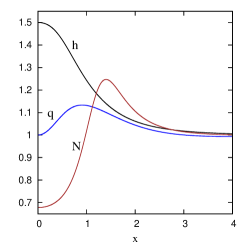
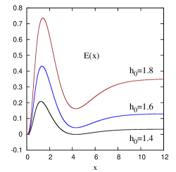
Figure 1: Profiles of $h,q,N$, and $E(x)$ for the positive energy solutions with $Q=kr^{5}/(1+x^{2}e^{x})$.

These solutions are smooth and globally regular; they describe initial metric deformations of flat space. Interestingly, the energy (expressed in $1/m$ units) contained in the sphere or radius $x$, $E(x)=\int_{0}^{x}{\cal E}\,dx,$ can be negative for small $x$ (if $h_{0}<1$), but the total energy $E(\infty)$ is always positive and grows when $|h_{0}-1|$ increases. As a result, the energy is positive for smooth, asymptotically flat fields, so that the positivity of their energy in the weak field limit holds in the fully nonlinear theory as well.

VI.2 Tachyon branch

For the $h=\frac{1}{2}$ solution in (24), one has $N=\frac{1}{2}$, so that the metrics are proportional, $ds_{g}^{2}=\frac{1}{4}\,ds_{f}^{2}$. Even though they are both flat, this solution is quite different from flat space since one now has $E(x)=-x^{3}/8$, which corresponds to the constant negative energy density. The total energy is negative and infinite. Considering small fluctuations around this background, the corresponding Fierz-Pauli mass is $m_{\rm FP}^{2}=-\frac{1}{2}\,m^{2}$ [as is seen by linearizing the constraints and comparing with (IV)], hence gravitons become tachyons, which can be viewed as an indication of the presence of the ghost.

One can also construct more general solutions of this type by setting in (23) $h_{0}\approx\frac{1}{2}$, in which case $h(x)\to\frac{1}{2}$ as $x\to\infty$. The energy is always negative and infinite. However, none of these solutions fulfill the boundary condition (23). Since they are not asymptotically flat, they cannot affect the stability of flat space.

VI.3 Tachyon bubbles

There are also asymptotically flat solutions whose energy is finite and negative. They can be obtained by choosing in (VI) $Q=A\,\Theta(x-x_{0})(x-x_{0})^{p}e^{-x}$, where $\Theta(x)$ is the step function. This enforces for $h$ a kink-type behavior, so that $h=\frac{1}{2}$ for $x<x_{0}$, but $h$ increases for $x>x_{0}$ and approaches unity as $x\to\infty$ (see Fig.2). Solutions thus approach the flat space at infinity, but they contain a bubble of the tachyon phase in a finite region. If $x_{0}$ is large, then the energy $E\propto-x_{0}^{3}$ (see Fig.2). The existence of such solutions is embarrassing, since it suggests that the flat space could be unstable with respect to decay into bubbles.

   

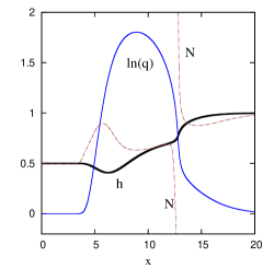
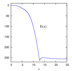
Figure 2: Profiles of $h$ (thick line), $\ln(q)$, $N$, and $E(x)$ for the tachyon bubble solution with $Q=-\Theta(x-3)(x-3)^{8}e^{-x}$.

However, a closer inspection reveals that the lapse function $N$ for the bubbles is singular. Indeed, one has $N={\cal B}/{\cal A}$, but both ${\cal A}$ and ${\cal B}$ have opposite signs for $h=\frac{1}{2}$ and $h=1$; hence they vanish at least once as $h$ interpolates between $\frac{1}{2}$ and $1$. One can show that they cannot vanish simultaneously; therefore $N$ must have at least one zero and a pole, as shown in Fig.2. Since $N$ enters the Hamilton equations $\dot{p}_{k}=\{p_{k},H\}_{\rm PB}$, the time derivative of the momenta diverges where $N$ has pole(s). Therefore, the bubble solutions do not describe regular initial data, so that they cannot provoke instability of flat space. The tachyon bubbles can be obtained also for other values of the theory parameters $c_{3}$ and $c_{4}$, but their lapse function $N$ is always found to be singular.

VII Stability of the theory

To recapitulate, the above results indicate that the energy in the dRGT theory is positive for globally regular and asymptotically flat fields. The energy can also be negative and even unbounded from below, but in all studied cases the corresponding solutions are found to be either not asymptotically flat or not global or singular. They cannot describe initial data for a decay of the flat space. Therefore, one is bound to conclude that there is evidence for the stability of flat space, despite the existence of the negative energies.

One can provide the following interpretation. Globally regular and asymptotically flat fields constitute the “physical sector” of the theory where the energy is positive and the ghost is absent/bound. One may hope that a positive energy theorem can be proven in this case. As for the negative energy states, they belong to disjoint sectors and cannot communicate with the physical sectors since they are singular. Therefore, even though the negative energies can be viewed as an unphysical feature, they are harmless because they decouple.

One may wonder if these classical arguments could be extended to show that the physical sector is protected against quantum corrections. Let us estimate the height of the potential barrier between the different sectors. This can be done by computing the energy for interpolating sequences of fields. For example, fields which fulfill the constraint and satisfy the boundary conditions (23) will interpolate between the normal and tachyon branches when the parameter $h_{0}$ in (23) decreases from $1$ to $1/2$. It turns out that when $h_{0}$ starts decreasing, the energy rapidly grows, since the function $g$ in the denominator in (20) develops a minimum (the lapse function $N$ then typically shows several poles). As $h_{0}$ continues to decrease, the energy passes through a simple pole and then approaches a finite negative value when $h_{0}$ tends to $1/2$. Therefore, the potential barrier between the two branches is infinitely high.

However, it is still possible that the barrier height could be made finite via minimizing the energy with respect to the function $Q(x)$ in (VI). Let us suppose that the minimal barrier height indeed has a finite value, $E_{b}>0$. This value cannot be arbitrarily small, since when one starts deviating from flat space the energy grows, because the Fierz-Pauli energy is positive. Therefore, the energy can show a maximum and start decreasing only when the nonlinear effects become essential, but by this moment it should already assume a finite value. The dimensionful energy is obtained by dividing by the graviton mass, $E_{\rm b}/m$, and since $m$ is extremely small, the energy will be extremely large, of the order of the total energy contained in our Universe. As a result, even if the potential barrier between different sectors was finite, it would be cosmologically large, implying that the physical sector should actually be stable both classically and quantum mechanically.

It is also worth noting that within the bigravity generalization of the dRGT theory where both metrics are dynamical Hassan and Rosen (2012b), the tachyon vacuum in (24) is no longer a solution, as it does not fulfill the equations for the second metric. Therefore, since there are less negative energy solutions, it seems that the positivity of the energy should be easier to demonstrate when both metrics are dynamical. Similarly, including a matter source should also have a stabilizing effect since the energy of the physical matter is expected to be positive.

The decoupling of the negative energies suggests that the other seemingly unphysical features of the dRGT theory, such as the superluminality Deser and Waldron ; *Deser:2013rxa; *Deser:2013eua; *Deser:2013qza; *Deser:2013gpa, may also decouple. In fact, it has not been shown that the superluminality should inevitably develop starting from any smooth initial data. On the contrary, one could expect different unphysical features to come up together, so that superluminal fields can be expected to have negative energies. But then they should decouple. Although not a proof, this indicates that the superluminality could perhaps relate only to the unphysical sectors, in which case it would be harmless.

VIII Acknowledgments

It is a pleasure to acknowledge discussions with Claudia de Rham, Andrew Tolley, and Cedric Deffayet and interesting remarks of Eugeny Babichev. This work was partly supported by the Russian Government Program of Competitive Growth of the Kazan Federal University.

References

- Perlmutter et al. (1999) S. Perlmutter et al., Astrophys.Journ. 517, 565 (1999).
- Riess et al. (1998) A. Riess et al., Astron.Journ. 116, 1009 (1998).
- de Rham et al. (2011) C. de Rham, G. Gabadadze, and A. Tolley, Phys.Rev.Lett. 106, 231101 (2011).
- Hinterbichler (2012) K. Hinterbichler, Rev.Mod.Phys. 84, 671 (2012).
- de Rham (2014) C. de Rham, (2014), arXiv:1401.4173 [hep-th] .
- Hassan and Rosen (2012a) S. Hassan and R. A. Rosen, JHEP 1204, 123 (2012a).
- Kluson (2012) J. Kluson, Phys.Rev. D86, 044024 (2012).
- Comelli et al. (2012) D. Comelli, M. Crisostomi, F. Nesti, and L. Pilo, Phys.Rev. D86, 101502 (2012).
- Boulware and Deser (1972) D. Boulware and S. Deser, Phys.Rev. D6, 3368 (1972).
- De Felice et al. (2012) A. De Felice, E. Gumrukcuoglu, and S. Mukohyama, Phys.Rev.Lett. 109, 171101 (2012).
- Fasiello and Tolley (2013) M. Fasiello and A. J. Tolley, JCAP 1312, 002 (2013).
- Chamseddine and Mukhanov (2013) A. H. Chamseddine and V. Mukhanov, JHEP 1303, 092 (2013).
- Arnowitt et al. (1962) R. L. Arnowitt, S. Deser, and C. W. Misner, in Gravitation: An Introduction to Current Research, edited by Louis Witten (Wiley, 1962) Chap. 7, pp. 227–265, gr-qc/0405109 .
- (14) S. Deser and A. Waldron, Phys.Rev.Lett. 110, 111101.
- Deser and Waldron (2014) S. Deser and A. Waldron, Phys.Rev. D89, 027503 (2014).
- Deser et al. (2013a) S. Deser, K. Izumi, Y. Ong, and A. Waldron, Phys.Lett. B726, 544 (2013a).
- Deser et al. (2013b) S. Deser, K. Izumi, Y. Ong, and A. Waldron, (2013b), arXiv:1312.1115 [hep-th] .
- Deser et al. (2013c) S. Deser, M. Sandora, and A. Waldron, Phys.Rev. D88, 081501 (2013c).
- Fierz and Pauli (1939) M. Fierz and W. Pauli, Proc.Roy.Soc.Lond. A173, 211 (1939).
- Unruh (1976) W. Unruh, Phys.Rev. D14, 870 (1976).
- Kuchar (1994) K. V. Kuchar, Phys.Rev. D50, 3961 (1994).
- Regge and Teitelboim (1974) T. Regge and C. Teitelboim, Annals Phys. 88, 286 (1974).
- Hassan and Rosen (2012b) S. Hassan and R. A. Rosen, JHEP 1202, 126 (2012b).