$R$-Dimensional ESPRIT-Type Algorithms for Strictly Second-Order Non-Circular Sources and Their Performance Analysis

Abstract

High-resolution parameter estimation algorithms designed to exploit the prior knowledge about incident signals from strictly second-order (SO) non-circular (NC) sources allow for a lower estimation error and can resolve twice as many sources. In this paper, we derive the $R$-D NC Standard ESPRIT and the $R$-D NC Unitary ESPRIT algorithms that provide a significantly better performance compared to their original versions for arbitrary source signals. They are applicable to shift-invariant $R$-D antenna arrays and do not require a centro-symmetric array structure. Moreover, we present a first-order asymptotic performance analysis of the proposed algorithms, which is based on the error in the signal subspace estimate arising from the noise perturbation. The derived expressions for the resulting parameter estimation error are explicit in the noise realizations and asymptotic in the effective signal-to-noise ratio (SNR), i.e., the results become exact for either high SNRs or a large sample size. We also provide mean squared error (MSE) expressions, where only the assumptions of a zero mean and finite SO moments of the noise are required, but no assumptions about its statistics are necessary. As a main result, we analytically prove that the asymptotic performance of both $R$-D NC ESPRIT-type algorithms is identical in the high effective SNR regime. Finally, a case study shows that no improvement from strictly non-circular sources can be achieved in the special case of a single source.

I Introduction

Estimating the parameters of multidimensional ($R$-D) signals with $R\geq 1$, e.g., their directions of arrival, frequencies, Doppler shifts, etc., has long been of great research interest, given its importance in a variety of applications such as radar, sonar, channel sounding, and wireless communications. Among other subspace-based parameter estimation schemes (see [1, 2]), $R$-D Standard ESPRIT [3], $R$-D Unitary ESPRIT [4, 5], and their tensor extensions $R$-D Standard Tensor-ESPRIT and $R$-D Unitary Tensor-ESPRIT [6] are some of the most valuable estimators due to their high resolution and their low complexity. However, these methods assume arbitrary source signals and do not take prior knowledge such as the second-order (SO) non-circularity of the received signals into account. With the growing popularity of subspace-based parameter estimation algorithms, their performance analysis has attracted considerable attention. The two most prominent performance assessment strategies have been proposed in [7] and [8]. The concept in [7] and the follow-up papers [9, 10, 11] analyze the eigenvector distribution of the sample covariance matrix, originally proposed in [12]. However, it requires Gaussianity assumptions on the source symbols and the noise, and is only asymptotic in the sample size $N$. In contrast, [8] and its extensions [13, 14] provide an explicit first-order approximation of the estimation error caused by the perturbed subspace estimate due to a small additive noise contribution. It directly models the leakage of the noise subspace into the signal subspace. Unlike [7], this approach is asymptotic in the effective signal-to-noise ratio (SNR), i.e., the results become accurate for either high SNRs or a large sample size $N$. Thus, it is even valid for the single snapshot case $N=1$ if the SNR is sufficiently high. Furthermore, as it is explicit in the noise realizations, no assumptions about the statistics of the signals or the noise are necessary. However, for the mean squared error (MSE) expressions in [8], a circularly symmetric noise distribution is assumed. In [15] and [16], we have derived new MSE expressions that only require the noise to be zero-mean with finite SO moments regardless of its statistics and extended the framework of [8] to the case of $R$-D parameter estimation. Further extensions of these results for the perturbation analyses of Tensor-ESPRIT-type algorithms have been presented in [17] and [18], respectively. The special case of the performance assessment for a single source was considered in [7] and the asymptotic efficiency of MUSIC and Root-MUSIC was presented in [19] and [20], respectively. However, these results are asymptotic in the sample size $N$ or even in the number of sensors $M$. The results presented here are also accurate for small values of $M$ and asymptotic in the effective SNR.

Recently, a number of improved high-resolution subspace-based parameter estimation schemes have been proposed for strictly non-circular (NC) sources. These include NC MUSIC [21], NC Root-MUSIC [22], 1-D NC Standard ESPRIT [23], and 2-D NC Unitary ESPRIT [24]. Unlike the original parameter estimation methods, they exploit prior knowledge about the signals’ SO statistics, i.e., their strict SO non-circularity [25]. Examples of such signals include BPSK, Offset-QPSK, PAM, and ASK-modulated signals. By applying a preprocessing procedure similar to the concept of widely-linear processing [25], the array aperture is virtually doubled, which results in a significantly reduced estimation error and the ability to resolve twice as many sources [24]. Some potential applications are wireless communications, cognitive radio, etc., when strictly non-circular sources are known to be present, and radar, tracking, channel sounding, etc., where the signals can be designed as strictly non-circular signals. The performance of NC MUSIC has been derived in [21] based on [7], its source resolvability has been investigated in [26], and mutual coupling has been considered in [27]. However, a performance analysis of NC Standard ESPRIT and NC Unitary ESPRIT has not yet been reported in the literature.

In this paper, we first present the $R$-D NC Standard ESPRIT and the $R$-D NC Unitary ESPRIT algorithms as an extension of [23] and [24]. They exploit the strict SO non-circularity of stationary sources. The algorithms in [23] and [24] are only designed for the case of 1-D parameter estimation and require a shift-invariant and centro-symmetric array structure. Here, we relax this requirement to only shift-invariant-structured arrays and additionally consider the case of $R$-D ($R\geq 1$) parameter estimation. Furthermore, we show that the preprocessing step for non-circular sources automatically includes forward-backward averaging (FBA) [28], which is in this case even applicable to arrays without centro-symmetry. In analogy to [4], $R$-D NC Unitary ESPRIT can also be efficiently implemented in terms of only real-valued computations by mapping the centro-Hermitian FBA-processed measurement matrix into a real-valued matrix [29]. This substantially reduces the computational complexity. Regarding the estimation error, $R$-D NC Unitary ESPRIT performs better than $R$-D NC Standard ESPRIT at low signal-to-noise ratios (SNR), while simultaneously requiring a lower computational load. Both algorithms achieve a significantly lower estimation error than their traditional (non-NC) counterparts $R$-D Standard ESPRIT and $R$-D Unitary ESPRIT [5].

In our second contribution, we extend our initial results in [30] and derive a first-order asymptotic performance analysis of the proposed $R$-D NC Standard and $R$-D NC Unitary ESPRIT algorithms. Least squares (LS) is used to solve the resulting augmented shift invariance equations after the preprocessing for non-circular sources. Due to its discussed advantages, we resort to the framework in [8] combined with [16] for our presented performance analysis. We further extend [16] by incorporating the preprocessing for non-circular sources and derive an explicit first-order expansion of the estimation error in terms of the noise perturbation. The noise is assumed to be small compared to the signals but no assumptions about its statistics are required. We also provide MSE expressions, where only the assumptions of a zero mean and finite SO moments of the noise are needed. Thus, they also give insights into the achievable performance in scenarios with non-Gaussian and non-circular perturbations that can, for instance, be caused by clutter environments in radar applications [31]. All the obtained expressions are asymptotic in the effective SNR, i.e., they become accurate for either high SNRs or large sample sizes. Furthermore, we analytically prove that $R$-D NC Standard ESPRIT and $R$-D NC Unitary ESPRIT have the same asymptotic performance in the high effective SNR regime. In contrast to [30], we here also take the real-valued transformation in $R$-D NC Unitary ESPRIT into account for the proof.

Finally, we present simplified $R$-D MSE expressions for both NC ESPRIT-type algorithms in the special case of a single strictly non-circular source, where a uniform sampling grid and circularly symmetric white noise are assumed. The obtained closed-form expressions only depend on the physical parameters, i.e., the array size $M$ and the effective SNR. They facilitate design decisions on $M$ to achieve a certain performance for specific SNRs. Furthermore, we also simplify the deterministic $R$-D NC Cramér-Rao bound (CRB) [32] for this case and analytically compute the asymptotic efficiency of the proposed algorithms for $R=1$. Note that in [33] and [34], we have also incorporated structured least squares and spatial smoothing into the performance analysis, respectively.

This remainder of this paper is organized as follows: The data model and the preprocessing for strictly non-circular sources are introduced in Section II and Section III. In Section IV, the $R$-D NC Standard ESPRIT and $R$-D NC Unitary ESPRIT algorithms are derived. Their performance analysis is presented in Section V before the special case of a single source is analyzed in Section VI. Section VII illustrates and discusses the numerical results, and concluding remarks are drawn in Section VIII.

Notation: We use italic letters for scalars, lower-case bold-face letters for column vectors, and upper-case bold-face letters for matrices. The superscripts ^T, ^∗, ^H, ^-1, and ⁺ denote the transposition, complex conjugation, conjugate transposition, matrix inversion, and the Moore-Penrose pseudo inverse of a matrix, respectively. The Kronecker product is denoted as $\otimes$ and the Hadamard product is defined as $\odot$. The operator $\mathop{{\rm vec}}\left\{\bm{A}\right\}$ stacks the columns of the matrix $\bm{A}\in\mathbb{C}^{M\times N}$ into a column vector of length $MN\times 1$ and $\mathrm{arg}\{\cdot\}$ extracts the phase of a complex number. The operator $\mathrm{diag}\{\bm{a}\}$ returns a diagonal matrix with the elements of $\bm{a}$ placed on its diagonal and $\mathrm{blkdiag}\{\cdot\}$ creates a block diagonal matrix. The operator $\mathcal{O}\{\cdot\}$ denotes the highest order with respect to a parameter. The matrix $\bm{\Pi}_{M}$ is the $M\times M$ exchange matrix with ones on its antidiagonal and zeros elsewhere. Also, the matrices $\bm{1}_{M}$ and $\bm{0}_{M}$ denote the $M\times M$ matrices of ones and zeros, respectively. Moreover, $\mathop{{\rm Re}}\left\{\cdot\right\}$ and $\mathop{{\rm Im}}\left\{\cdot\right\}$ extract the real and imaginary part of a complex number or a matrix respectively, $\left\|\bm{x}\right\|_{2}$ represents the 2-norm of the vector $\bm{x}$, and $\mathop{{\rm\mathbb{E}}}\left\{\cdot\right\}$ stands for the statistical expectation.

II Data Model

Let a noise-corrupted linear superposition of $d$ undamped exponentials be sampled on an arbitrary $R$-dimensional ($R$-D) shift-invariant-structured grid of size $M_{1}\times\ldots\times M_{R}$ at $N$ subsequent time instants [5]. The $t_{n}$-th time snapshot of the observed $R$-D data sequence can be modeled as

$$x_{m_{1},\ldots,m_{R}}(t_{n})=\sum_{i=1}^{d}s_{i}(t_{n})\prod_{r=1}^{R}{{\rm e}}^{\mathrm{j}k_{m_{r}}\mu^{({r})}_{i}}+n_{m_{1},\ldots,m_{R}}(t_{n}),$$ (1)

where $m_{r}=1,\ldots,M_{r}$, $n=1,\ldots,N$, $s_{i}(t_{n})$ denotes the complex amplitude of the $i$-th undamped exponential at time instant $t_{n}$, and $k_{m_{r}}$ defines the sampling grid. Furthermore, $\mu^{({r})}_{i}$ is the spatial frequency in the $r$-th mode for $i=1,\ldots,d$ and $r=1,\ldots,R$, and $n_{m_{1},\ldots,m_{R}}(t_{n})$ contains the samples of the zero-mean additive noise component. In the array signal processing context, each of the $R$-D exponentials represents a narrow-band planar wavefront emitted from stationary far-field sources and the complex amplitudes $s_{i}(t_{n})$ are the source symbols. The objective is to estimate the $d$ spatial frequencies $\bm{\mu}_{i}=[\mu^{(1)}_{i},\ldots,\mu^{(R)}_{i}]^{\rm T},~{}\forall i$, from (1). We assume that $d$ is known and has been estimated beforehand using model order selection techniques, e.g., [35, 36, 37].

In order to obtain a more compact formulation of (1), we collect the observed samples into a measurement matrix $\bm{X}\in\mathbb{C}^{M\times N}$ with $M=\prod_{r=1}^{R}M_{r}$ by stacking the $R$ spatial dimensions along the rows and aligning the $N$ time snapshots as the columns. We can then model $\bm{X}$ as

$$\bm{X}=\bm{A}\bm{S}+\bm{N}~{}\in\mathbb{C}^{M\times N},$$ (2)

where $\bm{A}=[\bm{a}(\bm{\mu}_{1}),\ldots,\bm{a}(\bm{\mu}_{d})]\in\mathbb{C}^{M\times d}$ is the array steering matrix. It consists of the array steering vectors $\bm{a}(\bm{\mu}_{i})$ corresponding to the $i$-th spatial frequency defined by

$$\bm{a}(\bm{\mu}_{i})=\bm{a}^{(1)}\left(\mu_{i}^{(1)}\right)\otimes\cdots\otimes\bm{a}^{(R)}\left(\mu_{i}^{(R)}\right)~{}\in\mathbb{C}^{M\times 1},$$ (3)

where $\bm{a}^{({r})}\left(\mu^{({r})}_{i}\right)\in\mathbb{C}^{M_{r}\times 1}$ is the array steering vector in the $r$-th mode. Furthermore, $\bm{S}\in\mathbb{C}^{d\times N}$ represents the source symbol matrix and $\bm{N}\in\mathbb{C}^{M\times N}$ contains the samples of the additive sensor noise. Due to the assumption of strictly SO non-circular sources, the complex symbol amplitudes of each source form a rotated line in the complex plane so that $\bm{S}$ can be decomposed as [24]

$$\bm{S}=\bm{\Psi}\bm{S}_{0},$$ (4)

where $\bm{S}_{0}\in\mathbb{R}^{d\times N}$ is a real-valued symbol matrix and $\bm{\Psi}=\mathrm{diag}\{[{{\rm e}}^{\mathrm{j}\varphi_{1}},\ldots,{{\rm e}}^{\mathrm{j}\varphi_{d}}]^{\rm T}\}\in\mathbb{C}^{d\times d}$ contains stationary complex phase shifts on its diagonal that can be different for each source.

III Preprocessing for $R$-D NC ESPRIT-Type Algorithms

In this section, we derive the NC model resulting from the preprocessing for strictly non-circular sources. We show that the shift invariance equations also hold in the NC case and that the virtual array always possesses a centro-symmetric structure, even if the physical array is not centro-symmetric.

In order to take advantage of the benefits associated with strictly non-circular sources, we apply a preprocessing procedure and define the augmented measurement matrix $\bm{X}^{({\rm nc})}\in\mathbb{C}^{2M\times N}$ as

$$\bm{X}^{({\rm nc})} =\begin{bmatrix}\bm{X}\\ \bm{\Pi}_{M}\bm{X}^{*}\end{bmatrix}=\begin{bmatrix}\bm{A}\bm{S}\\ \bm{\Pi}_{M}\bm{A}^{*}\bm{S}^{*}\end{bmatrix}+\begin{bmatrix}\bm{N}\\ \bm{\Pi}_{M}\bm{N}^{*}\end{bmatrix}$$

$$=\begin{bmatrix}\bm{A}\\ \bm{\Pi}_{M}\bm{A}^{*}\bm{\Psi}^{*}\bm{\Psi}^{*}\end{bmatrix}\bm{S}+\begin{bmatrix}\bm{N}\\ \bm{\Pi}_{M}\bm{N}^{*}\end{bmatrix}$$ (5)

$$=\bm{A}^{({\rm nc})}\bm{S}+\bm{N}^{({\rm nc})}=\bm{X}_{0}^{({\rm nc})}+\bm{N}^{({\rm nc})},$$ (6)

where the multiplication by $\bm{\Pi}_{M}$ is used to facilitate the real-valued implementation of $R$-D NC Unitary ESPRIT later in (21). Moreover, $\bm{A}^{({\rm nc})}\in\mathbb{C}^{2M\times d}$ and $\bm{N}^{({\rm nc})}\in\mathbb{C}^{2M\times N}$ are the augmented array steering matrix and the augmented noise matrix, respectively, $\bm{X}_{0}^{({\rm nc})}\in\mathbb{C}^{2M\times N}$ is the unperturbed augmented measurement matrix, and we have used the fact that $\bm{S}_{0}=\bm{\Psi}^{*}\bm{S}$ in (5). The extended dimensions of $\bm{A}^{({\rm nc})}$ can be interpreted as a virtual doubling of the number of sensor elements, which also doubles the number of detectable sources and provides a lower estimation error.

Based on the assumption that the array steering matrix $\bm{A}$ is shift-invariant, we next analyze the properties of the augmented array steering matrix $\bm{A}^{({\rm nc})}$. The shift invariance properties for the physical array described by $\bm{A}$ are given by

$$\tilde{\bm{J}}^{({r})}_{1}\bm{A}~{}\bm{\Phi}^{({r})}=\tilde{\bm{J}}^{({r})}_{2}\bm{A},\quad r=1,\ldots,R,$$ (7)

where $\tilde{\bm{J}}^{({r})}_{1}$ and $\tilde{\bm{J}}^{({r})}_{2}\in{}^{\frac{M}{M_{r}}M_{r}^{({\rm sel})}\times M}$ are the effective $R$-D selection matrices, which select $M_{r}^{({\rm sel})}$ elements for the first and the second subarray in the $r$-th mode, respectively. They are compactly defined as $\tilde{\bm{J}}^{({r})}_{k}=\bm{I}_{\prod_{l=1}^{r-1}M_{l}}\otimes\bm{J}^{({r})}_{k}\otimes\bm{I}_{\prod_{l=r+1}^{R}M_{l}}$ for $k=1,2$, where $\bm{J}^{({r})}_{k}\in{}^{M_{r}^{({\rm sel})}\times M_{r}}$ are the $r$-mode selection matrices for the first and second subarray [5]. The diagonal matrix $\bm{\Phi}^{({r})}=\mathrm{diag}\{[{{\rm e}}^{\mathrm{j}\mu^{({r})}_{1}},\ldots,{{\rm e}}^{\mathrm{j}\mu^{({r})}_{d}}]^{\rm T}\}\in\mathbb{C}^{d\times d}$ contains the spatial frequencies in the $r$-th mode to be estimated.

The first important property of the augmented steering matrix $\bm{A}^{({\rm nc})}$ is formulated in the following theorem:

Theorem 1.

If the array steering matrix $\bm{A}$ is shift-invariant (7), then $\bm{A}^{({\rm nc})}$ is also shift-invariant and satisfies

$$\tilde{\bm{J}}^{({\rm nc})(r)}_{1}\bm{A}^{({\rm nc})}\bm{\Phi}^{({r})}=\tilde{\bm{J}}^{({\rm nc})(r)}_{2}\bm{A}^{({\rm nc})},\quad r=1,\ldots,R,$$ (8)

where

$$\tilde{\bm{J}}^{({\rm nc})(r)}_{k}=\bm{I}_{\prod_{l=1}^{r-1}M_{l}}\otimes\bm{J}^{({\rm nc})(r)}_{k}\otimes\bm{I}_{\prod_{l=r+1}^{R}M_{l}},~{}k=1,2,$$ (9)

$$\!\!\!\bm{J}^{({\rm nc})(r)}_{1}{=}\mathrm{blkdiag}\left\{\bm{J}^{({r})}_{1},\bm{\Pi}_{M_{r}^{(\mathrm{sel})}}\bm{J}^{({r})}_{2}\bm{\Pi}_{M_{r}}\right\}\in\mathbb{R}^{2M_{r}^{(\mathrm{sel})}\times 2M_{r}},$$

$$\!\!\!\bm{J}^{({\rm nc})(r)}_{2}{=}\mathrm{blkdiag}\left\{\bm{J}^{({r})}_{2},\bm{\Pi}_{M_{r}^{(\mathrm{sel})}}\bm{J}^{({r})}_{1}\bm{\Pi}_{M_{r}}\right\}\in\mathbb{R}^{2M_{r}^{(\mathrm{sel})}\times 2M_{r}}.$$

Proof:

See Appendix A. ∎

If the physical array is centro-symmetric, i.e., it is symmetric with respect to its centroid, its array steering matrix $\bm{A}_{\mathrm{c}}$ satisfies [4]

$$\bm{\Pi}_{M}\bm{A}_{\mathrm{c}}^{*}=\bm{A}_{\mathrm{c}}\bm{\Delta}_{\mathrm{c}},$$ (10)

where $\bm{\Delta}_{\mathrm{c}}\in\mathbb{C}^{d\times d}$ is a unitary diagonal matrix. If (10) holds, we have $\bm{J}^{({r})}_{2}=\bm{\Pi}_{M_{r}^{({\rm sel})}}\bm{J}^{({r})}_{1}\bm{\Pi}_{M_{r}}$ and hence the augmented selection matrices $\bm{J}^{({\rm nc})(r)}_{1}$ and $\bm{J}^{({\rm nc})(r)}_{2}$ simplify to

$$\bm{J}^{({\rm nc})(r)}_{k}=\bm{I}_{2}\otimes\bm{J}^{({r})}_{k},~{}k=1,2.$$ (11)

Note that this special case was assumed in [23] and [24].

The second important property of $\bm{A}^{({\rm nc})}$ is stated in the following theorem:

Theorem 2.

The augmented steering matrix $\bm{A}^{({\rm nc})}$ always exhibits centro-symmetry even if $\bm{A}$ is not centro-symmetric.

Proof:

Assuming that $\bm{A}$ does not necessarily satisfy (10), we have

$$\bm{\Pi}_{2M}\bm{A}^{({\rm nc})^{*}} =\begin{bmatrix}\bm{0}&\bm{\Pi}_{M}\\ \bm{\Pi}_{M}&\bm{0}\end{bmatrix}\begin{bmatrix}\bm{A}^{*}\\ \bm{\Pi}_{M}\bm{A}\bm{\Psi}\bm{\Psi}\end{bmatrix}=\begin{bmatrix}\bm{A}\bm{\Psi}\bm{\Psi}\\ \bm{\Pi}_{M}\bm{A}^{*}\end{bmatrix}$$

$$=\begin{bmatrix}\bm{A}\\ \bm{\Pi}_{M}\bm{A}^{*}\bm{\Psi}^{*}\bm{\Psi}^{*}\end{bmatrix}\bm{\Psi}\bm{\Psi}=\bm{A}^{({\rm nc})}\bm{\Delta}_{\mathrm{c}},$$ (12)

where $\bm{\Delta}_{\mathrm{c}}$ becomes $\bm{\Psi}\bm{\Psi}$, which is unitary and diagonal. Therefore, $\bm{A}^{({\rm nc})}$ satisfies (10), which shows that it is centro-symmetric regardless of the centro-symmetry of $\bm{A}$. ∎

This result shows that $R$-D NC Unitary ESPRIT, derived in the next section, can be applied to a broader variety of array geometries than $R$-D Unitary ESPRIT, which requires a centro-symmetric array. An example is provided in Fig. 2 of Section VII.

IV Proposed $R$-D NC ESPRIT-Type Algorithms

In this section, we present the NC Standard ESPRIT and the NC Unitary ESPRIT algorithms for arbitrarily formed $R$-dimensional shift-invariant-structured array geometries, where centro-symmetry is not required. Furthermore, we summarize some important properties at the end.

IV-A $R$-D NC Standard ESPRIT Algorithm

Based on the noisy augmented data model (6), we estimate the signal subspace $\hat{\bm{U}}_{\mathrm{s}}^{(\mathrm{nc})}\in\mathbb{C}^{2M\times d}$ by computing the $d$ dominant left singular vectors of $\bm{X}^{(\mathrm{nc})}$. As $\bm{A}^{(\mathrm{nc})}$ and $\hat{\bm{U}}_{\mathrm{s}}^{(\mathrm{nc})}$ span approximately the same column space, we can find a non-singular matrix $\bm{T}\in\mathbb{C}^{d\times d}$ such that $\bm{A}^{(\mathrm{nc})}\approx\hat{\bm{U}}_{\mathrm{s}}^{(\mathrm{nc})}\bm{T}$. Using this relation, the overdetermined set of $R$ augmented shift invariance equations (8) can be expressed in terms of the estimated augmented signal subspace, yielding

$$\tilde{\bm{J}}^{({\rm nc})(r)}_{1}\hat{\bm{U}}^{({\rm nc})}_{\mathrm{s}}\bm{\Gamma}^{({r})}\approx\tilde{\bm{J}}^{({\rm nc})(r)}_{2}\hat{\bm{U}}^{({\rm nc})}_{\mathrm{s}},\quad r=1,\ldots,R$$ (13)

with $\bm{\Gamma}^{({r})}=\bm{T}\bm{\Phi}^{({r})}\bm{T}^{-1}$. Often, the $R$ unknown matrices $\bm{\Gamma}^{({r})}\in\mathbb{C}^{d\times d}$ are estimated using least squares (LS), i.e.,

$$\hat{\bm{\Gamma}}^{({r})}=\left(\tilde{\bm{J}}^{({\rm nc})(r)}_{1}\hat{\bm{U}}^{({\rm nc})}_{\mathrm{s}}\right)^{+}\tilde{\bm{J}}^{({\rm nc})(r)}_{2}\hat{\bm{U}}^{({\rm nc})}_{\mathrm{s}}\in\mathbb{C}^{d\times d}.$$ (14)

Finally, after solving (14) for $\hat{\bm{\Gamma}}^{({r})}$ in each mode independently, the correctly paired spatial frequency estimates are given by $\hat{\mu}^{({r})}_{i}=\mathrm{arg}\{\hat{\lambda}^{({r})}_{i}\},~{}i=1,\ldots,d$. The eigenvalues $\hat{\lambda}^{({r})}_{i}$ of $\hat{\bm{\Gamma}}^{({r})}$ are obtained by performing a joint eigendecomposition across all $R$ dimensions [38] or via the simultaneous Schur decomposition [5]. The $R$-D NC Standard ESPRIT algorithm is summarized in Table I.

TABLE I: Summary of the $R$-D NC Standard ESPRIT Algorithm

1. Estimate the augmented signal subspace $\hat{\bm{U}}^{({\rm nc})}_{s}\in\mathbb{C}^{2M\times d}$ via the truncated SVD of the augmented observation $\bm{X}^{({\rm nc})}\in\mathbb{C}^{2M\times N}$. 2. Solve the overdetermined set of augmented shift invariance equations $\displaystyle\tilde{\bm{J}}^{({\rm nc})(r)}_{1}\hat{\bm{U}}^{({\rm nc})}_{\mathrm{s}}\bm{\Gamma}^{({r})}\approx\tilde{\bm{J}}^{({\rm nc})(r)}_{2}\hat{\bm{U}}^{({\rm nc})}_{\mathrm{s}}$ for $\bm{\Gamma}^{({r})}\in\mathbb{C}^{d\times d},~{}r=1,\ldots,R,$ by using an LS algorithm, where $\tilde{\bm{J}}^{({\rm nc})(r)}_{k}\in{}^{\frac{M}{M_{r}}M_{r}^{({\rm sel})}\times 2M},~{}k=1,2$, is defined in (9). 3. Compute the eigenvalues $\hat{\lambda}^{({r})}_{i},~{}i=1,\ldots,d$ of $\bm{\Gamma}^{({r})}$ jointly for all $r=1,\ldots,R$. Recover the correctly paired spatial frequencies $\hat{\mu}^{({r})}_{i}$ via $\displaystyle\hat{\mu}^{({r})}_{i}=\mathrm{arg}\{\hat{\lambda}^{({r})}_{i}\}.$

IV-B $R$-D NC Unitary ESPRIT Algorithm

As a main feature, $R$-D Unitary ESPRIT involves forward-backward averaging (FBA) [28] of the measurement matrix $\bm{X}$, which results in a centro-Hermitian matrix, i.e, matrices $\bm{Z}\in\mathbb{C}^{p\times q}$ that satisfy $\bm{\Pi}_{p}\bm{Z}^{*}\bm{\Pi}_{q}=\bm{Z}$. Therefore, it can be efficiently formulated in terms of only real-valued computations [4]. This is achieved by a bijective mapping of the set of centro-Hermitian matrices onto the set of real-valued matrices [29]. To this end, let us define left $\bm{\Pi}$-real matrices, i.e., matrices $\bm{Q}\in\mathbb{C}^{p\times q}$ satisfying $\bm{\Pi}_{p}\bm{Q}^{*}=\bm{Q}$. A sparse and square unitary left $\bm{\Pi}$-real matrix of odd order is given by

$$\bm{Q}_{2n+1}=\frac{1}{\sqrt{2}}\cdot\begin{bmatrix}\bm{I}_{n}&\bm{0}_{n\times 1}&\mathrm{j}\bm{I}_{n}\\ \bm{0}_{n\times 1}^{\rm T}&\sqrt{2}&\bm{0}_{n\times 1}^{\rm T}\\ \bm{\Pi}_{n}&\bm{0}_{n\times 1}&-\mathrm{j}\bm{\Pi}_{n}\\ \end{bmatrix}.$$ (15)

A unitary left $\bm{\Pi}$-real matrix of even order is obtained from (15) by dropping its center row and center column. More left $\bm{\Pi}$-real matrices can be constructed by post-multiplying a left $\bm{\Pi}$-real matrix $\bm{Q}$ by an arbitrary real matrix $\bm{R}$ of appropriate size. Using this definition, any centro-Hermitian matrix $\bm{Z}\in\mathbb{C}^{p\times q}$ can be transformed into a real-valued matrix through the transformation [29]

$$\varphi(\bm{Z})=\bm{Q}^{\rm H}_{p}\bm{Z}\bm{Q}_{q}\in{}^{p\times q}.$$ (16)

In Unitary ESPRIT, the centro-Hermitian matrix obtained after FBA is given by [4]

$$\tilde{\bm{X}}=\begin{bmatrix}\bm{X}&\bm{\Pi}_{M}\bm{X}^{*}\bm{\Pi}_{N}\end{bmatrix}\in\mathbb{C}^{M\times 2N}.$$ (17)

Next, we extend the concept of Unitary ESPRIT to the augmented data model in (6) and derive the $R$-D NC Unitary ESPRIT algorithm. Therefore, the FBA step as well as the real-valued transformation have to be applied to $\bm{X}^{({\rm nc})}$. Here, FBA is performed by replacing the NC measurement matrix $\bm{X}^{({\rm nc})}\in\mathbb{C}^{2M\times N}$ by the column-wise augmented measurement matrix $\tilde{\bm{X}}^{({\rm nc})}\in\mathbb{C}^{2M\times 2N}$ defined by

$$\tilde{\bm{X}}^{({\rm nc})} =\begin{bmatrix}\bm{X}^{({\rm nc})}&\bm{\Pi}_{2M}\bm{X}^{({\rm nc})^{*}}\bm{\Pi}_{N}\end{bmatrix}$$ (18)

$$=\begin{bmatrix}\bm{X}&\bm{X}\bm{\Pi}_{N}\\ \bm{\Pi}_{M}\bm{X}^{*}&\bm{\Pi}_{M}\bm{X}^{*}\bm{\Pi}_{N}\end{bmatrix}$$

$$=\begin{bmatrix}\bm{X}^{({\rm nc})}&\bm{X}^{({\rm nc})}\bm{\Pi}_{N}\end{bmatrix}.$$ (19)

Due to the fact that equivalently to (17), $\tilde{\bm{X}}^{({\rm nc})}$ is centro-Hermitian, it can be transformed into a real-valued matrix that takes the simple form

$$\varphi(\tilde{\bm{X}}^{({\rm nc})}) =\bm{Q}^{\rm H}_{2M}\tilde{\bm{X}}^{({\rm nc})}\bm{Q}_{2N}$$ (20)

$$=2\cdot\begin{bmatrix}\mathop{{\rm Re}}\left\{\bm{X}\right\}&\bm{0}_{M\times N}\\ \mathop{{\rm Im}}\left\{\bm{X}\right\}&\bm{0}_{M\times N}\end{bmatrix}.$$ (21)

The proof is given in Appendix B.

In the next step, we define the transformed augmented steering matrix as $\bm{D}^{({\rm nc})}=\bm{Q}^{\rm H}_{2M}\bm{A}^{({\rm nc})}$. Based on the $R$-D shift invariance property of $\bm{A}^{({\rm nc})}$ proven in Theorem 1, it can easily be verified that $\bm{D}^{({\rm nc})}$ obeys

$$\tilde{\bm{K}}^{({\rm nc})(r)}_{1}\bm{D}^{({\rm nc})}\bm{\Omega}^{({r})}=\tilde{\bm{K}}^{({\rm nc})(r)}_{2}\bm{D}^{({\rm nc})},\quad r=1,\ldots,R,$$ (22)

where the $R$ pairs of augmented selection matrices in (9) are transformed according to [4] as

$$\tilde{\bm{K}}^{({\rm nc})(r)}_{1} =2\cdot\mathop{{\rm Re}}\left\{\bm{Q}^{\rm H}_{\frac{M}{M_{r}}M_{r}^{({\rm sel})}}\tilde{\bm{J}}^{({\rm nc})(r)}_{2}\bm{Q}_{2M}\right\}$$ (23)

$$\tilde{\bm{K}}^{({\rm nc})(r)}_{2} =2\cdot\mathop{{\rm Im}}\left\{\bm{Q}^{\rm H}_{\frac{M}{M_{r}}M_{r}^{({\rm sel})}}\tilde{\bm{J}}^{({\rm nc})(r)}_{2}\bm{Q}_{2M}\right\}.$$ (24)

Moreover, the real-valued set of diagonal matrices $\bm{\Omega}^{({r})}=\mathrm{diag}\{[\omega^{({r})}_{1},\ldots,\omega^{({r})}_{d}]^{\rm T}\}\in{}^{d\times d}$ with $\omega^{({r})}_{i}=\tan(\mu^{({r})}_{i}/2)$ contain the spatial frequencies in the $r$-th mode.

Using the preprocessed noisy data in (21), we then estimate the real-valued augmented signal subspace $\hat{\bm{E}}^{({\rm nc})}_{\rm s}\in{}^{2M\times d}$ by computing the $d$ dominant left singular vectors of $\varphi(\tilde{\bm{X}}^{({\rm nc})})$. Note that the zero block matrices and the scaling factor of 2 in (21) can be dropped as they do not alter the signal subspace of $\varphi(\tilde{\bm{X}}^{({\rm nc})})$. As $\bm{D}^{({\rm nc})}$ and $\hat{\bm{E}}^{({\rm nc})}_{\rm s}$ span approximately the same column space, we can find a non-singular matrix $\bm{T}\in\mathbb{C}^{d\times d}$ such that $\bm{D}^{({\rm nc})}\approx\hat{\bm{E}}^{({\rm nc})}_{\rm s}\bm{T}$. Substituting this relation into (22), the overdetermined set of $R$ real-valued shift invariance equations in terms of the estimated augmented signal subspace is given by

$$\tilde{\bm{K}}^{({\rm nc})(r)}_{1}\hat{\bm{E}}_{\mathrm{s}}^{({\rm nc})}\bm{\Upsilon}^{({r})}\approx\tilde{\bm{K}}^{({\rm nc})(r)}_{2}\hat{\bm{E}}_{\mathrm{s}}^{({\rm nc})},\quad r=1,\ldots,R$$ (25)

with $\bm{\Upsilon}^{({r})}=\bm{T}\bm{\Omega}^{({r})}\bm{T}^{-1}$. Often, the $R$ unknown real-valued diagonal matrices $\bm{\Upsilon}^{({r})}$ are estimated using least squares (LS), i.e.,

$$\hat{\bm{\Upsilon}}^{({r})}=\left(\tilde{\bm{K}}^{({\rm nc})(r)}_{1}\hat{\bm{E}}_{\mathrm{s}}^{({\rm nc})}\right)^{+}\tilde{\bm{K}}^{({\rm nc})(r)}_{2}\hat{\bm{E}}_{\mathrm{s}}^{({\rm nc})}\in{}^{d\times d}.$$ (26)

Finally, the correctly paired spatial frequency estimates are obtained by $\hat{\mu}^{({r})}_{i}=2\cdot\mathrm{arctan}(\hat{\omega}^{({r})}_{i}),~{}i=1,\ldots,d$. The eigenvalues $\hat{\omega}^{({r})}_{i}$ of $\hat{\bm{\Upsilon}}^{({r})}$ are computed by performing a joint eigendecomposition across all $R$ dimensions [38] or via the simultaneous Schur decomposition [5]. If all the eigenvalues are real, they provide reliable estimates [4]. A summary of $R$-D NC Unitary ESPRIT is given in Table II.

TABLE II: Summary of the $R$-D NC Unitary ESPRIT Algorithm

1. Estimate the augmented real-valued signal subspace $\hat{\bm{E}}^{({\rm nc})}_{s}\in\mathbb{R}^{2M\times d}$ via the truncated SVD of the stacked observation $\displaystyle[\mathop{{\rm Re}}\left\{\bm{X}\right\}^{\rm T},\mathop{{\rm Im}}\left\{\bm{X}\right\}^{\rm T}]^{\rm T}\in\mathbb{R}^{2M\times N}.$ 2. Solve the overdetermined set of augmented shift invariance equations $\displaystyle\tilde{\bm{K}}^{({\rm nc})(r)}_{1}\hat{\bm{E}}_{\mathrm{s}}^{({\rm nc})}\bm{\Upsilon}^{({r})}\approx\tilde{\bm{K}}^{({\rm nc})(r)}_{2}\hat{\bm{E}}_{\mathrm{s}}^{({\rm nc})}$ for $\bm{\Upsilon}^{({r})}\in{}^{d\times d},~{}r=1,\ldots,R,$ by using an LS algorithm, where $\tilde{\bm{K}}^{({\rm nc})(r)}_{k}\in{}^{\frac{M}{M_{r}}M_{r}^{({\rm sel})}\times 2M},~{}k=1,2$ and $\tilde{\bm{J}}^{({\rm nc})(r)}_{2}$ are defined in (23), (24), and (9), respectively. 3. Compute the eigenvalues $\hat{\omega}^{({r})}_{i},~{}i=1,\ldots,d$ of $\bm{\Upsilon}^{({r})}$ jointly for all $r=1,\ldots,R$. Recover the correctly paired spatial frequencies $\hat{\mu}^{({r})}_{i}$ via $\displaystyle\hat{\mu}^{({r})}_{i}=2\cdot\mathrm{arctan}(\hat{\omega}^{({r})}_{i}).$

IV-C Properties of $R$-D NC ESPRIT-Type Algorithms

The proposed $R$-D NC Standard ESPRIT and $R$-D NC Unitary ESPRIT algorithms have a number of important properties that are summarized in this subsection. Firstly, both algorithms can be applied to estimate the parameters of stationary strictly SO non-circular sources via shift-invariant $R$-D arrays, where a centro-symmetric array structure is not required as shown in Theorem 1 and Theorem 2. Secondly, it will be shown in Section V-B that the performance of $R$-D NC Standard ESPRIT and $R$-D NC Unitary ESPRIT is asymptotically identical. This is due to the fact that for $R$-D NC Unitary ESPRIT, applying FBA to $\bm{X}^{({\rm nc})}$ does not improve the signal subspace estimate and the real-valued transformation has no effect on the asymptotic performance. As a consequence, $R$-D NC Unitary ESPRIT cannot handle coherent sources as FBA has no decorrelation effect. However, spatial smoothing [24] can be applied to separate coherent wavefronts. Therefore, and thirdly, $R$-D NC Standard ESPRIT and $R$-D NC Unitary ESPRIT can both resolve up to

$$\min\big{\{}\min_{r}(2\cdot M_{r}^{({\rm sel})}M/M_{r}),N\big{\}}$$ (27)

incoherent sources as compared to $\min\{\min_{r}(M_{r}^{({\rm sel})}M/M_{r}),$ $N\}$ and $\min\{\min_{r}(M_{r}^{({\rm sel})}M/M_{r}),2\cdot N\}$ for $R$-D Standard ESPRIT and $R$-D Unitary ESPRIT, respectively. Thus, if $N$ is large enough, we can detect twice as many incoherent sources. Fourth, due to the exchange matrix $\bm{\Pi}_{M}$ in (6), the real-valued transformation in $R$-D NC Unitary ESPRIT can be efficiently computed by stacking the real part and the imaginary part of $\bm{X}$ on top of each other, cf. equation (21). Finally, the computational complexity of both algorithms is dominated by the signal subspace estimate via the SVD of (21), which is of cost $\mathcal{O}((2M)^{2}N)$ [39], and the pseudo inverse in (14) and (26), whose computational cost is $\mathcal{O}((2M)^{3})$ [39]. However, the complexity of $R$-D NC Unitary ESPRIT is lower than that of $R$-D NC Standard ESPRIT as these operations are real-valued.

V Performance of $R$-D NC ESPRIT-Type Algorithms

In this section, we present the first-order analytical performance assessment of $R$-D NC Standard ESPRIT and $R$-D NC Unitary ESPRIT. As will be shown in Subsection V-B, the performance of $R$-D NC Standard ESPRIT and $R$-D NC Unitary ESPRIT is asymptotically identical. Therefore, we first resort to the simpler derivation of the expressions for $R$-D NC Standard ESPRIT and then show their equivalence. In contrast to our previous results in [30], we here also include the real-valued transformation in $R$-D NC Unitary ESPRIT into the proof.

V-A Performance of $R$-D NC Standard ESPRIT

To obtain a first-order perturbation analysis of the parameter estimates, we adopt the analytical performance framework proposed in [8]. Thus, we first develop a first-order subspace error expansion in terms of the perturbation $\bm{N}^{({\rm nc})}$ and then find a corresponding first-order expansion for the parameter estimation error $\Delta\mu_{i}$. It is evident from (6) that the preprocessing does not violate the assumption of a small noise perturbation made in [8]. Hence, we can apply the concept of [8] to the augmented measurement matrix in (6). The results are asymptotic in the high effective SNR and explicit in the noise term $\bm{N}^{({\rm nc})}$.

Starting with the subspace error expression based on (6), we express the SVD of the noise-free observations $\bm{X}_{0}^{({\rm nc})}$ as

$$\bm{X}_{0}^{({\rm nc})}=\begin{bmatrix}\bm{U}_{\mathrm{s}}^{({\rm nc})}&\bm{U}_{\mathrm{n}}^{({\rm nc})}\end{bmatrix}\begin{bmatrix}\bm{\Sigma}_{\mathrm{s}}^{({\rm nc})}&\bm{0}\\ \bm{0}&\bm{0}\end{bmatrix}\begin{bmatrix}\bm{V}_{\mathrm{s}}^{({\rm nc})}&\bm{V}_{\mathrm{n}}^{({\rm nc})}\end{bmatrix}^{\rm H},$$

where $\bm{U}_{\mathrm{s}}^{({\rm nc})}\in\mathbb{C}^{2M\times d}$, $\bm{U}_{\mathrm{n}}^{({\rm nc})}\in\mathbb{C}^{2M\times(2M-d)}$, and $\bm{V}_{\mathrm{s}}^{({\rm nc})}\in\mathbb{C}^{N\times d}$ span the signal subspace, the noise subspace, and the row space respectively, and $\bm{\Sigma}_{\mathrm{s}}^{({\rm nc})}\in\mathbb{R}^{d\times d}$ contains the non-zero singular values on its diagonal. Next, we write the perturbed signal subspace estimate of $\hat{\bm{U}}_{\mathrm{s}}^{({\rm nc})}$ from the previous section as $\hat{\bm{U}}_{\mathrm{s}}^{({\rm nc})}=\bm{U}_{\mathrm{s}}^{({\rm nc})}+\Delta\bm{U}_{\mathrm{s}}^{({\rm nc})}$, where $\Delta\bm{U}_{\mathrm{s}}^{({\rm nc})}$ denotes the estimation error. From [8] and its application to (6), we obtain the first-order subspace error approximation

$$\Delta\bm{U}_{\mathrm{s}}^{({\rm nc})}=\bm{U}_{\mathrm{n}}^{({\rm nc})}\bm{U}_{\mathrm{n}}^{({\rm nc})^{\rm H}}\bm{N}^{({\rm nc})}\bm{V}_{\mathrm{s}}^{({\rm nc})}\bm{\Sigma}_{\mathrm{s}}^{({\rm nc})^{-1}}+\mathcal{O}\{\nu^{2}\},$$ (28)

where $\nu=\|\bm{N}^{({\rm nc})}\|$, and $\|\cdot\|$ represents an arbitrary sub-multiplicative norm. Equation (28) models the leakage of the noise subspace into the signal subspace due to the effect of the noise. The perturbation of the particular basis for the signal subspace $\bm{U}_{\mathrm{s}}^{({\rm nc})}$, which is taken into account in [13], [14] can be ignored as the choice of this basis is irrelevant for $R$-D NC Standard ESPRIT.

For the parameter estimation error of the $i$-th spatial frequency in the $r$-th mode obtained by the LS solution in (14), we follow the lines of [8] to obtain

$$\begin{aligned} \Delta\mu_{i}^{({r})}&=\mathrm{Im}\left\{\bm{p}_{i}^{\rm T}\left(\tilde{\bm{J}}^{({\rm nc})(r)}_{1}\bm{U}^{({\rm nc})}_{\mathrm{s}}\right)^{+}\left[\tilde{\bm{J}}^{({\rm nc})(r)}_{2}/\lambda^{({r})}_{i}\right.\right.\\ &\qquad~{}~{}\qquad\left.\left.-\tilde{\bm{J}}^{({\rm nc})(r)}_{1}\right]\Delta\bm{U}_{\mathrm{s}}^{({\rm nc})}\bm{q}_{i}\right\}+\mathcal{O}\{\nu^{2}\},\end{aligned}$$ (29)

where $\lambda^{({r})}_{i}={{\rm e}}^{\mathrm{j}\mu_{i}}$ is the $i$-th eigenvalue of $\bm{\Gamma}^{({r})}$ in the $r$-th mode, $\bm{q}_{i}$ represents the $i$-th eigenvector of $\bm{\Gamma}^{({r})}$, i.e., the $i$-th column vector of the eigenvector matrix $\bm{Q}$, and $\bm{p}_{i}^{\rm T}$ is the $i$-th row vector of $\bm{P}=\bm{Q}^{-1}$. Hence, the eigendecomposition of $\bm{\Gamma}^{({r})}$ in the $r$-th mode is given by

$$\bm{\Gamma}^{({r})}=\bm{Q}\bm{\Lambda}^{({r})}\bm{Q}^{-1},$$ (30)

where $\bm{\Lambda}^{({r})}$ contains the eigenvalues $\lambda^{({r})}_{i}$ on its diagonal. Then, by inserting (28) into (29), we can write the first-order approximation for the estimation errors $\Delta\mu_{i}^{({r})}$ explicitly in terms of the noise perturbation $\bm{N}^{({\rm nc})}$.

In order to derive an analytical expression for the MSE of $R$-D NC Standard ESPRIT, we resort to [16], where we have derived an MSE expression that only depends on the SO statistics of the noise, i.e., the covariance matrix and the pseudo-covariance matrix, assuming the noise to be zero-mean. As the preprocessing in (6) does not violate the zero-mean assumption, [16] is applicable once the corresponding SO statistics are found. Therefore, defining $\bm{n}^{({\rm nc})}=\mathrm{vec}\{\bm{N}^{({\rm nc})}\}\in\mathbb{C}^{2MN\times 1}$, its covariance matrix $\bm{R}_{\mathrm{nn}}^{({\rm nc})}=\mathbb{E}\{\bm{n}^{({\rm nc})}\bm{n}^{({\rm nc})^{\rm H}}\}\in\mathbb{C}^{2MN\times 2MN}$, and its pseudo-covariance matrix $\bm{C}_{\mathrm{nn}}^{({\rm nc})}=\mathbb{E}\{\bm{n}^{({\rm nc})}\bm{n}^{({\rm nc})^{\rm T}}\}\in\mathbb{C}^{2MN\times 2MN}$, the MSE for the $i$-th spatial frequency in the $r$-th mode is given by

$$\begin{aligned} &\mathbb{E}\left\{(\Delta\mu_{i}^{({r})})^{2}\right\}=\frac{1}{2}\left(\bm{r}^{({\rm nc})(r)^{\rm H}}_{i}\bm{W}^{({\rm nc})^{*}}\bm{R}_{\mathrm{nn}}^{({\rm nc})^{\rm T}}\bm{W}^{({\rm nc})^{\rm T}}\bm{r}^{({\rm nc})(r)}_{i}\right.\\ &\left.-\mathrm{Re}\left\{\bm{r}^{({\rm nc})(r)^{\rm T}}_{i}\bm{W}^{({\rm nc})}\bm{C}_{\mathrm{nn}}^{({\rm nc})^{\rm T}}\bm{W}^{({\rm nc})^{\rm T}}\bm{r}^{({\rm nc})(r)}_{i}\right\}\right)+\mathcal{O}\{\nu^{2}\},\end{aligned}$$ (31)

where

$$\bm{r}^{({\rm nc})(r)}_{i} =\bm{q}_{i}\otimes\Big{(}\Big{[}\left(\tilde{\bm{J}}^{({\rm nc})(r)}_{1}\bm{U}_{\mathrm{s}}^{({\rm nc})}\right)^{+}\Big{.}$$

$$\quad\Big{.}\cdot\left(\tilde{\bm{J}}^{({\rm nc})(r)}_{2}/\lambda^{({r})}_{i}-\tilde{\bm{J}}^{({\rm nc})(r)}_{1}\right)\Big{]}^{\rm T}\bm{p}_{i}\Big{)}~{}\in\mathbb{C}^{2Md\times 1}$$

and

$$\bm{W}^{({\rm nc})}=\left(\bm{\Sigma}_{\mathrm{s}}^{({\rm nc})^{-1}}\bm{V}_{\mathrm{s}}^{({\rm nc})^{\rm T}}\right)\otimes\left(\bm{U}_{\mathrm{n}}^{({\rm nc})}\bm{U}_{\mathrm{n}}^{({\rm nc})^{\rm H}}\right)~{}\in\mathbb{C}^{2Md\times 2MN}.$$

In the next step, we derive the covariance matrix and the pseudo-covariance matrix of the augmented noise contribution $\bm{n}^{({\rm nc})}$ required in (31). To this end, we use the commutation matrix $\bm{K}_{M,N}$ of size $MN\times MN$, which is defined as the unique permutation matrix satisfying [40]

$$\bm{K}_{M,N}\cdot\mathrm{vec}\{\bm{A}\}=\mathrm{vec}\{\bm{A}^{\rm T}\}$$ (32)

for arbitrary matrices $\bm{A}\in\mathbb{C}^{M\times N}$. We first expand $\bm{n}^{({\rm nc})}$ as

$$\bm{n}^{({\rm nc})} =\mathrm{vec}\{\bm{N}^{({\rm nc})}\}=\mathrm{vec}\left\{\begin{bmatrix}\bm{N}\\ \bm{\Pi}_{M}\bm{N}^{*}\end{bmatrix}\right\}$$ (33)

$$=\bm{K}_{2M,N}^{\rm T}\begin{bmatrix}\mathrm{vec}\{\bm{N}^{\rm T}\}\\ \mathrm{vec}\{(\bm{\Pi}_{M}\bm{N}^{*})^{\rm T}\}\end{bmatrix}$$ (34)

$$=\bm{K}_{2M,N}^{\rm T}\begin{bmatrix}\bm{K}_{M,N}\cdot\mathrm{vec}\{\bm{N}\}\\ \bm{K}_{M,N}\cdot\mathrm{vec}\{\bm{\Pi}_{M}\bm{N}^{*}\}\end{bmatrix}$$

$$=\bm{K}_{2M,N}^{\rm T}\left(\bm{I}_{2}\otimes\bm{K}_{M,N}\right)\begin{bmatrix}\mathrm{vec}\{\bm{N}\}\\ \mathrm{vec}\{\bm{\Pi}_{M}\bm{N}^{*}\}\end{bmatrix},$$ (35)

where we have applied property (32) to the equations (33) and (34). By defining $\bm{n}=\mathrm{vec}\{\bm{N}\}\in\mathbb{C}^{MN\times 1}$ and using the property $\mathrm{vec}\{\bm{A}\bm{X}\bm{B}\}=(\bm{B}^{\rm T}\otimes\bm{A})\cdot\mathrm{vec}\{\bm{X}\}$ for arbitrary matrices $\bm{A}$, $\bm{B}$, and $\bm{X}$ of appropriate sizes, we can formulate (35) as

$$\bm{n}^{({\rm nc})}=\tilde{\bm{K}}\begin{bmatrix}\bm{n}\\ \bm{n}^{*}\end{bmatrix},$$ (36)

where $\tilde{\bm{K}}=\bm{K}_{2M,N}^{\rm T}\cdot\mathrm{blkdiag}\{\bm{K}_{M,N}$, $\bm{K}_{M,N}\left(\bm{I}_{N}\otimes\bm{\Pi}_{M}\right)\}$ is of size $2MN\times 2MN$. Thus, the SO statistics of $\bm{n}^{({\rm nc})}$ can be expressed by means of the covariance matrix $\bm{R}_{\mathrm{nn}}=\mathbb{E}\{\bm{n}\bm{n}^{\rm H}\}$ and the pseudo-covariance matrix $\bm{C}_{\mathrm{nn}}=\mathbb{E}\{\bm{n}\bm{n}^{\rm T}\}$ of the physical noise $\bm{n}$. Therefore, we obtain

$$\bm{R}_{\mathrm{nn}}^{({\rm nc})}=\mathbb{E}\left\{\bm{n}^{({\rm nc})}\bm{n}^{({\rm nc})^{\rm H}}\right\}=\tilde{\bm{K}}\begin{bmatrix}\bm{R}_{\mathrm{nn}}&\bm{C}_{\mathrm{nn}}\\ \bm{C}_{\mathrm{nn}}^{*}&\bm{R}_{\mathrm{nn}}^{*}\end{bmatrix}\tilde{\bm{K}}^{\rm H}$$ (37)

and

$$\bm{C}_{\mathrm{nn}}^{({\rm nc})}=\mathbb{E}\left\{\bm{n}^{({\rm nc})}\bm{n}^{({\rm nc})^{\rm T}}\right\}=\tilde{\bm{K}}\begin{bmatrix}\bm{C}_{\mathrm{nn}}&\bm{R}_{\mathrm{nn}}\\ \bm{R}_{\mathrm{nn}}^{*}&\bm{C}_{\mathrm{nn}}^{*}\end{bmatrix}\tilde{\bm{K}}^{\rm T}.$$ (38)

In the special case of circularly symmetric white noise with $\bm{R}_{\mathrm{nn}}=\sigma^{2}_{\mathrm{n}}\bm{I}_{MN}$ and $\bm{C}_{\mathrm{nn}}=\bm{0}_{MN}$, (37) and (38) simplify to

$$\bm{R}_{\mathrm{nn}}^{({\rm nc})}=\sigma^{2}_{\mathrm{n}}\bm{I}_{2MN}\quad\mathrm{and}\quad\bm{C}_{\mathrm{nn}}^{({\rm nc})}=\sigma^{2}_{\mathrm{n}}(\bm{I}_{N}\otimes\bm{\Pi}_{2M}).$$ (39)

Note that the pseudo-covariance matrix $\bm{C}^{({\rm nc})}_{\mathrm{nn}}$ is always non-zero even in the case of circularly symmetric white noise. This is due to the preprocessing in (6). Furthermore, it is worth mentioning that the step of solving the $R$ augmented shift invariance equations for $\bm{\Gamma}^{({r})}$ independently and then performing a joint eigendecomposition across all $R$ dimensions to obtain $\bm{\Lambda}^{({r})}$ has no impact on the asymptotic estimation error for high SNRs since the eigenvectors become asymptotically equal [16].

V-B Performance of $R$-D NC Unitary ESPRIT

So far, we have only derived the explicit first-order parameter estimation error approximation and the MSE expression for $R$-D NC Standard ESPRIT. In this subsection, however, we show that the analytical performance of $R$-D NC Unitary ESPRIT and $R$-D NC Standard ESPRIT is identical in the high effective SNR regime. To this end, we recall that $R$-D NC Unitary ESPRIT includes forward-backward-averaging (FBA) (18) as well as the transformation into the real-valued domain (20) as preprocessing steps. We first investigate the effect of FBA and state the following theorem:

Theorem 3.

Applying FBA to $\bm{X}^{({\rm nc})}$ does not improve the signal subspace estimate.

Proof:

To show this result, we simply use the FBA-processed augmented measurement matrix $\tilde{\bm{X}}^{({\rm nc})}$ in (19) and compute the Gram matrix $\bm{G}=\tilde{\bm{X}}^{({\rm nc})}\tilde{\bm{X}}^{({\rm nc})^{\rm H}}$, which yields

$$\bm{G} =\begin{bmatrix}\bm{X}^{({\rm nc})}&\bm{X}^{({\rm nc})}\bm{\Pi}_{N}\end{bmatrix}\begin{bmatrix}\bm{X}^{({\rm nc})}&\bm{X}^{({\rm nc})}\bm{\Pi}_{N}\end{bmatrix}^{\rm H}$$

$$=2\cdot\bm{X}^{({\rm nc})}\bm{X}^{({\rm nc})^{\rm H}}.$$ (40)

Thus, the matrix $\bm{G}$ reduces to the Gram matrix of $\bm{X}^{({\rm nc})}$ and the column space of $\bm{X}^{({\rm nc})}$ is the same as the column space of the Gram matrix of $\bm{X}^{({\rm nc})}$. Consequently, FBA has no effect on $\bm{X}^{({\rm nc})}$. This completes the proof. ∎

Next, we analyze the real-valued transformation as the second preprocessing step of $R$-D NC Unitary ESPRIT and formulate the theorem:

Theorem 4.

$R$-D NC Unitary ESPRIT and $R$-D NC Standard ESPRIT with FBA preprocessing perform asymptotically identical in the high effective SNR.

Proof:

See Appendix C. ∎

As a result of Theorem 3 and Theorem 4, we can conclude that the asymptotic performance of $R$-D NC Standard ESPRIT and $R$-D NC Unitary ESPRIT is asymptotically identical in the high effective SNR.

VI Single Source Case

So far, we have derived an MSE expression for both $R$-D NC Standard ESPRIT and $R$-D NC Unitary ESPRIT (31), which is deterministic and no Monte-Carlo simulations are required. However, this is only the first step as the derived MSE expression is formulated in terms of the subspaces of the unperturbed measurement matrix and hence, provides no explicit insights into the influence of the physical parameters, e.g., the SNR, the number of sensors, the sample size, etc. Knowing how the performance scales with these system parameters as a second step can facilitate array design decisions on the number of required sensors to achieve a certain performance for a specific SNR. Moreover, different parameter estimators can be objectively compared to find the best one for particular scenarios. Establishing a general formulation for an arbitrary number of sources is an intricate task given the complex dependence of the subspaces on the physical parameters. However, special cases can be considered to gain more insights by such an analytical performance assessment. Inspired by [15], we present results for the $R$-D case of a single strictly SO non-circular source in this section. To this end, we assume an $R$-D uniform sampling grid, i.e., a ULA in each mode, and circularly symmetric white noise. Furthermore, we obtain the same asymptotic estimation error for $R$-D NC Standard ESPRIT and $R$-D NC Unitary ESPRIT as proven in the previous section. We also provide results on the single source case for the deterministic $R$-D NC CRB [32], which enables the computation of the asymptotic efficiency of $R$-D NC Standard ESPRIT and $R$-D NC Unitary ESPRIT for arbitrary dimensions $R$ in closed-form. As an example, we compute the asymptotic efficiency for $R=1$.

VI-A R-D NC Standard ESPRIT and R-D NC Unitary ESPRIT

As the asymptotic performance of both algorithms is the same, it is again sufficient to simplify the MSE expression in (31) for $R$-D NC Standard ESPRIT. We have the following result:

Theorem 5.

For the case of an $M$-element $R$-D uniform sampling grid with an $M_{r}$-element ULA in the $r$-th mode, a single strictly non-circular source ($d=1$), and circularly symmetric white noise, the MSE of $R$-D NC Standard and $R$-D NC Unitary ESPRIT in the $r$-th mode is given by

$$\mathbb{E}\left\{(\Delta\mu^{({r})})^{2}\right\}=\frac{1}{\hat{\rho}}\cdot\frac{M_{r}}{M(M_{r}-1)^{2}}+\mathcal{O}\left\{\frac{1}{\hat{\rho}^{2}}\right\},$$ (41)

where $\hat{\rho}$ represents the effective SNR $\hat{\rho}=N\hat{P}_{\mathrm{s}}/\sigma_{\mathrm{n}}^{2}$ with $\hat{P}_{\mathrm{s}}$ being the empirical source power given by $\hat{P}_{\mathrm{s}}=\left\|\bm{s}\right\|_{2}^{2}/N$ and $\bm{s}\in\mathbb{C}^{N\times 1}$.

Proof:

See Appendix D. ∎

In a similar fashion, it can be shown that for $R$-D NC Unitary ESPRIT, we arrive at the same MSE result as in (41). Moreover, the expression (41) is equivalent to the ones obtained in [15] for the non-NC counterparts. Thus, no improvement in terms of the estimation accuracy can be achieved by applying $R$-D NC Standard ESPRIT or $R$-D NC Unitary ESPRIT for a single strictly non-circular source. This can also be seen from the result (42) for the deterministic $R$-D NC CRB provided in the next subsection, which is also the same as in the non-NC case [15].

VI-B Deterministic R-D NC Cramér-Rao Bound

In this part, we simplify the $R$-D extension of the deterministic 2-D NC Cramér-Rao Bound derived in [32] for the special case of a single strictly non-circular source. The result is shown in the next theorem:

Theorem 6.

For the case of an $M$-element $R$-D uniform sampling grid with an $M_{r}$-element ULA in the $r$-th mode and a single strictly non-circular source ($d=1$), the deterministic $R$-D NC Cramér-Rao Bound can be simplified to

$$\bm{C}^{({\rm nc})}=\mathrm{diag}\Big{\{}\big{[}C^{{\rm(nc)}(1)},\ldots,C^{{\rm(nc)}(R)}\big{]}^{\rm T}\Big{\}},$$ (42)

where

$\displaystyle C^{{\rm(nc)}(r)}=\frac{1}{\hat{\rho}}\cdot\frac{6}{M(M^{2}_{r}-1)}$.

Proof:

See Appendix E. ∎

Using the expressions (41) and (42), we can analytically compute the asymptotic efficiency of the proposed algorithms for arbitrary dimensions $R$. The result for $R=1$ is given in the next subsection.

VI-C Asymptotic Efficiency of 1-D NC Standard and 1-D NC Unitary ESPRIT

Under the stated assumptions, the asymptotic efficiency for the 1-D case of NC Standard ESPRIT and NC Unitary ESPRIT, where $M_{r}=M$, can be explicitly computed as

$$\eta=\lim_{\hat{\rho}\to\infty}\frac{C^{({\rm nc})}}{\mathbb{E}\{(\Delta\mu)^{2}\}}=\frac{6(M-1)}{M(M+1)}.$$ (43)

Again, the 1-D asymptotic efficiency (43) is equivalent to the one derived in [15], i.e., no gains are obtained from non-circular sources. It should be noted that $\eta$ is only a function of the array geometry, i.e., the number of sensors $M$. The outcome of this result is that 1-D NC ESPRIT-type algorithms using LS are asymptotically efficient for $M=2$ and $M=3$ for a single source. However, they become less efficient when the number of sensors grows, in fact, for $M\rightarrow\infty$ we have $\eta\rightarrow 0$. A possible explanation could be that an $M$-element ULA offers not only the single shift invariance with maximum overlap used in LS, but multiple invariances that are not exploited by LS.

VII Simulation Results

In this section, we provide simulation results to evaluate the performance of the proposed $R$-D NC Standard ESPRIT and $R$-D NC Unitary ESPRIT algorithms along with the asymptotic behavior of the presented performance analysis. We compare the square root of the analytical MSE expression (“ana”) in (31) to the root mean squared error (RMSE) of the empirical estimation error (“emp”) of $R$-D NC Standard ESPRIT (NC SE) and $R$-D NC Unitary ESPRIT (NC UE) obtained by averaging over 5000 Monte Carlo trials. The RMSE is defined as

$$\mathrm{RMSE}=\sqrt{\frac{1}{Rd}~{}\mathbb{E}\left\{\sum_{r=1}^{R}\sum_{i=1}^{d}\left(\mu_{i}^{({r})}-\hat{\mu_{i}}^{({r})}\right)^{2}\right\}},$$ (44)

where $\hat{\mu_{i}}^{({r})}$ is the estimate of $i$-th spatial frequency in the $r$-th mode. Furthermore, we compare our results to $R$-D Standard ESPRIT (SE), $R$-D Unitary ESPRIT (UE) as well as the deterministic Cramér-Rao bounds for circular (Det CRB) and strictly SO non-circular sources (Det NC CRB) [32]. In the simulations, we employ different array configurations consisting of isotropic sensor elements with interelement spacing $\delta=\lambda/2$ in all dimensions. The phase reference is chosen to be at the centroid of the array. It is assumed for all algorithms that a known number of signals with unit power and symbols $\bm{S}_{0}$ (cf. Equation (4)) drawn from a real-valued Gaussian distribution impinge on the array. Moreover, we assume zero-mean circularly symmetric white Gaussian sensor noise according to (39).

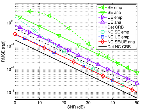
Figure 1: Analytical and empirical RMSEs versus SNR for a $4\times 4\times 4$ cubic uniform array ($R=3$), and $N=5$, $d=2$ correlated sources ($\rho=0.9$) at $\mu_{1}^{(1)}=0$, $\mu_{2}^{(1)}=0.1$, $\mu_{1}^{(2)}=0$, $\mu_{2}^{(2)}=0.1$, $\mu_{1}^{(3)}=0$, $\mu_{2}^{(3)}=0.1$ with rotation phases $\varphi_{1}=0$, $\varphi_{2}=\pi/2$.

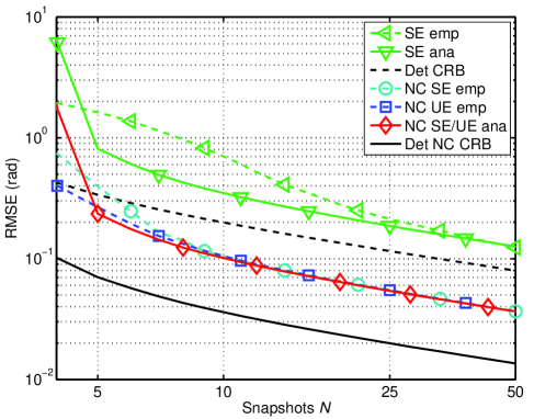
Figure 2: Analytical and empirical RMSEs versus the snapshots $N$ for the 20-element 2-D array ($R=2$) from Fig. 3 and SNR $=10$ dB, $d=3$ uncorrelated sources at $\mu_{1}^{(1)}=0.25$, $\mu_{2}^{(1)}=0.5$, $\mu_{3}^{(1)}=0.75$, $\mu_{1}^{(2)}=0.25$, $\mu_{2}^{(2)}=0.5$, $\mu_{3}^{(2)}=0.75$ with rotation phases $\varphi_{1}=0$, $\varphi_{2}=\pi/4$, $\varphi_{3}=\pi/2$.

\psfrag{Jxx}{\footnotesize{\color[rgb]{1,0,0} $\bm{{\tilde{J}}}_{1}^{(1)}$}}\psfrag{J12}{\footnotesize{\color[rgb]{0,1,0} $\bm{{\tilde{J}}}_{2}^{(1)}$}}\psfrag{J21}{\footnotesize{\color[rgb]{1,0,0} $\bm{{\tilde{J}}}_{1}^{(2)}$}}\psfrag{J22}{\footnotesize{\color[rgb]{0,1,0} $\bm{{\tilde{J}}}_{2}^{(2)}$}}\includegraphics[width=303.53267pt]{Figures/array_2d_shinv}

Figure 3: 2-D shift invariance for the depicted non-centro-symmetric $5\times 4$ sampling grid, left: subarrays for the first (horizontal) dimension, right: subarrays for the second (vertical) dimension.

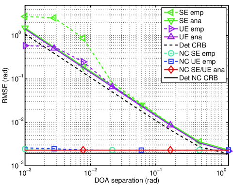
Figure 4: Analytical and empirical RMSEs versus the separation (“sep”) of $d=2$ uncorrelated sources at $\mu_{1}^{(1)}=-\textrm{sep}/2$, $\mu_{2}^{(1)}=0$, $\mu_{1}^{(2)}=\textrm{sep}/2$, $\mu_{2}^{(2)}=\textrm{sep}$ for a $5\times 6$ URA $(R=2)$, $N=5$, $\textrm{SNR}=30$ dB, with rotation phases $\varphi_{1}=0$, $\varphi_{2}=\pi/2$ .

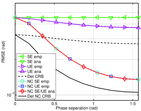
Figure 5: Analytical and empirical RMSEs versus the phase separation for a $5\times 6$ URA $(R=2)$, $N=5$, $\textrm{SNR}=30$ dB, $d=2$ uncorrelated sources at $\mu_{1}^{(1)}=1$, $\mu_{2}^{(1)}=0.8$, $\mu_{1}^{(2)}=1$, $\mu_{2}^{(2)}=0.8$.

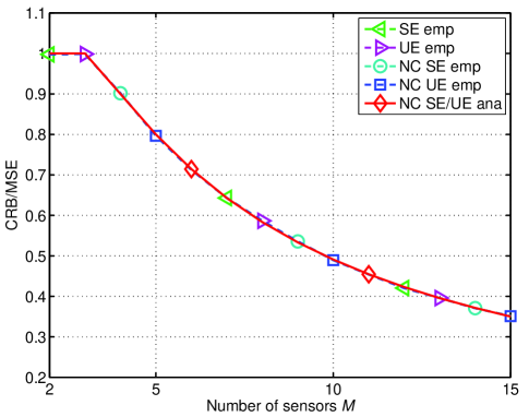
Figure 6: Asymptotic efficiency versus $M$ of a ULA $(R=1)$ for a single strictly non-circular source with an effective SNR of $46$ dB ($P_{\mathrm{s}}=0$ dB, $N=4$, $\sigma_{n}^{2}=10^{-4}$).

Fig. 1 illustrates the RMSE versus the SNR, where we consider a $4\times 4\times 4$ uniform cubic array with $N=5$ available observations of $d=2$ sources with the spatial frequencies $\mu_{1}^{(1)}=0$, $\mu_{2}^{(1)}=0.1$, $\mu_{1}^{(2)}=0$, $\mu_{2}^{(2)}=0.1$, $\mu_{1}^{(3)}=0$, and $\mu_{2}^{(3)}=0.1$, and a real-valued pair-wise correlation of $\rho=0.9$. The rotation phases contained in $\bm{\Psi}$ are given by $\varphi_{1}=0$ and $\varphi_{2}=\pi/2$. In Fig. 2, we depict the RMSE versus the number of snapshots $N$ for the non-centro-symmetric 2-D array with $M=20$ given in Fig. 3, where we also provide the subarrays in both dimensions. The SNR is fixed at $10$ dB and we have $d=3$ uncorrelated sources with the spatial frequencies $\mu_{1}^{(1)}=0.25$, $\mu_{2}^{(1)}=0.5$, $\mu_{3}^{(1)}=0.75$, $\mu_{1}^{(2)}=0.25$, $\mu_{2}^{(2)}=0.5$, and $\mu_{3}^{(2)}=0.75$. The rotation phases are given by $\varphi_{1}=0$, $\varphi_{2}=\pi/4$, and $\varphi_{3}=\pi/2$. Note that 2-D Unitary ESPRIT cannot be applied as the array is not centro-symmetric. It is apparent from Fig. 1 and Fig. 2 that in general, the NC schemes perform better than their non-NC counterparts. Specifically, $R$-D NC Unitary ESPRIT provides a lower estimation error than $R$-D NC Standard ESPRIT for low SNRs and a low sample size. Moreover, the analytical results agree well with the empirical estimation errors for high effective SNRs, i.e., when either the SNR or the number of samples becomes large. This also validates that the asymptotic performance of $R$-D NC Standard ESPRIT and $R$-D NC Unitary ESPRIT is identical as both coincide with the analytical curve. Note that the performance of the proposed algorithms can degrade if the signals’ non-circularity is not perfectly strict.

In Fig. 4, we show the RMSE as a function of the separation (“sep”) between $d=2$ uncorrelated sources located at $\mu_{1}^{(1)}=-\textrm{sep}/2$, $\mu_{2}^{(1)}=0$, $\mu_{1}^{(2)}=\textrm{sep}/2$, $\mu_{2}^{(2)}=\textrm{sep}$ with the rotation phases $\varphi_{1}=0$, $\varphi_{2}=\pi/2$. We employ a $5\times 6$ uniform rectangular array (URA), $N=5$ snapshots, and the SNR is fixed at $30$ dB. Fig. 5 demonstrates the RMSE as a function of the non-circularity phase separation $\Delta\varphi$ of the $d=2$ uncorrelated sources with the spatial frequencies $\mu_{1}^{(1)}=1$, $\mu_{2}^{(1)}=0.8$, $\mu_{1}^{(2)}=1$, and $\mu_{2}^{(2)}=0.8$. The remaining parameters are kept the same. Again, it can be seen from Fig. 4 and Fig. 5 that the analytical results match the empirical ones. But more importantly, the gain of the NC ESPRIT-type methods increases if the sources approach each other. Furthermore, as a substantial feature of strictly non-circular sources, it is observed that for two uncorrelated sources with a phase separation of $\Delta\varphi=\pi/2$, the sources entirely decouple as if each of them was present alone. In this case, the achievable gain from strictly non-circular sources is largest, which is verified by Fig. 5. This decoupling effect was also shown analytically for the Det NC CRB in [32] and recently for NC Standard ESPRIT in [41].

In the final simulation, we consider the single source case, which was used in Section VI to express the analytical MSE equations of $R$-D NC Standard ESPRIT and $R$-D NC Unitary ESPRIT only in terms of the physical parameters, i.e., the array size $M$ and the effective SNR. Fig. 6 shows the asymptotic efficiency (43) for the case $R=1$ versus the number of sensors $M$ of a ULA. The effective SNR is set to $46$ dB, where $P_{\mathrm{s}}=0$ dB, $N=4$, and $\sigma_{n}^{2}=10^{-4}$. This plot validates the fact that 1-D NC Standard ESPRIT and 1-D NC Unitary ESPRIT using LS become increasingly inefficient for $M>3$. It should be stressed that the same curves are obtained for 1-D Standard ESPRIT and 1-D Unitary ESPRIT. Hence, no gain is achieved from a single strictly non-circular source.

VIII Conclusion

In this paper, we have presented the $R$-D NC Standard ESPRIT and $R$-D NC Unitary ESPRIT parameter estimation algorithms specifically designed for strictly SO non-circular sources and shift-invariant arrays that are not necessarily centro-symmetric. We have also derived a first-order analytical performance analysis of both algorithms. Our results are based on a first-order expansion of the estimation error in terms of the explicit noise perturbation, which is required to be small compared to the signals but no assumptions about the noise statistics are needed. We have also derived MSE expressions that only depend on the finite SO moments of the noise and merely assume the noise to be zero-mean. All the resulting expressions are asymptotic in the effective SNR, i.e., they become accurate for either high SNRs or a large sample size. Furthermore, we have analytically proven that $R$-D NC Standard ESPRIT and $R$-D NC Unitary ESPRIT have the same asymptotic performance in the high effective SNR regime. However, $R$-D NC Unitary ESPRIT should be preferred due to its real-valued operations and its better performance at low effective SNRs. We have also computed the 1-D asymptotic efficiency for a single source and found that no gain from non-circular sources is achieved in this case. Simulations demonstrate that for more than one strictly non-circular source, the NC gain is largest for closely-spaced sources and a rotation phase separation of $\pi/2$.

Appendix A Proof of Theorem 1

We consider the 1-D case for simplicity and start by inserting $\bm{J}^{({\rm nc})}_{1}$ and $\bm{J}^{({\rm nc})}_{2}$ into (8), which yields

$$\begin{bmatrix}\bm{J}_{1}\bm{A}\\ \bm{\Pi}_{M^{({\rm sel})}}\bm{J}_{2}\bm{\Pi}_{M}\bm{\Pi}_{M}\bm{A}^{*}\bm{\Psi}^{*}\bm{\Psi}^{*}\end{bmatrix}\bm{\Phi} =\begin{bmatrix}\bm{J}_{2}\bm{A}\\ \bm{\Pi}_{M^{({\rm sel})}}\bm{J}_{1}\bm{\Pi}_{M}\bm{\Pi}_{M}\bm{A}^{*}\bm{\Psi}^{*}\bm{\Psi}^{*}\end{bmatrix}\!\!.$$

The first $M^{({\rm sel})}$ rows are given by $\bm{J}_{1}\bm{A}\bm{\Phi}=\bm{J}_{2}\bm{A}$, which was assumed for the theorem. The second $M^{({\rm sel})}$ rows can be simplified by multiplying from the left with $\bm{\Pi}_{M^{({\rm sel})}}$ and then using the fact that $\bm{\Pi}_{M}\bm{\Pi}_{M}=\bm{I}_{M}$. We obtain

$$\bm{J}_{2}\bm{A}^{*}\bm{\Psi}^{*}\bm{\Psi}^{*}\bm{\Phi}=\bm{J}_{1}\bm{A}^{*}\bm{\Psi}^{*}\bm{\Psi}^{*}.$$ (45)

As $\bm{\Psi}$ and $\bm{\Phi}$ are diagonal, they commute. Then, multiplying twice by $\bm{\Psi}$ from the right-hand side cancels $\bm{\Psi}$ as $\bm{\Psi}^{*}\bm{\Psi}=\bm{I}_{d}$ and we are left with

$$\bm{J}_{2}\bm{A}^{*}\bm{\Phi} =\bm{J}_{1}\bm{A}^{*}$$

$$\bm{J}_{2}\bm{A}^{*} =\bm{J}_{1}\bm{A}^{*}\bm{\Phi}^{*},$$ (46)

where in the last step we have multiplied with $\bm{\Phi}^{*}$ from the right-hand side and used the fact that $\bm{\Phi}^{*}\bm{\Phi}=\bm{I}_{d}$. Finally, conjugating (46) shows that this expression is equivalent to $\bm{J}_{1}\bm{A}\bm{\Phi}=\bm{J}_{2}\bm{A}$, which was again assumed for the theorem. This concludes the proof. ∎

Appendix B Proof of Equation (21)

The real-valued transformation is carried out using sparse left $\bm{\Pi}$-real matrices of even order according to (15). Expanding (20) yields

$$\varphi(\tilde{\bm{X}}^{({\rm nc})})=\bm{Q}^{\rm H}_{2M}\tilde{\bm{X}}^{({\rm nc})}\bm{Q}_{2N}$$

$$=\frac{1}{2}\cdot\begin{bmatrix}\bm{I}_{M}&\bm{\Pi}_{M}\\ -\mathrm{j}\bm{I}_{M}&\mathrm{j}\bm{\Pi}_{M}\end{bmatrix}\begin{bmatrix}\bm{X}^{({\rm nc})}&\bm{X}^{({\rm nc})}\bm{\Pi}_{N}\end{bmatrix}\begin{bmatrix}\bm{I}_{N}&\mathrm{j}\bm{I}_{N}\\ \bm{\Pi}_{N}&-\mathrm{j}\bm{\Pi}_{N}\end{bmatrix}$$

$$=\begin{bmatrix}\bm{I}_{M}&\bm{\Pi}_{M}\\ -\mathrm{j}\bm{I}_{M}&\mathrm{j}\bm{\Pi}_{M}\end{bmatrix}\begin{bmatrix}\bm{X}&\bm{0}_{M\times N}\\ \bm{\Pi}_{M}\bm{X}^{*}&\bm{0}_{M\times N}\end{bmatrix}$$

$$=\begin{bmatrix}\bm{X}+\bm{X}^{*}&\bm{0}_{M\times N}\\ -\mathrm{j}\bm{X}+\mathrm{j}\bm{X}^{*}&\bm{0}_{M\times N}\end{bmatrix}=2\cdot\begin{bmatrix}\mathop{{\rm Re}}\left\{\bm{X}\right\}&\bm{0}_{M\times N}\\ \mathop{{\rm Im}}\left\{\bm{X}\right\}&\bm{0}_{M\times N}\end{bmatrix},$$

where we have used the fact that $-\mathrm{j}x+\mathrm{j}x^{*}=2\cdot\mathop{{\rm Im}}\left\{x\right\}~{}\forall x\in\mathbb{C}$. This completes the proof. ∎

Appendix C Proof of Theorem 4

For simplicity, we only present the proof for the 1-D case, but the approach adopted here carries over to the $R$-D case straightforwardly. The estimated parameters after the real-valued transformation (NC Unitary ESPRIT) are extracted in a different manner as in the forward-backward-averaged complex-valued case (NC Standard ESPRIT with FBA), i.e. using the arctangent function. Hence, we develop a first-order perturbation expansion for the real-valued shift invariance equations and then show the equivalence of both cases. To this end, let $\tilde{\bm{X}}^{({\rm nc})}_{0}\in\mathbb{C}^{2M\times 2N}$ be the noise-free forward-backward averaged measurement matrix defined by decomposing (19) according to

$$\tilde{\bm{X}}^{({\rm nc})} =\begin{bmatrix}\bm{X}_{0}^{({\rm nc})}&\bm{X}_{0}^{({\rm nc})}\bm{\Pi}_{N}\end{bmatrix}+\begin{bmatrix}\bm{N}^{({\rm nc})}&\bm{N}^{({\rm nc})}\bm{\Pi}_{N}\end{bmatrix}$$

$$=\tilde{\bm{X}}^{({\rm nc})}_{0}+\tilde{\bm{N}}^{({\rm nc})}.$$ (47)

Its SVD can be expressed as

$$\tilde{\bm{X}}^{({\rm nc})}_{0} =\begin{bmatrix}\tilde{\bm{U}}^{({\rm nc})}_{\rm s}&\tilde{\bm{U}}^{({\rm nc})}_{\rm n}\end{bmatrix}\begin{bmatrix}\tilde{\bm{\Sigma}}^{({\rm nc})}_{\rm s}&\bm{0}\\ \bm{0}&\bm{0}\end{bmatrix}\begin{bmatrix}\tilde{\bm{V}}^{({\rm nc})}_{\rm s}&\tilde{\bm{V}}^{({\rm nc})}_{\rm n}\end{bmatrix}^{\rm H},$$

such that the complex-valued shift invariance equation for the forward-backward-averaged data has the form

$$\bm{J}^{({\rm nc})}_{1}\tilde{\bm{U}}^{({\rm nc})}_{\rm s}\bm{\Gamma}=\bm{J}^{({\rm nc})}_{2}\tilde{\bm{U}}^{({\rm nc})}_{\rm s},$$ (48)

where $\bm{\Gamma}=\bm{Q}^{({\rm fba})}\bm{\Lambda}\bm{Q}^{({\rm fba})^{-1}}$ and $\bm{\Lambda}=\mathop{{\rm diag}}\left\{\begin{bmatrix}\lambda_{1},\ldots,\lambda_{d}\end{bmatrix}\right\}$ with $\lambda_{i}={{\rm e}}^{\mathrm{j}\mu_{i}}$, $i=1,2,\ldots,d$. Performing the same steps as in Section V-A, the first-order approximation of the estimation error after the application of FBA is given by

$$\begin{aligned} \Delta\mu_{i}&=\mathop{{\rm Im}}\left\{\bm{p}^{({\rm fba})^{\rm T}}_{i}\left(\bm{J}_{1}^{({\rm nc})}\tilde{\bm{U}}^{({\rm nc})}_{\rm s}\right)^{+}\left[\bm{J}_{2}^{({\rm nc})}/\lambda_{i}\right.\right.\\ &\qquad~{}~{}\qquad\left.\left.-\bm{J}_{1}^{({\rm nc})}\right]\Delta\tilde{\bm{U}}^{({\rm nc})}_{\rm s}\bm{q}^{({\rm fba})}_{i}\right\}+\mathcal{O}\{\nu^{2}\},\end{aligned}$$ (49)

where we have simply replaced the corresponding quantities in (29) by their FBA versions. Next, we show that the estimation error expansion for the real-valued case is equivalent to (49).

The 1-D real-valued shift-invariance equation

$$\bm{K}^{({\rm nc})}_{1}\bm{E}^{({\rm nc})}_{\rm s}\bm{\Upsilon}=\bm{K}^{({\rm nc})}_{2}\bm{E}^{({\rm nc})}_{\rm s},$$ (50)

where $\bm{\Upsilon}=\bm{V}\bm{\Omega}\bm{V}^{-1}$ and $\bm{\Omega}=\mathop{{\rm diag}}\left\{\begin{bmatrix}\omega_{1},\ldots,\omega_{d}\end{bmatrix}\right\}$ with $\omega_{i}=\tan(\mu_{i}/2)$, $i=1,2,\ldots,d$, has the same algebraic form as its complex-valued counterpart in (48). Therefore, the same procedure from [8] can be applied to develop a first-order perturbation expansion. In fact, following the three steps discussed in [8], we find that the perturbation of $\omega_{i}$ in terms of $\bm{\Upsilon}$ and the perturbation of $\bm{\Upsilon}$ in terms of the signal subspace estimation error $\Delta\tilde{\bm{U}}^{({\rm nc})}_{\rm s}$ lead to the same result, where $\bm{J}^{({\rm nc})}_{1},\bm{J}^{({\rm nc})}_{2},\bm{U}^{({\rm nc})}_{\rm s}$, and $\bm{\Gamma}$ are consistently exchanged by $\bm{K}^{({\rm nc})}_{1},\bm{K}^{({\rm nc})}_{2},\bm{E}^{({\rm nc})}_{\rm s}$, and $\bm{\Upsilon}$, respectively. Thus, only the perturbation of $\mu_{i}$ in terms of $\omega_{i}=\tan(\mu_{i}/2)$ is to be derived. Therefore, we compute the Taylor series expansion of $\omega_{i}$, which is given by

$$\omega_{i}+\Delta\omega \approx\tan(\mu_{i}/2)+\Delta\mu\left(\frac{\tan^{2}(\mu_{i}/2)}{2}+\frac{1}{2}\right)$$

$$=\omega_{i}+\Delta\mu~{}\frac{\omega_{i}^{2}+1}{2}\quad\textrm{and hence}$$

$$\Delta\mu \approx\Delta\omega\frac{2}{\omega_{i}^{2}+1}.$$ (51)

Combining (51) with the corresponding real-valued expressions for the perturbations of $\omega_{i}$ and $\bm{\Upsilon}$, we obtain

$$\begin{aligned} \Delta\mu_{i}&=\bar{\bm{p}}_{i}^{\rm T}\left(\bm{K}^{({\rm nc})}_{1}\bm{E}^{({\rm nc})}_{\rm s}\right)^{+}\left(\bm{K}^{({\rm nc})}_{2}-\omega_{i}\bm{K}^{({\rm nc})}_{1}\right)\\ &\qquad\qquad\cdot\Delta\bm{E}^{({\rm nc})}_{\rm s}\bar{\bm{q}_{i}}\frac{2}{\omega_{i}^{2}+1},\end{aligned}$$ (52)

where $\bar{\bm{q}}_{i}$ is the $i$-th column of $\bm{V}$ and $\bar{\bm{p}}_{i}^{\rm T}$ is the $i$-th row of $\bm{V}^{-1}$. Moreover, the perturbation of the real-valued subspace $\bm{E}^{({\rm nc})}_{\rm s}$ is expanded in terms of the transformed noise contribution $\varphi(\tilde{\bm{N}}^{({\rm nc})})=\bm{Q}_{2M}^{\rm H}\tilde{\bm{N}}^{({\rm nc})}\bm{Q}_{2N}$ as

$$\Delta\bm{E}^{({\rm nc})}_{\rm s}=\bm{E}^{({\rm nc})}_{\rm n}\bm{E}^{({\rm nc})^{\rm H}}_{\rm n}\varphi(\tilde{\bm{N}}^{({\rm nc})})\bm{W}^{({\rm nc})}_{\rm s}\bm{\Sigma}^{(\varphi)^{-1}}_{\rm s},$$ (53)

where the required subspaces are obtained from the SVD of the transformed real-valued measurement matrix $\varphi(\tilde{\bm{X}}^{({\rm nc})}_{0})=\bm{Q}_{2M}^{\rm H}\tilde{\bm{X}}^{({\rm nc})}_{0}\bm{Q}_{2N}\in{}^{2M\times 2N}$ expressed as

$$\varphi(\tilde{\bm{X}}^{({\rm nc})}_{0}) =\begin{bmatrix}\bm{E}^{({\rm nc})}_{\rm s}&\!\!\bm{E}^{({\rm nc})}_{\rm n}\end{bmatrix}\begin{bmatrix}\bm{\Sigma}_{{\rm s}}^{(\varphi)}&\bm{0}\\ \bm{0}&\bm{0}\end{bmatrix}\begin{bmatrix}\bm{W}^{({\rm nc})}_{\rm s}&\!\!\bm{W}^{({\rm nc})}_{\rm n}\end{bmatrix}^{\rm H}.$$

To simplify (52), it is easy to see that due to the fact that the matrices $\bm{Q}_{p}$ are unitary, the subspaces of $\varphi(\tilde{\bm{X}}^{({\rm nc})}_{0})$ are also given by choosing

$$\bm{E}^{({\rm nc})}_{\rm s} =\bm{Q}_{2M}^{\rm H}\tilde{\bm{U}}^{({\rm nc})}_{\rm s},~{}\bm{E}^{({\rm nc})}_{\rm n}=\bm{Q}_{2M}^{\rm H}\tilde{\bm{U}}^{({\rm nc})}_{\rm n},~{}\bm{\Sigma}_{{\rm s}}^{(\varphi)}=\tilde{\bm{\Sigma}}^{({\rm nc})}_{\rm s}$$

$$\bm{W}^{({\rm nc})}_{\rm s} =\bm{Q}_{2N}^{\rm H}\tilde{\bm{V}}^{({\rm nc})}_{\rm s},~{}\bm{W}^{({\rm nc})}_{\rm n}=\bm{Q}_{2N}^{\rm H}\tilde{\bm{V}}^{({\rm nc})}_{\rm n}.$$ (54)

Moreover, the transformed selection matrices $\bm{K}^{({\rm nc})}_{1}$ and $\bm{{K}}^{({\rm nc})}_{2}$ defined in (23) and (24) can be reformulated as

$$\bm{{K}}^{({\rm nc})}_{1} =~{}\bm{Q}^{\rm H}_{2M^{({\rm sel})}}\big{(}\bm{J}^{({\rm nc})}_{1}+\bm{J}^{({\rm nc})}_{2}\big{)}~{}\bm{Q}_{2M}$$ (55)

$$\bm{K}^{({\rm nc})}_{2} =\mathrm{j}\cdot\bm{Q}^{\rm H}_{2M^{({\rm sel})}}\big{(}\bm{J}^{({\rm nc})}_{1}-\bm{J}^{({\rm nc})}_{2}\big{)}~{}\bm{Q}_{2M},$$ (56)

which follows from expanding the real part and the imaginary part according to $2\cdot\mathop{{\rm Re}}\left\{x\right\}=x+x^{*}$ and $2\cdot\mathop{{\rm Im}}\left\{x\right\}=-\mathrm{j}x+\mathrm{j}x^{*}$. The conjugated term $\bm{Q}_{2M^{({\rm sel})}}^{\rm T}\bm{J}^{({\rm nc})}_{2}\bm{Q}_{2M}^{*}$ can be simplified to $\bm{Q}_{2M^{({\rm sel})}}^{\rm H}\bm{J}^{({\rm nc})}_{1}\bm{Q}_{2M}$ using the fact that $\bm{J}^{({\rm nc})}_{1}=\bm{\Pi}_{2M^{({\rm sel})}}\bm{J}^{({\rm nc})}_{2}\bm{\Pi}_{2M}$ holds since the virtual array is always centro-symmetric as shown in Theorem 2 and the fact that $\bm{Q}_{p}$ is left-$\bm{\Pi}$-real.

Inserting (53) into (52) and applying the identities (54)-(56), we have

$$\Delta\mu_{i} =\bar{\bm{p}}_{i}^{\rm T}\Big{(}\big{(}\bm{J}^{({\rm nc})}_{1}+\bm{J}^{({\rm nc})}_{2}\big{)}\tilde{\bm{U}}^{({\rm nc})}_{\rm s}\Big{)}^{+}\Big{(}\mathrm{j}\cdot\big{(}\bm{J}^{({\rm nc})}_{1}-\bm{J}^{({\rm nc})}_{2}\big{)}$$

$$~{}~{}~{}-\omega_{i}\big{(}\bm{J}^{({\rm nc})}_{1}+\bm{J}^{({\rm nc})}_{2}\big{)}\Big{)}\Delta\tilde{\bm{U}}^{({\rm nc})}_{\rm s}\bar{\bm{q}}_{i}\frac{2}{\omega_{i}^{2}+1},$$ (57)

where $\Delta\tilde{\bm{U}}^{({\rm nc})}_{\rm s}=\tilde{\bm{U}}^{({\rm nc})}_{\rm n}\tilde{\bm{{U}}_{\rm n}}^{({\rm nc})^{\rm H}}\tilde{\bm{N}}^{({\rm nc})}\tilde{\bm{V}}^{({\rm nc})}_{s}\tilde{\bm{\Sigma}}^{({\rm nc})^{-1}}_{\rm s}$.

In order to further simplify (57), we require the following two lemmas:

Lemma 1.

The following identities are satisfied

$$\big{(}\bm{J}^{({\rm nc})}_{1}+\bm{J}^{({\rm nc})}_{2}\big{)}\tilde{\bm{U}}^{({\rm nc})}_{\rm s} =\bm{J}^{({\rm nc})}_{1}\tilde{\bm{U}}^{({\rm nc})}_{\rm s}\breve{\bm{\Gamma}}$$ (58)

$$\big{(}\bm{J}^{({\rm nc})}_{1}-\bm{J}^{({\rm nc})}_{2}\big{)}\tilde{\bm{U}}^{({\rm nc})}_{\rm s} =\bm{J}^{({\rm nc})}_{2}\tilde{\bm{U}}^{({\rm nc})}_{\rm s}\mathring{\bm{\Gamma}},$$ (59)

where $\breve{\bm{\Gamma}}=\bm{I}_{d}+\bm{\Gamma}=\bm{Q}^{({\rm fba})}\left(\bm{I}_{d}+\bm{\Lambda}\right)\bm{Q}^{({\rm fba})^{-1}}$ and $\mathring{\bm{\Gamma}}=-\bm{I}_{d}+\bm{\Gamma}^{-1}=\bm{Q}^{({\rm fba})}\left(-\bm{I}_{d}+\bm{\Lambda}^{-1}\right)\bm{Q}^{({\rm fba})^{-1}}$.

Proof:

These identities follow straightforwardly from $\bm{J}^{({\rm nc})}_{1}\tilde{\bm{U}}^{({\rm nc})}_{\rm s}\bm{\Gamma}=\bm{J}^{({\rm nc})}_{2}\tilde{\bm{U}}^{({\rm nc})}_{\rm s}$ by adding $\bm{J}^{({\rm nc})}_{1}\tilde{\bm{U}}^{({\rm nc})}_{\rm s}$ to both sides of the equation for the first identity, and subtracting $\bm{J}^{({\rm nc})}_{1}\tilde{\bm{U}}^{({\rm nc})}_{\rm s}$ and substituting $\bm{J}^{({\rm nc})}_{1}\tilde{\bm{U}}^{({\rm nc})}_{\rm s}$ by $\bm{J}^{({\rm nc})}_{2}\tilde{\bm{U}}^{({\rm nc})}_{\rm s}\bm{\Gamma}^{-1}$ for the second identity. ∎

Lemma 2.

In the noiseless case, the solution $\bm{\Gamma}$ to (48) and the solution $\bm{\Upsilon}$ to (50) have the same eigenvectors, i.e., $\bm{Q}^{({\rm fba})}=\bm{V}$. Moreover, their eigenvalues are related as $\omega_{i}=\mathrm{j}\cdot\frac{1-\lambda_{i}}{1+\lambda_{i}}$.

Proof:

Starting from $\bm{\Upsilon}=\big{(}\bm{K}^{({\rm nc})}_{1}\bm{E}^{({\rm nc})}_{\rm s}\big{)}^{+}\bm{K}^{({\rm nc})}_{2}\bm{E}^{({\rm nc})}_{\rm s}$ and replacing $\bm{E}^{({\rm nc})}_{\rm s}$ with (54) and $\bm{K}^{({\rm nc})}_{n}$ with (55) and (56), we get

$$\bm{\Upsilon} =\left(\big{(}\bm{J}^{({\rm nc})}_{1}+\bm{J}^{({\rm nc})}_{2}\big{)}\tilde{\bm{U}}^{({\rm nc})}_{\rm s}\right)^{+}\mathrm{j}\cdot\big{(}\bm{J}^{({\rm nc})}_{1}-\bm{J}^{({\rm nc})}_{2}\big{)}\tilde{\bm{U}}^{({\rm nc})}_{\rm s}$$

$$=\mathrm{j}\cdot\breve{\bm{\Gamma}}^{-1}\bm{\Gamma}\mathring{\bm{\Gamma}}=\mathrm{j}\cdot\bm{Q}^{({\rm fba})}\left(\bm{I}_{d}+\bm{\Lambda}\right)^{-1}\left(\bm{I}_{d}-\bm{\Lambda}\right)\bm{Q}^{({\rm fba})^{-1}}$$

$$=\bm{Q}^{({\rm fba})}\bm{\Omega}\bm{Q}^{({\rm fba})^{-1}},$$ (60)

where $\bm{\Omega}=\mathop{{\rm diag}}\left\{\mathrm{j}\cdot\big{[}\frac{1-\lambda_{i}}{1+\lambda_{i}}\big{]}\right\}_{i=1}^{d}$ and we have used Lemma 1 in the first step. ∎

Next, we consider the term $\big{(}\mathrm{j}\cdot\big{(}\bm{J}^{({\rm nc})}_{1}-\bm{J}^{({\rm nc})}_{2}\big{)}-\omega_{i}\big{(}\bm{J}^{({\rm nc})}_{1}+\bm{J}^{({\rm nc})}_{2}\big{)}\big{)}$ in (57) and apply the relation $\omega_{i}=\mathrm{j}\cdot\frac{1-\lambda_{i}}{1+\lambda_{i}}$ from Lemma 2. We can then rewrite this term as $\mathrm{j}\cdot\big{(}\bm{J}^{({\rm nc})}_{1}\lambda_{i}-\bm{J}^{({\rm nc})}_{2}\big{)}\frac{2}{1+\lambda_{i}}$. Moreover, the term $\frac{2}{\omega_{i}^{2}+1}$ in (57) can be expressed in terms of $\lambda_{i}$ as $\frac{2}{\omega_{i}^{2}+1}=\frac{(\lambda_{i}+1)^{2}}{2\lambda_{i}}$. Inserting these relations into (57), replacing $\big{(}\bm{J}^{({\rm nc})}_{1}+\bm{J}^{({\rm nc})}_{2}\big{)}\tilde{\bm{U}}^{({\rm nc})}_{\rm s}$ via (58), and substituting $\bar{\bm{p}}_{i}=\bm{p}^{({\rm fba})}_{i}$ and $\bar{\bm{q}}_{i}=\bm{q}^{({\rm fba})}_{i}$ using Lemma 2, yields

$$\Delta\mu_{i} =\mathrm{j}\cdot\bm{p}^{({\rm fba})^{\rm T}}_{i}\breve{\bm{\Gamma}}^{-1}\left(\bm{J}^{({\rm nc})}_{1}\tilde{\bm{U}}^{({\rm nc})}_{\rm s}\right)^{+}\left(\bm{J}^{({\rm nc})}_{1}\lambda_{i}-\bm{J}^{({\rm nc})}_{2}\right)$$

$$\qquad\cdot\Delta\tilde{\bm{U}}^{({\rm nc})}_{\rm s}\bm{q}^{({\rm fba})}_{i}\frac{2}{1+\lambda_{i}}\cdot\frac{(\lambda_{i}+1)^{2}}{2\lambda_{i}}$$

$$=-\mathrm{j}\cdot\bm{p}^{({\rm fba})^{\rm T}}_{i}\left(\bm{J}^{({\rm nc})}_{1}\tilde{\bm{U}}^{({\rm nc})}_{\rm s}\right)^{+}\left(\bm{J}^{({\rm nc})}_{2}/\lambda_{i}-\bm{J}^{({\rm nc})}_{1}\right)$$

$$\qquad\cdot\Delta\tilde{\bm{U}}^{({\rm nc})}_{\rm s}\bm{q}^{({\rm fba})}_{i},$$ (61)

where we used $\bm{p}^{({\rm fba})^{\rm T}}_{i}\breve{\bm{\Gamma}}^{-1}=\bm{p}^{({\rm fba})^{\rm T}}_{i}(1+\lambda_{i})^{-1}$ from Lemma 1 in the first equation.

As a final step, we notice that (61) must be real-valued as we have started from the purely real-valued expansion (52) and only used equivalence transforms to arrive at (61). However, if $-\mathrm{j}z\in\real$ for $z\in\mathbb{C}$ this implies that $\mathop{{\rm Re}}\left\{z\right\}=0$ and hence $-\mathrm{j}z=\mathop{{\rm Im}}\left\{z\right\}$. Consequently, (61) can also be written as (49) and is therefore equivalent to the first-order expansion for $R$-D NC Standard ESPRIT with FBA. This concludes the proof of the theorem. ∎

Appendix D Proof of Theorem 5

We start the proof by simplifying the MSE expression for $R$-D NC Standard ESPRIT in (31). In the single source case the noise-free NC measurement matrix can be written as

$$\bm{X}_{0}^{({\rm nc})}=\bm{a}^{({\rm nc})}(\bm{\mu})\bm{s}^{\rm T},$$ (62)

where $\bm{a}^{({\rm nc})}(\bm{\mu})=[\bm{a}^{\rm T}(\bm{\mu}),\tilde{\Psi}\bm{\Pi}_{M}\bm{a}^{\rm H}(\bm{\mu})]^{\rm T}\in\mathbb{C}^{2M\times 1}$ is the augmented array steering vector and $\bm{a}(\bm{\mu})=\bm{a}^{(1)}(\mu^{(1)})\otimes\cdots\otimes\bm{a}^{(R)}(\mu^{(R)})~{}\in\mathbb{C}^{M\times 1}$. Moreover, $\tilde{\Psi}=\Psi^{*}\Psi^{*}={{\rm e}}^{-\mathrm{j}2\varphi}$, $\bm{s}\in\mathbb{C}^{N\times 1}$ contains the source symbols, and $\hat{P}_{\rm s}=\left\|\bm{s}\right\|_{2}^{2}/N$ is the empirical source power. In what follows, we drop the dependence of $\bm{a}^{({\rm nc})}$ on $\bm{\mu}$ for notational convenience. If we assume a ULA of isotropic elements in each of the $R$ modes, we have $\bm{a}^{({r})}=[1,{{\rm e}}^{\mathrm{j}\mu^{({r})}},\ldots,{{\rm e}}^{\mathrm{j}(M_{r}-1)\mu^{({r})}}]^{\rm T}$ and $\left\|\bm{a}^{({\rm nc})}\right\|_{2}^{2}=2M$. The selection matrices $\tilde{\bm{J}}^{({\rm nc})(r)}_{1}$ and $\tilde{\bm{J}}^{({\rm nc})(r)}_{2}$ are then chosen according to (9) with $\bm{J}_{1}^{({r})}=[\bm{I}_{M_{r}-1},\bm{0}_{(M_{r}-1)\times 1}]$ and $\bm{J}_{2}^{({r})}=[\bm{0}_{(M_{r}-1)\times 1},\bm{I}_{M_{r}-1}]$ for maximum overlap, i.e., $M_{r}^{({\rm sel})}=M_{r}-1$. Note that (62) is a rank-one matrix and we can directly determine the subspaces from the SVD as

$$\bm{U}_{\rm s}^{({\rm nc})} =\bm{u}_{\rm s}^{({\rm nc})}=\frac{\bm{a}^{({\rm nc})}}{\left\|\bm{a}^{({\rm nc})}\right\|_{2}}=\frac{\bm{a}^{({\rm nc})}}{\sqrt{2M}}$$

$$\bm{\Sigma}_{\rm s}^{({\rm nc})} =\sigma_{\rm s}^{({\rm nc})}=\sqrt{2MN\hat{P}_{\rm s}}$$

$$\bm{V}_{\rm s}^{({\rm nc})} =\bm{v}_{\rm s}^{({\rm nc})}=\frac{\bm{s}^{*}}{\left\|\bm{s}\right\|_{2}}=\frac{\bm{s}^{*}}{\sqrt{N\hat{P}_{\rm s}}}.$$

For the MSE expression in (31), we also require $\bm{P}^{\perp}_{\bm{a}^{({\rm nc})}}=\bm{U}_{\rm n}^{({\rm nc})}\bm{U}_{\rm n}^{({\rm nc})^{\rm H}}=\bm{I}_{2M}-\frac{1}{2M}\bm{a}^{({\rm nc})}\bm{a}^{({\rm nc})^{\rm H}}$, which is the projection matrix onto the noise subspace. Moreover, we have $\bm{\Gamma}^{({r})}={{\rm e}}^{\mathrm{j}\mu^{({r})}}$ and hence, the eigenvectors are $\bm{p}_{i}^{({r})}=\bm{q}_{i}^{({r})}=1$. The SO moments $\bm{R}_{\mathrm{nn}}^{({\rm nc})}$ and $\bm{C}_{\mathrm{nn}}^{({\rm nc})}$ of the noise are given by (39).

Inserting these expressions into (31), we get

$$\begin{aligned} &\quad\mathop{{\rm\mathbb{E}}}\left\{(\Delta\mu^{({r})})^{2}\right\}=\frac{\sigma_{\rm n}^{2}}{2}\left(\left\|\bm{r}^{({\rm nc})(r)^{\rm T}}\bm{W}^{({\rm nc})}\right\|_{2}^{2}\right.\\ &\left.-\mathop{{\rm Re}}\left\{\bm{r}^{({\rm nc})(r)^{\rm T}}\bm{W}^{({\rm nc})}(\bm{I}_{N}\otimes\bm{\Pi}_{2M})\left(\bm{r}^{({\rm nc})(r)^{\rm T}}\bm{W}^{({\rm nc})}\right)^{\rm T}\right\}\right)\end{aligned}$$ (63)

with

$$\bm{r}^{({\rm nc})(r)} =\left[\left(\tilde{\bm{J}}^{({\rm nc})(r)}_{1}\frac{\bm{a}^{({\rm nc})}}{\sqrt{2M}}\right)^{+}\!\!\left(\tilde{\bm{J}}^{({\rm nc})(r)}_{2}/{{\rm e}}^{\mathrm{j}\mu^{({r})}}-\tilde{\bm{J}}^{({\rm nc})(r)}_{1}\right)\right]^{\rm T},$$

$$\bm{W}^{({\rm nc})} =\left(\frac{1}{\sqrt{2MN\hat{P}_{\rm s}}}\cdot\frac{\bm{s}^{\rm H}}{\sqrt{N\hat{P}_{\rm s}}}\right)\otimes\bm{P}^{\perp}_{\bm{a}^{({\rm nc})}}~{}\in\mathbb{C}^{2M\times 2MN}.$$

Note that the term $\bm{r}^{({\rm nc})(r)^{\rm T}}\bm{W}^{({\rm nc})}$ can also be written as $\bm{r}^{({\rm nc})(r)^{\rm T}}\bm{W}^{({\rm nc})}=\tilde{\bm{s}}^{\rm T}\otimes\tilde{\bm{a}}^{({r})^{\rm T}}$, where

$$\tilde{\bm{s}}^{\rm T} =\frac{1}{\sqrt{2MN\hat{P}_{\rm s}}}\cdot\frac{\bm{s}^{\rm H}}{\sqrt{N\hat{P}_{\rm s}}},$$

$$\tilde{\bm{a}}^{({r})^{\rm T}} =\left(\tilde{\bm{J}}^{({\rm nc})(r)}_{1}\frac{\bm{a}^{({\rm nc})}}{\sqrt{2M}}\right)^{+}\!\!\!\left(\tilde{\bm{J}}^{({\rm nc})(r)}_{2}/{{\rm e}}^{\mathrm{j}\mu^{({r})}}-\tilde{\bm{J}}^{({\rm nc})(r)}_{1}\right)\bm{P}^{\perp}_{\bm{a}^{({\rm nc})}}.$$

Thus, after straightforward calculations, the MSE in (63) is given by

$$\begin{aligned} \mathop{{\rm\mathbb{E}}}\left\{(\Delta\mu^{({r})})^{2}\right\}&=\frac{\sigma_{\rm n}^{2}}{2}\left(\left\|\tilde{\bm{s}}^{\rm T}\right\|_{2}^{2}\cdot\left\|\tilde{\bm{a}}^{({r})^{\rm T}}\right\|_{2}^{2}\right.\\ &\qquad\bigg{.}-\mathop{{\rm Re}}\left\{\tilde{\bm{s}}^{\rm T}\tilde{\bm{s}}\cdot\tilde{\bm{a}}^{({r})^{\rm T}}\bm{\Pi}_{2M}\tilde{\bm{a}}^{({r})}\right\}\bigg{)}.\end{aligned}$$ (64)

The first term $\left\|\tilde{\bm{s}}^{\rm T}\right\|_{2}^{2}$ of (64) can be conveniently expressed as $\left\|\tilde{\bm{s}}^{\rm T}\right\|_{2}^{2}=\frac{1}{2MN\hat{P}_{\rm s}}$. For the second term $\big{\|}\tilde{\bm{a}}^{({r})^{\rm T}}\big{\|}_{2}^{2}$ of (64), we simplify $\tilde{\bm{a}}^{({r})^{\rm T}}$ and expand the pseudo-inverse of $\tilde{\bm{J}}^{({\rm nc})(r)}_{1}\bm{a}^{({\rm nc})(r)}$ using the relation $\bm{x}^{+}=\bm{x}^{\rm H}/\left\|\bm{x}\right\|_{2}^{2}$. As $\tilde{\bm{J}}^{({\rm nc})(r)}_{1}$ selects $2(M_{r}-1)$ out of $2M_{r}$ elements in the $r$-th mode, we have $\big{\|}\tilde{\bm{J}}^{({\rm nc})(r)}_{1}\bm{a}^{({\rm nc})(r)}\big{\|}_{2}^{2}=\frac{M}{M_{r}}\cdot 2(M_{r}-1)$. Then, taking the shift invariance equation $\tilde{\bm{J}}^{({\rm nc})(r)}_{2}\bm{a}^{({\rm nc})}/{{\rm e}}^{\mathrm{j}\mu^{({r})}}-\tilde{\bm{J}}^{({\rm nc})(r)}_{1}\bm{a}^{({\rm nc})}=\bm{0}$ in the $r$-th mode into account, we obtain

$$\tilde{\bm{a}}^{({r})^{\rm T}} =\frac{\sqrt{2M}M_{r}}{2M(M_{r}-1)}\left(\bm{a}^{({\rm nc})^{\rm H}}\tilde{\bm{J}}^{{({\rm nc})(r)}^{\rm H}}_{1}\tilde{\bm{J}}^{({\rm nc})(r)}_{2}/{{\rm e}}^{\mathrm{j}\mu^{({r})}}\right.$$

$$\qquad\left.-\bm{a}^{({\rm nc})^{\rm H}}\tilde{\bm{J}}^{{({\rm nc})(r)}^{\rm H}}_{1}\tilde{\bm{J}}^{({\rm nc})(r)}_{1}\right).$$ (65)

As a ULA is centro-symmetric, i.e., (10) holds, we can write $\bm{a}^{({\rm nc})}=[1,\tilde{\Psi}]^{\rm T}\otimes\bm{a}$. Note that the phase term depending on the phase center in (10) cancels throughout the derivation and thus has been neglected. Since the vector $\bm{a}$ and the matrices $\tilde{\bm{J}}^{({\rm nc})(r)}_{k},~{}k=1,2$, can be written as $\bm{a}=\bm{a}^{(1)}\otimes\cdots\otimes\bm{a}^{(R)}$ and $\tilde{\bm{J}}^{({\rm nc})(r)}_{k}=\bm{I}_{2}\otimes\bm{I}_{\prod_{l=1}^{r-1}M_{l}}\otimes\bm{J}^{({r})}_{k}\otimes\bm{I}_{\prod_{l=r+1}^{R}M_{l}}$, all the unaffected modes can be factored out of (65), yielding

$$\tilde{\bm{a}}^{({r})^{\rm T}}=\frac{\sqrt{2M}M_{r}}{2M(M_{r}-1)}\cdot\begin{bmatrix}1\\ \tilde{\Psi}\end{bmatrix}\otimes\left(\bm{a}^{(1)}\otimes\cdots\otimes\bm{a}^{(r-1)}\right)^{\rm H}$$

$$\otimes\left(\tilde{\bm{a}}^{({r})^{\rm T}}_{1}-\tilde{\bm{a}}^{({r})^{\rm T}}_{2}\right)\otimes\left(\bm{a}^{(r+1)}\otimes\cdots\otimes\bm{a}^{(R)}\right)^{\rm H},$$ (66)

where

$$\tilde{\bm{a}}^{({r})^{\rm T}}_{1} =\bm{a}^{({r})^{\rm H}}\bm{J}^{({r})^{\rm H}}_{1}\bm{J}^{({r})}_{2}/{{\rm e}}^{\mathrm{j}\mu^{({r})}}~{}~{}\textrm{and}$$

$$\tilde{\bm{a}}^{({r})^{\rm T}}_{2} =\bm{a}^{({r})^{\rm H}}\bm{J}^{({r})^{\rm H}}_{1}\bm{J}^{({r})}_{1}.$$

Similarly to [15], it is easy to verify that

$$\tilde{\bm{a}}^{({r})^{\rm T}}_{1} {=}\left[0,{{\rm e}}^{-\mathrm{j}\mu^{({r})}},\ldots,{{\rm e}}^{-\mathrm{j}(M_{r}-2)\mu^{({r})}},{{\rm e}}^{-\mathrm{j}(M_{r}-1)\mu^{({r})}}\right]$$

$$\tilde{\bm{a}}^{({r})^{\rm T}}_{2} {=}\left[1,{{\rm e}}^{-\mathrm{j}\mu^{({r})}},\ldots,{{\rm e}}^{-\mathrm{j}(M_{r}-2)\mu^{({r})}},0\right].$$

Consequently, we obtain

$$\left\|\tilde{\bm{a}}^{({r})^{\rm T}}\right\|_{2}^{2} =\frac{M_{r}^{2}}{2M(M_{r}-1)^{2}}\cdot 2\cdot\prod_{n=1}^{r-1}\left\|\bm{a}^{(n)}\right\|_{2}^{2}\cdot 2\cdot\!\!\prod_{n=r+1}^{R}\left\|\bm{a}^{(n)}\right\|_{2}^{2}$$

$$=\frac{2M_{r}^{2}}{M(M_{r}-1)^{2}}\cdot\frac{M}{M_{r}}=\frac{2M_{r}}{(M_{r}-1)^{2}}.$$ (67)

The third term $\tilde{\bm{s}}^{\rm T}\tilde{\bm{s}}$ of (64) can be simplified as $\tilde{\bm{s}}^{\rm T}\tilde{\bm{s}}=\frac{\tilde{\Psi}}{2MN\hat{P}_{\rm s}}$, where we have used the equality $\bm{s}=\Psi\bm{s}_{0}$ and the fact that $\bm{s}_{0}^{\rm T}\bm{s}_{0}=N\hat{P}_{\rm s}$. Moreover, using (66), the last term of (64) can be reduced to $\tilde{\bm{a}}^{({r})^{\rm T}}\bm{\Pi}_{2M}\tilde{\bm{a}}^{({r})}=-\frac{2M_{r}\tilde{\Psi}^{*}}{(M_{r}-1)^{2}}$. Inserting these results into (64), we finally obtain for the MSE of $R$-D NC Standard ESPRIT

$$\mathop{{\rm\mathbb{E}}}\left\{(\Delta\mu^{({r})})^{2}\right\}=\frac{\sigma_{\rm n}^{2}}{N\hat{P}_{\rm s}}\cdot\frac{M_{r}}{M(M_{r}-1)^{2}},$$ (68)

which is the desired result. ∎

Appendix E Proof of Theorem 6

We first state the expression for the deterministic NC CRB $\bm{C}^{({\rm nc})}$ derived in [32], which is given in the $R$-D case by

$$\bm{C}^{({\rm nc})}=\frac{\sigma^{2}_{\mathrm{n}}}{2N}\cdot\mathop{{\rm Re}}\left\{\bm{J}\right\}^{-1}$$ (69)

with

$$\bm{J}=\left(\bm{G}_{2}-\bm{G}_{1}\bm{G}_{0}^{-1}\bm{G}_{1}^{\rm T}\right)\odot\hat{\bm{R}}^{(R)}$$

$$+\!\left[\left(\bm{G}_{1}\bm{G}_{0}^{-1}\bm{H}_{0}\right)\odot\hat{\bm{R}}^{(R)}\right]\!\left[\left(\bm{G}_{0}-\bm{H}_{0}^{\rm T}\bm{G}_{0}^{-1}\bm{H}_{0}\right)\odot\hat{\bm{R}}^{(R)}\right]^{-1}$$

$$\cdot\left[\left(\bm{H}_{1}^{\rm T}-\bm{H}_{0}^{\rm T}\bm{G}_{0}^{-1}\bm{G}_{1}^{\rm T}\right)\odot\hat{\bm{R}}^{(R)}\right]+\left[\bm{H}_{1}\odot\hat{\bm{R}}^{(R)}\right]$$

$$\cdot\left[\bm{G}_{0}\odot\hat{\bm{R}}^{(R)}\right]^{-1}\!\!\!\cdot\left[\left(\bm{H}_{0}^{\rm T}\bm{G}_{0}^{-1}\bm{G}_{1}^{\rm T}\right)\odot\hat{\bm{R}}^{(R)}\right]+\left[\bm{H}_{1}\odot\hat{\bm{R}}^{(R)}\right]$$

$$\cdot\left[\bm{G}_{0}\odot\hat{\bm{R}}^{(R)}\right]^{-1}\cdot\left[\left(\bm{H}_{0}^{\rm T}\bm{G}_{0}^{-1}\bm{H}_{0}\right)\odot\hat{\bm{R}}^{(R)}\right]$$

$$\cdot\left[\left(\bm{G}_{0}-\bm{H}_{0}^{\rm T}\bm{G}_{0}^{-1}\bm{H}_{0}\right)\odot\hat{\bm{R}}^{(R)}\right]^{-1}\!\!\!{\cdot}\left[\left(\bm{H}_{0}^{\rm T}\bm{G}_{0}^{-1}\bm{G}_{1}^{\rm T}\right)\odot\hat{\bm{R}}^{(R)}\right]$$

$$-\left[\bm{H}_{1}\odot\hat{\bm{R}}^{(R)}\right]\cdot\left[\left(\bm{G}_{0}-\bm{H}_{0}^{\rm T}\bm{G}_{0}^{-1}\bm{H}_{0}\right)\odot\hat{\bm{R}}^{(R)}\right]^{-1}$$

$$\cdot\left[\bm{H}_{1}^{\rm T}\odot\hat{\bm{R}}^{(R)}\right],$$ (70)

where $\hat{\bm{R}}^{(R)}=\bm{1}_{R}\otimes\hat{\bm{R}}_{S_{0}}$ and $\hat{\bm{R}}_{S_{0}}=\bm{S}_{0}\bm{S}_{0}^{\rm T}/N$. The matrices $\bm{G}_{n},~{}\bm{H}_{n},~{}n=0,1,2$, are defined as

$$\bm{G}_{0} =\mathop{{\rm Re}}\left\{\bm{\Psi}^{*}\bm{A}^{\rm H}\bm{A}\bm{\Psi}\right\},~{}\bm{H}_{0}=\mathop{{\rm Im}}\left\{\bm{\Psi}^{*}\bm{A}^{\rm H}\bm{A}\bm{\Psi}\right\}$$ (71)

$$\bm{G}_{1} =\mathop{{\rm Re}}\left\{(\bm{I}_{R}\otimes\bm{\Psi}^{*})\bm{D}^{\rm H}\bm{A}\bm{\Psi}\right\},$$ (72)

$$\bm{H}_{1} =\mathop{{\rm Im}}\left\{(\bm{I}_{R}\otimes\bm{\Psi}^{*})\bm{D}^{\rm H}\bm{A}\bm{\Psi}\right\},$$ (73)

$$\bm{G}_{2} =\mathop{{\rm Re}}\left\{(\bm{I}_{R}\otimes\bm{\Psi}^{*})\bm{D}^{\rm H}\bm{D}(\bm{I}_{R}\otimes\bm{\Psi})\right\},$$ (74)

where $\bm{D}=[\bm{D}^{(1)},\ldots,\bm{D}^{(R)}]\in\mathbb{C}^{M\times dR}$ with $\bm{D}^{(r)}=[\bm{d}^{({r})}_{1},\ldots,\bm{d}^{({r})}_{d}]\in\mathbb{C}^{M\times d},~{}r=1,\ldots,R$. The vectors $\bm{d}^{({r})}_{i},~{}i=1,\ldots,d$, contain the partial derivatives $\partial\bm{a}(\bm{\mu}_{i})/\partial\mu^{({r})}_{i}$. In the special case $d=1$, the array steering matrix $\bm{A}$ reduces to $\bm{a}(\bm{\mu})$, $\bm{D}=[\bm{d}^{(1)},\ldots,\bm{d}^{(R)}]\in\mathbb{C}^{M\times R}$, $\bm{\Psi}={{\rm e}}^{\mathrm{j}\varphi}$, and $\bm{\hat{}}{R}_{S_{0}}=\bm{s}_{0}^{\rm T}\bm{s}_{0}/N=\hat{P}_{\mathrm{s}}$, where $\bm{s}_{0}\in{}^{N\times 1}$. Dropping the dependence of $\bm{a}$ on $\bm{\mu}$ and using the fact that $\bm{a}=\bm{a}^{(1)}\otimes\cdots\otimes\bm{a}^{(R)}$, we obtain

$$\bm{d}^{({r})}=\bm{a}^{(1)}\otimes\cdots\otimes\bm{a}^{(r-1)}\otimes\tilde{\bm{d}}^{({r})}\otimes\bm{a}^{(r+1)}\otimes\cdots\otimes\bm{a}^{(R)}.$$

For a ULA in each of the $R$ modes, we have $\bm{a}^{({r})}=[1,{{\rm e}}^{\mathrm{j}\mu^{({r})}},\ldots,{{\rm e}}^{\mathrm{j}(M_{r}-1)\mu^{({r})}}]^{\rm T}$ and $\tilde{\bm{d}}^{({r})}=\partial\bm{a}^{({r})}/\partial\mu^{({r})}=\mathrm{j}\cdot[0,{{\rm e}}^{\mathrm{j}\mu^{({r})}},\ldots,(M_{r}-1)~{}{{\rm e}}^{\mathrm{j}(M_{r}-1)\mu^{({r})}}]^{\rm T}$. Then, similarly to [15], the terms $\bm{a}^{\rm H}\bm{a}$, $\bm{d}^{{(r_{1})}^{\rm H}}\bm{d}^{(r_{2})}$, and $\bm{d}^{({r})^{\rm H}}\bm{a}$ in (71)-(74) become $\bm{a}^{\rm H}\bm{a}=M$,

$$\bm{d}^{{(r_{1})}^{\rm H}}\bm{d}^{(r_{2})}=\begin{cases}\frac{1}{6}M(M_{r}-1)(2M_{r}-1)&\mbox{if }r_{1}=r_{2}=r\\ \frac{1}{4}M(M_{r_{1}}-1)(M_{r_{2}}-1)&\mbox{if }r_{1}\neq r_{2}.\end{cases}$$

and

$$\bm{d}^{({r})^{\rm H}}\bm{a}=-\mathrm{j}\cdot\frac{1}{2}M(M_{r}-1).$$

Thus, the terms (71)-(74) simplify to

$$\!\!\bm{G}_{0}=M,\qquad\bm{H}_{0}=\bm{G}_{1}=0,$$ (75)

$$\!\!\bm{H}_{1}=\bm{h}_{1}\in{}^{R\times 1}\quad\textrm{with}~{}~{}[\bm{h}_{1}]_{r}=-\frac{1}{2}M(M_{r}-1),$$ (76)

$$\!\!\!\![\bm{G}_{2}]_{r_{1},r_{2}}{=}\begin{cases}\frac{1}{6}M(M_{r}-1)(2M_{r}-1)~{}~{}\!\mbox{if }r_{1}=r_{2}=r\\ \frac{1}{4}M(M_{r_{1}}-1)(M_{r_{2}}-1)~{}\mbox{if }r_{1}\neq r_{2}.\end{cases}$$ (77)

After inserting (75)-(77) into (70), we obtain

$$\bm{J}=\hat{P}_{\mathrm{s}}\left(\bm{G}_{2}-\frac{1}{M}\bm{h}_{1}\bm{h}_{1}^{\rm T}\right).$$ (78)

It can then be verified that $\bm{J}$ is a real-valued diagonal matrix with the entries $[\bm{J}]_{r,r}=\frac{\hat{P}_{\mathrm{s}}}{12}\cdot M(M^{2}_{r}-1)$ on its diagonal. Finally, $\bm{C}^{({\rm nc})}$ is given by

$$\!\bm{C}^{({\rm nc})}=\frac{\sigma^{2}_{\mathrm{n}}}{2N}\cdot\mathop{{\rm Re}}\left\{\bm{J}\right\}^{-1}\!=\mathrm{diag}\Big{\{}\big{[}C^{{\rm(nc)}(1)},\ldots,C^{{\rm(nc)}(R)}\big{]}^{\rm T}\Big{\}},$$

where

$$C^{{\rm(nc)}(r)}=\frac{\sigma^{2}_{\mathrm{n}}}{N\hat{P}_{\mathrm{s}}}\cdot\frac{6}{M(M^{2}_{r}-1)}$$ (79)

which is the desired result. ∎

References

• [1] H. Krim and M. Viberg, “Two decades of array signal processing research: parametric approach,” IEEE Signal Processing Magazine, vol. 13, no. 4, pp. 67–94, July 1996.
• [2] R. O. Schmidt, “Multiple emitter location and signal parameter estimation,” IEEE Transactions on Antennas and Propagation, vol. 34, no. 3, pp. 276–280, Mar. 1986.
• [3] R. H. Roy and T. Kailath, “ESPRIT – estimation of signal parameters via rotational invariance techniques,” IEEE Transactions on Acoustics, Speech, and Signal Processing, vol. 37, no. 7, pp. 984–995, July 1989.
• [4] M. Haardt and J. A. Nossek, “Unitary ESPRIT: How to obtain increased estimation accuracy with a reduced computational burden,” IEEE Transactions on Signal Processing, vol. 43, no. 5, pp. 1232–1242, May 1995.
• [5] M. Haardt and J. A. Nossek, “Simultaneous Schur decomposition of several non-symmetric matrices to achieve automatic pairing in multidimensional harmonic retrieval problems,” IEEE Transactions on Signal Processing, vol. 46, no. 1, pp. 161–169, Jan. 1998.
• [6] M. Haardt, F. Roemer, and G. Del Galdo, “Higher-order SVD based subspace estimation to improve the parameter estimation accuracy in multi-dimensional harmonic retrieval problems,” IEEE Transactions on Signal Processing, vol. 56, no. 7, pp. 3198–3213, July 2008.
• [7] B. D. Rao and K. V. S. Hari, “Performance analysis of ESPRIT and TAM in determining the direction of arrival of plane waves in noise,” IEEE Transactions on Acoustics, Speech, and Signal Processing, vol. 37, no. 12, pp. 1990–1995, Dec. 1989.
• [8] F. Li, H. Liu, and R. J. Vaccaro, “Performance analysis for DOA estimation algorithms: Unification, simplifications, and observations,” IEEE Transactions on Aerospace and Electronic Systems, vol. 29, no. 4, pp. 1170–1184, Oct. 1993.
• [9] B. Friedlander, “A sensitivity analysis of the MUSIC algorithm,” IEEE Transactions on Acoustics, Speech, and Signal Processing, vol. 38, no. 10, pp. 1740–1751, Oct. 1990.
• [10] C. P. Mathews, M. Haardt, and M. D. Zoltowski, “Performance analysis of closed-form, ESPRIT based 2-D angle estimator for rectangular arrays,” IEEE Signal Processing Letters, vol. 3, no. 4, pp. 124–126, Apr. 1996.
• [11] S. U. Pillai and B. H. Kwon, “Performance analysis of MUSIC-type high resolution estimators for direction finding in correlated and coherent scenes,” IEEE Transactions on Acoustics, Speech, and Signal Processing, vol. 37, no. 8, pp. 1176–1189, Aug. 1989.
• [12] D. R. Brillinger, Time Series: Data Analysis and Theory, Holt, Rhinehart and Winston, New York, 1975.
• [13] Z. Xu, “Perturbation analysis for subspace decomposition with applications in subspace-based algorithms,” IEEE Transactions on Signal Processing, vol. 50, no. 11, pp. 2820–2830, Nov. 2002.
• [14] J. Liu, X. Liu, and X. Ma, “First-order perturbation analysis of singular vectors in singular value decomposition,” IEEE Transactions on Signal Processing, vol. 56, no. 7, pp. 3044–3049, July 2008.
• [15] F. Roemer and M. Haardt, “A framework for the analytical performance assessment of matrix and tensor-based ESPRIT-type algorithms,” pre-print, Sept. 2012, arXiv:1209.3253.
• [16] F. Roemer, M. Haardt, and G. Del Galdo, “Analytical performance assessment of multi-dimensional matrix- and tensor-based ESPRIT-type algorithms,” IEEE Transactions on Signal Processing, vol. 62, pp. 2611 – 2625, May 2014.
• [17] F. Roemer, H. Becker, M. Haardt, and M. Weis, “Analytical performance evaluation for HOSVD-based parameter estimation schemes,” in Proc. IEEE Int. Workshop on Comp. Advances in Multi-Sensor Adaptive Processing (CAMSAP), Aruba, Dutch Antilles, Dec. 2009.
• [18] F. Roemer, H. Becker, and M. Haardt, “Analytical performance analysis for multi-dimensional Tensor-ESPRIT-type parameter estimation algorithms,” in Proc. IEEE Int. Conf. on Acoust., Speech, and Signal Processing (ICASSP), Dallas, TX, Mar. 2010.
• [19] B. Porat and B. Friedlander, “Analysis of the asymptotic relative efficiency of the music algorithm,” IEEE Transactions on Acoustics, Speech, and Signal Processing, vol. 36, no. 4, pp. 532–544, Apr. 1988.
• [20] B. D. Rao and K. V. S. Hari, “Performance analysis of root-MUSIC,” IEEE Transactions on Acoustics, Speech, and Signal Processing, vol. 37, no. 12, pp. 1939–1948, Dec. 1989.
• [21] H. Abeida and J. P. Delmas, “MUSIC-like estimation of direction of arrival for noncircular sources,” IEEE Transactions on Signal Processing, vol. 54, no. 7, pp. 2678–2690, July 2006.
• [22] P. Chargé, Y. Wang, and J. Saillard, “A non-circular sources direction finding method using polynomial rooting,” Signal Processing, vol. 81, no. 8, pp. 1765–1770, Aug. 2001.
• [23] A. Zoubir, P. Chargé, and Y. Wang, “Non circular sources localization with ESPRIT,” in Proc. European Conference on Wireless Technology (ECWT), Munich, Germany, Oct. 2003.
• [24] M. Haardt and F. Roemer, “Enhancements of unitary ESPRIT for non-circular sources,” in Proc. IEEE Int. Conf. on Acoust., Speech, and Signal Processing (ICASSP), Montreal, Canada, May 2004.
• [25] P. J. Schreier and L. L. Scharf, Statistical Signal Processing of Complex-Valued Data: The Theory of Improper and Noncircular Signals, Cambridge University Press, 2010.
• [26] H. Abeida and J. P. Delmas, “Statistical performance of MUSIC-like algorithms in resolving noncircular sources,” IEEE Transactions on Signal Processing, vol. 56, no. 9, pp. 4317–4329, Sept. 2008.
• [27] Z. T. Huang, Z. M. Liu, J. Liu, and Y. Y. Zhou, “Performance analysis of MUSIC for non-circular signals in the presence of mutual coupling,” IET Radar Sonar Navigation, vol. 4, no. 5, pp. 703–711, Oct. 2010.
• [28] S. U. Pillai and B. H. Kwon, “Forward/backward spatial smoothing techniques for coherent signal identification,” IEEE Transactions on Acoustics, Speech, and Signal Processing, vol. 37, no. 1, pp. 8–15, Jan. 1989.
• [29] A. Lee, “Centrohermitian and skew-centrohermitian matrices,” Linear Algebra and its Applications, vol. 29, pp. 205–210, Feb. 1980.
• [30] J. Steinwandt, F. Roemer, and M. Haardt, “Performance analysis of ESPRIT-type algorithms for non-circular sources,” in Proc. IEEE Int. Conf. on Acoust., Speech, and Signal Processing (ICASSP), Vancouver, Canada, May 2013.
• [31] J. R. Guerci, Space-Time Adaptive Processing for Radar, Norwood, MA: Artech House, 2003.
• [32] F. Roemer and M. Haardt, “Deterministic Cramér-Rao bounds for strict sense non-circular sources,” in Proc. ITG/IEEE Workshop on Smart Antennas (WSA), Vienna, Austria, Feb. 2007.
• [33] J. Steinwandt, F. Roemer, and M. Haardt, “Performance analysis of ESPRIT-type algorithms for strictly non-circular sources using structured least squares,” in Proc. 5th IEEE Int. Workshop on Computational Advances in Multi-Sensor Adaptive Processing (CAMSAP), Saint Martin, French Antilles, Dec. 2013.
• [34] J. Steinwandt, F. Roemer, and M. Haardt, “Asymptotic performance analysis of ESPRIT-type algorithms for circular and strictly non-circular sources with spatial smoothing,” in Proc. IEEE Int. Conference on Acoustics, Speech, and Signal Processing (ICASSP), Florence, Italy, May 2014.
• [35] M. Wax and T. Kailath, “Detection of signals by information theoretic criteria,” IEEE Transactions on Acoustics, Speech, and Signal Processing, vol. 33, no. 2, pp. 387–392, Apr. 1985.
• [36] L. Huang, S. Wu, and X. Li, “Reduced-rank MDL method for source enumeration in high-resolution array processing,” IEEE Transactions on Signal Processing, vol. 55, no. 12, pp. 5658–5667, Dec. 2007.
• [37] L. Huang and H. C. So, “Source enumeration via MDL criterion based on linear shrinkage estimation of noise subspace covariance matrix,” IEEE Transactions on Signal Processing, vol. 61, no. 19, pp. 4806–4821, Oct. 2013.
• [38] T. Fu and X. Gao, “Simultaneous diagonalization with similarity transformation for non-defective matrices,” in Proc. IEEE Int. Conf. on Acoust., Speech, and Signal Processing (ICASSP), Toulouse, France, May 2006.
• [39] G. H. Golub and C. F. Loan, Matrix Computations, 3rd ed., Johns Hopkins University Press, Baltimore, MD, 1996.
• [40] J. R. Magnus and H. Neudecker, Matrix differential calculus with applications in statistics and econometrics, John Wiley and Sons, 1995.
• [41] J. Steinwandt, F. Roemer, and M. Haardt, “Analytical ESPRIT-based performance study: What can we gain from non-circular sources?,” in Proc. 8th IEEE Sensor Array and Multichannel Signal Processing Workshop (SAM), A Coruña, Spain, June 2014.