A Sparse SCF algorithm and its parallel implementation: Application to DFTB

Abstract

We present an algorithm and its parallel implementation for solving a self consistent problem as encountered in Hartree Fock or Density Functional Theory. The algorithm takes advantage of the sparsity of matrices through the use of local molecular orbitals. The implementation allows to exploit efficiently modern symmetric multiprocessing (SMP) computer architectures. As a first application, the algorithm is used within the density functional based tight binding method, for which most of the computational time is spent in the linear algebra routines (diagonalization of the Fock/Kohn-Sham matrix). We show that with this algorithm (i) single point calculations on very large systems (millions of atoms) can be performed on large SMP machines (ii) calculations involving intermediate size systems (1 000–100 000 atoms) are also strongly accelerated and can run efficiently on standard servers (iii) the error on the total energy due to the use of a cut-off in the molecular orbital coefficients can be controlled such that it remains smaller than the SCF convergence criterion.

I Introduction

Density Functional Theory (DFT)(hohenberg, ), as routinely used with the practical formalism of Kohn and Sham,(kohn, ) is a very efficient approach to access physical and chemical properties for a large amount of systems. Apart from the programs working with a grid to express the electron density, Kohn-Sham determinants are usually expressed on molecular orbitals (MOs) expanded on a basis set of $N$ atomic orbitals (AOs), and the electronic problem is solved iteratively until a self consistent solution is found. Technically, the naïve implementation involves the storage of several matrices containing ${\cal O}(N^{2})$ elements and the computation of several diagonalization steps, each with a ${\cal O}(N^{3})$ computational complexity. Hence, such an implementation of DFT can hardly address systems containing more than several hundreds of atoms with current computational facilities. However, the physical intuition tells us that it is possible to achieve linear scaling with the size of the system as the inter-particle interactions are essentially local.

In the past decades, there has been multiple developments of linear-scaling techniques, reducing both the required memory and the computational cost. Those imply inevitably the use of sparse matrices: matrices transformed such that almost all the information is packed into a small number of matrix elements (the non-zero elements). The computational cost is also reduced since operations involving zeros are avoided.

The electronic problem in DFT consists in minimizing the electronic energy with respect to the parameters of the density. These parameters can be expressed whether as molecular orbital coefficients, or as density matrix elements. The density matrix has the property to be local, so the density matrix is naturally sparse, and this feature is exploited in density-matrix based algorithms. Density matrix schemes usually rely either on a polynomial expansion of the density matrix including several purification schemes,(Palser, ; niklasson03, ; niklasson, ; mcweeny, ; challacombe, ; jordan, ; rubensson, ; rudberg, ; Rudberg10, ) or on the direct minimization of the energy with gradient or conjugated gradient schemes.(Li93, ; Bowler, ; li2003, ; millam, ; challacombe, ; jordan, ; adhikari, ; daniels, ) In these iterative approaches, a single step consists in performing a limited number of sparse matrix multiplications. Then, the use of sparse linear algebra libraries usually leads to linear scaling codes for very large systems. Among these schemes, the matrix sign function or the orbital free framework have recently reported linear scaling opening the route to the calculation of millions of atoms at the DFT level.(Hung2009163, ; cp2k, ) In schemes implying the expression of the MOs, the linear scaling regime can be reached by first localizing the MOs in the three-dimensional space and then using advanced diagonalization techniques, usually in a divide and conquer framework.(dixon, ; stewart, )

The computational cost of the whole self consistent field (SCF) process can be seen as the sum of the time spent in the building of the Fock/Kohn Sham matrix and the time spent in the linear algebra, that is the multiple matrix diagonalizations. In this work, we present a general algorithm to solve the linear algebra SCF problem taking advantage of the sparsity of the systems and of the modern shared-memory symmetric-multiprocessing (SMP) architectures. This algorithm is general and can be in principle applied to any single-determinant based method (DFT, Hartree Fock, and their semi-empirical counterparts). We have implemented this algorithm in the deMon-Nano code(deMonNano, ), a density functional based tight binding (DFTB) program. DFTB(dftb1, ; dftb2, ; scc-dftb, ; frauenheim00, ; frauenheim02, ; augusto09, ) uses an approximate DFT scheme in which the elements of the Kohn Sham matrix are computed efficiently from pre-calculated parameter tables. As in DFTB most of the computational time is spent in the SCF linear algebra, it is a good benchmark for the proposed implementation. In addition, DFTB is very well suited to linear scaling schemes since it uses minimal and compact atomic basis sets which are very favorable to have a very large fraction of zeros in the matrices. Remark that DFTB has already been improved in the literature by taking advantage of the sparsity of the matrices to compute properties,(DFTB+, ) combining the approach with the divide and conquer scheme(Liu, ; frauenheim02, ) or with the matrix sign function scheme to achieve very large scale computations.(cp2k, ) Recently Giese et al performed fast calculations on huge water clusters describing intra-molecular interactions at the DFTB level and inter-molecular interactions in a quantum mechanical scheme.(Giese:2013fk, )

Modern computers are very good at doing simple arithmetic operations (additions and multiplications) in the CPU core, but are much less efficient at moving data in the main memory. The efficiency of the data transfers is also not constant: when the distance in between two data access increases, the latency increases accordingly because of the multiple levels of cache and because the data may be located on a memory module attached to another CPU (cache-coherent Non-Uniform Memory Access, cc-NUMA architecture). Dense linear algebra can exploit well such architectures because the computational complexity of a matrix product or of a diagonalization is ${\cal O}(N^{3})$, whereas the required storage is ${\cal O}(N^{2})$: the cost of the data movement becomes negligible compared to the cost of the arithmetic operations and the processors are always fed with data quickly enough. In linear scaling methods both the computational complexity and the data storage are ${\cal O}(N)$, and the arithmetic intensity (the number of operation per loaded or stored byte) is often not high enough to have CPU-bound implementations. These algorithms are then memory-bound. In addition, the data access patterns are also not as regular as in the dense matrix algorithms where all the elements of the arrays can be explored contiguously. In that case, the hardware mechanisms that prefetch data into the caches to hide the large memory latencies will not work as efficiently, and these algorithms become memory-latency-bound. Moreover, the irregular access patterns may disable the possibility of using vector instructions, reducing the performance of arithmetic operations and data movement. As the efficiency of memory accesses decreases with the size of the data, the wall time curves are not expected to be linear in “linear-scaling” implementations. Linear wall time curves appear in two situations. The first situation is when the data access is always in the worst condition (with the largest possible latency). The second situation is when the cost of arithmetic operations is sufficiently high to dominate the wall time. This happens when the arithmetic intensity is high (the same data can be re-used for a large number of operations), or when the involved arithmetic operations are expensive (trigonometric functions, exponentials, divisions, impossibility to use vector instructions, etc). Therefore, implementing an efficient linear scaling algorithm requires to carefully investigate the data structures to optimize as much as possible the data transfers. The sole reduction of the number of arithmetic operations is not at all a guarantee to obtain a faster program: doing some additional operations can accelerate the program if it can cure a bad data access problem. A final remark is that linear scaling is asymptotic. In practice, we make simulations in a finite range, and it makes sense to find the fastest possible implementation in this particular range. For instance, if an ${\cal O}(N^{2})$ algorithm is able to exploit the hardware such that the ${\cal O}(N)$ and ${\cal O}(N^{2})$ curves intersect in a domain where $N$ is much larger than the practical range, the quadratic algorithm is preferable. So in this work, we did not focus on obtaining asymptotic linear wall time curves but we tried to obtain the fastest possible implementation for systems in the range of $10^{3}$–$10^{6}$ atoms with controlled approximations.

After presenting the general algorithm, we give the technical implementation details that make the computations efficient for each step of the algorithm. Throughout the paper, the implementation will be illustrated by a benchmark composed of a set of boxes with an increasing number of water molecules.

II Algorithm and computational details

The general algorithm consists in the solving the self-consistent Roothaan equations by :

1. Defining neighbouring lists of atoms and MOs

2. Proposing an initial guess of local MOs

3. Othornormalizing the MOs

4. Computing the electronic density and the Fock/Kohn Sham matrix

5. Partially diagonalizing the Fock/Kohn Sham matrix in the MO basis

Steps IV and V are iterated to obtain the self-consistent solution. Note that this algorithm is general: only step IV is specific of the underlying method (Hartree-Fock, DFT, and their semi-empirical frameworks). In the following we define ${\bf H}$ as the Fock/Kohn Sham operator expressed in the atomic basis set and ${\bf S}$ the overlap matrix of the atomic basis functions. Due to the strongly sequential character of the algorithm, each step was parallelized independently using OpenMP(openmp, ) in an experimental version of the deMonNano package.(deMonNano, )

In recent years the number of compute nodes in x86 clusters has been roughly constant with an increasing number of CPU cores per node. In addition, the number of cores increases faster than the available memory, so the memory per CPU core decreases. This evolution of super-computers is not well suited to implementations handling parallelism only with the Message Passing Interface (MPI)(mpi, ) where each CPU core is running one MPI process. First, as the number of CPU cores per node increases the number of MPI processes per node increases correspondingly, and the total required memory per node increases proportionally. Secondly all the MPI processes running on one node will share the same network interfaces, and the bottleneck on the network will become more and more important, especially in collective communications. Hybrid parallel implementations usually combine distributed processes with threaded parallelism. The most popular framework is the combination of MPI for distributed parallelism and OpenMP for threaded parallelism. Implementations running one distributed process per node or socket where each process uses multiple threads are expected to be much more long-lasting. In this context, we chose to use a shared-memory approach for the calculation of the energy, and leave the distributed aspect for coarser-grained parallelism which will be investigated in a future work. Indeed, potential energy surfaces of large systems involve multiple local minima due to the large number of atomic degrees of freedom, and the chemical study of large systems implies the resolution of the Schrödinger equation at many different molecular geometries (geometry optimization, molecular dynamics, Monte Carlo, etc) that may be distributed with a very low network communication overhead.

The systems chosen as a benchmark are cubic boxes of liquid water, containing from 184 to 504 896 molecules (from 552 to 1.5 million atoms). Running the benchmark consists in computing the single-point energy of each independent box at the DFTB level. All the reported timings correspond to the wall time. The calculations were performed on two different architectures. The first one is a standard dual socket Intel Xeon E5-2670 (each socket has 8 cores, 20 MiB Cache, 2.60 GHz, 8.00 GT/s QPI) with Hyperthreading and turbo activated: CPU frequencies were 3.3 Ghz for 1–4 threads, 3.2 GHz for 8 threads, and 3.0 GHz for 16–32 threads. The second architecture is an SGI® Altix UV 100 with 48 sockets (384 cores) and 3 TiB of memory. As the Altix UV 100 is based on the so-called “ccNUMA” architecture, in our case 24 dual-socket blades are interconnected thanks to the SGI NUMAlink® technology with a 2D-Torus topology. Hence this Single System Image (SSI) allows to access to the 3 TiB of memory as one single unified memory space. Each blade of the Altix machine is equipped with 128 GiB RAM and two Intel Xeon E7-8837 sockets (each one with 8 cores, 24 MiB Cache, 2,67 Ghz, 6,4 GT/s QPI). The Hyperthreading and Turbo features were disabled. The memory latencies measured on such a system are higher than the 80 ns measured on the dual-socket server:

• 195 ns when the memory module is directly attached to the socket

• 228 ns when accessing memory attached to the other socket of the blade through the Quick Path Interconnect link

• 570, 670, 760, 875, 957 ns when accessing directly memory located in another blade through the NUMAlink® interconnect (larger latencies correspond to an increasing number of jumps in the NUMAlink® network before the target blade can be reached).

On the dual-socket architecture, the code was compiled with the Intel Fortran Compiler version 12.1.0 with the following options: -openmp -xAVX -opt-prefetch=4 -ftz -ip -mcmodel=large -pc 64. The threads were pinned to CPU cores using the taskset tool. For jobs using less than 16 cores, the threads were scattered among the sockets: for instance, a 4 thread job was running 2 threads on each socket.

On the Altix-UV, the code was compiled with the Intel Fortran Compiler version 12.0.4 with the following options: -openmp -g -xSSE4.2 -opt-prefetch=4 -ftz -ip -mcmodel=large -pc 64. The threads were pinned to CPU cores using the omplace (SGI MPT®) tool and runs were always performed such that the blades were fully active (16 threads running of 16 cores for each used blade).

III Implementation

III.1 Sparse storage

To make calculations feasible for large systems it is mandatory to reduce the storage of the matrices. Obviously, we use a sparse representation of the matrices by storing only the matrix elements with an absolute value above a given threshold.

Many different sparse storage schemes exist. The choice of the format depends on the work that has to be done with the data. For instance the compressed sparse row and the compressed sparse column formats,(Kincaid, ) as well as their blocked variants are usually chosen when using a sparse solver as a black box. Compressed Diagonal Storage format is mostly used in the finite-element community since it is well suited to diagonal band matrices,(melhem1987toward, ) and the Skyline Storage format is usually chosen when no pivoting is required for a LU factorization.(duff1986direct, )

The algorithm detailed here implies many rotations between vectors appearing in an unpredictable order. Knowing this, it is convenient to sacrifice some memory and use a scheme where the sparse vectors are equally spaced using padding, such that their size can be easily expanded or reduced after a rotation. Therefore, we use the List of Lists (LIL) format implemented as two-dimensional arrays where the first dimensions of the arrays has a fixed size $s_{m}$, a little larger than an estimation of the largest encountered size in the calculations, which should be constant for large systems.

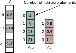
Figure 1: Sparse representation of a vector in the LIL format.

Using Fortran notation, a sparse array A(N,N) is represented by an integer array of indices A_ind(0:sm,N) and a real or double-precision array of values A_val(s_m,N). The access to a column is direct using the second index. A column is stored as the list of non-zero values in A_val and the corresponding row indices in A_ind (see figure 1). The elements at A_ind(0,:) contain the number of non-zero elements in the corresponding columns.

Using compiler directives, the floating-point arrays are aligned on a 512-byte boundary, and $s_{m}$ is constrained to be a multiple of 8 elements. In this way, all the columns of the array are properly aligned on the 256-bit boundary allowing aligned vector load and store instructions using both the SSE or the AVX instruction sets. Hence, each column starts whether at the beginning of a cache line, or at the middle of a cache line (in single precision).

If $s_{m}$ is set to a multiple of 512 double-precision elements, the columns are spaced by a multiple of 4 KiB. In this case, there will be conflict in the cache when loading two columns since they will have the same address in the cache. To avoid this so-called 4k-aliasing, we constrain $s_{m}$ to follow the rule

$$s_{m}=\alpha\times 512+24$$ (1)

For the largest system presented here, a box made of 504 896 water molecules (1.5 million atoms), the maximum value of the total resident memory was 982 GiB, which corresponds to an average of $\sim$ 680 KiB per atom.

III.2 Defining neighbouring lists of atoms and MOs (step I)

Two levels of localization or neighbouring are used in this work. Two atoms are always considered as neighbours, unless all the off-diagonal elements of the overlap matrix ${\bf S}$ and of the Fock/Kohn Sham matrix ${\bf H}$ involving one AO centered on each atom are zero. At the beginning of the program, an atomic neighbouring map is built and is used to avoid computing zero elements of ${\bf S}$ and ${\bf H}$ in the AO basis.

It is also convenient to use groups of localized MOs. This is done by generating an initial guess of MOs (see below) with non-zero coefficients on a limited number of AOs centered on atoms in the same region of space. During the orthonormalization and SCF process, MOs belonging to one group can of course delocalize and have coefficients on AOs centered on atoms belonging to another group. We however keep the initial group attribution of MOs during all the SCF process as the MOs are not expected to delocalize sufficiently to change the MO group attribution. Two groups are considered as neighbours if there exists a distance between one atom of the first group and an atom of the second one which is smaller than a given value (in practice we use 20 bohr). A map of MO group neighbours is built and we will assume that, in the MO basis, blocks of ${\bf H}$ and ${\bf S}$ involving non-neighbouring groups will always be zero. This assumption relies on the fact that as both occupied and virtual MOs are localized they are not expected to delocalize by more than 20 bohr during the SCF process. This assumption can be checked after the SCF has converged, and has not to be misinterpreted as a screening of long range $1/R$ interactions.

We now describe the procedure to build MO groups. Atomic orbitals centered on atoms that are geometrically far from each other have a zero overlap, and don’t interact through the Fock/Kohn Sham operator. All the atoms of the system are reordered such that atoms close to each other in the three-dimensional space are also close in the list of atoms. To achieve this goal, we use a constrained version of the k-means clustering algorithm.(kmeans, )

A set of $m$ centers (means) is first distributed evenly in the three-dimensional space. Every atom is linked to its closest center with the constraint that a center must be linked to no more than $N_{\rm link}$ atoms : If an atom can’t be linked to a center because the latter already has $N_{\rm link}$ linked atoms, the next closest center is chosen until an available center is found. Each center is then moved to the centroid of its connected atoms and the procedure is iterated until the average displacement of the centers is below a given threshold, or until a maximum number of iterations is reached (typically 100). Finally, the new list of atoms is built as the concatenation of the lists of atoms linked to each center.

Because of the constraint to have no more than $N_{\rm link}$ atoms attached to one center, the atom-to-center attribution depends on the order in which the atom list is explored and multiple solutions exist. This has no effect in the final energy since the definition of the neighbours depends on the atom-atom distances. However, it can have an impact on the computational time as the lists of neighbours can have different lengths. To cure this problem, the list of centers is randomly shuffled at every k-means iteration.

Each k-means attribution step is parallelized over the atoms. The $N_{\rm link}$ constraint introduces a coupling between the threads which is handled using an array of OpenMP locks: a lock is associated with each center, and the lock is taken by the thread before modifying its list of atoms and then released. The displacement of the centers is trivially parallelized over the centers, and this initialization step takes 2–5 % of the total wall time.

III.3 Initial guess of molecular orbitals (step II)

For each molecule of the system, a non-self-consistent calculation is performed. The molecular orbitals (MO) matrix ${\bf C}$ in the atomic orbitals (AO) basis set is built from the concatenation of all the lists of occupied MOs of each group and all the lists of virtual MOs of each group.

These MOs are not orthonormal but have the following properties:

• MOs are local: they have non-zero coefficients only on the basis functions that belong to the same molecule

• MOs belonging to the same molecule are orthonormal

• MOs $(i,j)$ belonging to MO groups that are not neighbours have a zero overlap and don’t interact: $({\bf C^{\dagger}SC})_{ij}=({\bf C^{\dagger}HC})_{ij}=0$

If the MOs don’t delocalize by more than 20 bohr, which was the case on all our benchmarks, the large off-diagonal blocks of zeros corresponding to the last point persist in the orthonormalization and SCF processes, so ${\bf C}$ always stays sparse.

The non-SCC calculations are parallelized over the molecules using a dynamic scheduling to keep a good load-balancing, and this initialization step takes less than 1% of the total wall time.

III.4 Orthonormalization of the molecular orbitals (step III)

The MOs are orthonormalized by diagonalizing iteratively the ${\bf C^{\dagger}SC}$ matrix. At this point, ${\bf C}$ is already stored in a sparse format.

1. ${\bf S}$ is computed (or read from memory) only in elements involving AOs of atomic neighbours

2. ${\bf C^{\dagger}SC}$ is computed

3. The MOs are normalized using diagonal elements of ${\bf C^{\dagger}SC}$

4. Combinations (approximate rotations) are performed between the pairs of MOs $(i,j)$ which involve the largest off-diagonal elements of the MO overlap matrix:

   $$C^{\prime}_{ki} = C_{ki}-\frac{C_{kj}({\bf C^{\dagger}SC})_{ij}}{2}$$

   $$C^{\prime}_{kj} = C_{kj}-\frac{C_{ki}({\bf C^{\dagger}SC})_{ij}}{2}$$

5. Return to step 3 until the largest off-diagonal element is below a given threshold

Note that, if the computational cost of building of the overlap matrix elements is comparable to reading it from the memory, it is suitable to compute the overlap matrix elements only when they are needed in the computation of ${\bf C^{\dagger}SC}$ to reduce the amount of storage.

The parallelization of the MO combinations (step d) is not trivial. If one combination of MOs $(i,j)$ is being performed by one thread, any combination of pairs of MOs involving either $i$ or $j$ can’t be performed simultaneously by another thread. First, we prepare an array of OpenMP locks, one lock for each MO. Then, we dress the list of orbital pairs $(i,j)$ to combine, those to which corresponds an off-diagonal element $|{\bf C^{\dagger}SC}|_{ij}\geq 10^{-3}\eta$, where $\eta$ is the largest off-diagonal element of $|{\bf C^{\dagger}SC}|$. The total length of the list is $N_{\rm pair}$. Each thread executes simultaneously the following steps:

1. Pick the first combination $(i,j)$ and go to step 3

2. Pick the next combination $(i,j)$

3. If the combination $(i,j)$ is already done, go to step 2

4. Try to take lock $L_{i}$ with OMP_TEST_LOCK. If not possible, go to step 2

5. Try to take lock $L_{j}$ with OMP_TEST_LOCK. If not possible, free lock $L_{i}$ and go to step 2

6. Combine $i$ and $j$ and mark $(i,j)$ as done

7. Free locks $L_{i}$ and $L_{j}$

8. Go back to step 2 until the end of the list is reached

9. Go back to step 1 until all combinations are done

The list of combinations is stored in an array, which can be large. Using the algorithm as presented explores many times the long list of combinations. After the first pass most of the combinations are done and looping over the whole array will spend a lot of time checking that a combination has already been done. An optimized approach consists in looping over only the first half of the array ($k\in[1,N_{\rm pair}/2]$). After a combination has been done, the elements $k$ and $k+N_{\rm pair}/2$ of the list are swapped. In this way, when the $N_{\rm pair}/2$ first elements have been explored, the first $N_{\rm pair}/2$ elements of the list are combinations to be done. Then, $N_{\rm pair}$ is set to $N_{\rm pair}/2$, and the procedure is repeated until $N_{\rm pair}<N_{\rm basis}$. Using this strategy allows to loop over only combinations to do and it avoids to check if a combination has already been done (loop over steps 2 and 3). At this point, there remains a few combinations to perform scattered in the array. Those last combinations are handled with the algorithm presented above (steps 1–9), but using blocking functions with OMP_SET_LOCK instead of the non-blocking OMP_TEST_LOCK. As most of the combinations have already been done, the probability of trying to lock simultaneously the same MO will be low and the locking steps will be occasional. Therefore, using blocking locks is relevant here since it will allow to perform only one traversal of the array to complete the remaining combinations.

The orthonormalization takes 40–50% of the total wall time. Half of the time is spent in the MO rotations and the other half is spent in the computation of ${\bf C^{\dagger}SC}$ which is discussed in detail below.

III.5 Partial diagonalization of the Fock/Kohn Sham matrix (step IV)

The wave function is invariant with respect to unitary transformations among doubly occupied orbitals or among virtual orbitals. Therefore, the full diagonalization of ${\bf H}$ is not necessary to obtain the SCF minimum energy and properties. It is sufficient to annihilate only the matrix elements of the Fock/Kohn Sham matrix expressed in the MO basis involving one occupied and one virtual orbital. To do that, we use an approach similar to the orthonormalization procedure: we apply Jacobi rotations between in the occupied and virtual orbitals, as proposed by Stewart.(stewart, ) To preserve the orthonormality of the MOs, the orbitals are combined using an accurate rotation but with an approximate angle.

1. Compute ${\bf H}$ only in elements involving AOs of neighbouring atoms

2. Compute ${\bf C^{\dagger}HC}$ as explained in next section

3. Rotate the pair of MOs $(i,j)$ which involves the largest off-diagonal element:

   $$p = \frac{({\bf C^{\dagger}HC})_{ii}-({\bf C^{\dagger}HC})_{jj}}{2({\bf C^{\dagger}HC})_{ij}}$$

   $$t = \left(p+\operatorname{sgn}(p)\sqrt{1+p^{2}}\right)^{-1}$$

   $$c = \left(1+t^{2}\right)^{-1/2}$$

   $$s = tc$$

   $$C^{\prime}_{ki} = cC_{ki}+sC_{kj}$$

   $$C^{\prime}_{kj} = -sC_{kj}+cC_{ki}$$

4. Return to step 3 until the largest off-diagonal element is below a given threshold or if the number of rotations is equal to 10 times the number of occupied MOs.

As mentioned for the orthonormalization, it can be suitable to compute the elements of the Fock/Kohn Sham matrix directly when needed at the second step to avoid the storage of a matrix.

Avoiding to perform occupied-occupied and virtual-virtual rotations keeps both the occupied and virtual MOs localized during the optimization.(angeli, ; maynau, ) In this way, the ${\bf C}$ matrix stays sparse. The ${\bf C^{\dagger}HC}$ matrix is displayed in figure 2. As the matrix is symmetric and only the occupied-virtual rotations are considered, only one occupied-virtual block is computed for the orbital rotations, appearing in white on the figure. This block can be divided in sub-blocks using the MO groups definition.

The parallelization of the rotations is implemented such that one orbital can never be rotated simultaneously by two threads : each thread performs a rotation in a block of the occupied-virtual elements. The figure shows the outer loop iterations. On the first iteration, the threads perform rotations in all the blocks labeled by 1. After a synchronization, on the second iteration they perform rotations in the blocks labeled by 2, etc. Blocks between non neighbouring MO groups are not considered for the rotation process. Let us mention that in practice the occupied-virtual ${\bf C^{\dagger}HC}$ block is computed and stored in a sparse format.

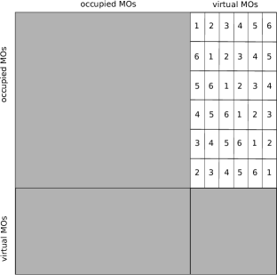
Figure 2: Representation of the ${\bf C^{\dagger}HC}$ matrix. Only one off-diagonal block is annihilated by pseudo-Jacobi rotations. The numbers identify iterations. On the first iteration, blocks labeled by 1 are annihilated in parallel, etc

The time spent in the MO rotations represents 3–6% of the total wall time. The bottleneck is the calculation of ${\bf C^{\dagger}HC}$. Adding the timing of ${\bf C^{\dagger}HC}$ yields 33–40% of the total wall time.

III.6 Computation kernel for the matrix products ${\bf C}^{\dagger}{\bf XC}$ (steps III and V)

From the two previous sections, it appears that the main hot spot is the computation of double sparse matrix products of the form ${\bf C}^{\dagger}{\bf XC}$ where ${\bf X}={\bf S}$ for the orthonormalization part and ${\bf X}={\bf H}$ for the diagonalization part. We explain here how this step is performed taking advantage of the sparsity of matrices ${\bf C}$, ${\bf H}$ and ${\bf S}$.

In another work, an efficient dense$\times$sparse matrix product subroutine for small matrices was implemented in the QMC=Chem quantum Monte Carlo software.(qmcchem, ) These matrix products are hand-tuned for Intel Sandy-Bridge and Ivy-Bridge micro-architectures, and have reached more than 60% of the peak performance of a CPU core. To obtain such results, some programming constraints are necessary and are detailed in the next section.

In what follows, large sparse$\times$sparse matrix products are performed as a collection of small dense$\times$sparse products avoiding the zero-blocks connecting non-neighbouring MO groups.

III.6.1 Small dense$\times$sparse matrix products

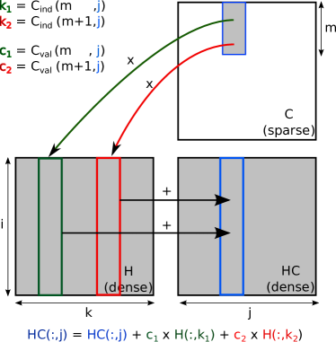
Figure 3: Dense$\times$sparse matrix product.

Let us recall the dense$\times$sparse matrix products of Ref (qmcchem, ). In the multiplication routine, the loops are reordered such that vectorization is possible, giving a dense matrix in output (see figure 3). As the innermost loop has a small number of iterations, the following constraints are mandatory to obtain performance:

• All arrays have to be 32-byte aligned using compiler directives

• The leading dimensions of arrays should be multiples of 8 elements such that all the columns are 32-byte aligned

Without these constraints, the compiler will generate both the scalar and the vector version of the loop, and the scalar version will be used as long as the 32-byte alignment is not reached (peeling loop) or if a register of 4 double precision or 8 single precision elements cannot be filled (tail loop). In such a case, a 16-iteration loop in single precision will perform 8 scalar loop cycles and one vector loop cycle. Using the alignment and padding constraints, the compiler can produce 100% vector instructions with no branching and will execute 2 vector loop cycles unrolled by the compiler, resulting in a speedup of more than 5. Note that these constraints contribute to the choice of the memory layout for sparse matrices explained previously.

III.6.2 Computation of ${\bf C^{\dagger}XC}$

For each thread, the algorithm is the following:

1. Compute 16 contiguous columns of ${\bf XC}$ in a dense representation

2. Transpose the result to obtain 16 rows of ${\bf C^{\dagger}X}$

3. Multiply on the right by ${\bf C}$ to obtain 16 rows of ${\bf C^{\dagger}XC}$

4. As ${\bf C^{\dagger}XC}$ is symmetric, transpose the dense 16 rows of ${\bf C^{\dagger}XC}$ into a sparse representation of 16 columns of ${\bf C^{\dagger}XC}$

5. Iterate until all the columns of ${\bf C^{\dagger}XC}$ are built

In step 1, dense$\times$sparse matrix products are performed using only the $16\times 16$ blocks of ${\bf X}$ containing at least one non-zero element. This exploits the sparse character of ${\bf X}$ by avoiding large blocks of zeros using the atomic neighbour list. The $16\times 16$ shape of the arrays is constant and known at compile time, and all the columns of the $16\times 16$ arrays are 32-byte aligned. This permits the compiler to remove the peeling and tail loops and generate a fully vectorized code.

The 16 dense columns of ${\bf XC}$ are not stored as a ($N_{\rm basis}$,16)-array, but are instead represented as an array of $16\times 16$ matrices: the dimension of the array is $(16,16,\lfloor N_{\rm basis}/16\rfloor+1)$. The reason for this layout is twofold. First, the result of ${\bf XC}$ is written linearly into memory. The spatial locality in the cache is improved and this reduces the traffic between the caches and the main memory. Secondly, step 2 can be performed very fast since the transposition of ${\bf XC}$ consists in $\lfloor N_{\rm basis}/16\rfloor+1$ in-place transpositions of contiguous $16\times 16$ matrices. Using the ($N_{\rm basis}$,16) layout, the transposition would involve memory accesses distant by $N_{\rm basis}$ elements suffering from a high memory latency overhead for large systems since the hardware prefetchers prefetch data only up to a memory page boundary. Using our layout, the transposition is always memory-bandwidth bound as each $16\times 16$ transposition occurs in the L1 cache and the next $16\times 16$ matrix is automatically prefetched.

In step 3, the dense$\times$sparse product is performed using only the columns of ${\bf C}$ belonging to MO groups which are neighbours of the MO groups to which the 16 rows of ${\bf C^{\dagger}X}$ belong. Again, the loop count of the inner-most loop is 16 and this part is fully vectorized as all the columns of the arrays are properly aligned.

III.6.3 Parallel efficiency

Figure 4: Parallel speed-up of ${\bf C^{\dagger}XC}$ as a function of the number of water molecules obtained on the dual-socket server. The speed-ups were renormalized to remove the effect of the turbo feature. The 32 threads results were obtained using Hyperthreading (2 threads per physical core).

Figure 5: Wall time of ${\bf C^{\dagger}XC}$ as a function of the number of water molecules obtained on the dual-socket server. The 32 threads results were obtained using Hyperthreading (2 threads per core).

The parallel speedup curve of the ${\bf C^{\dagger}XC}$ products measured on the dual-socket server is shown in figure 4. For small sizes, the speed-up is nearly optimal (the perfect value of 16 obtained here is fortunate, since measuring very small wall-times contains large uncertainties). This can be explained by the fact that most of the matrices can fit in the level 3 cache. Then, as the size of the C matrix increases, more and more pressure is made between the level 3 cache and the memory, as every core has to read the whole ${\bf C}$ matrix when multiplying the 16-rows with ${\bf C}$. The latency of data access to C increases accordingly and the processor cores can’t be kept busy. This is confirmed by the fact that Hyperthreading improves the parallel efficiency by giving some work to a core for one thread while another thread is stalled. The speed-up converges to a limit of 11 for a 16-core machine. The wall time curve of figure 5 shows a scaling with the number of atoms of ${\cal O}(N^{1.47})$. The scaling is not linear, because of the non-uniformity of the memory latencies.

III.7 Specific implementation for DFTB

We now turn to the specific implementation of the previously described algorithm for density functional based tight binding (DFTB), an approximate DFT scheme.(dftb1, ; dftb2, ; scc-dftb, ; elstner2006scc, ; frauenheim00, ; frauenheim02, ; augusto09, ) The electronic problem is only solved for valence electrons and molecular orbitals are expressed in a minimal atomic basis set. The DFTB Kohn-Sham (KS) matrix is:

$$H_{\mu\nu}=H^{0}_{\mu\nu}+\frac{1}{2}S_{\mu\nu}\sum_{\xi}(\gamma_{\alpha\xi}+\gamma_{\beta\xi})\Delta q_{\xi}$$ (2)

$H^{0}_{\mu\nu}$ is the KS matrix element between orbitals $\mu$ of atom $\alpha$ and $\nu$ of atom $\beta$ at a reference density. This value is usually interpolated from pre-calculated DFT curves (the so-called Slater Koster tables(SlaterKoster54, )). One-site $\gamma_{\alpha\alpha}$ are obtained from Hubbard parameters and inter-atomic $\gamma_{\alpha\xi}$ depend on the distances between atoms $\alpha$ and $\xi$, and contain the long range $1/R$ Coulomb interaction. $\Delta q_{\xi}=q_{\xi}-q^{0}_{\xi}$ is the charge fluctuation of atom $\xi$ calculated with the Mülliken analysis scheme:

$$q_{\xi}=\sum_{i}^{N_{\rm MOs}}n_{i}\sum_{\nu}^{N_{\rm AOs}}\sum_{\mu\in\xi}C_{i\mu}C_{i\nu}S_{\mu\nu}=\sum_{\nu}^{N_{\rm AOs}}\sum_{\mu\in\xi}P_{\mu\nu}S_{\mu\nu}$$ (3)

where ${\bf P}$ is the density matrix in the AO basis set.

Computing the atomic Mülliken population of Eq. 3 could be an expensive part that has to be efficiently parallelized. The parallelization can be done either on the MOs (one thread deals with a subset of MOs and computes their contributions to the atomic populations of the whole system) or on the atomic population (one thread computes the atomic population of some atoms arising from all the MOs). The first scheme is limited by storing data whereas the second one is limited by reading data. Storing data in memory is more costly than reading data, so the second scheme was chosen. An acceleration can be achieved considering the spatial localization of molecular orbitals (only a limited number of MOs contribute to the population of a given atom). For each atom $\alpha$ we dress the list of the indexes of MOs having a non-zero contribution on atom $\alpha$. Then, we compute a set of rows of the density matrix $P_{\mu\in\alpha,\nu}=\sum_{i}C_{i\mu}C_{i\nu}$, where $\nu$ is such that $S_{\mu,\nu}\neq 0$ (using the atomic neighbours list), and the sum over MOs $i$ only runs on the MOs listed as contributors on atom $\alpha$. $q_{\xi}$ is then computed from equation Eq. 3. The calculation of the charges $q_{\xi}$ takes typically 3% of the total wall time, and the observed scaling is ${\cal O}(N^{1.1})$. Note that we limit the number of threads to a maximum of 16 in this part. Indeed, this section is extremely sensitive to memory latency as the arithmetic intensity is very low. Using more than 16 threads would need inter-blade communications on the Altix UV which always hurt the performance for this particular section.

From the computational point of view, it is better to compute first a vector $Q_{\alpha}=\sum_{\xi}\gamma_{\alpha\xi}\Delta q_{\xi}$ to rewrite Eq. 2 as:

$$H_{\mu\nu}=H^{0}_{\mu\nu}+\frac{1}{2}S_{\mu\nu}(Q_{\alpha}+Q_{\beta})$$ (4)

The computation of the $Q_{\alpha}$ values requires ${\cal O}(N^{2})$ operations. This term contains actually the long range $1/R$ contributions to the Coulomb energy and a linear scaling on this part could only be reached at the price of approximations. We decided not to screen these long-range contributions in order to keep the same results as those one would obtain from a standard diagonalization scheme, the computational cost remaining acceptable (less than 20% of the total wall time for the largest systems of our benchmarks).

IV Results obtained on the whole scheme

IV.1 Sparsity and numerical accuracy

In the deMon-Nano program, the convergence criterion of the SCF procedure is based on the largest fluctuation of the Mülliken charge :

$$\delta q_{\max}=\max_{i}|q_{i}^{(n)}-q_{i}^{(n-1)}|$$ (5)

where $q_{i}^{(n)}$ denotes the Mülliken charge of atom $i$ at SCF iteration $n$. As this criterion is local, it ensures that all the different regions of the system have converged to a desired quality, as opposed to a criterion based on the total energy of the system which is global. We define the sparse threshold $\epsilon$ as a quantity used to adjust the sparsity of the MO matrices. $\epsilon$ is set ten times lower than the target SCF convergence criterion $\delta q_{\max}$, such that if more precision is requested for the SCF, the matrices become less and less sparse. In the limit where the requested SCF convergence threshold is zero, the matrices are dense and the exact result is recovered.

Once the initial guess is done, the initial MOs are improved by running an SCF with very loose thresholds: $\epsilon\leq 10^{-3}$ and $\delta q_{\max}\leq 10^{-1}$ a.u. The calculation is then started using the thresholds given by the user in input. In what follows, the thresholds were $\epsilon\leq 10^{-6}$ and $\delta q_{\max}\leq 10^{-5}$ a.u. Typically 8 SCF iterations were needed to reach a convergence of $\delta q_{\max}\leq 10^{-1}$ a.u., and 9–13 additional iterations were necessary for $\delta q_{\max}\leq 10^{-5}$ a.u.

Figure 6: Percentage of non-zero elements during the execution of the program.

The orthonormalization needs to be very accurate, so all the orthonormalization procedure is run in double precision. After each rotation of pairs of MOs, the MO coefficients ${\bf C}_{ki}$ such that $|{\bf C}_{ki}|<10^{-3}\epsilon$ are set to zero. This cut-off is chosen much smaller than $\epsilon$ to ensure that the quality of the orthonormalization will be sufficient. However, this leads to an increase of the number of non-zero elements in ${\bf C}$ (see figure 6). The orthonormalization is considered converged when the absolute value of the largest off-diagonal element of ${\bf C^{\dagger}SC}$ is lower than $\epsilon/100$.

The partial diagonalization of ${\bf H}$ does not need to be as precise as the orthonormalization, so single precision is used to accelerate the calculation of ${\bf C^{\dagger}HC}$. A threshold of $\epsilon$ is applied to the matrix elements of ${\bf H}$, and to the elements of ${\bf C}$ after a rotation of MOs. This larger cut-off increases the sparsity of ${\bf C}$, but degrades the orthonormality of the MOs. To cure this latter problem, an additional orthonormalization step among only the occupied MOs is performed after the SCF has converged.

Table 1: Total energies in a.u. obtained with the full diagonalization using the Intel MKL implementation of the LAPACK library(lapack, ) ($E_{\rm LAPACK}$) or the implementation proposed in this work ($E$). $N$ is the number of water molecules.

$N$	$E_{\rm LAPACK}$	$E$	$\frac{E-E_{\rm LAPACK}}{E_{\rm LAPACK}}$
$\delta q_{\max}=10^{-5}$
184	-749.63938702	-749.63938696	8.0 10-11
368	-1499.33163492	-1499.33163479	8.7 10-11
736	-2998.74237166	-2998.74237136	1.0 10-10
1472	-5997.78267988	-5997.78267920	1.1 10-10
2208	-8996.78192470	-8996.78192364	1.2 10-10
3312	-13495.30553928	-13495.30553764	1.2 10-10
$\delta q_{\max}=10^{-6}$
184	-749.63942605	-749.63942605	$<$ 6.7 10-12
368	-1499.33168960	-1499.33168960	$<$ 3.3 10-12
736	-2998.74251247	-2998.74251247	$<$ 1.7 10-12
1472	-5997.78296964	-5997.78296962	3.3 10-12
2208	-8996.78231327	-8996.78231325	2.2 10-12
3312	-13495.30617832	-13495.30617828	3.0 10-12

The total energies obtained with the divide and conquer LAPACK routine DSYGVD are compared to our implementation in table 1 with different SCF convergence criteria. One can first remark that as the convergence criterion of the SCF procedure gets lower, the error due to our implementation decreases as $\epsilon$ decreases accordingly. Moreover, the difference in total energies between the reference LAPACK result and our implementation is orders of magnitudes below the error due to the lack of convergence of the SCF procedure. The absolute error per water molecule is below $2~{}10^{-10}$ using $\delta q_{\max}=10^{-5}$, and around $3~{}10^{-12}$ for $\delta q_{\max}=10^{-6}$.

IV.2 Parallel efficiency and scaling

In this section, the time values correspond to the timing of the whole program, as obtained by the time UNIX tool.

Figure 7: Parallel speedup as a function of the number of water molecules on the dual-socket server. The data were renormalized to remove the effect of the turbo feature. The 32 threads results were obtained using Hyperthreading (2 threads per core).

Figure 8: Parallel speedup as a function of the number of water molecules obtained on the Altix UV machine. The reference is one 16-core blade.

Figure 9: Total wall time (s) as a function of the number of water molecules obtained on the dual-socket server. The 32 threads results were obtained using Hyperthreading (2 threads per core).

Figure 10: Total wall time (s) as a function of the number of water molecules obtained on the Altix UV machine.

Figure 7 shows the parallel speed-up of the program on the dual-socket server. When using all the 16 available physical cores of the machine, the parallel efficiency converges quickly to value between 11 and 12. One can remark that Hyperthreading improves the parallel efficiency. Indeed, as the memory latencies are the bottleneck, the CPU core can be kept busy for one thread while another thread waits for data. On the Altix UV (figure 8), the speed-up is presented as a function of the number of 16-core blades. Indeed, the important NUMA effects show up when using more than one blade, since the inter-blade memory latency is significantly higher than the intra-blade latency by a factor between 2 and 5. This explains why the parallel efficiency is disappointing on the Altix UV: a speed-up close to 2 is obtained with 8 blades for small systems. However, when the systems is so large that the total memory can’t fit on a single blade, the 16-core reference suffers from a degradation of performance due to the NUMA effects, so the comparison becomes more fair between the single-blade and the 8-blade runs, and the parallel speed-up is much more acceptable, around 5.

From figures 9 and 10, the scaling of the program as a function of the number of atoms is ${\cal O}(N^{1.7})$ on the dual-socket server, and ${\cal O}(N^{1.8})$ on the Altix UV. The global scaling is not linear. This is first due to the non-uniformity of the memory access: the code is faster with smaller memory footprints since the latencies are smaller. Secondly, in the expression of the Fock matrix elements (Eqs. 2 and 4), for each atom one has to compute the Coulomb contributions with all the other atoms. We chose not to truncate the $1/R$ function in order to keep a good error control on the final energies, and this results in a quadratic scaling with the number of atoms appearing for large systems (10% of the total time for 33 120 molecules on the dual-socket server, and 18% for 504 896 molecules on the Altix UV).

Figure 11: Average CPU time (s) per atom with increasing numbers of water molecules.

The CPU time per atom is given in figure 11. A similar benchmark was presented with a linear-scaling approach in the density-matrix framework.(cp2k, ) The authors reported roughly $10$–$19$ CPU seconds per atom for systems with $50~{}10^{3}$–$1.1~{}10^{6}$ atoms. It is difficult to compare quantitatively our timings with theirs, because the method is different, molecular geometries are different and the hardware on which the code ran is different. However, one can tell that our implementation gives CPU timings in the same order of magnitude. Another important point is that these authors used an MPI-based implementation, where they report roughly 20% of the time spent in MPI communication routines. Indeed, as linear-scaling techniques are memory-latency bound, obtaining an efficient MPI implementation is a challenge since MPI communications have a higher latency than memory accesses, even with low-latency network hardware (Infiniband). Remark that our large simulations on the Altix UV are very efficient because hardware prefetching occurs even when the target memory is located on a distant blade. Therefore, the hardware makes automatically asynchronous inter-blade communication to further reduce the memory latency bottleneck, which is not trivial to implement in a portable MPI framework. This confirms also that our choice to defer the distributed parallelism to coarser graining is a good choice.

V Summary and future work

We have presented an efficient OpenMP implementation enabling MO-based SCC-DFTB for very large molecular systems. As linear-scaling techniques reduce the arithmetic intensity, these algorithms are inevitably memory-latency bound. Our implementation was designed to minimize the effect of this bottleneck. We have shown that we were able to run a calculation on more than 1.5 million atoms (504 896 water molecules) with a very good efficiency on 128 cores of an SGI Altix UV machine, a machine with very strong NUMA effects and memory latencies that can be up to ten times larger than the memory latencies of a standard desktop computer. The program is even more efficient for smaller systems (1 000–100 000 molecules), the range which is the most suited to practical applications of DFTB. This aspect will permit to run much longer molecular dynamics trajectories on medium-sized systems. This OpenMP-only implementation makes it possible to run simulations with up to 100 000 atoms using standard servers, without the need of expensive low-latency network hardware. The errors introduced by our approximations were shown to be below the error of the SCF convergence threshold, which makes us trust our results for simulations with more than a million of atoms, a domain where it is impossible to verify the validity of the result using an exact diagonalization. The next step of this project will be to implement distributed parallelism to enable large scale Monte Carlo simulations of biological molecules in water.

Acknowledgments. The authors would like to thank ANR for support under Grant No ANR 2011 GASPARIM, ANR PARCS, This work was supported by “Programme Investissements d’Avenir” under the program ANR-11-IDEX-0002-02 reference ANR-10-LABX-0037-NEXT, CALMIP and Equipex Equip$@$Meso for computational facilities.

References

- (1) Pierre Hohenberg and Walter Kohn. Inhomogeneous electron gas. Physical review, 136(3B):B864, 1964.
- (2) Walter Kohn and Lu Jeu Sham. Self-consistent equations including exchange and correlation effects. Physical Review, 140(4A):A1133, 1965.
- (3) Adam HR Palser and David E Manolopoulos. Canonical purification of the density matrix in electronic-structure theory. Physical Review B, 58:75524–12711, 1998.
- (4) Anders MN Niklasson, CJ Tymczak, and Matt Challacombe. Trace resetting density matrix purification in o (n) self-consistent-field theory. The Journal of chemical physics, 118(19):8611–8620, 2003.
- (5) Anders MN Niklasson, Valéry Weber, and Matt Challacombe. Nonorthogonal density-matrix perturbation theory. The Journal of chemical physics, 123(4):044107, 2005.
- (6) R. McWeeny. Some recent advances in density matrix theory. Reviews of Modern Physics, 32(2):335, 1960.
- (7) Matt Challacombe. A simplified density matrix minimization for linear scaling self-consistent field theory. The Journal of chemical physics, 110(5):2332–2342, 1999.
- (8) Daniel K Jordan and David A Mazziotti. Comparison of two genres for linear scaling in density functional theory: Purification and density matrix minimization methods. The Journal of chemical physics, 122(8):084114, 2005.
- (9) Emanuel H Rubensson, Elias Rudberg, and Paweł Sałek. Density matrix purification with rigorous error control. The Journal of chemical physics, 128(7):074106, 2008.
- (10) Elias Rudberg and Emanuel H Rubensson. Assessment of density matrix methods for linear scaling electronic structure calculations. Journal of Physics: Condensed Matter, 23(7):075502, 2011.
- (11) Elias Rudberg, Emanuel H Rubensson, and Paweł Sałek. Kohn-sham density functional theory electronic structure calculations with linearly scaling computational time and memory usage. Journal of Chemical Theory and Computation, 7(2):340–350, 2010.
- (12) X-P Li, RW Nunes, and David Vanderbilt. Density-matrix electronic-structure method with linear system-size scaling. Physical Review B, 47(16):10891, 1993.
- (13) DR Bowler and MJ Gillan. Density matrices in electronic structure calculations: theory and applications. Computer physics communications, 120(2):95–108, 1999.
- (14) Xiaosong Li, John M Millam, Gustavo E Scuseria, Michael J Frisch, and H Bernhard Schlegel. Density matrix search using direct inversion in the iterative subspace as a linear scaling alternative to diagonalization in electronic structure calculations. The Journal of chemical physics, 119(15):7651–7658, 2003.
- (15) John M Millam and Gustavo E Scuseria. Linear scaling conjugate gradient density matrix search as an alternative to diagonalization for first principles electronic structure calculations. The Journal of chemical physics, 106(13):5569–5577, 1997.
- (16) Satrajit Adhikari and Roi Baer. Augmented lagrangian method for order-n electronic structure. The Journal of chemical physics, 115(1):11–14, 2001.
- (17) Andrew D Daniels, John M Millam, and Gustavo E Scuseria. Semiempirical methods with conjugate gradient density matrix search to replace diagonalization for molecular systems containing thousands of atoms. The Journal of chemical physics, 107(2):425–431, 1997.
- (18) Linda Hung and Emily A Carter. Accurate simulations of metals at the mesoscale: Explicit treatment of 1 million atoms with quantum mechanics. Chemical Physics Letters, 475(4):163–170, 2009.
- (19) Joost VandeVondele, Urban Borštnik, and Jürg Hutter. Linear scaling self-consistent field calculations with millions of atoms in the condensed phase. Journal of Chemical Theory and Computation, 8(10):3565–3573, 2012.
- (20) Steven L Dixon and Kenneth M Merz Jr. Fast, accurate semiempirical molecular orbital calculations for macromolecules. The Journal of chemical physics, 107(3):879–893, 1997.
- (21) JJP Stewart, P Csaszar, and P Pulay. Fast semiempirical calculations. Journal of Computational Chemistry, 3(2):227–228, 1982.
- (22) T. Heine, M. Rapacioli, S. Patchkovskii, J. Frenzel, A. Koster, P. Calaminici, H. A. Duarte, S. Escalante, R. Flores-Moreno, A. Goursot, J. Reveles, D. Salahub, and A. Vela. demon-nano experiment 2009. http://physics.jacobs-university.de/theine/research/deMon/.
- (23) Dirk Porezag, Th Frauenheim, Th Köhler, Gotthard Seifert, and R Kaschner. Construction of tight-binding-like potentials on the basis of density-functional theory: Application to carbon. Physical Review B, 51(19):12947, 1995.
- (24) G Seifert, D Porezag, and Th Frauenheim. Calculations of molecules, clusters, and solids with a simplified lcao-dft-lda scheme. International journal of quantum chemistry, 58(2):185–192, 1996.
- (25) Marcus Elstner, Dirk Porezag, G Jungnickel, J Elsner, M Haugk, Th Frauenheim, Sandor Suhai, and Gotthard Seifert. Self-consistent-charge density-functional tight-binding method for simulations of complex materials properties. Physical Review B, 58(11):7260, 1998.
- (26) Th Frauenheim, G Seifert, M Elsterner, Z Hajnal, G Jungnickel, D Porezag, S Suhai, and R Scholz. A self-consistent charge density-functional based tight-binding method for predictive materials simulations in physics, chemistry and biology. physica status solidi(b), 217(1):41–62, 2000.
- (27) Thomas Frauenheim, Gotthard Seifert, Marcus Elstner, Thomas Niehaus, Christof Köhler, Marc Amkreutz, Michael Sternberg, Zoltán Hajnal, Aldo Di Carlo, and Sándor Suhai. Atomistic simulations of complex materials: ground-state and excited-state properties. Journal of Physics: Condensed Matter, 14(11):3015, 2002.
- (28) Augusto F Oliveira, Gotthard Seifert, Thomas Heine, and Hélio A Duarte. Density-functional based tight-binding: an approximate dft method. Journal of the Brazilian Chemical Society, 20(7):1193–1205, 2009.
- (29) Balint Aradi, Ben Hourahine, and Th Frauenheim. Dftb+, a sparse matrix-based implementation of the dftb method. The Journal of Physical Chemistry A, 111(26):5678–5684, 2007.
- (30) Haiyan Liu, Marcus Elstner, Efthimios Kaxiras, Thomas Frauenheim, Jan Hermans, and Weitao Yang. Quantum mechanics simulation of protein dynamics on long timescale. Proteins: Structure, Function, and Bioinformatics, 44(4):484–489, 2001.
- (31) Timothy J Giese, Haoyuan Chen, Thakshila Dissanayake, George M Giambaşu, Hugh Heldenbrand, Ming Huang, Erich R Kuechler, Tai-Sung Lee, Maria T Panteva, Brian K Radak, et al. A variational linear-scaling framework to build practical, efficient next-generation orbital-based quantum force fields. Journal of chemical theory and computation, 9(3):1417–1427, 2013.
- (32) Leonardo Dagum and Ramesh Menon. Openmp: an industry standard api for shared-memory programming. Computational Science & Engineering, IEEE, 5(1):46–55, 1998.
- (33) William Gropp, Ewing Lusk, Nathan Doss, and Anthony Skjellum. A high-performance, portable implementation of the mpi message passing interface standard. Parallel computing, 22(6):789–828, 1996.
- (34) David R Kincaid, John R Respess, David M Young, and Rober R Grimes. Algorithm 586: Itpack 2c: A fortran package for solving large sparse linear systems by adaptive accelerated iterative methods. ACM Transactions on Mathematical Software (TOMS), 8(3):302–322, 1982.
- (35) Rami Melhem and Dennis Gannon. Toward efficient implementation of preconditioned conjugate gradient methods on vector supercomputers. International Journal of High Performance Computing Applications, 1(1):70–98, 1987.
- (36) Iain S Duff, Albert Maurice Erisman, and John Ker Reid. Direct methods for sparse matrices. Clarendon Press Oxford, 1986.
- (37) James MacQueen et al. Some methods for classification and analysis of multivariate observations. In Proceedings of the fifth Berkeley symposium on mathematical statistics and probability, volume 1, pages 281–297. California, USA, 1967.
- (38) Celestino Angeli, Stefano Evangelisti, Renzo Cimiraglia, and Daniel Maynau. A novel perturbation-based complete active space–self-consistent-field algorithm: Application to the direct calculation of localized orbitals. The Journal of chemical physics, 117(23):10525–10533, 2002.
- (39) Daniel Maynau, Stefano Evangelisti, Nathalie Guihéry, Carmen J Calzado, and Jean-Paul Malrieu. Direct generation of local orbitals for multireference treatment and subsequent uses for the calculation of the correlation energy. The Journal of chemical physics, 116(23):10060–10068, 2002.
- (40) Anthony Scemama, Michel Caffarel, Emmanuel Oseret, and William Jalby. Quantum monte carlo for large chemical systems: Implementing efficient strategies for petascale platforms and beyond. Journal of computational chemistry, 34(11):938–951, 2013.
- (41) M Elstner. The scc-dftb method and its application to biological systems. Theoretical Chemistry Accounts, 116(1-3):316–325, 2006.
- (42) John C Slater and George F Koster. Simplified lcao method for the periodic potential problem. Physical Review, 94(6):1498, 1954.
- (43) Edward Anderson, Zhaojun Bai, Jack Dongarra, A Greenbaum, A McKenney, Jeremy Du Croz, S Hammerling, James Demmel, C Bischof, and Danny Sorensen. Lapack: A portable linear algebra library for high-performance computers. In Proceedings of the 1990 ACM/IEEE conference on Supercomputing, pages 2–11. IEEE Computer Society Press, 1990.