Memory effects in chaotic advection of inertial particles

Abstract

A systematic investigation of the effect of the history force on particle advection is carried out for both heavy and light particles. General relations are given to identify parameter regions where the history force is expected to be comparable with the Stokes drag. As an illustrative example, a paradigmatic two-dimensional flow, the von Kármán flow is taken. For small (but not extremely small) particles all investigated dynamical properties turn out to heavily depend on the presence of memory when compared to the memoryless case: the history force generates a rather non-trivial dynamics that appears to weaken (but not to suppress) inertial effects, it enhances the overall contribution of viscosity. We explore the parameter space spanned by the particle size and the density ratio, and find a weaker tendency for accumulation in attractors and for caustics formation. The Lyapunov exponent of transients becomes larger with memory. Periodic attractors are found to have a very slow, $t^{-1/2}$ type convergence towards the asymptotic form. We find that the concept of snapshot attractors is useful to understand this slow convergence: an ensemble of particles converges exponentially fast towards a snapshot attractor, which undergoes a slow shift for long times.

1 Introduction

The advection of small, rigid, finite-size particles has been studied recently in several setups because it plays an important role in many environment-related phenomena ranging from atmospheric science and oceanography to astrophysics (for reviews see [1, 2, 3]). For example, inertial particles are important in cloud microphysics [4, 5], planet formation [6], and aggregation and fragmentation processes in fluid flows [7, 8, 9]. A particularly interesting aspect is the advection of such particles in chaotic flows where experimental results [10, 11] are available by now. Applications can be for example the forecasting of pollutant transport for homeland defense [12, 7] and the localization of a toxin or biological pathogen spill (e.g. anthrax) from outbreaks in a street canyon [13].

Due to the drag acting on the particles, the Hamiltonian passive advection problem is converted into a dissipative problem which can have attractors. Correspondingly, inertial particles can have the tendency to accumulate in certain regions of the flow [14] (a phenomenon termed preferential concentration). A characteristic feature in comparison with the dynamics of ideal tracers is the appearance of caustics [4, 15], i.e., the intersection of different branches of the chaotic sets in the configuration space. This is a consequence of the fact that what we see is a projection of the full pattern of the high-dimensional phase space to the configuration space of the fluid. The main relevance of the existence of caustics is that the probability of collisions of particles becomes enhanced in such regions of the flow.

The basic equation of motion for small spherical particles in a viscous fluid describable in the Stokes regime is given by the Maxey-Riley equations [16, 17]. Its precise form contains an integral, also called the history force, which describes the diffusion of vorticity around the particle during its full time history. The kernel of this integral is therefore proportional to the power -1/2 of the elapsed time.

The origin of such a kernel can perhaps best be seen in the problem of an infinitely large plate moving in a rather viscous fluid. If the plate starts at time zero with a sudden change in the velocity which is then kept constant, in Stokes approximation, one solves the diffusion equation for the velocity field. The solution contains a prefactor $1/\sqrt{t}$. For the case of a general motion of the plate, one imagines to break up the problem in a set of jumps in the plate’s velocity at different times $\tau$. Each such jump contributes a factor to the flow velocity at time $t$ proportional to $1/\sqrt{t-\tau}$ multiplied by the velocity jump. In a continuous time picture, the result for the shear stress on the plate is proportional to an integral from zero to $t$ of the plate’s acceleration at time $\tau$ multiplied by the kernel $1/\sqrt{t-\tau}$ (see Landau-Lifschitz [19], paragraph 24). For the motion of a spherical particle in a viscous flow it were Boussinesq and Basset (at the end of the 19th century) who pointed out the appearance of such a history force (for historical details see [20]). This force is therefore sometimes called the Boussinesq-Basset or the Basset force (we use the term history force). The equation of motion of a moving sphere in a fluid at rest was already given in Landau-Lifschitz ([19], problem 7 to paragraph 24). The precise form of the equation in a moving fluid [16, 17, 18], i.e., equation (2) or (6), was, however, established only a century after the first works of Boussinesq and Basset.

The history force renders the advection equation of inertial particles to be an integro-differential equation. Because of this difficulty, the memory represented by this integral term was neglected in the majority of papers on chaotic advection of inertial particles.

In non-chaotic flows, the history force was shown to have important effects [21, 22, 23, 24, 25]. A particularly interesting example is an experiment [26, 27] which points out the determining importance of memory in the motion of microbubbles propelled by ultrasound. In this setting the trajectories, and a surprising destabilization of these (in spite of rather strong dissipation), can be understood only when the history force is taken into account. A very recent experiment with suspended particles indicates the importance of the history force also in the phenomenon of Brownian motion [28]. Within a perturbative treatment restricted to the limit of very weak inertia, it has been found that the history force can suppress chaotic advection [29]. In contrast to this, memory has recently been found to be able to enhance chaos in particle advection in the presence of gravity when settling or rising takes place [30]. In turbulent flows, the effects of the history force have been studied in [31, 32, 33, 34, 35, 36, 37], showing that this force can have significant influence. For neutrally buoyant particles it has been suggested in [11] that there are dynamical effects beyond the history force, Faxén corrections and the lift force.

Our aim is to carry out a comprehensive investigation of long term memory effects due to strong inertia in smooth flows with chaotic advection, made possible by a recent progress in the numerical treatment of the problem [38]. Concerning the physical aspects, we are extending here the results of a short paper [39] before which, to our knowledge, no such investigations have been carried out.

The paper is organized as follows. First, we review the basic equation (section 2), and provide estimates for parameters where memory effects are expected to be relevant (section 3). Next we sketch the applied numerical scheme (section 4). In section 5, a paradigmatic two-dimensional chaotic model flow is introduced, that of the von Kármán vortex street, which shall be used as an illustrative example throughout the paper. The choice of the particle parameters is discussed in section 6. In chaotic flows, the basic question is not so much about the deviation between trajectories with and without memory (treated briefly in section 7), rather the deviation in statistical properties. We shall point out in section 8 that properties like the escape rate or the lifetime statistics of particle ensembles significantly differ due to the history force both for bubbles and aerosols (particles lighter and heavier than the fluid). The residence time distribution and the value of the power-law exponent of non-hyperbolic decay is also different in the two cases, as shown in section 9. Other types of statistics, like e.g. that of the different forces acting on particles while being in the wake is investigated in section 10. One important effect of memory is that the tendency for accumulation is much weaker than with Stokes drag only and, as a consequence, attractors occur only at rather special parameters in this open flow. When attractors nevertheless exist, the temporal convergence of individual trajectories towards them is converted from an exponential approach to a power-law approach (section 11). It is worth, however, replacing the traditional individual trajectory picture by a global one, and monitoring the evolution of a particle ensemble. In this picture an exponential convergence is found to a so-called snapshot attractor, which then slowly moves towards the traditional attractor (section 12). After briefly discussing also cases with chaotic attractors (section 13), we show in section 14 that the average Lyapunov exponents of transient chaos with memory are larger than without. The details of how to define and determine Lyapunov exponents in an integro-differential equation, like the Maxey-Riley equation, are relegated to A. The paper is concluded with a summary of several dynamical features illustrating our main finding: memory effects change the inertial dynamics so that it moves towards that of the passive dynamics, but in a highly non-trivial way. We also return to the discussion of the relevance of the history force and argue that the size parameter is most naturally defined in terms of the shortest characteristic time scale. A refined estimate is found, valid for any flow, enabling us to also briefly discuss the relevance of memory effects in turbulent flows.

2 Basic equations

The equation of motion of a rigid spherical particle of radius $a$ and mass $m_{p}$ in a fluid of kinematic viscosity $\nu$, density $\rho_{f}$ and velocity field $\boldsymbol{u}(\boldsymbol{r},t)$ reads (including gravity) as [16, 17, 18]

$$m_{p}\frac{\mathrm{d}\boldsymbol{v}}{\mathrm{d}t} = m_{f}\frac{\mathrm{D}\boldsymbol{u}}{\mathrm{D}t}-\frac{m_{f}}{2}\left(\frac{\mathrm{d}\boldsymbol{v}}{\mathrm{d}t}-\frac{\mathrm{D}\boldsymbol{u}}{\mathrm{D}t}\right)-6\pi a\rho_{f}\nu\left(\boldsymbol{v}-\boldsymbol{u}\right)+(m_{p}-m_{f}){\boldsymbol{g}}$$

$$-6a^{2}\rho_{f}\sqrt{\pi\nu}\int_{t_{0}}^{t}\mathrm{d}\tau\frac{1}{\sqrt{t-\tau}}\left(\frac{\mathrm{d}\boldsymbol{v}}{\mathrm{d}\tau}-\frac{\mathrm{d}\boldsymbol{u}}{\mathrm{d}\tau}\right).$$

Here $\boldsymbol{v}\equiv\mathrm{d}\boldsymbol{r}/\mathrm{d}t$ is the particle velocity, $m_{f}$ is the mass of the fluid excluded by the particle, ${\boldsymbol{g}}$ the gravitational acceleration, and

$$\frac{\mathrm{d}\boldsymbol{u}}{\mathrm{d}t}=\frac{\partial\boldsymbol{u}}{\partial t}+\boldsymbol{v}\cdot\nabla\boldsymbol{u}$$ (2)

and

$$\frac{\mathrm{D}\boldsymbol{u}}{\mathrm{D}t}=\frac{\partial\boldsymbol{u}}{\partial t}+\boldsymbol{u}\cdot\nabla\boldsymbol{u}$$ (3)

denote the full derivative along the trajectory of the particle and of the corresponding fluid element, respectively. The terms on the right-hand side of (2) are: the force exerted by the fluid on a fluid element at the location of the particle, the added mass term describing the impulsive pressure response of the fluid, the Stokes drag, the buoyancy-reduced weight, and the history force. The history force, an integral term, accounts for the viscous diffusion of vorticity from the surface of the particle along its trajectory [16].

Equation (2) is valid if the initial particle velocity $\boldsymbol{v}(t_{0})$ at time $t_{0}$ matches the fluid velocity. Otherwise, an initial-velocity-dependent term [42, 40],

$$-6a^{2}\rho_{f}\sqrt{\pi\nu}\frac{\boldsymbol{v}(t_{0})-\boldsymbol{u}(t_{0})}{\sqrt{t-t_{0}}}$$ (4)

should be added to the right-hand side of (2). By means of the identity (that can be derived by partial integration)

$$\frac{1}{\sqrt{\pi}}\int_{t_{0}}^{t}\frac{\frac{\mathrm{d}}{\mathrm{d}\tau}\left(\boldsymbol{v}-\boldsymbol{u}\right)}{\sqrt{t-\tau}}\mathrm{d}\tau+\frac{1}{\sqrt{\pi}}\frac{\boldsymbol{v}(t_{0})-\boldsymbol{u}(t_{0})}{\sqrt{t-t_{0}}}=\frac{1}{\sqrt{\pi}}\frac{\mathrm{d}}{\mathrm{d}t}\int_{t_{0}}^{t}\frac{\boldsymbol{v}-\boldsymbol{u}}{\sqrt{t-\tau}}\mathrm{d}\tau$$ (5)

we arrive at the most general form of the history force (the right-hand side of (5)) valid for any initial condition. Note that this is formally nothing but $\left(\frac{\mathrm{d}}{\mathrm{d}t}\right)^{1/2}(\boldsymbol{v}-\boldsymbol{u})$, the fractional derivative of order $1/2$ of the slip velocity $\boldsymbol{v}-\boldsymbol{u}$ (more precisely it is a fractional derivative of the Riemann-Liouville type [43]). A new feature of the right-hand side of (5) is that the nominator of the integrand does no longer contain a derivative. It is just the velocity difference what appears there, a feature that makes the numerical evaluation of the integral easier. The advantage of using identity (5) was pointed out in [38].

Using relation (5) and measuring time and velocity in units of $T$ and $U$, the dimensionless Maxey-Riley equation valid for any initial condition becomes

$$\frac{1}{R}\frac{\mathrm{d}\boldsymbol{v}}{\mathrm{d}t}=\frac{3}{2}\frac{\mathrm{D}\boldsymbol{u}}{\mathrm{D}t}-\frac{1}{S}\left(\boldsymbol{v}-\boldsymbol{u}-W\boldsymbol{n}\right)-\sqrt{\frac{9}{2\pi}\frac{1}{S}}\frac{\mathrm{d}}{\mathrm{d}t}\int_{t_{0}}^{t}\frac{\boldsymbol{v}-\boldsymbol{u}}{\sqrt{t-\tau}}\mathrm{d}\tau,$$ (6)

where $\boldsymbol{n}$ is a unit vector pointing upwards (against gravity). Here three dimensionless parameters appear, the density parameter

$$R=\frac{2m_{f}}{m_{f}+2m_{p}}=\frac{2\rho_{f}}{\rho_{f}+2\rho_{p}},$$ (7)

where $\rho_{p}$ denotes the particle density, the size parameter

$$S=\frac{2}{9}\frac{a^{2}/\nu}{T},$$ (8)

a ratio of the particle’s viscous relaxation time and the characteristic time $T$ of the flow, and the dimensionless settling velocity

$$W=S\left(\frac{3}{2}-\frac{1}{R}\right)\frac{gT}{U}.$$ (9)

This is negative (positive) for heavy (light) particles, called aerosols (bubbles). We shall see that the size parameter $S$ is a more appropriate number to characterize memory effects than the traditional Stokes number, which is $St=S/R$ in our notation.

An important condition for the validity of equation (6) is that the particle Reynolds number

$$Re_{p}=\frac{\left|\boldsymbol{v}-\boldsymbol{u}\right|a}{\nu}$$ (10)

remains small during the entire dynamics [16]. In addition, $S$ must be small (i.e., the particle’s characteristic time scale is much smaller than that of the flow) and the particle radius must be much smaller than the characteristic linear scale $L$ of the flow: $a\ll L$. The last condition assures that the so-called Faxén corrections are negligible [16].

In a recent manuscript Farazmand and Haller [44] prove the local existence of the solutions to (6). With initial particle velocity $\boldsymbol{v}(t_{0})$ matching the fluid velocity, the solution is twice continuously differentiable in time, but otherwise it might be only differentiable for $t>t_{0}$.

Several attempts have been made to extend the Maxey-Riley equation to finite particle Reynolds numbers (up to a few hundreds) by modifying the particular form of the forces [45, 46, 47]. Part of all of these approaches is a different form of the history force and in some cases also an empirical nonlinear expression for the drag (see [48] for a review). Concerning the range of applicability of the Maxey-Riley equation, it is interesting to note that Maxey and Wang [49] found that up to $Re_{p}\approx 17$ even equation (2) “may be quite adequate in practice even though not justified by theory”. In an experimental study [23] considering particle Reynolds numbers up to $0.5$, the standard form of the history force has been found to remain valid. In our simulations the average particle Reynolds number is on the order of unity (see section 10). Therefore, we expect the standard Maxey-Riley equation to be adequate for the advection of inertial particles in our case and decide not to consider any finite Reynolds number corrections to the Maxey-Riley equation. In this study we focus on the changes induced by the history force in the motion of inertial particles. Therefore we do not consider effects like e.g., the lift-force.

Equation (6) is a second-order integro-differential equation for the trajectory $\boldsymbol{r}(t)$ of an inertial particle. To any initial condition $(\boldsymbol{r}_{0},\boldsymbol{v}_{0})$ at time $t_{0}$ there is a unique trajectory, but the transition between infinitesimally close neighboring time instants $t$ and $t+\mathrm{d}t$ does not only depend on the state $\boldsymbol{q}(t)\equiv(\boldsymbol{r}(t),\boldsymbol{v}(t))$, but also on all the previous instants, since the kernel of the integral decays rather slowly. Considering a stroboscopic map taken at integer multiples of some time unit, we obtain a map whose value at time $n+1$ depends on its value at all previous integers back to the initial time instant:

$$\boldsymbol{q}_{n+1}=\boldsymbol{M}_{n}(\boldsymbol{q}_{n},\boldsymbol{q}_{n-1},...,\boldsymbol{q}_{1,}\boldsymbol{q_{0}}).$$ (11)

From a dynamical systems point of view, the dynamics is thus that of a non-autonomous map with memory whose range is increasing as time goes on. This is a non-standard problem in which novel features can show up. It is of particular interest which kind of chaos and attractors can be present in such systems.

3 Estimating the relevance of the history force

To estimate when the history force is important, we compare its magnitude to the Stokes drag (both are viscous effects). From the dimensionless Maxey-Riley equation (6), the ratio of these two forces is seen to scale with $\sqrt{S}$. Denoting the typical magnitude of the history force and the drag by $F_{h}$ and $F_{d}$ respectively, we can write

$$\frac{F_{h}}{F_{d}}=\sqrt{\frac{9}{2}}\alpha\sqrt{S},$$ (12)

where $\alpha$ represents the ratio

$$\alpha=\frac{\left|\left(\frac{\mathrm{d}}{\mathrm{d}t}\right)^{1/2}(\boldsymbol{v}-\boldsymbol{u})\right|}{|\boldsymbol{v}-\boldsymbol{u}|}=\frac{\left|\frac{1}{\sqrt{\pi}}\frac{\mathrm{d}}{\mathrm{d}t}\int_{t_{0}}^{t}\frac{1}{\sqrt{t-\tau}}(\boldsymbol{v}-\boldsymbol{u})\mathrm{d}\tau\right|}{|\boldsymbol{v}-\boldsymbol{u}|}.$$ (13)

The value of $\alpha$ might depend on the process in question and is expected to be about unity (see also the discussion in section 15). Equation (12) provides an estimate for the magnitude of the history force relative to the Stokes drag.

For practical purposes we might consider the history force to be negligible if its magnitude is smaller then $1\%$ of the Stokes drag, i.e., if $S<10^{-4}({2/9})/\alpha^{2}$. It might appear that $1\%$ is already quite small. However, note that we are making order of magnitude estimates here and could be easily off by a factor of $10$. In terms of the particle radius $a$ in (8) this $1\%$-condition means

$$a<\frac{1}{100\alpha}\sqrt{\nu T}.$$ (14)

In order to relate this condition to the Reynolds number $Re=UL/\nu$ of the flow, we define the Strouhal number $Sl$ as the ratio of $L/U$ and the characteristic time $T$ of the flow

$$Sl=\frac{L}{UT}$$ (15)

and find

$$\frac{a}{L}<\frac{1}{100\alpha\sqrt{SlRe}}$$ (16)

as a condition under which memory effects can be neglected. Note that the above argument assumes a smooth flow. For multi-scale flows (turbulence) the length scale $L$ and the parameters $Re$ and $Sl$ in (16) should be characteristic of the small scales (see also the discussion in section 15).

For example, in a smooth flow with $Re=100$ and $Sl\approx 1$ the particle size has to be about $1000\alpha$ times smaller then the characteristic length scale of the flow to be able to neglect the history force with some confidence. For $100\,\mathrm{\mu m}$ particles in a case with $\alpha\approx 1$ this is not fulfilled in small-scale flows with $L<10\,\mathrm{cm}$.

Another approach is to consider the weakly inertial limit, where $S$ is assumed to be a small expansion parameter. Following Druzhinin and Ostrovsky [21] we obtain the following expression for the velocity of a nearly ideal particle:

$$\frac{\mathrm{d}\boldsymbol{r}}{\mathrm{d}t}=\boldsymbol{u}+W\boldsymbol{n}+\frac{S}{R}\left(\frac{3}{2}R-1\right)\left\{\frac{\mathrm{D}\boldsymbol{u}}{\mathrm{D}t}-\sqrt{S}\sqrt{\frac{9}{2\pi}}\frac{\mathrm{d}}{\mathrm{d}t}\int_{t_{0}}^{t}\mathrm{d}\tau\,\frac{1}{\sqrt{t-\tau}}\frac{\mathrm{D}\boldsymbol{u}}{\mathrm{D}t}\right\}+\mathcal{O}(S^{2}).$$ (17)

This is a first-order equation for the trajectory and we see that there are two correction terms to the passive tracer dynamics: the fluid acceleration and the history force based on the fluid acceleration. Both corrections are proportional to $S/R$. This ratio determines thus the importance of inertial corrections. Provided that $\mathrm{D}{\boldsymbol{u}}/\mathrm{D}t$ and the derivative of the integral within the parenthesis are of the same order, the importance of memory is determined by $\sqrt{S}$, as also found in the previous consideration (when weak inertia was not assumed). Therefore, estimates (14), (16) also hold in the weakly inertial limit (when, of course, the definition of $\alpha$ should be adjusted according to (17)).

Note that the above considerations do not depend on the density of the particle. Thus, the weight of the history force is set by the size parameter $S$, independent of the particle’s density. The density parameter $R$, however, does influence the importance of inertial effects, as $S/R$ is the prefactor of the correction in (17). The natural parameter to estimate the importance of inertial effects is thus the Stokes number $S/R\equiv St$, and the size parameter $S$ is the natural quantity to estimate the importance of the history force.

We would like to say a few words about the case of very heavy particles, e.g. water droplets in air, $R\approx 10^{-3}$. All our previous considerations apply to this case as well. A new feature of heavy aerosols is, however, that inertial effects might be important in spite of the smallness of $S$ since $R$ is also small. In such cases the pressure term $3R/2\;\mathrm{D}\boldsymbol{u}/\mathrm{D}t$ in (6) can always be neglected, but not the others. The relative weight of the history force remains given by $\alpha\sqrt{S}\sqrt{9/2}$ and since $S$ is small, memory effects are not expected to be very important. For $S\sim R\approx 10^{-3}$, $\alpha\approx 1$, for example, the effect is estimated to be $7\%$ of the Stokes drag. When $S<10^{-4}$,

$$\frac{\mathrm{d}\boldsymbol{v}}{\mathrm{d}t}=-\frac{R}{S}\left(\boldsymbol{v}-\boldsymbol{u}-W\boldsymbol{n}\right)$$ (18)

is an (at least) $2\%$-accurate advection equation for heavy aerosols, often used in the literature, see e.g. [50, 14, 51]. For even smaller heavy particles: $S\!<\!\!<\!R$, the equation simplifies to the passive advection equation with settling: $\boldsymbol{v}=\boldsymbol{u}+W\boldsymbol{n}$.

Finally, we mention that the requirement of small particle Reynolds number (10) provides another inequality for the particle size. For memory effects to be relevant, inequality (16) should hold with a reversed sign and this sets a lower bound to $a/L$. The conditions that $Re_{p}$ should not become too large provides an upper bound on the dimensionless particle size.

4 Numerical scheme

The history force poses the main difficulty for a numerical integration of (6). The first major problem is the singularity of the kernel $1/\sqrt{t-\tau}$ at the upper end of the integration, at $\tau=t$. Although the singularity is integrable and the history force is well defined, the numerical evaluation of the kernel near it leads to large errors when standard quadrature schemes are used. Recently, a custom quadrature scheme has been developed [38] where the kernel is treated analytically. It is expressed as a weighted sum

$$\int_{t_{0}}^{t}\frac{\boldsymbol{v}-\boldsymbol{u}}{\sqrt{t-\tau}}\,\mathrm{d}\tau\approx\sum_{i}\mu_{i}\left(\boldsymbol{v}(\tau_{i})-\boldsymbol{u}(\tau_{i})\right),$$ (19)

where coefficients $\mu_{i}$ contain the effect of the kernel. The derivation and specification of the coefficients for higher orders is quite involved [38]. This quadrature scheme is then incorporated in a linear multistep method of the Adams-Bashforth type, where relation (5) is used to evaluate an integral of the history force. The quadrature scheme for the history integral, as well as the whole integration scheme for the Maxey-Riley equation, has been tested in cases where analytical solutions are available, see [38], and the order of convergence has been measured and verified in these cases. The numerical results shown here are obtained with a third-order scheme, i.e., the one-step error is proportional to $(\Delta t)^{4}$ where $\Delta t$ is the time step.

The second major problem is the high computational costs for a numerical integration, stemming from the necessity to recompute the history force — an integral over all previous times steps — for every new time step. Therefore the computational costs grow with the square of the number of time steps and can become quite substantial for long integration periods. For the integration of particle ensembles we have addressed this difficulty by parallel computation (on ca. $100$ CPUs).

5 Model flow

An accurate evaluation of the history term is computationally rather intensive, and we would like to use particle ensembles of about $10^{6}$ particles in order to have reliable statistics. Therefore, we choose an analytically given model flow to limit the numerical efforts. As a paradigmatic example, we take the kinematic model of a rather typical fluid phenomenon, the time-periodic shedding of von Kármán vortices in the wake of a cylinder as described in [52] (sometimes called the JTZ flow). This analytical two-dimensional flow was shown to faithfully represent the Navier-Stokes dynamics at a (radius-based) Reynolds number $Re\approx 125$ and has since then been used in several studies of passive [53, 54, 55, 56, 57, 58] and inertial [12, 59, 60, 61] chaotic advection in environmental flows. In the JTZ model two vortices are present in the wake at any time (a generalization to more than two vortices has been given recently in [62]). The flow is from left to right.

The period $T$ of vortex shedding is traditionally chosen as the time unit, and the radius of the cylinder as the length unit $L$. The velocity of the vortex cores is on the order of $L/T$, whereas the inflow velocity is a factor $14$ times larger and is taken as the velocity unit $U$. Thus the Strouhal number (15) is $Sl=1/14$. One important further parameter is the dimensionless strength of the vortices $w=192/\pi$ (for comparison with [59] we shall also use the value $w=24$). The stream-function of the model is taken from the literature [59]. Since the flow is two-dimensional, we do not consider here the effect of gravity and hence $W=0$ in (6). For a recent investigation of the effect of the history force on sedimentation of aerosols and on rising of bubbles we refer to [30].

Throughout the simulations presented in this paper the initial velocity difference between particle and fluid is zero, i.e., $\boldsymbol{v}(t_{0})-\boldsymbol{u}(t_{0},\boldsymbol{r}_{0})=\boldsymbol{0}$. Furthermore, most simulations are performed with the starting time $t_{0}=0.2$ (time zero corresponds to the instant when a vortex is born along the upper right edge of the cylinder). This value has been chosen to minimize the collisions between particles and the cylinder. As the fraction of colliding particles is reasonably small, we have avoided the inclusion of an extra collision rule on the surface and decided to stop integration in such cases and considered the particle to be escaped.

When studying the dynamics of inertial particles without memory, a stroboscopic map can be defined, taken at time instants which are integer multiples of the period $T$ of the flow. This is an autonomous map, in which periodic orbits and invariant sets are defined as usual. In the presence of the memory term, the stroboscopic map becomes of the form of (11), in which periodicity after a finite amount of time is hardly possible, since the state of any time instant is influenced by the entire history. It is therefore a kind of surprise that periodic attractors might exist, as will be seen later.

6 Choice of particle parameters

The density parameter (7) ranges from $0$ to $2$. Throughout the paper we shall use two illustrative values $R=0.4$ and $R=2$ typical for aerosols and bubbles, respectively. The former corresponds to a density ratio $\rho_{p}/\rho_{f}=2$ and can be considered to represent sand grains in water. Since air is about thousand times lighter than water, the value of $R=2$ can be seen to correspond to the case of spherical air bubbles in water.

For completeness, we mention that water droplets in air are described by a density parameter $R=1.2\times 10^{-3}$. This is an example of the case of heavy aerosols discussed briefly in section 3. For oil droplets (bubbles) in water we obtain with the density $\rho_{p}=0.9$ g$/$cm³ of oil $R=0.7$. This is close to $R=2/3$ of neutrally buoyant particles.

Next we point out that the instantaneous particle Reynolds number (10) can be determined from the data of our model flow. Replacing $a$ and $\nu$ in (10) by using (8) and $\nu=LU/Re$ we obtain

$$Re_{p}=\sqrt{\frac{9}{2}S\frac{Re}{Sl}}\left|\boldsymbol{v}-\boldsymbol{u}\right|,$$ (20)

where $\left|\boldsymbol{v}-\boldsymbol{u}\right|$ is the dimensionless slip velocity (measured in units of $U$). This will be used to check the validity of the basic equation (6).

The value of the size parameter $S$ will be changed in the range $[0.005,0.09]$, whereas $Re$ and $Sl$ are set by the flow (to 125 and $1/14$, respectively).

7 Sample trajectories

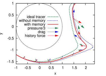
Figure 1: Trajectory of a single heavy particle ($R=0.4$ - sand in water, $S=0.01$) with respect to different dynamics: with memory (red), without memory (blue), and as an ideal tracer (green); initiated at $t_{0}=0.2$, $\boldsymbol{r}_{0}=\left(-1,\,-1.2\right)$ with vanishing slip velocity. The forces acting on the particle in the presence of memory are shown as arrows of different colors (red being the history force). The pressure term is presented with only a third of its magnitude.

First, we consider trajectories starting with the same initial condition, and compare different dynamics. Figure 1 shows the inertial trajectory of an aerosol with and without memory along with the trajectory of an ideal tracer (which follows the fluid velocity exactly). One immediately observes that the trajectories differ and that (at the beginning) the trajectory with memory is in-between the other two.

The acceleration of the particle can be decomposed into the three contributions on the right-hand side of (6). These terms, called the pressure term, the Stokes drag and the history force are plotted at subsequent time instants in figure 1. As the caption indicates, one third of the pressure term is given, for better visibility. We thus clearly see that the pressure term always dominates the other two, but the history force is of the same order as the Stokes drag. A comparison of the full trajectory with that obtained without the memory term (red and blue lines in figure 1, respectively) shows that the direction of separation (or approach) of theses trajectories coincides with the direction of the history force. For bubbles, similar findings have been reported in [39].

We also carried out simulations with equation of motion (17) valid in the weakly inertial limit. The results (not shown in figure 1) indicate a strong deviation from the true trajectory (red line), as strong as the deviation between this curve and any other curves in figure 1. This shows that a value as small as $S=0.01$ of the size parameter is not yet small enough to ensure the weakly inertial limit. At the same time, this is a sign indicating that dynamics (17) does not define a slow manifold [60, 61] for this $S$ (although it is expected to do so for sufficiently small $S$ values).

8 Ensemble and escape dynamics

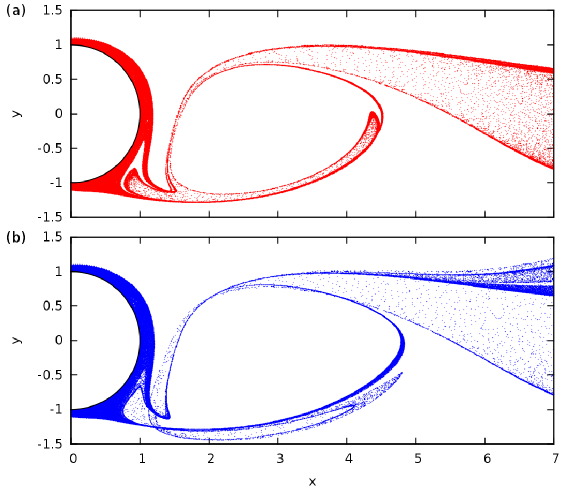
Figure 2: Dynamics of an ensemble of $N_{0}\approx 1.8\cdot 10^{6}$ aerosols ($R=0.4$ - sand in water, $S=0.01$) with (a) and without (b) memory starting in the domain $\left[-1,4\right]\times\left[-2,2\right]$ around the cylinder at $t_{0}=0.2$. The distribution of the particles is shown at time $t=0.94$.

Next, we turn to the dynamics of particle ensembles. A large number $N_{0}\approx 1.8\cdot 10^{6}$ of particles is distributed uniformly in the domain $\left[-1,4\right]\times\left[-2,2\right]$ around the cylinder at $t_{0}=0.2$. All particles are followed up to a certain time when we plot their position. The results for aerosols are shown in figure 2. The two distributions differ both in large- and small-scale structures. A characteristic feature of the case without the history force are caustics [4, 15], i.e., the intersection of different branches in the configuration space. This is due to the fact that what we see is a projection of the full pattern in the four-dimensional $(x,y,v_{x,}v_{y})$ phase space to a plane. Figure 2 shows that the frequency of occurrence of caustics seems to be lower with memory. We have found similar results for other values of $R$: $0.3$, $0.5$, $1.0$, $1.2$, $1.5$, $1.7$, $2.0$. This effect of the history force is even stronger for bubbles [39]. A quantity closely related to caustics is the collision rate. In accordance to the suppression of caustics, the history force has been found in [39] to lead to a reduction of the collision rate. A recent simulation [37] indicates a related phenomenon in turbulence: the history force is found to reduce preferential concentration (an effect which enhances collision rates).

In figure 2 a filamentary pattern can be seen both with and without the history force. This is in itself an indication for the chaoticity of the advection dynamics in both cases. Since the problem is dissipative, chaotic attractors might be present. Irrespective of their existence, chaos is always present in the form of transient chaos with an underlying chaotic set, a chaotic saddle [63, 64].

In the transient case all particles eventually escape downstream and the decay dynamics is best followed by monitoring the total number $N(t)$ of particles not yet escaped a given region up to time t. We distribute $N_{0}\approx 1.5\cdot 10^{6}$ particles uniformly in the domain $\left[0.6,4\right]\times\left[-2,2\right]$ outside the cylinder at initial time $t_{0}=0.2$. A particle is considered to have escaped if it crosses the line $x=5$ or it enters a circle of radius $r=1.014$ around the cylinder. The using of a circle larger in radius than the cylinder is motivated by excluding very slow (non-hyperbolic) decay characterizing the boundary layer, as done in [12, 59]. This definition of “escape” will be used throughout the paper, unless stated otherwise (as, e.g., in section 9). The number $N(t)$ of survivals is then determined as a function of time $t$. We find monotonous exponential decays with different characteristics for different cases.

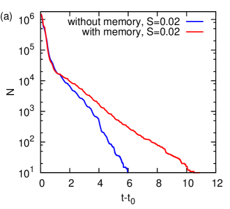
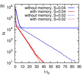
Figure 3: The number $N(t)$ of non-escaped particles for (a) $R=0.4$ - sand in water (b) $R=2.0$ - air bubble in water, with two different size parameters.

When the particles are heavier than the fluid (aerosols) typically all of them eventually escape; an example is shown in figure 3a. We see that the emptying process is slower with memory for aerosols. For bubbles attractors can appear for certain parameter values. An attractor presents itself as a plateau in $N(t)$, i.e., a fraction of all the particles never leaves the wake of the cylinder. See for example the case $S=0.04$ without memory in figure 3b; with memory the plateau, and thus the attractor, disappears. Here we see a profound change in the dynamics of inertial particles induced by the history force: the disappearance of attractors. When there are no attractors in the bubble case, the history force leads to a faster emptying of the wake. In the case of $S=0.02$ of figure 3b the time for a complete emptying roughly halves when memory is included. Note that the influence of the history force on the speed of the emptying process is opposite for aerosols and bubbles: memory slows down the emptying for aerosols and speeds it up for bubbles.

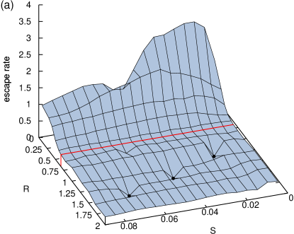
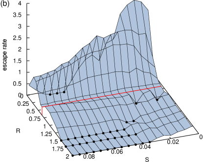
Figure 4: Escape rates on the parameter plane of size parameter and density ratio: $(S,R)$ with (a) and without (b) memory. The black dots mark parameters where an attractor is present. The $R$-values used as a grid of the plot are 0.1, 0.3, 0.4, 0.5, 0.6, $2/3$, 0.8, 1.0, 1.3, 1.5, 1.7, 2.0. The red line highlights the case of $R=2/3$, i.e., neutrally buoyant particles.

A quantitative measure characterizing the escape dynamics from the wake is the escape rate [63, 64]. It is the rate $\kappa$ of the exponential decay

$$N(t)\sim\exp(-\kappa t),$$ (21)

which sets in after an initial transient time, see figure 3. In the case of a plateau in $N(t)$ (due to the presence of an attractor) we set the escape rate formally to zero. Figure 4 shows the escape rate with and without memory as a function of the parameters $R$ and $S$. The red line marks the case of a neutrally buoyant particles ($R=2/3$), where the escape rate does not depend on $S$; indeed it is equal to the one of ideal tracers ($\kappa_{\mathrm{ideal}}=0.364$). We did not find any influence of memory on the behavior of neutrally buoyant particles. They behave as ideal tracers in this flow when the initial slip velocity is zero.

Attractors are quite ubiquitous without memory, see black dots in figure 4b. One even finds attractors in the aerosol range $R<2/3$. Since heavy particles are pushed outside of closed orbits due to the centrifugal force, and intend therefore to escape, attractors are expected to be atypical for aerosols. In special cases they were pointed out to exist [65, 66] and our results provide further examples of such cases. A striking effect of the history force is that it kills attractors at the parameters where they exist without memory. Only very few attractors (none for aerosols) are found with memory.

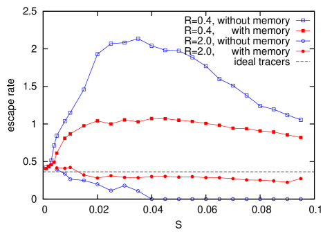
Figure 5: Escape rate as a function of $S$ with and without memory for $R=0.4$ and $R=2$.

The escape rates are typically closer to that of the passive (neurally buoyant) case with memory than without. In other words, the speed of the emptying process becomes less $R$-dependent. Figure 5 illustrates this tendency along two cuts (at $R=0.4$ and $R=2$). It is clear that the escape rates of aerosols (bubbles) become smaller (larger) due to memory, and that they are typically above (below) that of the passive case. There might be, however, exceptions as the bubble case with $S\leq 0.01$ illustrates where the escape rates slightly exceeds $\kappa_{\mathrm{ideal}}$. Note that the $S$-dependence is also weaker with memory. The escape process depends, thus, less on both parameters $R$ and $S$ when memory is taken into account.

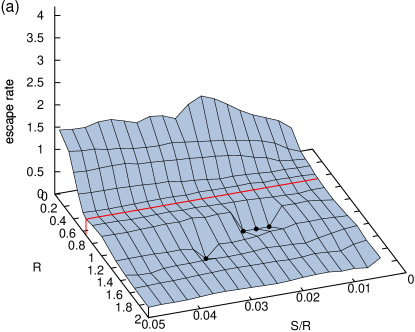
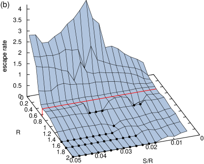
Figure 6: The same as figure 4 on the parameter plane $(St=S/R,R)$.

For completeness, we also present the escape rates on the plane of the Stokes number $St=S/R$ and the density ratio $R$, figure 6. Since in this representation the density plays a role along both axes, the graph of the escape rate is different but the general content remains the same.

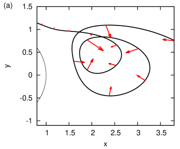
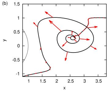
Figure 7: A comparison of the history force (red arrows) acting on an aerosol (a) and a bubble (b) along a spiraling trajectory in the wake. The parameters are $S=0.01$ and $t_{0}=0$ in both cases and $R=0.4$, $\boldsymbol{r}_{0}=\left(-0.5,1.2\right)$ for the aerosol and $R=2$, $\boldsymbol{r}_{0}=\left(-0.5,-1.14\right)$ for the bubble. The scale of the arrows for the bubble case is 10 time larger, i.e., in this case the history force is much stronger (this is also true for the the other forces). Note that the history force counteracts the centrifugal force in both cases.

An important effect of the history force can be observed when studying particles moving along general curved trajectories: the history force is found to counteract the centrifugal force. Heavy particles are pushed outwards of vortex centers by the centrifugal force. Memory is seen to generate a dissipative effect which provides a force pointing towards the center of a vortex, as illustrated by figure 7a. For bubbles the effect is opposite, i.e., the history force points outwards the center of a vortex; it counteracts the (anti)centrifugal force which pushes bubbles inside of vortices. This behavior has been also found in [67] for the analytically treatable case of a single vortex with the flow field $\boldsymbol{u}(\boldsymbol{r})=\left|\boldsymbol{r}\right|\boldsymbol{e}_{\varphi}$. The effect visualized in figure 7 provides a qualitative explanation for the decrease (increase) of the escape rate for heavy (light) inertial particles in the presence of memory.

We can summarize that, in general, the history force tends to weaken the difference between particle and fluid and “pushes” the dynamics towards that of the ideal case.

9 Residence time and non-hyperbolic behavior

Figure 8: Residence times with (a) and without (b) memory for $R=2.0$, $S=0.02$, $t_{0}=0$. The escape condition is $x>5$ ($r<1.014$ is not counted here as an escape). The logarithm ($\log_{10}$) of the residence time is color-coded.

A further characterization of the escape dynamics is via the residence time distribution. To any initial position in the flow, we determine the time the particle takes to escape and indicate this time via color-coding. The trajectories are integrated up to a maximum of $100$ time units, thus the largest residence time found is $100$. In this section we do not cut out the circle of radius 1.014 along the cylinder surface (unlike in the previous sections), and the escape condition is simply $x>5$, in order to also see the effect of the stickiness of the wall. Figure 8 shows the result with and without memory for bubbles. Very long lifetimes, longer than $100$ time units, would indicate basins of attraction of an attractor. In this case no attractors exist and lifetimes on the order of 100 mark slowly moving trajectories which will spend a long time in the boundary layer close to the cylinder surface. We see clearly that the area of initial conditions with long lifetimes (redish colors) is much lower with memory than without. Thus the surface of the cylinder seems to be less sticky when memory is included. Furthermore the structure of the residence time distribution shows a clear dependence on the presence of memory also away from the cylinder surface, e.g. in the region $\left[1.5,3.5\right]\times\left[-1.5,0\right]$ where a vortical pattern is present with memory.

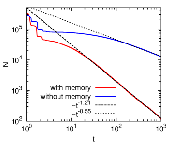
Figure 9: Long time, non-hyperbolic regime of the escape dynamics for bubbles. Parameters are the same as in figure 8.

In dynamical system terms, the sticky surface of the cylinder leads to a non-hyperbolic behavior marked by a long-term power law decay of the number of survivors. For trajectory ensembles containing initial points close to the surface one finds that the number N(t) of non-escaped particles up to time t behaves for $t\gg 1$ as

$$N(t)\sim t^{-\sigma},$$ (22)

where $\sigma$ is the exponent of the non-hyperbolic decay [68]. The number of survivors in the range of 100 and 1000 time units exhibits clear straight lines on a log-log plot in both cases, as can be seen in figure 9. The slopes are, however, different. We have found a change from $\sigma=0.55$ to $\sigma=1.21$ when memory is included. (For ideal tracers $\sigma=2$ [52].) For bubbles, memory effects lead thus to a faster decay (to an increased decay exponent), weaken non-hyperbolicity, but do not destroy the power-law behavior. For aerosols, the effect of the cylinder wall appears to be much weaker both with and without memory, and we don’t find any change of the non-hyperbolic decay exponent.

10 Statistics of forces, slip velocity and acceleration

In section 7 we briefly discussed the forces acting along a sample trajectory. To be able to make more general statements we now turn to the statistics of these forces. The statistics presented in this section are obtained by averaging over an ensemble of $N_{0}\approx 1.8\cdot 10^{6}$ aerosols $(R=0.4,S=0.01)$, started in the domain $\left[-1,4\right]\times\left[-2,2\right]$ at $t_{0}=0.2$; we sampled over all time instants at which a particle has not yet escaped the wake of the cylinder.

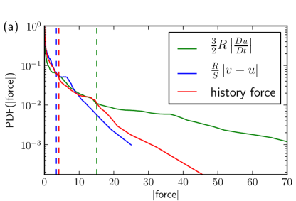
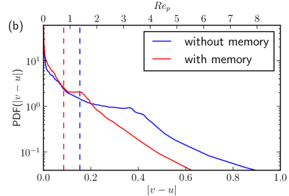
Figure 10: (a) The PDF of the magnitude of the forces on the rhs of (6), with memory.
(b) PDF of the magnitude of the dimensionless slip velocity $\left|\boldsymbol{v}-\boldsymbol{u}\right|$ with and without memory. The x-axis on the top shows the particle Reynolds number $Re_{p}$, which is proportional to the slip velocity (see (20)). Vertical lines indicate the position of the corresponding averages. The parameters are $R=0.4$, $S=0.01$. The ensemble consists of $N_{0}\approx 1.8\cdot 10^{6}$ particles initiated in the domain $\left[-1,4\right]\times\left[-2,2\right]$ around the cylinder at $t_{0}=0.2$; a particle is part of the ensemble only until it escapes.

Figure 10a shows the probability density function (PDF) of the magnitude of the three forces appearing on the right-hand side of (6). Let us first compare the averages of the different forces, shown as vertical lines in figure 10a. We see that our observations from section 7 based on a single example trajectory also hold true for the averages: the pressure term is the dominant one and the history force (red curve in figure 10a) is of similar magnitude as the Stokes drag. Looking at the tails of the PDFs we observe that the pressure term has a particularly large amount of extreme events and the history force has a slightly longer tail (more extreme events) then the Stokes drag.

The ratio of the averages of the history force and of the Stokes drag in figure 10a is $F_{h}/F_{d}=1.21$. In view of this finding, (12), and the fact that $\sqrt{S}=0.1$, we conclude that parameter $\alpha$ is $\sqrt{2/9}\times 12.1=5.7$ in this setting. The observation that the $\alpha$ value is not close to $1$ shows that the importance of the history force cannot be estimated solely by $\sqrt{S}$; parameter $\alpha$ is also relevant. If we neglected $\alpha$, we would underestimate the history force by a considerable amount.

In order to be a useful parameter for estimating the importance of the history force, $\alpha$ should be independent of $S$. Indeed, for $R=0.4$ we find $\alpha\in[4.7,6.0]$ and for $R=2.0$ $\alpha\in[7.2,7.7]$ when $S$ is varied between $0.05$ and $0.005$. For the purpose of rough estimates we can thus consider $\alpha$ constant, with a value around $5$ (in this flow).

Figure 10b shows the PDF of the magnitude of the slip velocity $\left|\boldsymbol{v}-\boldsymbol{u}\right|$. It is important to see that the average is much below $1$ in both cases, indicating that the deviation between the particle and the flow velocity is typically much smaller than the flow velocity itself. Furthermore, the average dimensionless slip velocity $0.153$ of the memoryless case is reduced to $0.085$ (to ca. $55\%$) when the history force is included. Thus, particles with memory follow the fluid more closely. In harmony with this, the tail of the slip velocity PDF becomes shorter with memory, i.e., there are less strong “detachments” from the fluid flow. We find the same tendency for bubbles albeit somewhat weaker, e.g. for $R=2$, $S=0.01$ the slip velocity is reduced to $85\%$ by memory. All this illustrates that the history force provides an important viscous contribution so that the resultant of it and the drag ensures a faster relaxation towards the flow velocity than the drag alone.

Equation (20) shows that the slip-velocity is proportional to the instantaneous $Re_{p}$. Accordingly, the top axis of figure 10b displays $Re_{p}$. Its average for particles with (without) memory is found to be $0.76$ ($1.36$). The assumption that the particle Reynolds number remains of order unity or smaller is thus found to be fulfilled on average, with a somewhat sharper bound with memory.

The statistics of the acceleration of particles (not shown) is also consistent with the picture above. Ideal tracers have the highest average acceleration and the most extreme events (the longest tail in the PDF). The case without memory exhibits the lowest accelerations, and the inclusion of memory increases the average acceleration, as well as, the probability of extreme events. Thus we see again that the statistics come closer to that of the ideal case when memory is included.

11 Periodic attractors

Let us now turn to a parameter set where attractors are present both with and without memory: $w=24$ (instead of $192/\pi$), where $w$ describes the strength of the vortices behind the cylinder, and $R=1.5$, $S=0.03$. The residence times are depicted in figure 11. Their structure changes significantly when memory is taken into account, as we have already seen in section 9. Here we included again the circle of radius $1.014$ as an escape condition to exclude the non-hyperbolic decay. Thus residence times of 100 (the maximum integration time) show initial conditions leading to an attractor. In the presence of memory, the basin of attraction (marked by red) becomes significantly smaller; its area is reduced by a factor of about $2.5$. Thus, we can say that memory makes the attractor less attractive in this case. We note, that for this choice of $w$ there are also trajectories of ideal tracers which never leave the wake. Tiny integrable regions exist which appear as red dots in figure 11c. Comparing the residence time plots we see again that the case with memory comes closer to that of ideal tracers.

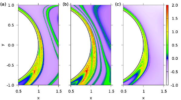
Figure 11: Residence times for bubbles with (a) and without memory (b), and for ideal tracers (c). The parameters are $R=1.5$, $S=0.03$, $t_{0}=0.3$, $w=24$. The logarithm ($\log_{10}$) of the residence time is color-coded.

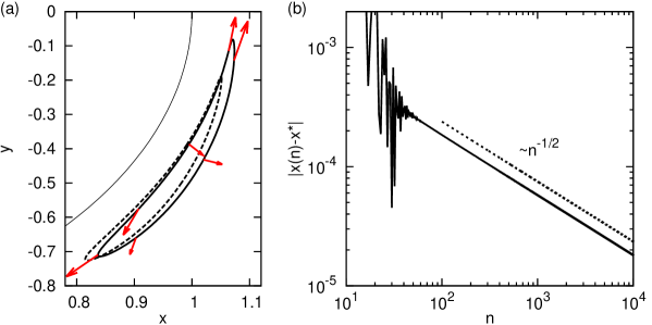
Figure 12: (a) Attractors with and without memory (solid and dashed line, respectively) traced out by approaching trajectories after $10^{4}$ time units (the parameters are $R=1.5$, $S=0.03$, $t_{0}=0.3$, $w=24$.). The arrows represent the history force. (b) Distance between an approaching trajectory with memory and the corresponding asymptotic attractor at integer times.

It is worth comparing the attractors with and without memory. Both attracting objects appear to be periodic orbits of period-1 (i.e., with the same period as the vortex shedding period), and are of similar form, as figure 12a shows. Note that the history force does not vanish on the attractor with memory. A basic difference between the two cases is that the attractor of the memoryless case is stationary by the time the plot is made, but the cycle-looking object seen in the presence of memory keeps changing very slowly in time. It is thus a ’quasi-attractor’ only. A real attractor is expected to be reached (even in a numerical sense) after a very long time only.

We examine the convergence of the trajectory to the attractor through the quantity $\left|x(n)-x^{*}\right|$, where $x(n)$ and $x^{*}$ is the $x$-coordinate of an approaching trajectory after $n$ time units and of the asymptotic attractor ($x^{*}=\lim_{n\rightarrow\infty}x(n)$), respectively. This corresponds to taking snapshots at integer multiples $n$ of the period, i.e., a stroboscopic map. The time dependence of this quantity is shown in figure 12b for the case with memory. The convergence follows a $t^{-1/2}$ law, where the exponent is obviously related to the power law behavior of the kernel of the history force (5). The algebraic convergence is in strong contrast to normal dynamical systems where the convergence is exponential. This means that with memory the convergence is very slow and that there is no characteristic time scale characterizing this convergence.

The fact that a periodic attractor is possible with memory can be explained by the observation that after a very long time the memory of the approach to the attractor decays away, and the dynamics remembers only what has been in the close vicinity of the attractor, on a loop like the continuous line in figure 12a, and a convergence becomes thus possible.

12 Interpretation in terms of snapshot attractors

Using this classical single trajectory picture, one concludes that the attractor can be reached after a very long period of time only. There is, however, an alternative view, that of particle ensembles, also available. In autonomous systems the two views are equivalent, which is not so obvious in non-autonomous problems, like ours (see (11)). In this class, one can then define a snapshot attractor as an object which attracts all the trajectories initialized in the infinitely remote past within a basin of attraction [69, 70]. It can be obtained by monitoring an ensemble of particle trajectories all subject to the same non-autonomous equation of motion. After a characteristic dissipative time, the ensemble traces out a snapshot attractor. This attractor might, however, move continuously in time.

In the dynamical systems community, the concept has been known for many years [69]. The idea proved to be particularly well suited for understanding the advection of passive particles in random flows [71, 72, 73], and explains experimental findings [74]. More recently, snapshot attractors have turned out to be promising tools to describe the variability of climate dynamics in a novel way [70, 75, 76, 77, 78]. In these settings the non-autonomous driving is typically a random noise or a sustained chaotic process. The snapshot attractor is then ever changing, and appears to be a fractal object whose shape is evolving in time. In cases with an eventually vanishing driving, the snapshot attractor might have a time-dependence that ceases asymptotically.

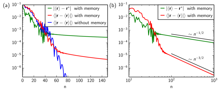
Figure 13: Convergence of an ensembles of 100 particles towards a fixed point attractor on the stroboscopic map with memory and without memory. The ensemble consists of 100 randomly chosen initial conditions from the basin of attraction in the region $[0.5,1.5]\times[-1,1]$. The green curve represents the distance of the center of mass from the true, asymptotic attractor $\boldsymbol{r}^{*}$ (an analog of figure 12b). The other curves represent the average radius of the ensemble (the red one with, the blue one without memory). Panels (a) and (b) are log-lin and log-log representations and focus on the short and long time approach, respectively. The parameters are $R=1.5$, $S=0.03$, $t_{0}=0.3$, $w=24$.

For our problem of chaotic advection with memory, where a slow convergence towards a traditional periodic attractor takes place, one can assume that close to this attractor the effect of the history force for neighboring members of the particle ensemble can locally be considered as a non-autonomous perturbation superimposed on the usual inertial particle dynamics. An ensemble of particles might then converge to a snapshot attractor, a fixed point on the stroboscopic map, after some time. This snapshot fixed point attractor is then slowly shifted towards the asymptotic traditional attractor. Here a separation of time scales is expected to occur since the convergence to the snapshot attractor is a usual dissipative effect, and hence this decay should be exponential, whereas the slow shift is due mainly to the diffusive kernel, and follows thus a power law.

To verify this we choose an ensemble of $100$ particles approaching the periodic attractor, and compute the center of mass $\left\langle\boldsymbol{r}(n)\right\rangle$ (i.e., the average of the spatial location vector over the ensemble) and the radius of the ensemble $\left\langle\left|\boldsymbol{r}(n)-\left\langle\boldsymbol{r}(n)\right\rangle\right|\right\rangle$ at integer times $n$. The center of mass represents the time-dependent position of the snapshot attractor whereas the radius is a measure of convergence to the snapshot attractor. The center of mass is found to exhibit the same power-law behavior, of power $-1/2$, as $x(n)$. However, we observe that the radius of the ensemble has an initial roughly exponential decay, see figure 13a, which crosses over to an algebraic decay of power $-3/2$. Thus we conclude that the point-like object formed after about 70 time units is a snapshot fixed point attractor emerging as an effect of memory.

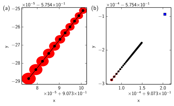
Figure 14: Positions of an ensemble of 100 particles (the same as in figure 13) approaching a fixed point attractor on the stroboscopic map. Black dots and red circles around them represent the center of mass and the radius, respectively, of the ensemble. The parameters are the same as in figure 13. (a) The positions of the ensemble at time instants $200$, $210$, …, $300$. (b) The positions of the ensemble at time instants $200$, $220$, …, $1000$. The circles indicating the radius are hardly visible at this scale. The asymptotic fixed point attractor is marked by a square. Note the largely magnified scales in both panels.

To deepen this picture, we plot in figure 14 the center of mass and the radius of the ensemble in the plane of the fluid at integer times. Figure 14a shows time instants between $n=200$ and $300$, whereas figure 14b covers the range $[200,1000]$. The scale is strongly magnified but the plot clearly indicates that the fixpoint snapshot attractor slowly moves. Even after $1000$ time units it is still away from the limiting location. The latter is determined from a self-consistent fit to the algebraic decay process of the center of mass.

The evolution can thus be split into a short-time and a long-time regime. In the first one, up to about $70$ time units, a convergence to a snapshot attractor takes place. In the second one (for $n>70$) a snapshot attractor is reached but it is shifted slowly towards an asymptotic fixed point, the traditional attractor.

13 Chaotic attractors

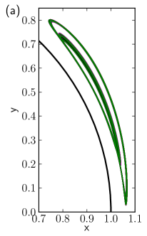
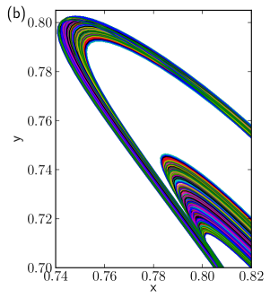
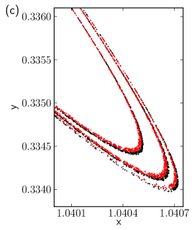
Figure 15: Chaotic attractor with memory. (a) Positions of an ensemble of 100 trajectories (marked by different colors) traced out in the time interval $t\in[990,1000]$; (b) A magnification. The ensemble consists of 100 randomly chosen initial conditions from the basin of attraction in the region $[0.5,1.5]\times[-1,1]$. The parameters are $R=1.47$, $S=0.049$, $t_{0}=0.3$, $w=31.2$. (c) Positions on a stroboscopic map (on a magnified scale). The red dots correspond to the attractor points at $n\in[600,800]$ and the black dots to those at $n\in[800,1000]$. We observe a slow motion of the attractor obtained in the ensemble picture.

Chaotic attractors with memory are very rare in the parameter range investigated and we had to perform an extended parameter-scan to find one. In figure 15a we see an ensemble of 100 trajectories (in continuous time) tracing out this chaotic attractor with memory. A magnification, figure 15b, indicates clear fractal properties. The Lyapunov exponent of this attractor is $\lambda=0.18\pm 0.01$. It is positive, which shows that the attractor is chaotic indeed. Details of how the largest Lyapunov exponent can be determined in such a system with long memory is given in A. We note that at this parameter values (given in the caption to figure 15) the attractor without memory is not chaotic.

Figure 15c exhibits the stroboscopic picture of the chaotic attractor with memory. It shows a magnification in two different time intervals: $t\in[600,800]$ and $t\in[800,1000]$. A shift on the order of $10^{-4}$ units can be observed, a clear manifestation of the fact that this chaotic attractor is slowly drifting, similar to the fixed point snapshot attractor discussed in the previous section.

14 Chaotic saddles

In contrast to permanent chaos, transient chaos is ubiquitous in the problem as the typical form of chaos in this open flow. Chaotic transients are found at any parameter, irrespective of the existence of attractors. The degree of chaos can thus best be compared by comparing the underlying chaotic saddles which exist both for ideal tracers and inertial particles with or without memory.

To construct the saddle, we consider particles with long residence times, longer than $15$ time units. The idea is that these particles come close to the saddle and then leave the wake. The longer the particle stays in the wake, the closer it comes to the saddle. One might suppose that at half of their residence time ($t=7$) the particles are closest to the saddle and thus their positions at this time trace out the saddle. This is supported by the observation that this set of points at $t=7$ is only marginally different from those at $t=6$ and $t=8$, i.e., the set is (approximately) invariant. Figure 16a shows the saddle constructed by this method for three different advective dynamics. The initial positions of particles which stay long in the flow and thus come close to the saddle trace out the stable manifold of the chaotic saddle, and are plotted in figure 16b.

We see that the saddle and its stable manifold change considerably when the history force is taken into account. It is interesting to note that the saddle and its stable manifold differ much more from those of ideal tracers than from the memoryless case. This illustrates that the general rule according to which the presence of memory makes the dynamics to be similar to that of ideal tracers is not true in all possible aspects.

To further characterize the saddle and the corresponding dynamics we calculated the Lyapunov exponent, as described in A. The Lyapunov exponent with the history force is found to be $\lambda=0.91\pm 0.02$. This is larger then without memory, when $\lambda=0.79\pm 0.02$, and is close to that of ideal tracers for which $\lambda=0.92\pm 0.02$. Thus particles with memory are dynamically more unstable, and their measure of instability is closer to that of ideal tracers.

Figure 16: (a) The chaotic saddle for inertial particles with memory (red), without memory (blue), and for ideal tracers (green). The saddle without memory and the one for ideal tracers are shifted horizontally by 0.1 and 0.2, respectively, for better visibility. (b) The stable manifolds of the corresponding saddles. The parameters are $R=2.0$, $S=0.02$, $t_{0}=0$, the same as in figure 8.

15 Summary and discussion

In summary, memory effects can have a very significant influence on inertial particles. In the presence of the history force, compared to the memoryless inertial case, we find:

• a rare appearance of attractors, especially of chaotic ones,

• a less frequent appearance of caustics,

• a decrease of the centrifugal effect,

• a slower (faster) escape for aerosols (bubbles),

• a weaker effect of the cylinder wall,

• a stronger dynamical instability on chaotic sets,

• a very slow, algebraic convergence to attractors (when defined in the usual single trajectory picture),

• a tendency of the particles to follow the flow more closely.

As a trend, the dynamics become more similar to that of ideal tracers when the history force is included (although exceptions can also be found, see, e.g., figure 16).

In one principal aspect the dynamics basically differs, however, from both the usual inertial and the passive tracer dynamics. Due to memory, the problem is strictly speaking high-dimensional, and methods known from low-dimensional dynamical systems are not necessarily applicable. For understanding the slow convergence towards periodic attractors, the concept of snapshot attractors appears to be useful. More generally, we assume that the snapshot interpretation, i.e., considering the instantaneous position of an ensemble of trajectories started in the remote past, is applicable for any kind of asymptotic sets (chaotic attractors, chaotic saddles) in advection with memory effects. In this new picture, an exponential convergence to a snapshot-like attractor is expected to show up, which is then slowly changing afterwards.

Let us come back to estimation (12) of the importance of the history force. A question of relevance is whether one can determine a typical value for $\alpha$ in general. For the following argument we assume the time to be dimensional again. Imagine a signal $f(t)$ which varies on the time scale $\tau$. Then we can estimate the magnitude of the derivative $\frac{\mathrm{d}f}{\mathrm{d}t}$ by $|f|/\tau$. Extrapolating this reasoning to fractional derivatives, we expect the magnitude of $\left(\frac{\mathrm{d}}{\mathrm{d}t}\right)^{1/2}f$ to be roughly $\sqrt{1/\tau}|f|$. Thus, setting $f=\boldsymbol{v}-\boldsymbol{u}$ in (13) we obtain

$$\alpha\equiv\frac{\sqrt{T}\left(\frac{\mathrm{d}}{\mathrm{d}t}\right)^{1/2}(\boldsymbol{v}-\boldsymbol{u})}{\boldsymbol{v}-\boldsymbol{u}}\approx\sqrt{\frac{T}{\tau}}.$$ (23)

In our flow the time unit $T$ is chosen, traditionally, as the shedding period of the vortices. As particles “live” on the small scales, $\tau$ should be the smallest time scale of the flow. In the von Kármán problem there are two characteristic times: the shedding period $T$ and the convective time scale $L/U$. The later is the smaller one and can be considered to be the time a particle needs for going around a vortex. We thus take $\tau=L/U$ in (23) and find, in view of (15), that

$$\alpha\approx\sqrt{\frac{TU}{L}}=Sl^{-1/2}.$$ (24)

Using the value $Sl=1/14$ we obtain $\alpha\approx 3.7$, which is quite close to the measured range $4.7\leq\alpha\leq 7.7$.

The reason $\alpha$ turns out to depend on $Sl$ is that we have used the shedding period $T$ to nondimensionalize the equation of motion, rather than the smaller time scale $\tau=L/U$. Thus we conclude, a posteriori, that a more natural choice is to use the convective time scale from the very beginning. Denoting the corresponding quantities in this time unit with a prime, we obtain $\alpha^{\prime}\approx 1$ and

$$\frac{F_{h}}{F_{d}}\approx\sqrt{\frac{9}{2}S^{\prime}}$$ (25)

with a modified size parameter

$$S^{\prime}=\frac{2}{9}\frac{a^{2}/\nu}{\tau}.$$ (26)

We thus see that for the size parameter (and the Stokes number) — a Lagrangian quantity — the use of the smallest time scale, the convective time scale $L/U$, is natural. It leads to simpler expressions, in contrast to using the shedding period $T$ which is the usual choice in the Eulerian characterization of this flow.

Let us come to a more general statement about other flows. From (25) and (26) we obtain the rather simple formula

$$\frac{F_{h}}{F_{d}}\approx\frac{a}{\sqrt{\tau\nu}}$$ (27)

for the estimation of the history force relative to the Stokes drag. We expect this to be a good estimation also in other flows as long as the time scale $\tau$ is chosen to be the smallest time scale of the flow. This choice becomes particularly important in multi-scale flows. Note also that the convective time scale need not necessarily be the smallest time scale in other flows. However, when this is fulfilled and when the flow is smooth with only one characteristic length scale $L$ (like the flow examined in this paper) we get

$$\frac{F_{h}}{F_{d}}\approx\frac{a}{L}\sqrt{Re}.$$ (28)

Let us finally remark on the possible role of memory effects in turbulent flows. In turbulence, the time scale $\tau$ should be the Kolmogorov time scale $\tau_{K}$ [79]. Using $\nu\tau_{K}=\eta^{2}$ in (27), where $\eta$ is the Kolmogorov length, we obtain

$$\frac{F_{h}}{F_{d}}\approx\frac{a}{\eta}$$ (29)

as an estimate for the importance of the history force. We thus expect memory effects to be negligible for $a<10^{-2}\eta$. For $a$ around $0.1\eta$ the history force should be around $10\%$ of the Stokes drag and is thus expected to be clearly observable. However, when $a$ is close to $\eta$, the history force can be as important as the Stokes drag indicating strong memory effects even in turbulent flows. (Note that in the latter case Faxén corrections might also be important.)

16 Acknowledgments

Useful discussions with J.-R. Angilella, T. Bohr, I. Benczik, B. Eckhardt, M. Farazmand, U.  Feudel, K. Guseva, G. Haller, E. Ott, A. Pumir and M. Wilczek are acknowledged. The project is supported by the grant OTKA NK100296. We acknowledge support by the Alexander von Humboldt Foundation, the Studienstiftung des deutschen Volkes, the Deutsche Forschungsgemeinschaft, and the Open Access Publication Fund of University of Muenster.

Appendix A Lyapunov exponents in the presence of the history force

Lyapunov exponents characterize the evolution of infinitesimal perturbations in time. For the full Maxey-Riley equation (6) the equations governing this evolution are

$$\frac{1}{R}\frac{\mathrm{d}}{\mathrm{d}t}\delta\boldsymbol{v} = \frac{3}{2}\delta\boldsymbol{r}\cdot\nabla\frac{\mathrm{D}\boldsymbol{u}}{\mathrm{D}t}-\frac{1}{S}\delta\boldsymbol{v}-\frac{1}{S}\delta\boldsymbol{r}\cdot\nabla\boldsymbol{u}$$

$$-\sqrt{\frac{9}{2\pi}\frac{1}{S}}\frac{\mathrm{d}}{\mathrm{d}t}\int_{t_{0}}^{t}\frac{1}{\sqrt{t-\tau}}\left(\delta\boldsymbol{v}-\delta\boldsymbol{r}\cdot\nabla\boldsymbol{u}\right)\,\mathrm{d}\tau,$$

$$\frac{\mathrm{d}}{\mathrm{d}t}\delta\boldsymbol{r} = \delta\boldsymbol{v}.$$

Here $\delta\boldsymbol{q}(t)\equiv(\delta\boldsymbol{r}(t),\delta\boldsymbol{v}(t))$ is an infinitesimal perturbation along a given trajectory $\boldsymbol{q}(t)\equiv\left(\boldsymbol{r}(t),\boldsymbol{v}(t)\right)$. Equation (A) is an evolution equation with memory. The (largest) Lyapunov exponent is then defined as

$$\lambda=\lim_{t\rightarrow\infty}\frac{1}{t-t_{0}}\ln\frac{\left|\delta\boldsymbol{q}(t)\right|}{\left|\delta\boldsymbol{q}(t_{0})\right|}.$$ (31)

We assume that this quantity is the same for (almost) all trajectories of a chaotic set, as in standard dynamical systems theory [63].

One way to compute $\lambda$ is to numerically integrate (A). However, often it is more convenient to obtain the evolution of perturbations directly from pairs of particles starting close to each other. To a given trajectory $\boldsymbol{q}(t)$ one computes a perturbed trajectory $\boldsymbol{q}^{\prime}(t)$ starting from a perturbed initial condition

$$\boldsymbol{q}^{\prime}(t_{0})=\boldsymbol{q}(t_{0})+\Delta\boldsymbol{q}_{0},$$ (32)

where $\Delta\boldsymbol{q}_{0}$ is a small but finite perturbation, and obtains the Lyapunov exponent from

$$\lambda=\lim_{t\rightarrow\infty}\frac{1}{t-t_{0}}\ln\frac{\left|\Delta\boldsymbol{q}(t)\right|}{\left|\Delta\boldsymbol{q}_{0}\right|}$$ (33)

with

$$\Delta\boldsymbol{q}(t)=\boldsymbol{q}^{\prime}(t)-\boldsymbol{q}(t).$$ (34)

For this to be close to the original definition of $\lambda$ (31) one has to make sure that $\Delta\boldsymbol{q}(t)$ is small for all $t$, i.e., $\Delta\boldsymbol{q}(t)$ evolves according to a linear evolution equation. A naive method would be to choose $\Delta\boldsymbol{q}_{0}$ so small that for a given integration time $t_{\mathrm{end}}$ one can be sure that $\Delta\boldsymbol{q}(t)$ remains small. However $\Delta\boldsymbol{q}_{0}$ can not be too small due finite numerical precision, because then $\boldsymbol{q}^{\prime}$ would be numerically indistinguishable from $\boldsymbol{q}$.

The approach we use is to start with a small but not too small perturbation ($\left|\Delta\boldsymbol{q}_{0}\right|=\Delta q_{min}$) and adjust $\boldsymbol{q}^{\prime}$ by rescaling $\Delta\boldsymbol{q}$ when $\left|\Delta\boldsymbol{q}(t)\right|$ becomes larger than a given threshold $\Delta q_{max}$. This way we make sure that $\Delta\boldsymbol{q}$ remains small. The procedure is as follows:

1. integrate $\boldsymbol{q}^{\prime}$ up to a time $\tilde{t}$ when $\left|\Delta\boldsymbol{q}\right|=\Delta q_{max}$,

2. set $\boldsymbol{q}^{\prime}(t):=\boldsymbol{q}(t)+\Delta\boldsymbol{q}(t)\frac{\Delta q_{min}}{\Delta q_{max}}$ for $t_{0}\leq t\leq\tilde{t}$, and proceed with the integration for $\tilde{t}<t$,

3. repeat step 1 and 2 until the desired integration time $t_{\mathrm{end}}$ is reached.

This rescaling makes sense because $\boldsymbol{q}^{\prime}$ and $\boldsymbol{q}$ are rather close and thus $\Delta\boldsymbol{q}$ evolves according to the linear equation (A). Therefore, at any iteration of the above procedure, $\Delta\boldsymbol{q}(t)\Delta q_{min}/\Delta q_{max}$ is an (approximate) solution of (A) and $\boldsymbol{q}^{\prime}(t):=\boldsymbol{q}(t)+\Delta\boldsymbol{q}(t)\Delta q_{min}/\Delta q_{max}$ is a valid perturbed trajectory.

The key idea is that when the upper bound $\Delta q_{max}$ is reached, we just choose another solution $\boldsymbol{q}^{\prime}$ which starts at a smaller initial perturbation $\Delta\boldsymbol{q}_{0}$; the new perturbation is smaller but proportional to the previous one. As $\Delta\boldsymbol{q}$ evolves according to a linear equation, we can efficiently obtain the new solution by simple rescaling. Because we rescale the previous solution and continue with the integration only for $\tilde{t}<t$, we avoid computations with too small $\Delta\boldsymbol{q}$.

With the history force it is important to adjust $\boldsymbol{q}^{\prime}$ for the whole past $t_{0}\leq t\leq\tilde{t}$ because the evolution depends on the whole past. Without memory one would only need to adjust $\boldsymbol{q}(\tilde{t})$, which leads to a standard method of computing the Lyapunov exponent [81, 63].

When a perturbation trajectory $\Delta\boldsymbol{q}$ has been computed up to $t=t_{\mathrm{end}}$, we obtain the Lyapunov exponent from

$$\lambda\approx\frac{1}{t_{\mathrm{end}}-t_{0}}\ln\frac{\left|\Delta\boldsymbol{q}(t_{\mathrm{end}})\right|}{\left|\Delta\boldsymbol{q}_{0}\right|},$$ (35)

where $t_{\mathrm{end}}$ is a large integration time.

In section 14 we are dealing with transient chaos. Therefore the length of the trajectories is limited and it is difficult to accurately compute the Lyapunov exponent from a single trajectory. Therefore we use a preselected ensemble of trajectories which stay close to the saddle for a sufficiently long time, as in other cases of transient chaos [68]. Equation (35) defines the Lyapunov exponent as the slope of the function $\ln\left|\Delta\boldsymbol{q}(t)\right|$, computed using its values at $t=t_{0}$ and $t=t_{\mathrm{end}}$. We extend this idea to an ensemble by computing the average

$$d(t)=\left\langle\ln\frac{\left|\Delta\boldsymbol{q}(t)\right|}{\left|\Delta\boldsymbol{q}_{0}\right|}\right\rangle$$ (36)

and making a linear fit to $d(t)$ to obtain the slope which is the Lyapunov exponent $\lambda$. In section 14 we choose trajectories which stay in the wake for at least 15 time units and make a linear fit in the range $t\in[5,15]$.

References

References

- [1] Magnaudet J and Eames I 2000 Ann. Rev. Fluid Mech. 32 659–708
- [2] Toschi F and Bodenschatz E 2009 Annu. Rev. Fluid Mech. 41 375–404
- [3] Cartwright J H, Feudel U, Károlyi G, de Moura A, Piro O and Tél T 2010 Dynamics of finite-size particles in chaotic fluid flows Nonlinear Dynamics and Chaos: Advances and Perspectives (Springer) pp 51–87
- [4] Falkovich G, Fouxon A and Stepanov M 2002 Nature 419 151–154
- [5] Grabowski W W and Wang L P 2013 Annual Review of Fluid Mechanics 45 293–324
- [6] Bracco A, Chavanis P H, Provenzale A and Spiegel E A 1999 Physics of Fluids 11 2280–2287
- [7] Nishikawa T, Toroczkai Z and Grebogi C 2001 Phys. Rev. Lett. 87(3) 038301
- [8] Zahnow J C, Vilela R D, Feudel U and Tél T 2009 Phys. Rev. E 80(2) 026311
- [9] Zahnow J C, Maerz J and Feudel U 2011 Physica D 240 882 – 893
- [10] Ouellette N T, O’Malley P J J and Gollub J P 2008 Phys. Rev. Lett. 101(17) 174504
- [11] Sapsis T, Ouellette N, Gollub J and Haller G 2011 Physics of Fluids 23 093304
- [12] Benczik I, Toroczkai Z and Tél T 2002 Phys. Rev. Lett. 89 164501
- [13] Tang W, Haller G, Baik J J and Ryu Y H 2009 Phys. Fluids 21 043302 (pages 7)
- [14] Bec J, Biferale L, Cencini M, Lanotte A, Musacchio S and Toschi F 2007 Phys. Rev. Lett. 98 084502
- [15] Wilkinson M and Mehlig B 2005 Europhys. Lett. 71 186
- [16] Maxey M R and Riley J J 1983 Phys. Fluids 26 883–889
- [17] Gatignol R 1983 J. Mec. Theor. Appl 1 143–160
- [18] Auton T R, Hunt J C R and Prud’Homme M 1988 J. Fluid Mech. 197 241–257
- [19] Landau L D and Lifshitz E M 1987 Fluid Mechanics, Vol. 6 Course of Theoretical Physics (Pergamon Press)
- [20] Michaelides E E 2006 Particles, Bubbles and Drops: Their Motion, Heat And Mass Transfer (World Scientific, Singapore)
- [21] Druzhinin O A and Ostrovsky L 1994 Physica D 76 34 – 43
- [22] Mordant N and Pinton J 2000 Eur. Phys. J. B 18 343–352
- [23] Abbad M and Souhar M 2004 Physics of Fluids 16 3808
- [24] Hill R J 2005 Physics of Fluids 17 037103
- [25] Angilella J R 2007 Physics of Fluids 19 073302
- [26] Toegel R, Luther S and Lohse D 2006 Phys. Rev. Lett. 96 114301
- [27] Garbin V, Dollet B, Overvelde M, Cojoc D, Di Fabrizio E, van Wijngaarden L, Prosperetti A, de Jong N, Lohse D and Versluis M 2009 Physics of Fluids 21 092003
- [28] Kheifets S, Simha A, Melin K, Li T and Raizen M G 2014 Science 343 1493–1496
- [29] Yannacopoulus Y, Rowlands G and King G 1997 Phys. Rev. E 55 4148–4157
- [30] Guseva K, Feudel U and Tél T 2013 Phys. Rev. E 88(4) 042909
- [31] Reeks M W and McKee S 1984 Physics of Fluids 27 1573
- [32] Mei R, Adrian R J and Hanratty T J 1991 Journal of Fluid Mechanics 225 481–495 ISSN 1469-7645
- [33] Armenio V and Fiorotto V 2001 Phys. Fluids 13 24372440
- [34] van Aartrijk M and Clercx H J H 2010 Physics of Fluids 22 013301 (pages 9)
- [35] van Hinsberg M, ten Thije Boonkkamp J and Clercx H 2011 Journal of Computational Physics 230 1465–1478
- [36] Calzavarini E, Volk R, Lévêque E, Pinton J F and Toschi F 2012 Physica D: Nonlinear Phenomena 241 237–244
- [37] Olivieri S, Picano F, Sardina G, Iudicone D and Brandt L 2014 Physics of Fluids (1994-present) 26 041704
- [38] Daitche A 2013 Journal of Computational Physics 254 93 – 106
- [39] Daitche A and Tél T 2011 Phys. Rev. Lett. 107 244501
- [40] Maxey M R 1993 ASME FED 166 57–57
- [41] Babiano A, Cartwright J H E, Piro O and Provenzale A 2000 Phys. Rev. Lett. 84(25) 5764–5767
- [42] Michaelides E E 1992 Phys. Fluids A 4 1579–1582
- [43] Podlubny I 1998 Fractional differential equations (Mathematics in Science and Engineering vol 198) (Academic Press)
- [44] Farazmand M and Haller G 2013 ArXiv e-prints (Preprint 1310.2450)
- [45] Lovalenti P M and Brady J F 1993 J. Fluid Mech. 256 561–605
- [46] Mei R 1994 Journal of Fluid Mechanics 270 133–174
- [47] Dorgan A and Loth E 2007 Int. J. Multiphase Flows 33 833–848
- [48] Loth E and Dorgan A 2009 Environmental Fluid Mechanics 9 187–206
- [49] Maxey M, Chang E and Wang L P 1996 Experimental Thermal and Fluid Science 12 417–425
- [50] Falkovich G and Pumir A 2004 Physics of Fluids 16 L47–L50
- [51] Saw E W, Salazar J P L C, Collins L R and Shaw R A 2012 New Journal of Physics 14 105030
- [52] Jung C, Tél T and Ziemniak E 1993 Chaos 3 555–568
- [53] Ziemniak E, Jung C and Tél T 1994 Physica D: Nonlinear Phenomena 76 123 – 146
- [54] Péntek A, Toroczkai Z, Tél T, Grebogi C and Yorke J A 1995 Phys. Rev. E 51 4076–4088
- [55] Toroczkai Z, Károlyi G, Péntek A, Tél T and Grebogi C 1998 Phys. Rev. Lett. 80(3) 500–503
- [56] Sandulescu M, Hernandez-Garcia E, Lopez C and Feudel U 2006 Tellus A 58 605–615
- [57] Sandulescu M, Lopez C, Hernandez-Garcia E and Feudel U 2007 Nonlin. Proc. Geophys. 14 1–12
- [58] Sandulescu M, Lopez C, Hernandez-Garcia E and Feudel U 2008 Ecol. Complexity 5 228–237
- [59] Benczik I, Toroczkai Z and Tél T 2003 Phys. Rev. E 67 036303
- [60] Sapsis T and Haller G 2008 Phys. Fluids 20 017102 (pages 7)
- [61] Haller G and Sapsis T 2008 Physica D 237 573 – 583
- [62] Wu Z 2010 Chaos 20 013122
- [63] Ott E 2002 Chaos in dynamical systems 2nd ed (Cambridge University Press)
- [64] Tél T and Gruiz M 2006 Chaotic dynamics (Cambridge University Press)
- [65] Vilela R and Motter A 2007 Phys. Rev. Lett. 99 264101
- [66] Angilella J R, Vilela R D and Motter A E 2014 Journal of Fluid Mechanics 744 183–216 ISSN 1469-7645
- [67] Candelier F, Angilella J R and Souhar M 2004 Physics of Fluids 16 1765–1776
- [68] Lai Y C and Tél T 2011 Transient Chaos: Complex Dynamics on Finite Time Scales vol 173 (Springer)
- [69] Romeiras F, Grebogi C and Ott E 1990 Phys. Rev. A 41 784–799
- [70] Ghil M, Chekroun M D and Simonnet E 2008 Physica D 327 2111–2126
- [71] Jacobs J, Ott E, Antonsen T and Yorke J 1997 Physica D 110 1 – 17
- [72] Neufeld Z and Tél T 1998 Phys. Rev. E 57 2832 – 2842
- [73] Hansen J L and Bohr T 1998 Physica D 118 40–48
- [74] Sommerer J C and Ott E 1993 Science 259 335–339
- [75] Chekroun M D, Simonnet E and Ghil M 2011 Physica D 240 1685–1700
- [76] Bódai T, Károlyi G and Tél T 2011 Nonlin. Proc. Geophys. 18 573 – 580
- [77] Bódai T, Károlyi G and Tél T 2013 Phys. Rev. E 87(2) 022822
- [78] Ghil M 2013 A Mathematical Theory of Climate Sensitivity or, How to Deal With Both Anthropogenic Forcing and Natural Variability? Climate Change: Multidecadal and Beyond
- [79] Pope S B 2000 Turbulent flows (Cambridge University Press)
- [80] Jimenez J 1997 Scientia Marina 61 47–56
- [81] Benettin G, Galgani L, Giorgilli A and Strelcyn J 1980 Meccanica 15 21–30