A Waveguide Frequency Converter Connecting Rubidium Based Quantum Memories to the Telecom C-Band

Abstract

The ability to coherently convert the frequency and temporal waveform of single and entangled photons will be crucial to interconnect the various elements of future quantum information networks. Of particular importance in this context is the quantum frequency conversion of photons emitted by material systems able to store quantum information, so called quantum memories. There have been significant efforts to implement quantum frequency conversion using non linear crystals, with non classical light from broadband photon pair sources and solid state emitters. However, so far, solid state quantum frequency conversion has not been achieved with long lived optical quantum memories. Here, we demonstrate an ultra low noise solid state photonic quantum interface suitable for connecting quantum memories based on atomic ensembles to the telecommunication fiber network. The interface is based on an integrated waveguide non linear device. As a proof of principle, we convert heralded single photons at $780\,\mathrm{nm}$ emitted by a rubidium based quantum memory to the telecommunication wavelength of $1552\,\mathrm{nm}$. We demonstrate a significant amount of non classical correlations between the converted photon and the heralding signal.

I Introduction

Photonic quantum memories (QM) have been implemented with single atoms and ions Kimble2008 ; Hammerer2010 ; Sangouard2011 ; Ritter2012 ; Moehring2007 ; Hofmann2012 , atomic ensembles Chaneliere2005 ; Eisaman2005 ; Radnaev2010 ; Hosseini2011 ; Bao2012 and solid state systems Riedmatten2008 ; Hedges2010 ; Clausen2011 ; Saglamyurek2011 . Proofs of principle of short distance elementary quantum networks have been built with these QMs Chou2007 ; Yuan2008 ; Ritter2012 ; Moehring2007 ; Usmani2012 ; Hofmann2012 . For long distance implementation of quantum information networks using quantum repeaters Kimble2008 ; Briegel1998 ; Duan2001 ; Sangouard2011 , it is required that optical QMs are connected to the optical fiber network. However, despite initial attempts to build QMs operating in the telecom range Lauritzen2010 , the best current QMs absorb and emit photons in the visible to near infrared range, where losses in optical fibers are significant. In order to overcome this problem, a possible strategy consists in translating the frequency of the single photons emitted by the QMs to the telecommunication band, in an efficient, noise free and coherent fashion.

Quantum frequency conversion (QFC) of photons from rubidium atoms based QMs to $1367\,\mathrm{nm}$ has been demonstrated using four wave mixing in a cold and very dense atomic ensemble Radnaev2010 , where the input and target wavelengths are fixed by the available atomic transitions. In contrast, QFC in solid state non linear materials offers wavelength flexibility and much simpler experimental implementation, as well as prospects for integrated circuits using waveguide configurations Tanzilli2005 ; Rakher2010 ; Ates2012 ; Takesue2010 ; Curtz2010 ; Zaske2011 ; Zaske2012 ; Ikuta2011 ; DeGreve2012 . Frequency down conversion using difference frequency generation (DFG) enables frequency translation from visible to telecom bands and is therefore ideally suited for quantum repeaters applications Sangouard2011 . DFG has been demonstrated with single photons from solid state emitters Zaske2012 ; DeGreve2012 and spontaneous down conversion sources (SPDC) Ikuta2011 . However, so far QFC using solid state non linear devices has not been demonstrated with long lived optical QMs based on atomic systems. A significant experimental challenge in solid state QFC is to reduce the noise generated by the strong pump beam in the crystal, which is proportional to the input photon duration, in order to operate in the quantum regime. Now, atomic QMs usually emit photons with durations ranging from tens of $\mathrm{ns}$ Felinto2006 ; Bao2012 to hundreds of $\mathrm{ns}$ Ritter2012 . This is $1$ to $3$ orders of magnitude longer than the photons that have been converted so far from SPDC Tanzilli2005 ; Ikuta2011 or broad band solid state emitters Zaske2012 ; DeGreve2012 , which typically have sub $\mathrm{ns}$ durations. This in turn leads to much stronger requirements in terms of noise suppression for the QFC.

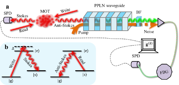
Figure 1: Schematic view of the experimental setup. a, A cold cloud of ${}^{87}\mathrm{Rb}$ atoms confined in a magneto-optical trap (MOT) serves as quantum memory for light. Inelastic scattering of a classical write pulse results in the emission of a Stokes photon, which heralds the presence of a collective spin excitation. A subsequent read pulse maps the atomic state onto an anti-Stokes photon. The retrieved light is sent to a PPLN waveguide, together with a strong pump at $1569\,\mathrm{nm}$. The $780\,\mathrm{nm}$ photons are converted to $1552\,\mathrm{nm}$ by DFG. After conversion, residual pump light is blocked by means of a bandpass filter (BF). The converted light is then coupled in a single mode optical fiber. A fiber Bragg grating filters out the broadband noise generated by the pump. The non classical nature of the storage, retrieval and conversion processes is probed by measuring the cross-correlation between Stokes and (un)converted anti-Stokes photons. b, Level scheme used for the DLCZ memory. The write pulse off-resonantly couples the ground state $\left|g\right\rangle$ to the excited level $\left|e\right\rangle$. A Stokes photon is emitted with probability $p$, thus creating a single collective excitation to the storage state $\left|s\right\rangle$. During the retrieval process, a pulse resonant with the $\left|s\right\rangle\rightarrow\left|e\right\rangle$ transition (read beam) collectively transfers back the atom to the initial state $\left|g\right\rangle$.

In this paper we demonstrate an ultra low noise solid state photonic quantum interface capable of connecting QMs based on atomic ensembles to the telecommunication network. We generate heralded single photons at $780\,\mathrm{nm}$ from a cold $\mathrm{{}^{87}Rb}$ atomic ensemble QM and convert them to $1552\,\mathrm{nm}$ using frequency down conversion in a non linear periodically poled lithium niobate (PPLN) waveguide. By combining high QM retrieval efficiency, high QFC efficiency and narrow band filtering, we can operate the combined systems in a regime where a significant amount of non classical correlations is preserved between the heralding and converted photons.

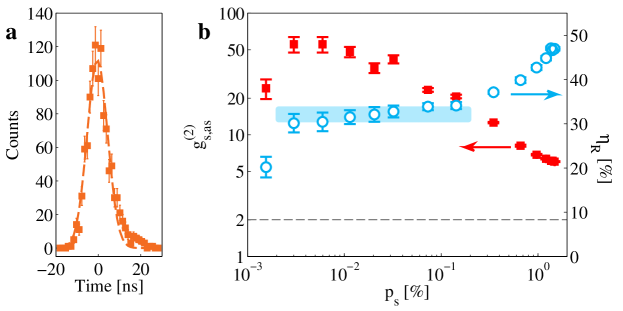
Figure 2: Characterization of the DLCZ quantum memory. a, Temporal shape of anti-Stokes photons. The number of anti-Stokes detection events per time bin (bin size $1.28\,\mathrm{ns}$) conditioned on a Stokes detection over $5\times 10^{6}$ trials is plotted as a function of the arrival time (orange squares). The data shown correspond to $p_{s}=0.15\,\%$. The dashed line is a gaussian fit with $\mathrm{FWHM}=11.4(9)\,\mathrm{ns}$. For this data, we have $g^{(2)}_{s,as}=22(1)$ and $\eta_{R}=35(1)\,\%$. b Second-order cross-correlation function $g^{(2)}_{s,as}$ (red plain squares, left axis) and retrieval efficiency $\eta_{R}$ (blue empty circles, right axis) as a function of the Stokes detection probability $p_{s}$. For $p_{s}$ between $0.002$ and $0.2\,\%$ (shaded area), $\eta_{R}$ is constant ($32(2)\%$). The $g^{(2)}_{s,as}$ function increases until $56(8)$, before dropping for lower values of $p_{s}$ due to detector dark counts. The dashed line is the $g^{(2)}_{s,as}$ classical limit for two mode squeezed states.

II Results

II.1 The atomic quantum memory

Our experimental setup is shown in Fig. 1 (see Appendix A for details). It is composed of two main parts, the QM and the quantum frequency conversion device (QFCD). The QM is implemented with an ensemble of laser cooled $\mathrm{{}^{87}Rb}$ atoms, following the scheme proposed by Duan, Lukin, Cirac and Zoller Duan2001 . Single collective spin excitations are created by a $16\,\mathrm{ns}$ long weak write pulse at $780\,\mathrm{nm}$, blue detuned by $40\,\mathrm{MHz}$ from the $\left|g\right\rangle$ to $\left|e\right\rangle$ transition, and heralded by the detection of a photon emitted by spontaneous Raman scattering, called Stokes photon. The collective spin excitation is stored in the atoms for a programmable time ($330\,\mathrm{ns}$ in our experiment) before being transferred back into a single photon (anti-Stokes) thanks to an $11\,\mathrm{ns}$ long read laser pulse resonant with the $\left|s\right\rangle$ to $\left|e\right\rangle$ transition. The anti-Stokes photon is emitted with high efficiency in a single spatio-temporal mode thanks to collective interference between all the emitters. It is then coupled with high efficiency ($0.7$) into a single mode fiber before being detected by a single photon detector (SPD) with efficiency $\eta_{d,780}=0.43$.

Figure 2a shows the temporal profile of the heralded retrieved anti-Stokes field. We measure a full width at half maximum ($\mathrm{FWHM}$) of $11.4(9)\mathrm{ns}$, shorter than previous single photons generated by the same method Felinto2006 ; Bao2012 . We then characterize the non classical correlations between the Stokes photons and the stored spin excitations. This is realized by measuring the second order cross-correlation function $g^{(2)}_{s,as}$ between the Stokes and anti-Stokes fields, defined as $g^{(2)}_{s,as}=p_{s,as}/(p_{s}p_{as})$, where $p_{s,as}$ is the probability to detect a coincidence between the two modes and $p_{s}$ ($p_{as}$) is the probability to detect a Stokes (anti-Stokes) photon. $p_{s}$ is proportional to the write pulse intensity. Figure 2b shows a typical measurement of $g^{(2)}_{s,as}$ as a function of $p_{s}$. As expected for this type of source, the degree of correlation increases when decreasing the excitation probability Laurat2006 . The measured $g^{(2)}_{s,as}$ is well above the classical threshold of $2$ for two-mode squeezed states (see Appendix D). This suggests that strong non classical correlations between the Stokes photon and the stored spin excitation are present. Additional measurements demonstrating the non classical character of the correlations are shown in Appendix D (see also Table 1). Also shown in Fig. 2b is the retrieval efficiency $\eta_{R}=p_{s,as}/(p_{s}\eta_{d,780})$ corresponding to the probability to find an anti-Stokes photon before the SPD conditioned on the detection of a Stokes photon. In the region where the multi-excitation probability and the Stokes detector dark counts are negligible Laurat2006 ($p_{s}$ between $0.002\,\%$ and $0.2\,\%$), $\eta_{R}$ is constant and equal to $32(2)\,\%$ (shaded area on Fig. 2b).

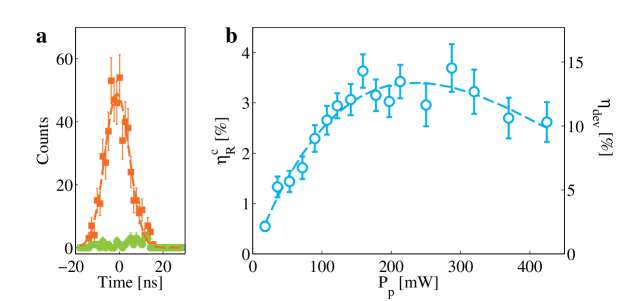
Figure 3: Characterization of the quantum frequency conversion device a, Converted anti-Stokes photon shape. The conditioned events are plotted as orange squares, while the conditioned pump noise is shown as green circles. The measured signal to noise ratio is $18(5)$. The time bin size is $1.28\,\mathrm{ns}$. The Stokes detection probability for the measurement is $p_{s}=0.16\,\%$ while the pump power is $P_{p}=120\,\mathrm{mW}$. For this measurement, we have $g^{(2)c}_{s,as}=11.6(7)$ and $\eta_{R}^{c}=3.4(2)\,\%$ b Conversion efficiency as a function of pump power after the waveguide measured with heralded anti-Stokes photons. The right axis shows the device efficiency $\eta_{\mathrm{dev}}$ corresponding to raw conversion efficiency corrected only by the detection efficiency ($0.1$). The left axis shows $\eta_{R}^{c}=\eta_{R}^{in}\eta_{\mathrm{dev}}$, i.e. the probability to find a converted photon before the SPD, conditioned on a Stokes detection. The Stokes detection probability for this measurement is $p_{s}=0.16\,\%$.

II.2 The Quantum Frequency Converter Device

The heralded anti-Stokes single photon is then directed towards the QFCD where the conversion from $780\,\mathrm{nm}$ to $1552\,\mathrm{nm}$ takes place. From the measured $\eta_{R}$ and the optical transmission between the QM and the QFCD ($\eta_{\mathrm{loss}}=0.77$), we infer that, conditioned on a Stokes detection, the number of photons before the QFCD is $\eta^{in}_{R}=\eta_{R}\eta_{\mathrm{loss}}=0.25(2)$. The pump light at $1569\,\mathrm{nm}$ and the single photons at $780\,\mathrm{nm}$ are combined using a dichroic mirror. Both beams are then coupled into the waveguide where the conversion takes place. After conversion, the pump light is blocked by means of two bandpass filters, and the converted light is coupled into a single mode optical fiber. A fiber Bragg grating with a bandwidth of $2.5\,\mathrm{GHz}$ and a transmission efficiency of $0.7$ then filters out the broadband noise generated in the crystal by the pump beam Fernandez-Gonzalvo2013 . The single photons at $1552\,\mathrm{nm}$ are finally detected with an InGaAs avalanche photodiode SPD (detection efficiency $\eta_{d,1552}=0.1$).

Figure 3a shows the waveform of the heralded single photons after conversion. The measured temporal profile ($\mathrm{FWHM}=13(1)\,\mathrm{ns}$) is very similar to the input one, which shows that the conversion preserves the waveform of the photons. The noise generated by the pump beam at $1569\,\mathrm{nm}$ is measured by blocking the input of the converter. The measured signal to noise ratio ($\mathrm{SNR}$) of $18(5)$ gives an upper bound for the value of the cross correlation function $g^{(2)c}_{s,as}$ achievable after conversion (see Appendix C). We also measure the efficiency of the conversion process as a function of the pump power $P_{p}$ measured after the waveguide. Figure 3b shows the device efficiency $\eta_{\mathrm{dev}}=p_{s,as}^{c}/(p_{s}\eta_{R}^{in}\eta_{d,1552})$, where $p_{s,as}^{c}$ is the probability to detect a coincidence after conversion. $\eta_{\mathrm{dev}}$ corresponds to the probability to find a converted photon in a single mode optical fiber after the QFCD (including filtering and fiber coupling) for a single photon input. The data are fitted with the following formula $\eta_{\mathrm{dev}}=\eta_{\mathrm{max}}\sin^{2}(L\sqrt{\eta_{n}P_{p}})$ Zaske2011 . From the fit, we extract $\eta_{n}=120(10)\,\mathrm{\%W^{-1}cm^{-2}}$ and $\eta_{\mathrm{max}}=13.6(12)\,\%$. The maximum achievable device efficiency is limited in our current setup to $17.6\,\%$ by optical losses, including fiber coupling efficiency($60\,\%$) and Bragg grating filter transmission ($70\,\%$) at the converted wavelength of $1552\,\mathrm{nm}$, as well as by the waveguide incoupling ($60\,\%$) and transmission ($70\,\%$) efficiencies for $780\,\mathrm{nm}$ photons. The discrepancy between the measured $\eta_{\mathrm{max}}$ and the theoretical one is attributed to non perfect mode overlap between the pump and single photon in the waveguide Zaske2011 . Figure 3b also displays $\eta_{R}^{c}=\eta_{R}^{in}\eta_{\mathrm{dev}}$, which can be considered as the combined efficiency of the QM+QFCD system, including all losses.

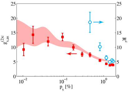
Figure 4: Characterization of the quantum memory–quantum frequency converter combined setup. Cross-correlation between Stokes and converted anti-Stokes photons as a function of Stokes detection probability, for a pump power of $140\,\mathrm{mW}$ (red plain squares, left axis). The shaded area represents the expected $g^{(2)c}_{s,as}$ deduced from the data of Fig. 2b by means of equation (1) (see Appendix B). The measured Cauchy-Schwartz parameter $R^{c}$ is plotted on the right axis (blue empty circles). The unconditional autocorrelation measurement for the converted anti-Stokes field has been measured for a pump power of $120\,\mathrm{mW}$.

II.3 Quantum state preservation

In order to verify that the conversion preserves the quantum character of the input light, we measure the second order cross-correlation function after conversion $g^{(2)c}_{s,as}$ as a function of $p_{s}$ (see Fig. 4). As in the case before conversion (Fig. 2b), we also observe an increase of non classical correlations when decreasing the excitation probability, but the maximum is now reached for much higher values of $p_{s}$ because of the background noise induced by the converter pump laser. However, this background is sufficiently low to observe strong non classical correlations between the heralding photons at $780\,\mathrm{nm}$ and the converted photons at $1552\,\mathrm{nm}$. The expected value of the $g^{(2)c}_{s,as}$ after conversion can be estimated using a simple model taking into account the noise induced by the pump laser, using the following expression (see Appendix B):

$$g^{(2)c}_{s,as}=g^{(2)}_{s,as}\frac{\mathrm{SNR}+1}{\mathrm{SNR}+g^{(2)}_{s,as}}$$ (1)

The shaded area displayed in Fig. 4 corresponds to the expected values taking into account the $g^{(2)}_{s,as}$ measured in Fig. 2 and $\mathrm{SNR}=\eta_{R}^{in}\cdot\mathrm{SNR}^{\mathrm{max}}$, where $\mathrm{SNR}^{\mathrm{max}}$ is the maximal achievable $\mathrm{SNR}$ for $\eta_{R}^{in}=1$ and can be accurately measured with weak coherent states (see Appendix B). We find $\mathrm{SNR}^{\mathrm{max}}=85(3)$. The good agreement between experimental data and expected values suggests that the noise generated from the pump is the only factor degrading the correlations and that further reduction of this noise should lead to even higher non classical correlations.

Finally, in order to unambiguously prove the non classical character of the correlations, we also measure the unconditional auto correlation function for the Stokes ($g^{(2)}_{s,s}=p_{s,s}/(p_{s}p_{s}))$ and converted anti-Stokes fields ($g^{(2)c}_{as,as}=p_{as,as}^{c}/(p_{as}^{c}p_{as}^{c}))$. For classical independent fields, the Cauchy-Schwartz inequality $R^{c}=\left(g^{(2)c}_{s,as}\right)^{2}/\left(g^{(2)}_{s,s}\cdot g^{(2)c}_{as,as}\right)\leq 1$ must be satisfied. The values for $g^{(2)}_{s,s}$ and $g^{(2)c}_{as,as}$ are listed in Table 1. On the right axis of Fig. 4 we plot the values of $R^{c}$ measured in our experiment for various $p_{s}$. The Cauchy-Schwartz inequality is clearly violated, which is a proof of non classical correlation between Stokes and converted anti-Stokes photons.

III Discussion

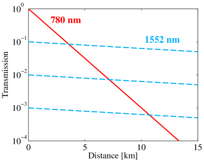
Figure 7: Comparison between transmissions of converted and unconverted photons. Transmission of $780\,\mathrm{nm}$ light in a telecom fiber as a function of the propagation distance assuming losses of $\sim 3\,\mathrm{dB/km}$ (red continuous line). Similarly, the blue dashed lines represent transmission of $1552\,\mathrm{nm}$ converted photons with $10$, $1$ and $0.1\,\%$ device efficiency, assuming propagation losses of $\sim 0.2\,\mathrm{dB/km}$. As it can be seen, even for a device efficiency as low as $0.1\,\%$, the limited conversion efficiency is compensated after only $11\,\mathrm{km}$ of propagation through the fiber.

We now discuss the performances of our interface. The maximal $g^{(2)c}_{s,as}$ obtained is about $15$, which would be sufficient to enable a violation of Bell’s inequality if the photons were entangled Riedmatten2006 . The measured maximal $\eta_{\mathrm{dev}}=13.6(12)\,\%$ corresponds to an internal waveguide conversion efficiency of $77\,\%$. As it is, it would already lead to an increased transmission with respect to the unconverted photon at $780\,\mathrm{nm}$ ($3\,\mathrm{dB/km}$ loss) after only $\sim 3\,\mathrm{km}$ of fiber (see also Fig. 7). Further improvement in the device efficiency could be primarily obtained by technical improvements such as decreasing the passive optical losses due to waveguide coupling and transmission, fiber coupling and filtering transmission.

Our quantum photonic interface could be directly useful for some efficient quantum repeater architectures using DLCZ type QMs, where entanglement between remote quantum nodes is achieved by entanglement swapping involving the anti-Stokes photons Sangouard2008a . In that case, the anti-Stokes photons are sent over long distances and must thus be converted to telecom wavelengths. For protocols where entanglement between remote atomic ensembles is achieved by detection of the Stokes photon, such as the original DLCZ protocol Duan2001 , or in order to achieve entanglement between a telecom photon and a stored spin excitation, the Stokes photon should then be converted. This would however require a significant increase of the $\mathrm{SNR}$ compared to our present experiment, since the Stokes emission probability has to be low to allow highly non classical correlations. This reduction may be achieved by using narrower filtering since the current value of $2.5\,\mathrm{GHz}$ is about two order of magnitude larger than the photon bandwidth. Obtaining higher $\mathrm{SNR}$ would be also interesting in view of using this interface in combination with single atom QMs emitting photons with duration of a few hundred $\mathrm{ns}$ Ritter2012 .

We have demonstrated quantum frequency conversion to telecommunication wavelength of single photons emitted by a quantum memory, using a solid state integrated photonic quantum interface. These results open the road to the use of integrated optics as a practical and flexible interface capable of connecting QMs to the optical fiber network. The wavelength flexibility offered by non linear crystals opens the door to QFC with other kind of QMs, such as solid state QMs Riedmatten2008 ; Hedges2010 ; Clausen2011 ; Saglamyurek2011 or single ions Moehring2007 . Our work is a step to extend quantum information networks to long distances and opens prospects for the coupling of different types of remote QMs via the optical fiber network.

Appendix A Atomic ensemble based quantum memory

Our quantum memory (QM) is based on an ensemble of rubidium atoms, trapped and cooled in a magneto optical trap (MOT) operating on the $\mathrm{D2}$ line of ${}^{87}\mathrm{Rb}$ at $780\,\mathrm{nm}$. The optical depth (OD) of the sample is measured to be $\sim 12$, when probing the $\left|5\,{}^{2}S_{1/2},F=1\right\rangle\rightarrow\left|5\,{}^{2}P_{3/2},F^{\prime}=2\right\rangle$ transition. At the beginning of the experimental sequence the MOT is turned off and the atoms are optically pumped during $300\,\mathrm{\mu s}$ into the ground state $\left|g\right\rangle=\left|5\,{}^{2}S_{1/2},F=1\right\rangle$. The initial state of the system is described by $\left|G\right\rangle=\left|g_{1}\dots g_{N}\right\rangle$, $N$ being the atom number. A weak laser pulse (write beam), linearly polarized and blue detuned by $40\,\mathrm{MHz}$ with respect to the $\left|g\right\rangle\rightarrow\left|e\right\rangle$ transition ($\left|e\right\rangle$ being the excited state $\left|5\,{}^{2}P_{3/2},F^{\prime}=2\right\rangle$), is then sent to the cold cloud. The write beam has a waist of $\sim 150\,\mathrm{\mu m}$ and the pulse is characterized by a full width at half maximum ($\mathrm{FWHM}$) of $16\,\mathrm{ns}$. Raman scattering of the write beam induces the transfer of one atom to the storage level $\left|s\right\rangle=\left|5\,{}^{2}S_{1/2},F=2\right\rangle$, with low probability. This process is followed by the emission of a photon on the $\left|e\right\rangle\rightarrow\left|s\right\rangle$ transition (Stokes photon), which is collected by means of a $500\,\mathrm{mm}$ focal length lens and then coupled into a single mode optical fiber. The collection mode corresponds to a waist of $\sim 50\,\mathrm{\mu m}$, such that the observed region is smaller than the volume illuminated by the write beam. We indicate with $p$ the probability for a Stokes photon to be emitted in the collection mode. The emitted light is finally detected by a Si avalanche photodiode (Count-100C-FC, Laser components), characterized by a measured detection efficiency of $\sim 43\%$ at $780\,\mathrm{nm}$ and a dark count rate of $100\,\mathrm{Hz}$. The single photon detector (SPD) is operated in gated mode with a detection window of $40\,\mathrm{ns}$.

Since the Stokes photons are emitted while the write pulse is on, it is necessary to filter the Stokes field from the possible leakage of the classical beam. For this purpose three strategies are employed: (a) polarization, (b) angular and (c) frequency filtering (see Fig. 5 for a schematic view of the experimental setup). (a) By means of a half waveplate and a polarizing beam splitter cube, we ensure to detect only Stokes photons orthogonally polarized with respect to the write beam. (b) The detection mode is aligned with an angle of $3$ degrees with respect to the write mode, thus avoiding direct coupling of the classical light into the collection fiber. (c) In between the atomic cloud and the SPD we place a monolithic Fabry-Perot cavity characterized by a $\mathrm{FWHM}$ of $\sim 60\,\mathrm{MHz}$ and a free spectral range (FSR) of $\sim 12\,\mathrm{GHz}$. The cavity is formed by a plano-concave lens coated on both sides with a high reflectivity layer at $780\,\mathrm{nm}$, following the design described by Palittapongarnpim et al. Palittapongarnpim2012 . The Stokes photons are delivered by an optical fiber to a free-space setup where they are shaped to match the $\mathrm{TE_{00}}$ mode of the resonator. The cavity length is tuned by acting on the lens temperature and is adjusted to be resonant with the Stokes photons. The cavity transmission is $\sim 50\%$ when measured with monochromatic light. Considering that our Stokes photons have a spectral bandwidth of about $40\,\mathrm{MHz}$ (i.e. $\mathrm{FWHM}$ of $11\,\mathrm{ns}$) their transmission through the resonator is limited to $\sim 80\%$. The maximum cavity transmission is then $\sim 40\,\%$. The photons filtered by the resonator are then coupled into another fiber connected to the SPD. The total transmission of the system, including losses and fiber in-coupling efficiency, is measured to be $\sim 25\,\%$ when probed with continuous light (i.e. $20\,\%$ for the Stokes photons). The write beam is detuned with respect to the Stokes field by $6.8\,\mathrm{GHz}$ (i.e. the hyperfine splitting between the $\left|g\right\rangle$ and $\left|s\right\rangle$ levels) which corresponds to about half the FSR of the cavity. This ensures that its transmission through the resonator is below $1\,\%$. The combination of the three filtering methods described above allows us to reduce the noise caused by the write light to a level lower than the dark count rate of the SPD.

The probability to detect a Stokes photon is indicated as $p_{s}$ and it is given by $\eta_{s}\times p$, where the factor $\eta_{s}=6\,\%$ accounts for the coupling efficiency of the Stokes mode into the optical fiber ($0.7$, see later for details), the filter cavity transmission ($\sim 0.2$) and the detection efficiency ($0.43$). The Stokes creation probability $p$ can be varied acting on the write power. In our experiment $p$ is spanned over three orders of magnitude from $2.5\times 10^{-4}$ to $0.25$ (i.e. $p_{s}$ varies from $1.5\times 10^{-5}$ to $1.5\times 10^{-2}$). The detection of a Stokes photon projects the system onto the collective state:

$$\left|S\right\rangle=\frac{1}{\sqrt{N}}\sum\limits_{j=1}^{N}\exp{\left[\imath(\vec{k}_{w}-\vec{k}_{s})\cdot\vec{x}_{j}\right]}\left|g_{1}\dots s_{j}\dots g_{N}\right\rangle,$$ (2)

where $\vec{x}_{j}$ is the position of the $j$-th atom, while $\vec{k}_{w}$ and $\vec{k}_{s}$ are the wavevectors for the write and Stokes modes, respectively. This is a good description of the system only under the assumption of low excitation probability (i.e. $p\ll 1$), such that multiple excitations can be neglected. This process can be regarded as a heralded generation of a single spin excitation in the atomic ensemble.

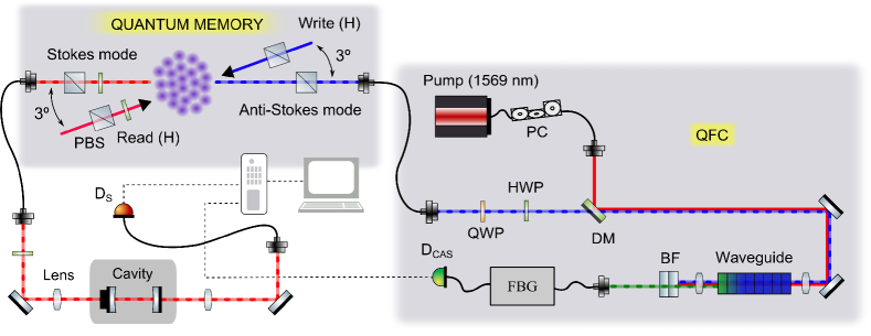
Figure 5: Schematic view of the experimental setup. See text for a detailed description of the different components.

After a programmable delay $\tau_{s}$ ($330\,\mathrm{ns}$ for our experiment), a bright light pulse (read beam) resonantly couples the $\left|s\right\rangle$ and $\left|e\right\rangle$ states, thus transferring back the population to the ground level $\left|g\right\rangle$. The pulse propagates in the same spatial mode as the write beam but in the opposite direction. The peak power of $\sim 800\,\mathrm{\mu W}$ and the $\mathrm{FWHM}$ of $11\,\mathrm{ns}$ have been chosen in order to maximize the transfer efficiency Mendes2013 . The retrieval process is accompanied by the collective re-emission of a photon on the $\left|e\right\rangle\rightarrow\left|g\right\rangle$ transition (anti-Stokes photon). At the end of the sequence the collective state of the system is:

$$\left|G^{\prime}\right\rangle=\frac{1}{\sqrt{N}}\sum\limits_{j=1}^{N}\exp{\left[\imath(\vec{k}_{w}-\vec{k}_{s})\cdot\vec{x}_{j}\right]}\exp{\left[\imath(\vec{k}_{r}-\vec{k}_{as})\cdot\vec{x}_{j}^{\prime}\right]}\left|g_{1}\dots g_{j}\dots g_{N}\right\rangle,$$ (3)

where $\vec{x}_{j}^{\prime}$ is the final position of the $j$-th atom, while $\vec{k}_{r}$ and $\vec{k}_{as}$ are the wavevectors for the read and anti-Stokes modes respectively. For a sample temperature of the order of a few hundreds of micro Kelvin and a storage time below $1\,\mathrm{\mu s}$, the atomic motion is negligible during the storing process and $\vec{x}_{j}^{\prime}\simeq\vec{x}_{j}$. In this case, the final state $\left|G^{\prime}\right\rangle$ coincides with the initial state $\left|G\right\rangle$ if the phase matching condition $\vec{k}_{w}-\vec{k}_{s}=\vec{k}_{as}-\vec{k}_{r}$ is satisfied. For our excitation geometry this implies that the anti-Stokes photon is emitted in the same mode as for the Stokes photon but in opposite direction (i.e. $\vec{k}_{as}=-\vec{k}_{s}$). The single spin excitation created in the ensemble during the write process is then collectively read-out and mapped onto the anti-Stokes photon.

The retrieved photons are coupled into an optical fiber. The overlap between the Stokes and anti-Stokes modes is estimated to be $\sim 70\%$ by measuring the fiber to fiber coupling using classical light. The photons are then delivered to a second SPD with similar specifications as the first one (SPCM-AQRH-14-FC, Excelitas), temporally gated for $40\,\mathrm{ns}$. Polarization and angular filtering are used to reduce the leakage of the read beam as for the Stokes detection. In this case, however, we do not use a cavity for frequency filtering, in order to maximize the retrieval efficiency. This is crucial when the system is used in combination with the quantum frequency converter device (QFCD).

A clean pulse with the same frequency and spatial mode as the read beam is sent to the atomic cloud in order to efficiently pump all the atoms back to the initial state $\left|g\right\rangle$, while the SPDs are kept off. The write–read sequence is repeated $1000$ times, each trial lasting $\Delta\tau=1.4\,\mathrm{\mu s}$. During the total interrogation time of $1.4\,\mathrm{ms}$ the atomic cloud is falling freely under the effect of gravity. During this short time the OD reduction due to cloud expansion is negligible. We can therefore assume that all the trials are performed under the same conditions. The trap and repumper beams as well as the magnetic field gradient are then switched on and the atoms are recaptured in the MOT, where they are laser cooled during $20\,\mathrm{ms}$ before the sequence starts again. This full cycle is repeated until a good statistic is reached.

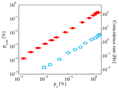
Figure 6: Heralded anti-Stokes generation rates. The probability $p_{s,as}$ to detect a Stokes–anti-Stokes coincidence per trial is plotted as a function of the Stokes detection probability $p_{s}$ for the memory alone (red plain squares) and in combination with the QFCD (blue empty circles). On the right axis the corresponding detection rates are also plotted.

Due to the strong correlations between the Stokes photon and the single spin excitation created in the system, if we assume that the read-out process is performed with high efficiency, we can describe the joint state of the Stokes and anti-Stokes photons as:

$$\begin{split}\left|\psi\right\rangle=&\left(1-\frac{p}{2}\right)\left|0_{s},0_{as}\right\rangle+\\ &+\sqrt{p}\left|1_{s},1_{as}\right\rangle+\\ &+p\left|2_{s},2_{as}\right\rangle+O\left(p^{3/2}\right).\end{split}$$ (4)

This ideal two-mode squeezed state displays a high degree of second order cross-correlations between the Stokes and anti-Stokes fields. The second order cross-correlation function $g^{(2)}_{s,as}$ is defined as $p_{s,as}/\left(p_{s}p_{as}\right)$, where $p_{s}$ and $p_{as}$ are the probabilities to detect a Stokes and an anti-Stokes photons per trial, respectively. The quantity $p_{s}\cdot p_{as}$ can be interpreted as the probability to get an accidental coincidence. On the other hand, $p_{s,as}$ is the probability to detect an anti-Stokes photon conditioned on the detection of a Stokes photon in the same write-read trial (i.e the Stokes–anti-Stokes coincidence probability). In Fig. 6, $p_{s,as}$ is plotted as a function of the Stokes detection probability $p_{s}$, together with the coincidence rate achievable in the experiement. In order to measure the $g^{(2)}_{s,as}$ function, the outputs of the two SPDs are acquired by a time-stamping card which records their arrival times. Correlated photons are emitted within the same write–read trial and therefore their relative arrival time is given by $\tau_{s}$. On the other hand, Stokes and anti-Stokes photons generated in different trials will arrive with a time difference $\tau_{s}+n\cdot\Delta\tau$, with $n$ integer. The ratio between the number of coincidences with an arrival time of $\tau_{s}$ and $\tau_{s}+\Delta\tau$ is therefore a measurement of the second order cross-correlation function.

Appendix B Quantum frequency converter

Our quantum frequency converter is based on difference frequency generation (DFG) of $1552\,\mathrm{nm}$ light, achieved by combining input photons at $780\,\mathrm{nm}$ with a strong pump at $1569\,\mathrm{nm}$ in a periodically poled lithium niobate (PPLN) waveguide. Our current experimental setup (see Fig. 5) is based on the apparatus described in Fernandez-Gonzalvo2013 . Thanks to the introduction of a new filtering stage the noise contribution has been reduced by more than one order of magnitude with respect to our previous work. This achievement, together with an improvement of the device efficiency and the use of shorter photons, allowed us to increase the signal to noise ratio of the conversion process by almost two orders of magnitude (see later for details). In the following, after a brief description of the main parts of the setup, we will focus on the characteristics of the new spectral filter, suggesting the reader to refer to our previous work for an exhaustive description of the other elements.

The input photons at $780\,\mathrm{nm}$ are combined on a dichroic beam splitter together with the pump light, obtained from an erbium doped fiber amplifier feeded by an external cavity diode laser. The two light fields are then coupled to the nonlinear waveguide by means of an aspheric lens. The measured coupling efficiencies are $68\%$ and $60\%$ for the pump and input modes, respectively. The input lens has a transmission of $\sim 66\,\%$ at $1569\,\mathrm{nm}$. The specified waveguide transmissions are about $62\,\%$ and $78\,\%$ at the input and pump wavelengths, respectively. At the waveguide output, two band pass filters with a $\mathrm{FWHM}$ of $7\,\mathrm{nm}$ isolate the converted signal from the residual pump light. Each filter has a transmission of $93\,\%$ at $1552\,\mathrm{nm}$, while it displays an OD of $\sim 12$ at $1569\,\mathrm{nm}$. This filtering stage is not sufficient to reduce the noise around the converted wavelength of $1552\,\mathrm{nm}$ below the single photon level. The strong pump light generates additional noise whose broadband nature has been investigated in Fernandez-Gonzalvo2013 . In particular, we measured that the residual noise level is proportional to the spectral bandwidth of the filtering stage (see also kuo2013 ).

Guided by this observation, we replaced our previous filtering stage, based on a simple diffraction grating, with a fiber Bragg grating. The current filter linewidth of $2.5\,\mathrm{GHz}$ is $34$ times narrower than the minimum we could achieve with the previous setup. When the QM is used in combination with the QFCD, the fiber Bragg grating helps filtering the residual leakage of the read beam, like the monolithic resonator used for the Stokes photon. Considering the coupling efficiency of the input light into the waveguide ($60\,\%$), the intrinsic losses in the waveguide ($70\,\%$, corresponding to the geometric average of the losses experienced at $780\,\mathrm{nm}$ and $1552\,\mathrm{nm}$), the fiber coupling efficiency ($60\%$) and the transmission of the filtering elements ($70\%$), the achievable total efficiency is limited to $17.6\,\%$. The converted light is finally sent to an InGaAs SPD (id220, Id Quantique), with a detection efficiency of $10\%$ and a dark count rate of $400\,\mathrm{Hz}$ with a dead time of $20\,\mathrm{\mu s}$.

B.1 QFCD characterization

In order to characterize the QFCD, we use weak coherent pulses at $780\,\mathrm{nm}$ with a $\mathrm{FWHM}$ of $14\,\mathrm{ns}$, to simulate the anti-Stokes photons obtained from our QM. We measure the device efficiency and the signal to noise ratio for the converted light as a function of the pump power. The results are shown in Fig. 8a. The device efficiency varies as a function of the pump power $P_{p}$ as:

$$\eta_{\mathrm{dev}}=\eta_{\mathrm{max}}\times\sin^{2}\left(L\sqrt{P_{p}\eta_{n}}\right),$$ (5)

where $\eta_{\mathrm{max}}$ is the maximum achievable efficiency, $L$ is the crystal length and $\eta_{n}$ is the normalized conversion efficiency Zaske2011 . Fitting the experimental data with equation (5), we find $\eta_{\mathrm{max}}=11.4(4)\,\%$ and $\eta_{n}=119(9)\,\mathrm{\%W^{-1}cm^{-2}}$. These values are compatible with the corresponding ones obtained with quantum light at the device input and described in the main paper. Despite the limited device efficiency measured in the experiment, our QFCD already offers a significant advantage over direct transmission of $780\,\mathrm{nm}$ photons over long distances, as it is shown in Fig. 6.

An analogous formula can be derived for the signal to noise ratio Fernandez-Gonzalvo2013 . We define the signal $s$ as $\mu_{in}\cdot\eta_{\mathrm{dev}}\cdot\eta_{d,1552}$, where $\mu_{in}$ is the mean input photon number per pulse and $\eta_{d,1552}$ is the detection efficiency ($0.1$). The quantity $s$ can be interpreted as the probability to get a click on the detector due to a converted photon. On the other hand, the probability to detect a noise photon is proportional to the pump power, i.e. $n=\delta n\cdot P_{p}$. We therefore obtain:

$$\mathrm{SNR}=\frac{s}{n+\mathrm{dc}},$$ (6)

where $dc$ is the dark count probability. For low pump powers, the device efficiency $\eta_{\mathrm{dev}}$ decreases (see equation (5)), thus causing a reduction of $s$. On the other hand, the noise is limited to the dark count level $\mathrm{dc}$. As a consequence, the $\mathrm{SNR}$ drops to zero. When $P_{p}$ increases, the $\mathrm{SNR}$ increases as well until a maximum is reached. A further increase of the pump power will result in a decrease of the $\mathrm{SNR}$, since the noise keeps on increasing while the device efficiency saturates. This behavior can clearly be observed in Fig. 8a. For the experiment described in the main paper we used a pump power of about $120\mathrm{mW}$ in order to operate the device close to the point where the $\mathrm{SNR}$ is the highest.

As it will be detailed in the next section, the $\mathrm{SNR}$ is the key parameter to estimate the $g^{(2)c}_{s,as}$ value achievable after conversion. It is therefore important to have a good estimate of its value. For this purpose, we measure the $\mathrm{SNR}$ as a function of $\mu_{in}$ for a fixed pump power. As it is shown in Fig. 8b, the $\mathrm{SNR}$ is linearly proportional to $\mu_{in}$, i.e. $\mathrm{SNR}=\mathrm{SNR^{max}}\times\mu_{in}$. The proportionality constant $\mathrm{SNR^{max}}$ can be regarded as the maximum achievable $\mathrm{SNR}$ when the system is operated with a single photon input (i.e. $\mu_{in}=1$). A fit to the experimental data give us $\mathrm{SNR^{max}}=85(3)$. This value is a factor $\sim 70$ higher than what has been reported in Fernandez-Gonzalvo2013 . This result has been achieved thanks to the improvement of the noise filtering, the increase of the device efficiency and the use of shorter photons.

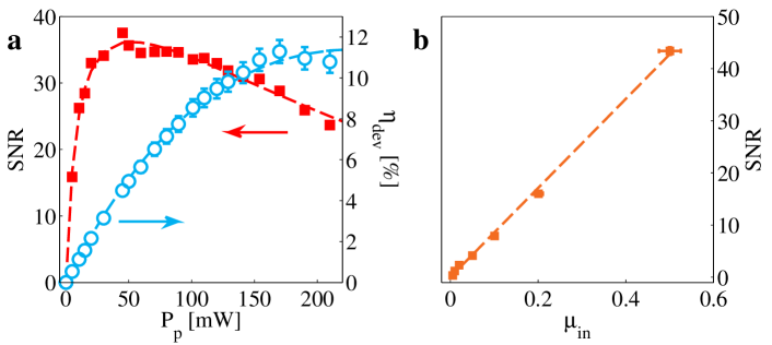
Figure 8: QFCD characterization. a, Signal to noise ratio (red plain squares, left axis) and device efficiency (blue open circles, right axis) as a function of the pump power (measured at the waveguide output) for $\mu_{\mathrm{in}}=0.37$. The dashed blue line corresponds to a fit of $\eta_{\mathrm{dev}}$ data using equation (5). The fit gives $\eta_{\mathrm{max}}=11.4(4)\,\%$ and $\eta_{n}=119(9)\,\mathrm{\%W^{-1}cm^{-2}}$. The dashed red line corresponds to a fit of the $\mathrm{SNR}$ data using equation (6). b, Signal to noise ratio as a function of the mean input photon number $\mu_{\mathrm{in}}$ for $P_{p}\sim 120\,\mathrm{mW}$ (measured at the waveguide output). A linear fit of the data (dashed orange line) gives $\mathrm{SNR^{max}}=85(3)$.

Appendix C Expected second order cross-correlation function

The second order cross-correlation function between the Stokes and anti-Stokes fields experiences a reduction when the frequency of the anti-Stokes photons is translated to the telecom band by means of our QFCD, due to the presence of the broadband noise generated by the pump. In this section we will detail the derivation of equation 1 of the main paper, which allows us to quantify this reduction.

The anti-Stokes detection probability after conversion can be expressed by $p_{as}^{c}=\eta_{\mathrm{tot}}\cdot p_{as}+p_{n}$, where $p_{as}$ is the probability to detect an unconverted anti-Stokes photon, while $p_{n}$ is the probability to detect a noise photon. The quantity $\eta_{\mathrm{tot}}=\eta_{\mathrm{dev}}\eta_{\mathrm{loss}}\cdot(\eta_{d,1552}/\eta_{d,780})$ accounts for the QFCD efficiency ($\eta_{\mathrm{dev}}$), the passive losses between the anti-Stokes fiber output and the QFCD input ($\eta_{\mathrm{loss}}\sim 0.77$) and the difference between the efficiencies of the single photon detectors used for $780\,\mathrm{nm}$ ($\eta_{d,780}=0.43$) and $1552\,\mathrm{nm}$ ($\eta_{d,1552}=0.1$). The probability to detect an accidental coincidence between the Stokes and anti-Stokes fields is defined as $p_{as}^{c}\cdot p_{s}$ and it is therefore given by $\eta_{\mathrm{tot}}\cdot p_{s}\cdot p_{as}+p_{n}\cdot p_{s}$. On the other hand, the coincidence probability $p_{s,as}^{c}$ will be given by $\eta_{\mathrm{tot}}\cdot p_{s,as}+p_{n}\cdot p_{s}$. The factor $\eta_{\mathrm{tot}}$ is the same as for $p_{as}$, while the quantity $p_{n}\cdot p_{s}$ can be regarded as the probability to detect a noise photon conditioned on a previous detection of a Stokes photon (conditional noise). Using the definition of the second order cross-correlation function we obtain:

$$g^{(2)c}_{s,as}=\frac{\eta_{\mathrm{tot}}\cdot p_{s,as}+p_{n}\cdot p_{s}}{\eta_{\mathrm{tot}}\cdot p_{s}\cdot p_{as}+p_{n}\cdot p_{s}}.$$ (7)

We define the signal to noise ratio as $\mathrm{SNR}=\eta_{\mathrm{tot}}\cdot p_{s,as}/(p_{n}\cdot p_{s})$, which can be interpreted as the signal to noise ratio for the detection of an anti-Stokes photon conditioned on a previous detection of a Stokes photon. With this definition equation (7) can be cast in the following form:

$$g^{(2)c}_{s,as}=g^{(2)}_{s,as}\times\frac{\mathrm{SNR}+1}{\mathrm{SNR}+g^{(2)}_{s,as}}.$$ (8)

This formula presents a few remarkable aspects. In the limit of $g^{(2)}_{s,as}\rightarrow+\infty$ (as it happens for $p_{s}\rightarrow 0$), equation (8) saturates to $1+\mathrm{SNR}$. The signal to noise ratio therefore expresses the maximum cross-correlation level achievable after conversion. On the other hand, for high Stokes detection probabilities the $g^{(2)}_{s,as}$ function decreases. If we assume that $\mathrm{SNR}\gg 1$, then equation (8) gives $g^{(2)c}_{s,as}\sim g^{(2)}_{s,as}$.

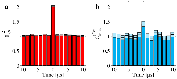
Figure 9: Autocorrelation measurements. a, Autocorrelation measurement for the Stokes field. The histogram has been obtained combining the data corresponding to different Stokes detection probabilities. The measured $g^{(2)}_{s,s}$ value is $2.03(3)$ (see table 1). b, Autocorrelation measurement for the converted anti-Stokes photons. The histogram is obtained combining all the data shown in table 1. The measured $g^{(2)c}_{as,as}$ value is $1.4(1)$.

As we discussed in the previous section, the $\mathrm{SNR}$ depends linearly on the probability to have a photon at the input of the QFCD. When we convert heralded single photons from the QM, this probability is given by the retrieval efficiency $\eta_{R}^{in}$. Since $\eta_{R}^{in}$ is constant over a wide range of Stokes detection probabilities (see Fig. 2 of the main text), for a fixed pump power the $\mathrm{SNR}$ can also be taken as constant in the same $p_{s}$ range. This assumption does not hold for high $p_{s}$ values. However, as we discussed above, in this case equation (8) does not depend on the $\mathrm{SNR}$. Therefore the $\mathrm{SNR}$ can be assumed as constant.

Appendix D Cauchy-Schwarz inequality and autocorrelation measurements

For a pair of independent classical fields, the second order cross-correlation function between the two modes and the relative autocorrelation functions for each mode have to satisfy the following inequality:

$$R=\frac{\left(g^{(2)}_{1,2}\right)^{2}}{g^{(2)}_{1,1}\cdot g^{(2)}_{2,2}}\leq 1,$$ (9)

which constitutes a particular case of the Cauchy-Schwarz inequality Clauser1974 . A violation of the condition expressed by equation (9) indicates that non-classical correlations are present between the two modes. As we explained before, the joint quantum state for the Stokes and anti-Stokes field can be described by the two mode squeezed state defined in equation (4). In the ideal case, the Stokes and the anti-Stokes modes individually display a thermal statistic, i.e. their second order autocorrelation is equal to $2$. Using equation (9), we see that when the cross-correlation function $g^{(2)}_{s,as}$ exceeds the value of $2$, the joint photon statistic shows a quantum behavior. However, for a generic two modes state, the autocorrelation function of each mode can exceed the value of $2$. In this case, it is necessary to achieve higher $g^{(2)}_{s,as}$ values in order to ensure that the Cauchy-Schwarz inequality is violated. For this reason, it is necessary to carefully measure the Stokes and anti-Stokes autocorrelations before assessing the quantum nature of the observed state without assumptions.

In order to measure the Stokes autocorrelation function, we use a $50$-$50$ fiber beam splitter to deliver the photons obtained from our QM to two single photon detectors. The arrival times on the two detectors are measured by means of the time stamping card mentioned above, thus obtaining a coincidence histogram. The $g^{(2)}_{s,s}$ is shown in Fig. 9a. We proceed in a similar way for the anti-Stokes field. The measurements are performed for five different write powers. The results are summarized in the first three columns of table 1, where the two autocorrelation values are listed together with the corresponding measured Stokes detection probabilities. We can observe that the autocorrelation values do not change significantly for the $p_{s}$ range explored in the experiment. For this reason, we can combine all the histograms together and obtain a unique value for the autocorrelations, shown in the last line of the table. The measured $g^{(2)}_{s,s}$ is compatible with the expected thermal statistic. For the anti-Stokes field the observed value is systematically below $2$. This can be explained considering that for the anti-Stokes photons we do not use spectral filtering to further reduce the possible leakage of read light. For this reason the signal to noise ratio is lower in this case. In the fifth column of table 1 we show the value of the Cauchy-Schwarz parameter $R$ calculated from the $g^{(2)}_{s,as}$ measured in the experiment.

Table 1: Values of the Stokes ($g^{(2)}_{s,s}$), anti-Stokes ($g^{(2)}_{as,as}$) and converted anti-Stokes ($g^{(2)c}_{as,as}$) autocorrelation function for various Stokes detection probabilities $p_{s}$. The values shown in the last row are obtained combining all the correlation histograms. In the last two columns the Cauchy-Schwarz parameter $R$ ($R^{c}$) is calculated from the measured $g^{(2)}_{s,as}$ ($g^{(2)c}_{s,as}$) values.

$p_{s}$ [$\%$]	$g^{(2)}_{s,s}$	$g^{(2)}_{as,as}$	$g^{(2)c}_{as,as}$	$R$	$R^{c}$
$1.6$	$2.03(5)$	$1.46(2)$	$1.6(2)$	$12.2(4)$	$4.8(6)$
$1.5$	$2.01(6)$	$1.46(2)$	$1.3(2)$	$12.8(5)$	$6(1)$
$1.0$	$2.03(8)$	$1.41(2)$	$1.4(2)$	$16.4(8)$	$7(1)$
$0.4$	$2.03(5)$	$1.43(4)$	$1.3(2)$	$55(2)$	$21(5)$
	$2.03(3)$	1.45(1)	1.4(1)

It is possible to proceed in a similar way when the atomic based QM is used in combination with the QFCD. For the Stokes field, we can use the same value as before. For the anti-Stokes field, a new measurement is necessary, performed following the same experimental strategy as above (see Fig. 9b). The results are shown in the forth column of table 1, together with their average. The data have been taken using $120\,\mathrm{mW}$ of pump power, measured at the waveguide output. We notice that the measured $g^{(2)c}_{as,as}$ value is below $2$. Similar reasons as before contribute to explain this behavior: the converted anti-Stokes photons are polluted by the broadband noise generated by the strong pump at $1569\,\mathrm{nm}$ while propagating in the non linear waveguide. The integration time used to accumulate the autocorrelation histogram corresponding the lowest $p_{s}$ value reported in table 1 is about $10$ hours. The Cauchy-Schwarz parameter $R^{c}$ shown in the last column is clearly above $1$, thus confirming that the quantum nature of the anti-Stokes photons is preserved in the conversion process.

- (1) Kimble, H. J. The quantum internet. Nature 453, 1023–1030 (2008).
- (2) Hammerer, K., Sørensen, A. S. & Polzik, E. S. Quantum interface between light and atomic ensembles. Rev. Mod. Phys. 82, 1041–1093 (2010).
- (3) Sangouard, N., Simon, C., de Riedmatten, H. & Gisin, N. Quantum repeaters based on atomic ensembles and linear optics. Rev. Mod. Phys. 83, 33–80 (2011).
- (4) Ritter, S. et al. An elementary quantum network of single atoms in optical cavities. Nature 484, 195–200 (2012).
- (5) Moehring, D. L. et al. Entanglement of single-atom quantum bits at a distance. Nature 449, 68–71 (2007).
- (6) Hofmann, J. et al. Heralded entanglement between widely separated atoms. Science 337, 72–75 (2012).
- (7) Chanelière, T. et al. Storage and retrieval of single photons transmitted between remote quantum memories. Nature 438, 833–836 (2005).
- (8) Eisaman, M. D. et al. Electromagnetically induced transparency with tunable single-photon pulses. Nature 438, 837–841 (2005).
- (9) Radnaev, A. G. et al. A quantum memory with telecom-wavelength conversion. Nat Phys 6, 894–899 (2010).
- (10) Hosseini, M., Campbell, G., Sparkes, B. M., Lam, P. K. & Buchler, B. C. Unconditional room-temperature quantum memory. Nat Phys 7, 794–798 (2011).
- (11) Bao, X.-H. et al. Efficient and long-lived quantum memory with cold atoms inside a ring cavity. Nat Phys 8, 517–521 (2012).
- (12) de Riedmatten, H., Afzelius, M., Staudt, M. U., Simon, C. & Gisin, N. A solid-state light-matter interface at the single-photon level. Nature 456, 773–777 (2008).
- (13) Hedges, M. P., Longdell, J. J., Li, Y. & Sellars, M. J. Efficient quantum memory for light. Nature 465, 1052–1056 (2010).
- (14) Clausen, C. et al. Quantum storage of photonic entanglement in a crystal. Nature 469, 508–511 (2011).
- (15) Saglamyurek, E. et al. Broadband waveguide quantum memory for entangled photons. Nature 469, 512–515 (2011).
- (16) Chou, C. W. et al. Functional quantum nodes for entanglement distribution over scalable quantum networks. Science 316, 1316–1320 (2007).
- (17) Yuan, Z.-S. et al. Experimental demonstration of a bdcz quantum repeater node. Nature 454, 1098–1101 (2008).
- (18) Usmani, I. et al. Heralded quantum entanglement between two crystals. Nat Photon 6, 234–237 (2012).
- (19) Briegel, H.-J., Dür, W., Cirac, J. I. & Zoller, P. Quantum repeaters: The role of imperfect local operations in quantum communication. Phys. Rev. Lett. 81, 5932–5935 (1998).
- (20) Duan, L.-M., Lukin, M. D., Cirac, J. I. & Zoller, P. Long-distance quantum communication with atomic ensembles and linear optics. Nature 414, 413–418 (2001).
- (21) Lauritzen, B. et al. Telecommunication-wavelength solid-state memory at the single photon level. Phys. Rev. Lett. 104, 080502– (2010).
- (22) Tanzilli, S. et al. A photonic quantum information interface. Nature 437, 116–120 (2005).
- (23) Rakher, M. T., Ma, L., Slattery, O., Tang, X. & Srinivasan, K. Quantum transduction of telecommunications-band single photons from a quantum dot by frequency upconversion. Nat Photon 4, 786–791 (2010).
- (24) Ates, S. et al. Two-photon interference using background-free quantum frequency conversion of single photons emitted by an inas quantum dot. Phys. Rev. Lett. 109, 147405– (2012).
- (25) Takesue, H. Single-photon frequency down-conversion experiment. Phys. Rev. A 82, 013833– (2010).
- (26) Curtz, N., Thew, R., Simon, C., Gisin, N. & Zbinden, H. Coherent frequency-down-conversion interface for quantum repeaters. Opt. Express 18, 22099–22104 (2010).
- (27) Zaske, S., Lenhard, A. & Becher, C. Efficient frequency downconversion at the single photon level from the red spectral range to the telecommunications c-band. Opt. Express 19, 12825–12836 (2011).
- (28) Zaske, S. et al. Visible-to-telecom quantum frequency conversion of light from a single quantum emitter. Phys. Rev. Lett. 109, 147404– (2012).
- (29) Ikuta, R. et al. Wide-band quantum interface for visible-to-telecommunication wavelength conversion. Nat Commun 2, 537– (2011).
- (30) De Greve, K. et al. Quantum-dot spin-photon entanglement via frequency downconversion to telecom wavelength. Nature 491, 421–425 (2012).
- (31) Felinto, D. et al. Conditional control of the quantum states of remote atomic memories for quantum networking. Nat Phys 2, 844–848 (2006).
- (32) Laurat, J. et al. Efficient retrieval of a single excitation stored in an atomic ensemble. Opt. Express 14, 6912–6918 (2006).
- (33) Fernandez-Gonzalvo, X. et al. Quantum frequency conversion of quantum memory compatible photons to telecommunication wavelengths. Opt. Express 21, 19473–19487 (2013).
- (34) de Riedmatten, H. et al. Direct measurement of decoherence for entanglement between a photon and stored atomic excitation. Phys. Rev. Lett. 97, 113603–4 (2006).
- (35) Sangouard, N. et al. Robust and efficient quantum repeaters with atomic ensembles and linear optics. Phys.Rev.A 77, 062301 (2008).
- (36) Palittapongarnpim, P., MacRae, A. & Lvovsky, A. I. Note: A monolithic filter cavity for experiments in quantum optics. Rev. Sci. Instrum. 83, 066101–3 (2012).
- (37) Mendes, M. S., Saldanha, P. L., Tabosa, J. W. R. & Felinto, D. Dynamics of the reading process of a quantum memory. New Journal of Physics 15, 075030– (2013).
- (38) Kuo, P. S. et al. Reducing noise in single-photon-level frequency conversion. Opt. Lett. 38, 1310–1312 (2013).
- (39) Clauser, J. F. Experimental distinction between the quantum and classical field-theoretic predictions for the photoelectric effect. Phys. Rev. D 9, 853– (1974).