Constraints on exclusive branching fractions $\mathcal{B}_{i}(B^{+}\to X_{c}^{i}l^{+}\nu)$ from moment measurements in inclusive $B\to X_{c}l\nu$ decays

Abstract

As an alternative to direct measurements, we extract exclusive branching fractions of semileptonic $B$-meson decays to charmed mesons, $\mathcal{B}_{i}(B^{+}\to X_{c}^{i}l^{+}\nu)$ with $X_{c}^{i}=D,D^{*},D_{0},D^{\prime}_{1},D_{1},D_{2},D^{\prime},D^{\prime*}$ and non-resonant final states $(D^{(*)}\pi)_{nr}$, from a fit to electron energy, hadronic mass and combined hadronic mass-energy moments measured in inclusive $B\to X_{c}l\nu$ decays. The fit is performed by constraining the sum of exclusive branching fractions to the measured value of $\mathcal{B}(B^{+}\to X_{c}l^{+}\nu)$, and with different sets of additional constraining terms for the directly measured branching fractions. There is no fit scenario in which a single branching fraction alone is enhanced to close the gap between $\mathcal{B}(B^{+}\to X_{c}l^{+}\nu)$ and the sum of known branching fractions $\mathcal{B}_{i}(B^{+}\to X_{c}^{i}l^{+}\nu)$. The fitted $\mathcal{B}(B^{+}\to\overline{D}^{*0}l^{+}\nu)$ is $5\%$ to $10\%$ larger than the direct measurement depending on whether or not $\mathcal{B}(B^{+}\to\overline{D}^{*0}l^{+}\nu)$ is constrained to its direct measurement. $\mathcal{B}(B^{+}\to\overline{D}^{0}l^{+}\nu)$ values are in good agreement with the direct measurement unless $\mathcal{B}(B^{+}\to\overline{D}^{*0}l^{+}\nu)$ is constrained, which results in a higher $\mathcal{B}(B^{+}\to\overline{D}^{0}l^{+}\nu)$ value. Within large uncertainties, $\mathcal{B}(B^{+}\to\overline{D}^{\prime 0}_{1}l^{+}\nu)$ agrees with direct measurements. Depending on the fit scenario, $\mathcal{B}(B^{+}\to\overline{D}^{0}_{0}l^{+}\nu)$ is consistent with or larger than its direct measurement. The fit is not able to easily disentangle $B^{+}\to\overline{D}^{0}_{1}l^{+}\nu$ and $B^{+}\to\overline{D}^{0}_{2}l^{+}\nu$, and tends to increase the sum of these two branching fractions. $\mathcal{B}(B^{+}\to(D^{(*)}\pi)_{nr}l^{+}\nu)$ with non-resonant $(D^{(*)}\pi)_{nr}$ final states is found to be $0.2-0.4\%$, consistent with $B^{+}\to D^{(*)}\pi l^{+}\nu$ and $B^{+}\to\overline{D}^{**}(D^{(*)}\pi)l^{+}\nu$ measurements. No indication is found for significant contributions from so far unmeasured $B^{+}\to\overline{D}^{\prime(*)0}l^{+}\nu$ decays assuming that the $\overline{D}^{\prime 0}$ and $\overline{D}^{\prime*0}$ can be identified with the observed $D(2550)$, respectively, $D^{*}(2600)$ state.

Florian U. Bernlochner
         University of Victoria, Victoria, British Columbia, Canada V8W 3P

Dustin Biedermann
         Humboldt-Universität zu Berlin, 12489 Berlin, Germany

Heiko Lacker
         Humboldt-Universität zu Berlin, 12489 Berlin, Germany

Thomas Lück
         University of Victoria, Victoria, British Columbia, Canada V8W 3P

1 INTRODUCTION

The Cabibbo-Kobayashi-Maskawa (CKM) quark mixing matrix [1] governs the weak coupling strength between up- and down-type quarks. The CKM-matrix element $|V_{cb}|$ can be extracted from semileptonic $B$-meson decays $B\to X_{c}l\nu$ with hadronic final states $X_{c}$ containing mesons with charm whereby inclusive or exclusive final states can be used. For analyses of exclusive final states, such as $B\to D^{(*)}l\nu$ decays, good knowledge about the overall composition of the $X_{c}$ final states is crucial. Precise understanding of semileptonic $B\to X_{c}l\nu$ decays is also of utmost importance for the precision determination of $|V_{ub}|$ from $B\to X_{u}l\nu$ decays, since $B\to X_{c}l\nu$ decays represent the main source of background events in this kind of analyses.
Precise knowledge of $B\to X_{c}l\nu$ decays has also relevance for new physics searches. A ${\displaystyle B}\!{\scriptstyle A}\!{\displaystyle B}\!{\scriptstyle{A\!R}}$  
measurement of $\frac{\mathcal{B}(\overline{B}\to D^{(*)}\tau^{-}\overline{\nu})}{\mathcal{B}(\overline{B}\to D^{(*)}l^{-}\overline{\nu})}$, where $l\in\{e,\mu\}$, exceeds the Standard Model expectations by $3.4\,\sigma$ [2]. In this analysis, an important systematic uncertainty originates from the detailed knowledge of the composition of $B\to D^{**}l\nu$ decays, where $D^{**}$ denotes the four 1P states of non-strange charmed mesons. In particular, $D^{**}$ decays to $D^{(*)}\pi\pi$ states are seen to have a large impact on the measured ratio.

1.1 BRANCHING FRACTION MEASUREMENTS

Great efforts have been made in measuring the inclusive and exclusive branching fractions of $B\to X_{c}l\nu$ transitions. Exclusive branching fractions $\mathcal{B}(B\to X^{i}_{c}l\nu)$ have been determined for the hadronic final states $X_{c}^{i}\in\left\{D,D^{*},D_{0},D^{\prime}_{1},D_{1},D_{2},D^{(*)}\pi\right\}$. Averages for these measurements and for the inclusive branching fraction $\mathcal{B}(B\to X_{c}l\nu)$ are provided by the Heavy Flavor Averaging Group (HFAG) [3], which we use in this paper. In Table 1, we quote all branching fractions for semileptonic decays of charged $B$-mesons, for which measurements exist and which are used in our analysis. Thereby, we assume that the corresponding branching fractions for semileptonic decays of neutral $B$-mesons can be obtained by applying isospin invariance of strong interactions. That is, the decay rates for semileptonic decays of charged and neutral $B$-mesons are set to be equal. The $\mathcal{B}(B^{+}\to\overline{D}^{0}l^{+}\nu)$ and $\mathcal{B}(B^{+}\to\overline{D}^{*0}l^{+}\nu)$ values quoted in Table 1 are calculated from the HFAG (isospin) averages provided for $\mathcal{B}(B^{0}\to D^{(*)-}l^{+}\nu)$ [3] as

$$\mathcal{B}(B^{+}\to\overline{D}^{(*)0}l^{+}\nu)=\tau_{+0}\mathcal{B}(B^{0}\to\overline{D}^{(*)-}l^{+}\nu),$$ (1.1)

with

$$\tau_{+0}:=\frac{\tau_{B^{+}}}{\tau_{B^{0}}}=1.079\pm 0.007$$ (1.2)

being the ratio of lifetimes $\tau_{B^{+}}$ and $\tau_{B^{0}}$ of charged and neutral $B$-mesons, respectively [3]. Since for $\mathcal{B}(B\to X_{c}l\nu)$ quoted in Ref. [3] charged and neutral $B$-meson decays were used, we calculate $\mathcal{B}(B^{+}\to X_{c}l^{+}\nu)$ according to

$$\mathcal{B}(B^{+}\to X_{c}l^{+}\nu)=\tau_{+0}\frac{f_{+0}+1}{1+f_{+0}\tau_{+0}}\mathcal{B}(B\to X_{c}l\nu),$$ (1.3)

with

$$f_{+0}:=\frac{\mathcal{B}(\Upsilon(4S)\to B^{+}B^{-})}{\mathcal{B}(\Upsilon(4S)\to B^{0}\overline{B}^{0})}=1.065\pm 0.026\;$$ (1.4)

being the measured ratio of $\Upsilon(4S)$ branching fractions into charged and neutral $B$-meson pairs as quoted in Ref. [3].
In case of $X^{i}_{c}$ being one of the $D^{\ast\ast}$ mesons $D_{0}$, $D^{\prime}_{1}$, $D_{1}$, or $D_{2}$, only product branching-fractions $\mathcal{B}(B^{+}\to{D}^{\ast\ast}(D^{(*)-}\pi^{+})l^{+}\nu)=\mathcal{B}(B^{+}\to{D}^{\ast\ast}l^{+}\nu)\times\mathcal{B}({D}^{\ast\ast}\to D^{(*)-}\pi^{+})$ are available [3]. In these cases, we have to correct for the branching fraction $\mathcal{B}({D}^{\ast\ast}\to D^{(*)-}\pi^{+})$ to obtain $\mathcal{B}(B^{+}\to{D}^{\ast\ast}l^{+}\nu)$. To do so we assume strong-isospin symmetry. As a result, in case of a $D^{\ast\ast}$ two-body decay, we account for the decay mode of the $D^{\ast\ast}$ in which the created $u$ quark is interchanged by a $d$ quark by introducing a multiplicative factor of $\frac{3}{2}$. Furthermore, we make the following assumptions: the $D_{0}$ can only decay into $D\pi$, the $D^{\prime}_{1}$ only into $D^{*}\pi$, the $D_{1}$-meson only into $D^{*}\pi$ and $D\pi\pi$, and the $D_{2}$-meson into $D\pi$ and $D^{*}\pi$.

In cases of $D_{1}$ decays we use the average of measurements for the ratio (see Appendix B)

$$\begin{split}\frac{\mathcal{B}(B^{+}\to\overline{D}_{1}^{0}(D\pi\pi)\pi^{+})}{\mathcal{B}(B^{+}\to\overline{D}_{1}^{0}(D^{*}\pi)\pi^{+})}=0.53\pm 0.14,\end{split}$$ (1.5)

relying on Refs. [4, 5, 6, 7], and obtain $\mathcal{B}(B^{+}\to\overline{D}^{0}_{1}l^{+}\nu)$ according to

$$\begin{split}\mathcal{B}(B^{+}\to\overline{D}_{1}^{0}l^{+}\nu)=\left(1+\frac{\mathcal{B}(B^{+}\to\overline{D}_{1}^{0}(D\pi\pi)\pi^{+})}{\mathcal{B}(B^{+}\to\overline{D}_{1}^{0}(D^{*}\pi)\pi^{+})}\right)\times\mathcal{B}(B^{+}\to\overline{D}_{1}^{0}(D^{*}\pi)l^{+}\nu).\end{split}$$ (1.6)

For the $D_{2}$-meson we use the measured ratio [8]

$$\frac{\mathcal{B}(D_{2}^{0}\to D^{+}\pi^{-})}{\mathcal{B}(D_{2}^{0}\to D^{*+}\pi^{-})}=1.56\pm 0.16,$$ (1.7)

and calculate $\mathcal{B}(B^{+}\to\overline{D}_{2}^{0}l^{+}\nu)$ in an analogous way as $\mathcal{B}(B^{+}\to\overline{D}_{1}^{0}l^{+}\nu)$.
Measurements for $B^{+}\to D^{(*)}\pi l^{+}\nu$ have been performed as well. Using the HFAG averages of these branching fractions [3] together with the $\mathcal{B}(B^{+}\to\overline{D}^{\ast\ast}(D^{(*)}\pi)l^{+}\nu)$ averages [3] we determine the branching fraction for semileptonic decays into non-resonant ($nr$) final states $(D^{(*)}\pi)_{nr}$. For these cases, we calculate the isospin average according to equation C.1 as described in Appendix C.
The values for $\mathcal{B}(B^{+}\to X^{i}_{c}l^{+}\nu)$, with $X_{c}^{i}$ being $D_{0}$, $D^{\prime}_{1}$, $D_{1}$, $D_{2}$, and $(D^{(*)}\pi)_{nr}$, obtained in this way, are quoted in Table 1.

1.2 PUZZLES AND POSSIBLE SOLUTIONS

Some serious problems arise from the quoted branching fractions:

• The most obvious puzzle and in the following denoted as ”gap problem” results from the fact that the sum of the directly measured exclusive branching fractions does not saturate the measured inclusive branching fraction, i.e.

  $$\begin{split}\mathcal{B}(B^{+}\to X_{c}l^{+}\nu)=(10.90\pm 0.14)\%\neq\sum\limits_{i=D,D^{*},D^{**}}\mathcal{B}_{i}(B^{+}\to X_{c}^{i}l^{+}\nu)=(9.2\pm 0.2)\%.\end{split}$$ (1.8)

  Even if the branching fraction for decays into non-resonant $(D^{(*)}\pi)_{nr}$, $\mathcal{B}(B^{+}\to(D^{(*)}\pi)_{nr}l^{+}\nu)$, is taken into consideration as well, the gap can not be closed.

• A more subtle problem and commonly referred to as the ”$\frac{1}{2}$ vs. $\frac{3}{2}$ puzzle” [9] concerns the sector of $B\to D^{**}l\nu$ decays. Theoretical deliberations [9, 10, 11] suggest that the branching fraction of $B\to D_{1}/D_{2}l\nu$ decays should be about one order of magnitude larger than $\mathcal{B}(B\to D_{0}/D^{\prime}_{1}l\nu)$. The measured values are in clear contradiction to this expectation.
  It should be noted though that a quark-model based calculation essentially agrees with the measured values of all $B\to D^{**}l\nu$ transitions [12]. If correct this would be in contrast to the stated ”$\frac{1}{2}$ vs. $\frac{3}{2}$ puzzle” [9, 10, 11].

• Furthermore, the branching fraction of $B^{+}\to\overline{D}^{\prime 0}_{1}l^{+}\nu$ decays which is given in Table 1 is the result of a weighted average of three measurements from DELPHI [13], Belle [14] and ${\displaystyle B}\!{\scriptstyle A}\!{\displaystyle B}\!{\scriptstyle{A\!R}}$   [15]:

  • $\mathcal{B}(B^{+}\to\overline{D}^{\prime 0}_{1}(D^{*-}\pi^{+})l^{+}\nu)=(0.74\pm 0.17\pm 0.18)\%$ (DELPHI),

  • $\mathcal{B}(B^{+}\to\overline{D}^{\prime 0}_{1}(D^{*-}\pi^{+})l^{+}\nu)=(-0.03\pm 0.06\pm 0.07)\%$ (Belle),

  • $\mathcal{B}(B^{+}\to\overline{D}^{\prime 0}_{1}(D^{*-}\pi^{+})l^{+}\nu)=(0.27\pm 0.04\pm 0.04)\%$ (${\displaystyle B}\!{\scriptstyle A}\!{\displaystyle B}\!{\scriptstyle{A\!R}}$  ).

  When averaging these three measurements one obtains a $\chi^{2}$ over degrees of freedom ($dof$) of $\chi^{2}/dof=\frac{18}{2}$ corresponding to a confidence level of $0.1\%$. Possibly, at least one measurement underestimates the uncertainty, thus the average might be biased and the uncertainty on the weighted average might be underestimated.

Decay	Branching Fraction [%]
$B^{+}\to\overline{D}^{0}l^{+}\nu$	$2.30\pm 0.10$
$B^{+}\to\overline{D}^{*0}l^{+}\nu$	$5.34\pm 0.12$
$B^{+}\to\overline{D}_{1}^{0}l^{+}\nu$	$0.652\pm 0.071$
$B^{+}\to\overline{D}_{2}^{0}l^{+}\nu$	$0.284\pm 0.032$
$B^{+}\to\overline{D}_{1}^{\prime 0}l^{+}\nu$	$0.195\pm 0.060$
$B^{+}\to\overline{D}_{0}^{0}l^{+}\nu$	$0.435\pm 0.075$
$B^{+}\to(D^{(*)}\pi)_{nr}l^{+}\nu$	$0.17\pm 0.14$
$B^{+}\to X_{c}l^{+}\nu$	$10.90\pm 0.14$

Table 1: Semileptonic branching fractions $\mathcal{B}(B^{+}\to X^{(i)}_{c}l^{+}\nu)$ taken or calculated from HFAG averages [3] as described in the text.

Possible experimental issues that might be the source for these puzzles are:

• Exclusive decay channels $B\to X_{c}^{i}l\nu$ into final states $X_{c}^{i}$ not measured yet could contribute significantly to the inclusive semileptonic decay rate. Such transitions could be for example $B\to D^{\prime(*)}l\nu$, where $D^{\prime(*)}$ might be the recently discovered resonances $D(2550)$ and $D^{*}(2600)$ [16]. In Ref. [17] a rough estimation suggested that a combined branching fraction of about $1\%$ could be realized in nature for $B\to D^{\prime(*)}l\nu$ whereas in Ref. [18] it was argued that such a large branching fraction would be difficult to understand theoretically.

• It is possible that not all $D^{**}$ decay channels were incorporated when determining $\mathcal{B}(B\to D_{1}/D_{2}l\nu)$ from the measured product branching fractions. For example, there might be $D_{1}\to D^{*}\pi\pi$, $D_{2}\to D^{*}\pi\pi$ (upper limits are given in Ref. [4]), $D_{1}/D_{2}\to D_{0}/D^{\prime}_{1}\pi$ and $D_{2}\to D\eta$ decays with sizeable branching fractions [19]. If true this would relax both the ”gap problem” and the ”$\frac{1}{2}$ vs. $\frac{3}{2}$ puzzle” at the same time.

• Another possibility would be that the branching fraction of $B\to D^{(*)}l\nu$ decays is experimentally underestimated, which would ease the ”gap problem” but not the ”$\frac{1}{2}$ vs. $\frac{3}{2}$ puzzle”. However, $\mathcal{B}(B\to D^{(*)}l\nu)$ is measured with high precision. As a consequence, one would need to enlarge these branching fractions signifcantly more than it is allowed by the quoted uncertainty in order to relax the ”gap problem”.
  One possible effect that could lead to a biased estimate of the $B\to D^{*}l\nu$ branching fraction is an overestimate of the reconstruction efficiency of the low-energy pion appearing in the $D^{*}$ decay to a $D$ and a $\pi$. It should be noted though that the experimental measurement that has a very strong weight in the average extracts $\mathcal{B}(B\to D^{*}l\nu)$ from a global fit to kinematical distributions without relying on the reconstruction of the low-energy pion from the $D^{*}$ decay [20].
  If there is no experimental problem with the reconstruction of the low-energy pions or other issues relevant to the analyses, another explanation of underestimated $B\to D^{(*)}l\nu$ branching fractions could be overestimated $D$ and/or $D^{*}$ branching fractions. However, $D$-meson branching fractions are very well determined by experiments running on the $\psi(3770)$ resonance, such as CLEO-c or BES-III. Since the $\psi(3770)$ decays into $D\overline{D}$, absolute branching-fraction measurements are possible by tagging one $D$-meson and measuring the decay of the other one into a specific final state.
  For the $D^{*}$-meson, possible electromagnetic decays not measured yet are $D^{*}\to De^{+}e^{-}$ and $D^{*}\to D\gamma\gamma$. These decays would have to compete at least with $D^{*}\to D\gamma$ in order to have a sizeable effect on $\mathcal{B}(B\to D^{*}l\nu)$. This would come as a real surprise since one would expect a rate suppression of these decays of the order the fine-structure constant $\alpha\approx 1/137$ with respect to $D^{*}\to D\gamma$.

• Reconstructing $B\to D^{\prime}_{1}l\nu$ and $B\to D_{0}l\nu$ with $D_{0}/D^{\prime}_{1}\to D^{*}\pi$ is not an easy experimental task as the $D_{0}$ and the $D_{1}^{\prime}$ are very broad resonances and therefore hard to distinguish from non-resonant $(D^{(*)}\pi)_{nr}$ final states. Therefore, the correct values for $\mathcal{B}(B\to D^{\prime}_{1}l\nu)$ and $\mathcal{B}(B\to D_{0}l\nu)$ could be indeed smaller than the HFAG averages, which would relax the ”$\frac{1}{2}$ vs. $\frac{3}{2}$ puzzle”, but not the ”gap problem”.

• Non-resonant decays $B\to(D^{(*)}\pi)_{nr}l\nu$ could fill the gap. If this is true, this would suggest a serious problem in the $B\to D^{(*)}\pi l\nu$ and/or $B\to D^{**}(D^{(*)}\pi)l\nu$ analysis since the $B\to D^{(*)}\pi l\nu$ together with the $B\to D^{**}(D^{(*)}\pi)l\nu$ results leave only a small space for $B\to(D^{(*)}\pi)_{nr}l\nu$ decays. In addition, theoretical expectations do not support a large branching fraction for non-resonant $B\to(D^{(*)}\pi)_{nr}l\nu$ decays [17].

• There might be contributions from yet to be discovered $B\to(D^{(*)}\pi\pi)_{nr}l\nu$ or $B\to(D^{(*)}\eta)_{nr}l\nu$ decays, which would ease the ”gap problem”. Such decays have not been observed yet and we did not investigate them in our analysis since our general findings do not prefer large contributions from high-mass states like $B\to D^{\prime(*)}l\nu$ or from non-resonant decays $B\to(D^{(*)}\pi)_{nr}l\nu$ so that we don’t expect significant contributions from $B\to(D^{(*)}\pi\pi)_{nr}l\nu$ or $B\to(D^{(*)}\eta)_{nr}l\nu$ decays either. Moreover, by adding too many free parameters to the problem our analysis would loose in sensitivity.

Kinematical distributions of the lepton energy $E_{l}$ and the hadronic invariant mass $m_{X_{c}}$ measured in inclusive $B\to X_{c}l\nu$ decays are sensitive to the composition of exclusive final states containing mesons with charm. Usually, moments of these kinematical distributions are used to extract non-perturbative parameters of a Heavy Quark Expansion (HQE) [21, 22, 23, 24, 25, 26] with the aim to measure the CKM matrix element $\left|V_{cb}\right|$ (e.g. Ref. [27]) with highest precision. In this paper, we make use of such moment measurements to fit exclusive branching fractions $\mathcal{B}(B^{+}\to X_{c}^{i}l^{+}\nu)$ with the aim to shed additional light on a solution to the puzzles described above. We investigate the contributions to the inclusive branching fraction from exclusive final states $X_{c}^{i}=D$, $D^{*}$, $D_{0}$, $D^{\prime}_{1}$, $D_{1}$, $D_{2}$, $(D^{(*)}\pi)_{nr}$, and $D^{\prime(*)}$. Hereby, we assume that $\overline{D}^{\prime 0}$ and $\overline{D}^{\prime*0}$ can be identified with the observed $D(2550)$, respectively, $D^{*}(2600)$ state. One should stress that a moment of a kinematical distribution for any specific exclusive decay $B\to X_{c}^{i}l\nu$, with $X_{c}^{i}$ being a resonant state such as $D$, $D^{*}$, $D_{0}$, $D^{\prime}_{1}$, $D_{1}$, $D_{2}$ , or $D^{\prime(*)}$, does not depend on the branching fractions of such a resonance decaying into specific final states. Therefore, branching-fraction values found by the fit being larger than the directly measured values may indicate that the $X_{c}^{i}$ decay branching-fractions assumed are overestimated.

In Section 2, we describe the moments entering our analysis as fit inputs. Section 3 provides information concerning the Monte-Carlo events used for the calculation of the moments for an exclusive decay. In Section 4, we outline the fit procedure and its validation, and we present the fit results in Section 5. In the last section we give a summary.

2 MOMENTS IN SEMILEPTONIC DECAYS

For our analysis we use three different kinds of moments: moments of the electron-energy spectrum, of the hadronic mass spectrum and of the combined hadronic energy-mass spectrum, which were measured at the experiments ${\displaystyle B}\!{\scriptstyle A}\!{\displaystyle B}\!{\scriptstyle{A\!R}}$   [27], Belle [28, 29], CLEO [30], and DELPHI [31]. In Table 2, we quote the moment measurements to which we fit the branching fractions.
In the following, moments which correspond to a single decay mode we refer to as ”exclusive moments”, while when summing over exclusive decay modes we refer to the term ”inclusive moments”.
We calculate the theoretical prediction for these moments from Monte-Carlo (MC) simulated events using the following estimators, where the nomenclature is based on Ref. [27]:

• The estimator for the first electron-energy moment $M_{1}$ is given by
  

  $$M_{1}\left(E_{cut_{0}}\right)=\left\langle E\right\rangle_{E_{cut_{0}}}=\frac{\sum\limits^{E_{i}>E_{cut_{0}}}_{i}{g_{i}E_{i}}}{\sum\limits^{E_{i}>E_{cut_{0}}}_{i}{g_{i}}},$$ (2.1)

  where $E_{cut_{0}}$ is the lower electron-energy cut-off above which the electron energies are included in the calculation of the moment and $E_{i}$ is the energy of the electron of the $i$-th event in the $B$-meson rest frame. To switch between different form-factor models in exclusive decays we introduce the event weights $g_{i}$.
  For higher moments, the estimator is given by

  $$\begin{split}M_{k}\left(E_{cut_{0}}\right)=\left\langle\left(E-\left\langle E\right\rangle_{E_{cut_{0}}}\right)^{k}\right\rangle=\frac{\sum\limits^{E_{i}>E_{cut_{0}}}_{i}{g_{i}\left(E_{i}-\left<E\right>_{E_{cut_{0}}}\right)^{k}}}{\sum\limits^{E_{i}>E_{cut_{0}}}_{i}{g_{i}}},\end{split}$$ (2.2)

  with $k>1$.
  For later convenience, the exclusive and inclusive moments are arranged in vectors:

  $$\begin{split}\vec{M}=\left({\begin{array}[]{*{20}c}{M_{1}\left(E_{cut_{0}}\right)}\\ {M_{1}\left(E_{cut_{1}}\right)}\\ \vdots\\ {M_{2}\left(E_{cut_{0}}\right)}\\ {M_{2}\left(E_{cut_{1}}\right)}\\ \vdots\\ {M_{3}\left(E_{cut_{0}}\right)}\\ {M_{3}\left(E_{cut_{1}}\right)}\\ \vdots\\ \end{array}}\right)=\left({\begin{array}[]{*{20}c}{\left\langle{E}\right\rangle_{E_{cut_{0}}}}\\ {\left\langle{E}\right\rangle_{E_{cut_{1}}}}\\ \vdots\\ {\left\langle{\left({E-\left\langle{E}\right\rangle}\right)^{2}}\right\rangle_{E_{cut_{0}}}}\\ {\left\langle{\left({E-\left\langle{E}\right\rangle}\right)^{2}}\right\rangle_{E_{cut_{1}}}}\\ \vdots\\ {\left\langle{\left({E-\left\langle{E}\right\rangle}\right)^{3}}\right\rangle_{E_{cut_{0}}}}\\ {\left\langle{\left({E-\left\langle{E}\right\rangle}\right)^{3}}\right\rangle_{E_{cut_{1}}}}\\ \vdots\\ \end{array}}\right).\\ \end{split}$$ (2.3)

  Here, $E_{cut_{i}}$ denotes again the corresponding lower electron-energy cut-off.
  We define in addition the vector

  $$\begin{split}\left<\vec{E}\right>=\left({\begin{array}[]{*{20}c}{\left<E\right>_{E_{cut_{0}}}}\\ {\left<E\right>_{E_{cut_{1}}}}\\ \vdots\\ {\left<E^{2}\right>_{E_{cut_{0}}}}\\ {\left<E^{2}\right>_{E_{cut_{1}}}}\\ \vdots\\ {\left<E^{3}\right>_{E_{cut_{0}}}}\\ {\left<E^{3}\right>_{E_{cut_{1}}}}\\ \vdots\\ \end{array}}\right).\\ \end{split}$$ (2.4)

• The non-central moments of the hadronic mass spectrum in $B\to X_{c}l\nu$ decays are defined as the mean of powers of the invariant hadronic mass. Again they are measured as a function of a lower lepton ($e$ or $\mu$) momentum cut-off $p_{cut_{0}}$ in the $B$-meson rest frame.
  The estimators of the mass moments are given by:

  $$\left\langle m^{k}\right\rangle_{p_{cut_{0}}}=\frac{\sum\limits^{p_{i}>p_{cut_{0}}}_{i}{g_{i}m^{k}_{X_{i}}}}{\sum\limits^{p_{i}>p_{cut_{0}}}_{i}{g_{i}}},$$ (2.5)

  with $m_{X_{i}}$ being the invariant hadronic mass of event $i$.
  The estimator of the central mass moments are defined as

  $$\left\langle m^{2}_{centr}\right\rangle_{p_{cut_{0}}}=\frac{\sum\limits^{p_{i}>p_{cut_{0}}}_{i}{g_{i}\left(m_{X_{i}}^{2}-\bar{M}_{D}^{2}\right)}}{\sum\limits^{p_{i}>p_{cut_{0}}}_{i}{g_{i}}},$$ (2.6)

  as well as

  $$\left\langle m^{4}_{centr}\right\rangle_{p_{cut_{0}}}=\frac{\sum\limits^{p_{i}>p_{cut_{0}}}_{i}{g_{i}\left(m_{X_{i}}^{2}-\bar{M}_{D}^{2}\right)^{2}}}{\sum\limits^{p_{i}>p_{cut_{0}}}_{i}{g_{i}}}.$$ (2.7)

  Here, $i$ runs over all events for which $p_{i}>p_{cut_{0}}$, where $p_{i}$ is the lepton momentum in the semileptonic decay, $p_{cut_{0}}$ the cut-off momentum, $g_{i}$ the event weight and $\bar{M}_{D}=\left(m_{D}+3m_{D^{*}}\right)/4=1.973\rm\,{GeV/c^{2}}$, with $m_{D}$ and $m_{D^{*}}$ the masses of the $D$ meson and $D^{*}$ meson, respectively.
  Again, these moments are written in form of a vector:

  $$\begin{split}\left\langle\vec{m}\right\rangle=\left({\begin{array}[]{*{20}c}{\left\langle{m}\right\rangle_{p_{cut_{0}}}}\\ {\left\langle{m}\right\rangle_{p_{cut_{1}}}}\\ \vdots\\ {\left\langle{m^{2}}\right\rangle_{p_{cut_{0}}}}\\ {\left\langle{m^{2}}\right\rangle_{p_{cut_{1}}}}\\ \vdots\\ {\left\langle{m^{3}}\right\rangle_{p_{cut_{0}}}}\\ {\left\langle{m^{3}}\right\rangle_{p_{cut_{1}}}}\\ \vdots\\ \end{array}}\right),\end{split}$$ (2.8)

  whereby the vector of central moments with respect to $\bar{M}^{2}_{D}$ is defined analogously

  $$\begin{split}\left\langle\vec{m}\right\rangle_{centr}=\left({\begin{array}[]{*{20}c}{\left\langle{m^{2}_{centr}}\right\rangle_{p_{cut_{0}}}}\\ {\left\langle{m^{2}_{centr}}\right\rangle_{p_{cut_{1}}}}\\ \vdots\\ {\left\langle{m^{4}_{centr}}\right\rangle_{p_{cut_{0}}}}\\ {\left\langle{m^{4}_{centr}}\right\rangle_{p_{cut_{1}}}}\\ \vdots\\ \end{array}}\right).\end{split}$$ (2.9)

• In Ref. [32] a measurement of combined mass-energy moments was proposed. These moments are for instance better controlled theoretically and therefore they may result in a more reliable extraction of higher-order non-pertubative HQE parameters. Hence, a more accurate determination of the Standard Model parameters $|V_{cb}|$, the charm quark mass $m_{c}$ and the bottom quark mass $m_{b}$ should be possible. The first three even combined mass-energy moments were measured by the ${\displaystyle B}\!{\scriptstyle A}\!{\displaystyle B}\!{\scriptstyle{A\!R}}$  collaboration [27]. Here, we use the following estimators for the prediction of these moments:

  $$\begin{split}\left\langle n^{k}\right\rangle_{p_{cut_{0}}}=\frac{1}{\sum\limits^{p_{i}>p_{cut_{0}}}_{i}{g_{i}}}\sum\limits^{p_{i}>p_{cut_{0}}}_{i}{g_{i}\left(m_{X_{i}}^{2}c^{4}-2\tilde{\Lambda}E_{X_{i}}+\tilde{\Lambda}^{2}\right)^{k/2}},\end{split}$$ (2.10)

  where $i$ runs over all events for which $p_{i}>p_{cut_{0}}$, $E_{X_{i}}$ denotes the hadronic energy and $m_{X_{i}}$ the invariant mass of the hadronic system $X_{i}$, $p_{i}$ is the momentum of the involved lepton measured in the $B$-meson rest frame, $p_{cut_{0}}$ is the lower momentum cut-off, $g_{i}$ is again the corresponding event weight, and $\tilde{\Lambda}=0.65\,\rm{GeV}$ [32].
  These moments are also arranged in a vector:

  $$\begin{split}\left\langle\vec{n}\right\rangle=\left({\begin{array}[]{*{20}c}{\left\langle{n^{2}}\right\rangle_{p_{cut_{0}}}}\\ {\left\langle{n^{2}}\right\rangle_{p_{cut_{1}}}}\\ \vdots\\ {\left\langle{n^{4}}\right\rangle_{p_{cut_{0}}}}\\ {\left\langle{n^{4}}\right\rangle_{p_{cut_{1}}}}\\ \vdots\\ {\left\langle{n^{6}}\right\rangle_{p_{cut_{0}}}}\\ {\left\langle{n^{6}}\right\rangle_{p_{cut_{1}}}}\\ \vdots\\ \end{array}}\right).\\ \end{split}$$ (2.11)

In Table 2, we quote the moments measured at a specific lower cut-off which are used in the fit procedure. Since the measurements were unfolded for efficiency and detector resolution effects they can be directly compared with theoretical calculations.
Moments with lower cut-offs $E_{cut}$ or $p_{cut}$ close to each other are highly correlated and can result in numerical problems such as non-positive-definiteness of the final covariance matrices. As a consequence, we select data from a subset of available lower cut-offs to avoid these problems.

	Exp.	$E_{cut}[\rm{GeV}]$ or $p_{cut}[\rm{GeV/c}]$	Ref.
$M_{1}$	${\displaystyle B}\!{\scriptstyle A}\!{\displaystyle B}\!{\scriptstyle{A\!R}}$	0.6, 0.8, 1.0, 1.2, 1.5	[27]
$M_{2}$	${\displaystyle B}\!{\scriptstyle A}\!{\displaystyle B}\!{\scriptstyle{A\!R}}$	0.6, 0.8, 1.0, 1.2, 1.5	[27]
$M_{3}$	${\displaystyle B}\!{\scriptstyle A}\!{\displaystyle B}\!{\scriptstyle{A\!R}}$	0.6, 0.8, 1.0, 1.2, 1.5	[27]
$\left\langle m^{1}\right\rangle$	${\displaystyle B}\!{\scriptstyle A}\!{\displaystyle B}\!{\scriptstyle{A\!R}}$	1.1, 1.3, 1.5, 1.7, 1.9	[27]
$\left\langle m^{2}\right\rangle$	${\displaystyle B}\!{\scriptstyle A}\!{\displaystyle B}\!{\scriptstyle{A\!R}}$	0.8, 1.2, 1.4, 1.6, 1.8	[27]
$\left\langle m^{3}\right\rangle$	${\displaystyle B}\!{\scriptstyle A}\!{\displaystyle B}\!{\scriptstyle{A\!R}}$	0.9, 1.1, 1.5, 1.7, 1.9	[27]
$\left\langle m^{4}\right\rangle$	${\displaystyle B}\!{\scriptstyle A}\!{\displaystyle B}\!{\scriptstyle{A\!R}}$	0.8, 1.0, 1.2, 1.6, 1.8	[27]
$\left\langle m^{5}\right\rangle$	${\displaystyle B}\!{\scriptstyle A}\!{\displaystyle B}\!{\scriptstyle{A\!R}}$	0.9, 1.1, 1.3, 1.5, 1.9	[27]
$\left\langle m^{6}\right\rangle$	${\displaystyle B}\!{\scriptstyle A}\!{\displaystyle B}\!{\scriptstyle{A\!R}}$	0.8, 1.0, 1.2, 1.4, 1.6	[27]
$\left\langle n^{2}\right\rangle$	${\displaystyle B}\!{\scriptstyle A}\!{\displaystyle B}\!{\scriptstyle{A\!R}}$	0.8 - 1.9, in steps of 0.1	[27]
$\left\langle n^{4}\right\rangle$	${\displaystyle B}\!{\scriptstyle A}\!{\displaystyle B}\!{\scriptstyle{A\!R}}$	0.8 - 1.9, in steps of 0.1	[27]
$\left\langle n^{6}\right\rangle$	${\displaystyle B}\!{\scriptstyle A}\!{\displaystyle B}\!{\scriptstyle{A\!R}}$	0.8 - 1.9, in steps of 0.1	[27]
$M_{1}$	Belle	1.0, 1.4	[28]
$M_{2}$	Belle	0.6, 1.4	[28]
$M_{3}$	Belle	0.8, 1.2	[28]
$M_{4}$	Belle	0.6, 1.2	[28]
$\left\langle m^{2}\right\rangle$	Belle	0.7 - 1.9, in steps of 0.2	[29]
$\left\langle m^{4}\right\rangle$	Belle	0.7 - 1.9, in steps of 0.2	[29]
$\left\langle m^{2}_{centr}\right\rangle$	CLEO	1.0, 1.5	[30]
$\left\langle m^{4}_{centr}\right\rangle$	CLEO	1.0, 1.5	[30]
$M_{1}$	DELPHI	0.0	[31]
$M_{2}$	DELPHI	0.0	[31]
$M_{3}$	DELPHI	0.0	[31]

Table 2: Experimentally measured moments used to constrain exclusive semileptonic branching fractions in $B\to X_{c}l\nu$ decays.

3 MODELLING OF $B\to X_{c}^{i}l\nu$ DECAYS

For the calculation of the exclusive moments we use for every mode $5\cdot 10^{6}$ MC events generated with the EvtGen event generator [33]. After the generation we use the XslFF reweighting package [34] to reweight the events according to more up-to-date form-factor models:

• $B\to Dl\nu$ decays are modeled according to the Heavy Quark Effective Theory (HQET) model with the Caprini-Lellouch-Neubert (CLN) parametrization [36].

• $B\to D^{*}l\nu$ are modeled according to the HQET model with the CLN parametrization [36].

• $B\to D^{**}l\nu$ decays are modeled according to approximation B1 of the Leibovich-Ligeti-Stewart-Wise (LLSW) model [37].

• $B\to(D^{(*)}\pi)_{nr}l\nu$ decays are modeled according to the Goity-Roberts model [38].

• $B\to D^{\prime(*)}l\nu$ decays are modeled according to the Bernlochner-Ligeti-Turczyk (BLT) model [17]. Here, we assume that the $2S$ states $D^{\prime}$ and $D^{\prime*}$ can be identified with the observed resonances $D(2550)$ and $D^{*}(2600)$ [16] and accordingly assign the masses and widths to the measured values given in Ref. [16]:

  • $m(D^{\prime 0})=2.5394\,\rm{GeV/c^{2}}$, $\Gamma(D^{\prime 0})=130\,\rm{MeV}$

  • $m(D^{\prime\pm})=2.5394\,\rm{GeV/c^{2}}$, $\Gamma(D^{\prime\pm})=130\,\rm{MeV}$

  • $m(D^{\prime*0})=2.6087\,\rm{GeV/c^{2}}$, $\Gamma(D^{\prime*0})=93\,\rm{MeV}$

  • $m(D^{\prime*\pm})=2.6213\,\rm{GeV/c^{2}}$, $\Gamma(D^{\prime*\pm})=93\,\rm{MeV}$

  assuming $m(D(2550)^{0})=m(D(2550)^{\pm})$, $\Gamma(D(2550)^{0})=\Gamma(D(2550)^{\pm})$.

The parameters for the CLN model are taken from Ref. [3] and were obtained by a global fit to all available $\mathcal{B}(B\to D^{*}l\nu)$ measurements:

• $\rho^{2}_{A_{1}}(1)=1.207\pm 0.026$,

• $R_{1}(1)=1.403\pm 0.033$,

• $R_{2}(1)=0.854\pm 0.020$,

with associated correlation coefficients:

• $\rho_{\rho^{2},R1}=0.566$

• $\rho_{\rho^{2},R2}=-0.807$

• $\rho_{R1,R2}=-0.759$

The parameter for the LLSW model is set to (see Ref. [37])

• $\hat{\tau}^{\prime}=-1.5\pm 0.5$

with the estimated uncertainty taken from Ref. [37].
The BLT parameters are chosen to be equal to (see Ref. [17])

• $\beta_{0}=0.13$, $\beta_{1}=1.95\pm 0.05$, $\beta_{2}=-7.0\pm 1.3$

• $\beta^{*}_{0}=0.1$, $\beta^{*}_{1}=2.4\pm 0.1$, $\beta^{*}_{2}=-6.65\pm 3.15$

with estimated uncertainties taken from Ref. [17].
The non-resonant decays $B\to(D^{(*)}\pi)_{nr}l\nu$ (with $l\in\{e,\mu\}$) are a mixture of several channels which is experimentally unknown (see Appendix C). Since Ref. [38] suggests that the mixture is dominated by $B\to(D\pi)_{nr}l\nu$ transitions, we choose the following composition:

• $B^{0}\to(D^{*-}\pi^{0})_{nr}l^{-}\overline{\nu}:8.6\%$

• $B^{0}\to(\overline{D}^{*0}\pi^{-})_{nr}l^{-}\overline{\nu}:17.3\%$

• $B^{0}\to(D^{-}\pi^{0})_{nr}l^{-}\overline{\nu}:24.7\%$

• $B^{0}\to(\overline{D}^{0}\pi^{-})_{nr}l^{-}\overline{\nu}:49.4\%$

and analogously for $\overline{B}^{0}$ decays.
Non-resonant $B^{+}$ decays are composed as follows:

• $B^{+}\to(D^{*-}\pi^{+})_{nr}l^{+}\nu:15.4\%$

• $B^{+}\to(\overline{D}^{*0}\pi^{0})_{nr}l^{+}\nu:7.7\%$

• $B^{+}\to(D^{-}\pi^{+})_{nr}l^{+}\nu:51.3\%$

• $B^{+}\to(\overline{D}^{0}\pi^{0})_{nr}l^{+}\nu:25.6\%$

and analogously for $B^{-}$ decays.

4 MOMENT FITTER

We perform a $\chi^{2}-fit$ to the mentioned moments, taking the full covariance of each moment vector into account.

4.1 $\chi^{2}$-FUNCTION

To estimate the semileptonic branching fractions in $B\to X_{c}^{i}l\nu$ decays from moment measurements we minimize the following $\chi^{2}$-function using the MINUIT package [39]:

$$\chi^{2}=\sum\limits_{j}{\left(\chi^{2}_{\rm{n},j}+\chi^{2}_{\rm{M},j}+\chi^{2}_{\rm{m},j}\right)}+\chi_{\rm{sum}}^{2}+\chi^{2}_{\rm{constr}},$$ (4.1)

with

$$\begin{split}\chi^{2}_{\rm{n},j}&=\left({\vec{\left\langle{n}\right\rangle}\left(\mathcal{B}^{i}\right)-\vec{\left\langle{n}\right\rangle}_{exp}^{j}}\right)^{T}C_{\rm{n},j}^{-1}\left({\vec{\left\langle{n}\right\rangle}\left(\mathcal{B}^{i}\right)-\vec{\left\langle{n}\right\rangle}_{exp}^{j}}\right),\\ \chi^{2}_{\rm{M},j}&=\left({\vec{{M}}\left(\mathcal{B}^{i}\right)-\vec{{M}}_{exp}^{j}}\right)^{T}C_{\rm{M},j}^{-1}\left({\vec{{M}}\left(\mathcal{B}^{i}\right)-\vec{{M}}_{exp}^{j}}\right),\\ \chi^{2}_{\rm{m},j}&=\left({\vec{\left\langle{m}\right\rangle}\left(\mathcal{B}^{i}\right)-\vec{\left\langle{m}\right\rangle}_{exp}^{j}}\right)^{T}C_{\rm{m},j}^{-1}\left({\vec{\left\langle{m}\right\rangle}\left(\mathcal{B}^{i}\right)-\vec{\left\langle{m}\right\rangle}_{exp}^{j}}\right),\end{split}$$ (4.2)

where the index $j$ runs over the different moment measurements, $C_{\rm{n},j}$, $C_{\rm{M},j}$ and $C_{\rm{m},j}$ are the sums of the related experimental and theoretical covariance matrices and the different theoretical moments are functions of the current values of the set of the fitted $N$ branching fractions $\mathcal{B}^{i}:=\mathcal{B}^{i}_{fit}(B^{+}\to X_{c}^{i}l^{+}\nu)$, $i=1,\ldots,N$. The experimentally measured moment vectors are denoted with a subscript ”exp”.
It is assumed that there is no correlation between the moment vectors $\left\langle\vec{n}\right\rangle$, $\vec{M}$ and $\left\langle\vec{m}\right\rangle$ for both, experimentally measured and theoretically predicted. In case of ${\displaystyle B}\!{\scriptstyle A}\!{\displaystyle B}\!{\scriptstyle{A\!R}}$  , electron moments were measured by leptonically tagging the other $B$-meson decay by a leptonic tag whereas mass and combined mass-energy moments were measured by fully reconstructing the other $B$-meson decay. Therefore, we consider the electron moments measured by ${\displaystyle B}\!{\scriptstyle A}\!{\displaystyle B}\!{\scriptstyle{A\!R}}$  as being uncorrelated with the other moments. In case of the Belle measurements, the electron moments have been measured on the recoil of fully reconstructed $B$-meson decays. In this case, there are correlations with the hadronic moments measured by Belle which, however, we neglect in the fit since the uncertainties on the electron moments are smaller for the ${\displaystyle B}\!{\scriptstyle A}\!{\displaystyle B}\!{\scriptstyle{A\!R}}$  measurements.
The experimental correlation between the combined mass-energy moments $\left\langle n^{k}\right\rangle$, which were only measured by ${\displaystyle B}\!{\scriptstyle A}\!{\displaystyle B}\!{\scriptstyle{A\!R}}$  , and the mass moments $\left\langle m^{l}\right\rangle$ measured by ${\displaystyle B}\!{\scriptstyle A}\!{\displaystyle B}\!{\scriptstyle{A\!R}}$   is a-priori not negligible. Unfortunately, Ref. [41] provides only a subset of the correlation coefficients and therefore the full set of correlations for these moments can not be included in the fit. Since the complete correlation matrix is missing, we decided to omit the correlations between $\left\langle n^{k}\right\rangle$ and $\left\langle m^{l}\right\rangle$ for the ${\displaystyle B}\!{\scriptstyle A}\!{\displaystyle B}\!{\scriptstyle{A\!R}}$   measurements and studied how the fit result changes when assigning a correlation matrix which uses the partial information quoted in Ref. [41] (see Section 4.2).
In case of the theoretical prediction, the electron, the combined mass-energy and mass moments are statistically correlated. However, since the experimental covariances are dominant, we neglect these correlations.
The sum of the fitted branching fractions is always constrained to the inclusive branching fraction by adding

$$\chi_{sum}^{2}=\frac{\left(\mathcal{B}_{exp}(B^{+}\to X_{c}l^{+}\nu)-\sum\limits_{i}\mathcal{B}^{i}\right)^{2}}{\sigma^{2}_{exp}},$$ (4.3)

where $\mathcal{B}_{exp}(B^{+}\to X_{c}l^{+}\nu)$ and its uncertainty $\sigma_{exp}$ are given in the last line of Table 1.
The number of degrees of freedom of the fit can be increased by using additional constraints for those branching fractions which are experimentally known from direct measurements as listed in Table 1. This is achieved by adding the optional term:

$$\chi^{2}_{constr}=\sum\limits_{j}{\frac{\left(\mathcal{B}^{j}_{exp}(B^{+}\to X_{c}^{j}l^{+}\nu)-\mathcal{B}^{j}\right)^{2}}{\sigma^{2}_{exp,j}}},$$ (4.4)

where $\mathcal{B}^{j}_{exp}(B\to X_{c}^{j}l\nu)$ are the values of those particular semileptonic branching fractions that are externally constrained with $\sigma_{exp,j}$ being their corresponding experimental uncertainties.

From the exclusive moments the inclusive moments are predicted by the sum of exclusive moments with coefficients proportional to the corresponding exclusive branching fractions.
Since the moment measurements get contributions from charged and neutral $B$-meson decays, we decompose the predicted moments into contributions from both. In this composition, we assume equal semileptonic decay rates of charged and neutral $B$-meson decays as a consequence of strong-isospin symmetry resulting in

$$\mathcal{B}(B^{+}\to X_{c}^{i}l^{+}\nu)=\tau_{+0}\mathcal{B}(B^{0}\to X_{c}^{i}l^{+}\nu).$$ (4.5)

For any inclusive moment $\left\langle Z^{k}\right\rangle$ (except for central moments) with a lower leptonic energy or momentum cut-off ”cut”, one can write then

$$\begin{split}\left\langle Z^{k}\right\rangle_{cut}=\frac{\sum\limits_{t}^{N_{m}/2}{\mathcal{B}_{t}\left(\frac{f_{+0}}{1+f_{+0}}\frac{N_{cut}^{t}}{N_{t}}\left\langle Z^{k}\right\rangle_{cut}^{t}+\frac{1}{\tau_{+0}}\frac{1}{1+f_{+0}}\frac{N_{cut}^{\tilde{t}}}{N_{\tilde{t}}}\left\langle Z^{k}\right\rangle_{cut}^{\tilde{t}}\right)}+\mathcal{B}_{nr}\frac{N_{cut}^{nr}}{N_{nr}}\left\langle Z^{k}\right\rangle_{cut}^{nr}}{\sum\limits_{t}^{N_{m}/2}{\mathcal{B}_{t}\left(\frac{f_{+0}}{1+f_{+0}}\frac{N_{cut}^{t}}{N_{t}}+\frac{1}{\tau_{+0}}\frac{1}{1+f_{+0}}\frac{N_{cut}^{\tilde{t}}}{N_{\tilde{t}}}\right)}+\mathcal{B}_{nr}\frac{N_{cut}^{nr}}{N_{nr}}}\end{split}$$ (4.6)

Here, $N_{m}$ denotes the number of exclusive decay modes of charged and neutral $B$-mesons included in the fit, $N_{t}$ corresponds to the number of events of decay mode $t$ of a charged $B$-meson, $N^{t}_{cut}$ is the number of events of decay mode $t$ passing the cut-off, $\tilde{t}$ denotes the decay mode of a neutral $B$-meson that is isospin-symmetrical to the decay mode $t$, and $\left\langle Z^{k}\right\rangle^{t}_{cut}$ is the exclusive moment of mode $t$ measured at a cut-off ”cut”. We add the contribution of the non-resonant decays differently compared to the other decay channels, since the moments of the non-resonant decays were already calculated from a mixture of charged and neutral $B$-meson decays.

The central moment vector $\vec{Z}_{centr}$ is computed by a linear transformation from their non-central equivalents $\vec{Z}$ as $\vec{Z}_{centr}=J\vec{Z}$ with $J$ being the Jacobian of the transformation $\vec{Z}\to\vec{Z}_{centr}$.

The theoretical inclusive covariance matrices are calculated from the set of theoretical exclusive covariance matrices. The inclusive moment vector $\left\langle\vec{Z}\right\rangle$ can be written as

$${\left\langle{\vec{Z}}\right\rangle}=\left({\begin{array}[]{*{20}c}{\frac{{\sum\limits_{t}{b^{t}_{cut_{1}}\left\langle{Z}\right\rangle^{t}_{cut_{1}}}}}{{\sum\limits_{t}{b^{t}_{cut_{1}}}}}}\\ {\frac{{\sum\limits_{t}{b^{t}_{cut_{2}}\left\langle{Z}\right\rangle^{t}_{cut_{2}}}}}{{\sum\limits_{t}{b^{t}_{cut_{2}}}}}}\\ \vdots\\ {\frac{{\sum\limits_{t}{b^{t}_{cut_{n}}\left\langle{Z}\right\rangle^{t}_{cut_{n}}}}}{{\sum\limits_{t}{b^{t}_{cut_{n}}}}}}\\ \end{array}}\right),$$ (4.7)

where $t$ runs over all incorporated decay modes of charged and neutral $B$-mesons, $b^{t}_{cut_{i}}=\tilde{f}_{t}\mathcal{B}_{t}\frac{N^{t}_{cut_{i}}}{N_{t}}$, $cut_{i}$ denotes either a lower lepton energy or momentum cut-off and $\tilde{f}_{t}$ either equals $\frac{f_{+0}}{1+f_{+0}}$ if $t$ corresponds to a decay mode of a charged $B$-meson or $\frac{1}{\tau_{+0}\left(1+f_{+0}\right)}$ if $t$ corresponds to a decay mode of a neutral $B$-meson.
$\vec{Z}$ can be rewritten as a sum of products of exclusive moment vectors $\left<\vec{Z}\right>_{t}$ and transformation matrices $F_{t}$:

$$\begin{split}\left\langle{\vec{Z}}\right\rangle&=\sum\limits_{t}{diag\left(\frac{b^{t}_{cut_{1}}}{{\sum\limits_{t}{b^{t}_{cut_{1}}}}},\frac{b^{t}_{cut_{2}}}{{\sum\limits_{t}{b^{t}_{cut_{2}}}}},\cdots,\frac{b^{t}_{cut_{n}}}{{\sum\limits_{t}{b^{t}_{cut_{n}}}}}\right){\left\langle{\vec{Z}}\right\rangle_{t}}}\\ &=\sum\limits_{t}{F_{t}{\left\langle{\vec{Z}}\right\rangle_{t}}}.\end{split}$$ (4.8)

As a result, the covariance matrix of an inclusive moment vector is given by

$$\begin{split}C_{\left\langle\vec{Z}\right\rangle}=\sum_{t}{F_{t}C_{\left\langle\vec{Z}\right\rangle_{t}}F^{T}_{t}}.\end{split}$$ (4.9)

We approximate the theoretical covariance matrix of a central moment vector by

$$C_{\langle\vec{Z}_{centr}\rangle}=JC_{\langle\vec{Z}\rangle}J^{T},$$ (4.10)

with the Jacobian $J$ of the transformation $\vec{Z}\to\vec{Z}_{centr}$.

4.2 STATISTICAL AND SYSTEMATIC COVARIANCES

• The computation of the statistical covariances is described in detail in Appendix A

• Within our fit model one systematic arises from the choice of the form-factor parameters. To obtain an estimate for these systematics, the calculation of theoretical moments is performed with randomly varied form-factor parameters. The variation is made by adding Gaussian random numbers to the nominal values of the form-factor parameters, whereby we account for the measured correlations of the parameters $\rho^{2}_{A_{1}}(1)$, $R_{1}(1)$ and $R_{2}(1)$ in the case of $B^{+}\to\overline{D}^{*0}l^{+}\nu$. The central values are chosen to be zero and the Gaussian standard deviations are chosen to be the parameter uncertainties as quoted in Section 3.
  The variations of all form factors are performed 100 times and afterwards the systematic covariances of the obtained moment vectors are calculated for each mode, according to
  $C_{\left\langle\vec{Z}\right\rangle}=\left\langle\left(\left\langle\vec{Z}\right\rangle-\overline{\left\langle\vec{Z}\right\rangle}\right)\left(\left\langle\vec{Z}\right\rangle-\overline{\left\langle\vec{Z}\right\rangle}\right)^{T}\right\rangle$, where $\vec{Z}$ is the respective moment vector.

• As mentioned in Section 4.1 the full correlation matrix between mass and combined mass-energy moments is missing. To investigate the influence of the omitted correlations we assume that the correlation matrix between $\left\langle n^{2}\right\rangle$ and $\left\langle m^{2}\right\rangle$, which is quoted in Ref. [41], holds between all $\left\langle n^{k}\right\rangle$ and $\left\langle m^{l}\right\rangle$, which should overestimate the correlations. When performing the fits with these correlations, the fit results change typically only by about $10\%$ and in rare cases up to $40\%$ with respect to the associated fit uncertainty. The uncertainties themselves change by about $10\%$. Therefore, the qualitative picture does not change and we conclude that neglecting the correlations between mass and mass-energy moments are of minor importance.

• The sensitivity of the fit with respect to the modeling of $B\to(D^{(*)}\pi)_{nr}l\nu$ decays is checked by varying the mixture of $(D\pi)_{nr}$ and $(D^{*}\pi)_{nr}$ final states: For the extreme case that only $B\to(D\pi)_{nr}l\nu$ is simulated to predict the moments for $B\to(D^{(*)}\pi)_{nr}l\nu$, none of the fit results for any branching fraction changes more than $20\%$ with respect to the associated fit error. For the case that only $B\to(D^{*}\pi)_{nr}l\nu$ is simulated to predict the moments for
  $B\to(D^{(*)}\pi)_{nr}l\nu$, the situation becomes more involved. In this case, there are some scenarios in which the results for $D^{\ast\ast}$ and $(D^{*}\pi)_{nr}$ change more than $100\%$ with respect to the fit uncertainty. While Ref. [38] suggests a clear dominance of $B\to(D\pi)_{nr}l\nu$ decays over $B\to(D^{*}\pi)_{nr}l\nu$ decays, the experimental constraints do not exclude the contrary (see Appendix C). Therefore, we provide in Appendix I the results for our considered fit scenarios in which $B\to(D^{(*)}\pi)_{nr}l\nu$ decays are modeled exclusively with $B\to(D^{*}\pi)_{nr}l\nu$ decays.

• The widths of the broad $D^{**}$ mesons are only known with an uncertainty of about $30\%$. By varying their widths in the fit we study the influence on the fit result. Most of the branching fractions are - compared to the corresponding fit uncertainty - quite insensitive to this variation. Only ${\mathcal{B}}(B^{+}\to\overline{D}^{0}_{1}l^{+}\nu)$ and ${\mathcal{B}}(B^{+}\to\overline{D}^{\prime 0}_{1}l^{+}\nu)$ show some sensitivity. But even in these case their fit values do not change more than $O(50\%)$ compared to their associated fit uncertainties. Hence, our qualitative findings are not modified by this effect.

4.3 FIT VALIDATION

No change of the fit results is observed when the initial values of the branching fractions $\mathcal{B}(B^{+}\to X^{i}_{c}l^{+}\nu)$ are chosen arbitrarily in the interval [0,$\mathcal{B}(B^{+}\to X_{c}l^{+}\nu)$].
To check for a potential bias of the fit results and the calculated uncertainties, the fit is tested with a ”statistical ensemble of pseudo-experiments”. This ”pseudo-data” is obtained from a statistical variation of a particular mixture of the exclusive moments according to the experimental covariance matrix $C_{exp}$ as follows:
Nominal inclusive moment vectors $\left<\vec{Z}_{i}\right>_{0}$ ($i$ runs over the different used moment vectors) calculated according to the measured set of values of the branching fractions $\{\mathcal{B}^{nom}_{i}\}$ are chosen. Then, random vectors $\vec{x}=L\vec{z}$ are added, where $L$ is defined by $C_{exp}=LL^{T}$ and $\vec{z}$ is a standard normal distributed random vector. Since the theoretical exclusive moment vectors are also only known within statistical uncertainties due to the limited Monte-Carlo statistics, they are varied in an analogous way.
From the set of ensemble fits normalized residuals (as defined in the Appendix E) and p-value distributions are obtained. We performed the fit on 1000 pseudo data sets for each fit scenario in Section 5. A typical example of residuals and p-value distributions can be found in Appendix E.
Some small fit bias is observed. Compared to the fit uncertainty the bias for the individual branching fractions found is: $5\%$ or smaller for $\mathcal{B}(B^{+}\to\overline{D}^{0}l^{+}\nu)$, $7\%$ or smaller for $\mathcal{B}(B^{+}\to\overline{D}^{*0}l^{+}\nu)$, up to $25\%$ but typically of order $10\%$ for the narrow-width $D^{**}$, $6\%$ or smaller for the broad-width $D^{**}$, and $5\%$ or smaller for $(D^{(*)}\pi)_{nr}$. Depending on the decay also a small underestimation of the fit uncertainty is observed. Compared to the true uncertainty the underestimation for the individual branching fractions found is: $7\%$ or smaller for $\mathcal{B}(B^{+}\to\overline{D}^{0}l^{+}\nu)$, no significant underestimation for $\mathcal{B}(B^{+}\to\overline{D}^{*0}l^{+}\nu)$, $15\%$ or less for the narrow-width $D^{**}$, $10\%$ or less for the broad-width $D^{**}$, and $8\%$ or smaller for $(D^{(*)}\pi)_{nr}$.
The observed p-value distributions are not perfectly uniform, typically with a mean of $0.56\pm 0.01$ and a RMS of $0.29\pm 0.01$. This small deviation from a uniform distribution is caused by approximating the covariance of the theoretical inclusive central moments with Eq. 4.10. If the central moments are not included in the fit, the p-value distribution gets uniform and the (small) intrinsic bias as well as the (slight) underestimation of the uncertainties observed in the residuals is significantly reduced.

5 RESULTS

$X_{c}$	Fit 1		Fit 2		Fit 3		Fit 4		Measured
	U/C	$\mathcal{B}[\%]$	U/C	$\mathcal{B}[\%]$	U/C	$\mathcal{B}[\%]$	U/C	$\mathcal{B}[\%]$	$\mathcal{B}[\%]$
$\overline{D}^{0}$	x/-	$2.43\pm 0.15$	x/-	$2.43\pm 0.15$	x/-	$2.37\pm 0.15$	x/-	$2.61\pm 0.14$	$2.30\pm 0.10$
$\overline{D}^{*0}$	x/-	$5.81\pm 0.16$	x/-	$5.86\pm 0.16$	x/-	$5.89\pm 0.16$	x/x	$5.53\pm 0.09$	$5.34\pm 0.12$
$\overline{D}_{1}^{0}$	x/-	$2.13\pm 0.67$	x/-	$1.33\pm 0.33$	x/x	$0.67\pm 0.07$	x/-	$1.34\pm 0.33$	$0.65\pm 0.07$
$\overline{D}_{2}^{0}$	x/-	$-0.52\pm 0.59$	x/x	$0.28\pm 0.03$	x/-	$0.61\pm 0.29$	x/x	$0.28\pm 0.03$	$0.28\pm 0.03$
$\overline{D}^{\prime 0}_{1}$	x/-	$0.21\pm 0.34$	x/-	$0.02\pm 0.31$	x/-	$0.19\pm 0.34$	x/-	$0.19\pm 0.30$	$0.20\pm 0.06$
$\overline{D}_{0}^{0}$	x/-	$0.48\pm 0.33$	x/-	$0.60\pm 0.32$	x/-	$0.93\pm 0.26$	x/-	$0.55\pm 0.31$	$0.43\pm 0.07$
$\overline{D}^{\prime 0}$	-/-	-	-/-	-	-/-	-	-/-	-	-
$\overline{D}^{\prime*0}$	-/-	-	-/-	-	-/-	-	-/-	-	-
$(D^{(*)}\pi)_{nr}$	x/-	$0.36\pm 0.16$	x/-	$0.37\pm 0.16$	x/-	$0.25\pm 0.15$	x/-	$0.27\pm 0.16$	-
$\overline{D}^{0}_{1}/\overline{D}^{0}_{2}$	$1.61\pm 0.33$		$1.61\pm 0.33$		$1.28\pm 0.29$		$1.62\pm 0.32$		$0.94\pm 0.08$
$\overline{D}^{0}_{0}/\overline{D}^{\prime 0}_{1}$	$0.69\pm 0.54$		$0.62\pm 0.53$		$1.12\pm 0.50$		$0.73\pm 0.52$		$0.63\pm 0.10$
$\overline{D}^{0}_{0}/\overline{D}^{\prime 0}_{1}/(D^{(*)}\pi)_{nr}$	$1.06\pm 0.40$		$0.99\pm 0.39$		$1.37\pm 0.37$		$1.00\pm 0.39$		$0.63\pm 0.10$
$\sum_{i}X_{c}^{i}$	$10.90\pm 0.14$		$10.90\pm 0.14$		$10.90\pm 0.14$		$10.77\pm 0.13$		$9.21\pm 0.20$
$X_{c}$									$10.90\pm 0.14$
$\chi^{2}/dof$	75/104 = 0.73		77/105 = 0.74		80/105 = 0.77		84/106 = 0.80		-
p-value	0.98		0.98		0.96		0.94		-

Table 3: Results for fits with moments of semileptonic decays with hadronic final states containing $D$, $D^{*}$, any $D^{**}$ or $(D^{(*)}\pi)_{nr}$. Hereby, “U/C” stands for “used/constrained” and the “x” denotes “yes”, whereas “-” denotes “no”, respectively. This table is further discussed and described in the text of Section 5.

$X_{c}$	Fit 5		Fit 6		Fit 7		Fit 8		Measured
	U/C	$\mathcal{B}[\%]$	U/C	$\mathcal{B}[\%]$	U/C	$\mathcal{B}[\%]$	U/C	$\mathcal{B}[\%]$	$\mathcal{B}[\%]$
$\overline{D}^{0}$	x/x	$2.41\pm 0.08$	x/x	$2.44\pm 0.08$	x/x	$2.42\pm 0.08$	x/-	$2.61\pm 0.14$	$2.30\pm 0.10$
$\overline{D}^{*0}$	x/x	$5.59\pm 0.09$	x/x	$5.60\pm 0.09$	x/x	$5.63\pm 0.09$	x/x	$5.51\pm 0.10$	$5.34\pm 0.12$
$\overline{D}_{1}^{0}$	x/-	$1.10\pm 0.30$	x/-	$1.38\pm 0.18$	x/x	$0.78\pm 0.07$	x/-	$1.42\pm 0.33$	$0.65\pm 0.07$
$\overline{D}_{2}^{0}$	x/x	$0.28\pm 0.03$	x/x	$0.28\pm 0.03$	x/x	$0.30\pm 0.03$	x/x	$0.28\pm 0.03$	$0.28\pm 0.03$
$\overline{D}^{\prime 0}_{1}$	x/-	$0.32\pm 0.29$	x/-	$0.19\pm 0.27$	x/x	$0.22\pm 0.06$	x/-	$0.54\pm 0.39$	$0.20\pm 0.06$
$\overline{D}_{0}^{0}$	x/-	$0.78\pm 0.29$	x/x	$0.46\pm 0.07$	x/x	$0.56\pm 0.07$	x/-	$0.54\pm 0.31$	$0.43\pm 0.07$
$\overline{D}^{\prime 0}$	-/-	-	-/-	-	x/-	$0.35\pm 0.12$	x/-	$-0.32\pm 0.22$	-
$\overline{D}^{\prime*0}$	-/-	-	-/-	-	-/-	-	-/-	-	-
$(D^{(*)}\pi)_{nr}$	x/-	$0.20\pm 0.15$	x/-	$0.31\pm 0.11$	x/-	$0.31\pm 0.07$	x/-	$0.21\pm 0.16$	-
$\overline{D}^{0}_{1}/\overline{D}^{0}_{2}$	$1.38\pm 0.30$		$1.66\pm 0.17$		$1.08\pm 0.07$		$1.70\pm 0.33$		$0.94\pm 0.08$
$\overline{D}^{0}_{0}/\overline{D}^{\prime 0}_{1}$	$1.10\pm 0.49$		$0.64\pm 0.29$		$0.78\pm 0.09$		$1.07\pm 0.58$		$0.63\pm 0.10$
$\overline{D}^{0}_{0}/\overline{D}^{\prime 0}_{1}/(D^{(*)}\pi)_{nr}$	$1.30\pm 0.36$		$0.96\pm 0.20$		$1.09\pm 0.10$		$1.28\pm 0.44$		$0.63\pm 0.10$
$\sum_{i}X_{c}^{i}$	$10.68\pm 0.12$		$10.65\pm 0.12$		$10.56\pm 0.12$		$10.78\pm 0.13$		$9.21\pm 0.20$
$X_{c}$									$10.90\pm 0.14$
$\chi^{2}/dof$	88/107 = 0.82		89/108 = 0.83		110/109 = 1.01		82/105 = 0.79		-
p-value	0.91		0.90		0.45		0.94		-

Table 4: Results for fits with moments of semileptonic decays with hadronic final states containing $D$, $D^{*}$, any $D^{**}$ or $(D^{(*)}\pi)_{nr}$. Hereby, “U/C” stands for “used/constrained” and the “x” denotes “yes”, whereas “-” denotes “no”, respectively. This table is further discussed and described in the text of Section 5.

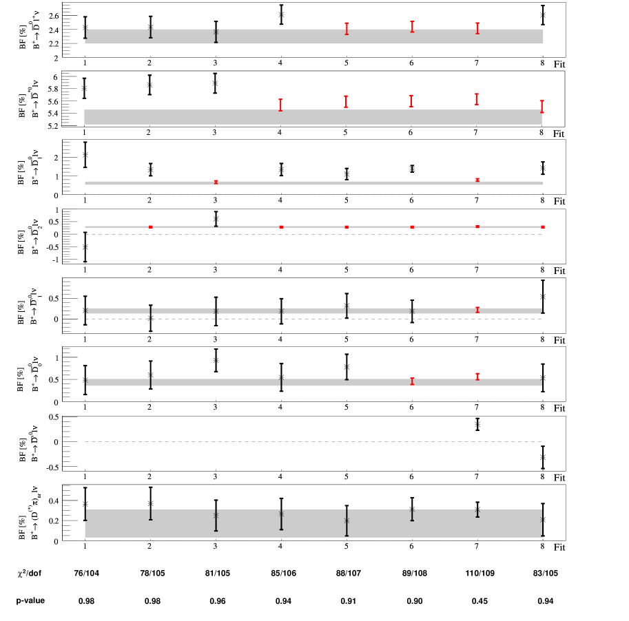
Figure 1: Depiction of the fit results as quoted in Tables 3 and 4. In each subplot the abscissa indicates a distinctive fit scenario labeled by a number, whereas the ordinate represents the branching fraction. The results for a constrained branching fraction are depicted as red points, whereas the results for a unconstrained branching fraction are depicted as a black star. The grey bands correspond to the particular one-sigma error band of the direct branching-fraction measurements. If the ordinate includes zero, a dashed black line visualizes the zero line.

The results of a representative set of fits are quoted in Tables 3 and 4 and are plotted in Fig. 1. We provide further fit results in Appendix F and the related plots in Appendix G. In the result tables, every fit result is presented as a column, consisting of an upper part, which is split into two subcolumns, and a lower part. The upper part provides in its left subcolumn the informations about the fit constellation. The “x” or “-” on the lefthand side denotes whether the moments of this special decay mode are used (“U”) in the fit or not, whereas the “x” or “-” on the righthand side denotes whether this particular branching fraction was or was not constrained (“C”) by a $\chi^{2}_{constr}$ term (as described in Section 4). In addition to the individual branching fraction results, also the sums $\mathcal{B}(B^{+}\to\overline{D}^{0}_{1}l^{+}\nu)+\mathcal{B}(B^{+}\to\overline{D}^{0}_{2}l^{+}\nu)$ and $\mathcal{B}(B^{+}\to\overline{D}^{0}_{0}l^{+}\nu)+\mathcal{B}(B^{+}\to\overline{D}^{\prime 0}_{1}l^{+}\nu)$ as well as $\mathcal{B}(B^{+}\to\overline{D}^{0}_{0}l^{+}\nu)+\mathcal{B}(B^{+}\to\overline{D}^{\prime 0}_{1}l^{+}\nu)+\mathcal{B}(B^{+}\to(D^{*}\pi)_{nr}l^{+}\nu)$ are quoted in order to see whether the “$\frac{1}{2}$ vs. $\frac{3}{2}$ puzzle” is relaxed within a given fit scenario. Finally, the sum of all fitted branching fractions and its uncertainty taking into account the correlations between the fitted $\mathcal{B}_{i}(B^{+}\to X_{c}^{i}l^{+}\nu)$ is compared with the inclusive $\mathcal{B}(B^{+}\to X_{c}l^{+}\nu)$. The lower part quotes the $\chi^{2}$ together with the number of degrees of freedom ($dof$) and the corresponding p-value. In the last column, the directly measured values are quoted for comparison.
The plot in Fig. 1 is composed of several subplots, where each row presents the result of a particular branching fraction. The abscissa labels a certain fit scenario with a number. In addition, the error band (grey band) of the direct measurement and the zero line (dashed black line) are visualized. Those branching fractions that are treated as a fit parameter can be deduced directly from the given plots, because only for branching fractions used in the fit results are plotted. If a branching fraction is constrained in the fit by a $\chi^{2}_{constr}$ term the fit result is plotted as a red point. Otherwise, if the branching fraction is free to vary, the fit result is visualized by a black star. At the bottom of the plots we quote the $\chi^{2}$ value, the number of degrees of freedom and the associated p-value for each fit scenario.
For one of the fits (fit 2 of Table 3) we show in Appendix D how the fit result compares with the measured moments.

In general, none of the scenarios we have studied could be really excluded by the moment fit. However, it should be stressed that the initial $\chi^{2}/dof$ using the measured branching fractions as given in Table 1 ($\mathcal{B}(B\to(D^{(*)}\pi)_{nr}l\nu)$ is set to zero) is found to be $\chi^{2}/dof=394/112=3.6$ (p-value: $5\cdot 10^{-33}$) with a constraint applied for the sum of the branching fractions. Without this constraint we find for the initial $\chi^{2}/dof=248/111=2.2$ (p-value: $1.8\cdot 10^{-12}$). That is, the inclusively measured moments are not well described by the exclusive moments calculated from the measured branching fractions. As a consequence, solving simultaneously the gap problem and the poor description of the inclusive moments requires enhancing certain branching fractions compared to others or adding yet unmeasured exclusive semileptonic decays or both.
A general finding of our analysis is that not a single decay mode alone is capable of filling the gap and better describing the inclusive moments, but that always a set of branching fractions is increased by the fit.
We did not apply a constraint in the fit that forces the branching fractions to be positive in order to avoid fit biases for branching fractions that are close to zero. For fit scenarios in which one of the branching fractions is found to be significantly negative we find that this branching fraction is highly anti-correlated to another one. In such cases, the fit rather constrains the sum of two particular branching fractions than both individually. For this reason, we consider fit scenarios in which one of such two branching fractions is constrained to its directly measured value as being more robust and more meaningful.

• Fit without any constraint on exclusive branching fractions:
  In the first fit scenario, we apply no additional constraint and include those decays in the fit which are known to contribute to $B^{+}\to X_{c}l^{+}\nu$.
  In this first fit scenario, $\mathcal{B}(B^{+}\to\overline{D}^{0}_{2}l^{+}\nu)$ is fitted to a negative value, whereas $\mathcal{B}(B^{+}\to\overline{D}^{0}_{1}l^{+}\nu)$ is extremely large. This is due to a large anti-correlation between these two branching fractions as discussed above. The correlation matrix for the result vector

  $$\begin{split}\vec{\mathcal{B}}=\left({\begin{array}[]{*{20}c}{\mathcal{B}(B^{+}\to\overline{D}^{0}l^{+}\nu)}\\ {\mathcal{B}(B^{+}\to\overline{D}^{*0}l^{+}\nu)}\\ {\mathcal{B}(B^{+}\to\overline{D}^{0}_{1}l^{+}\nu)}\\ {\mathcal{B}(B^{+}\to\overline{D}^{0}_{2}l^{+}\nu)}\\ {\mathcal{B}(B^{+}\to\overline{D}^{\prime 0}_{1}l^{+}\nu)}\\ {\mathcal{B}(B^{+}\to\overline{D}^{0}_{0}l^{+}\nu)}\\ {\mathcal{B}(B^{+}\to(D^{(*)}\pi)_{nr}l^{+}\nu)}\\ \end{array}}\right)\\ \end{split}$$ (5.1)

  of Fit 1 quoted in Table 3 is

  $$\begin{split}\left({\begin{array}[]{*{20}c}1&-0.54&0.19&0.03&-0.16&-0.45&0.13\\ -0.54&1&-0.21&0.24&-0.33&0.13&0.32\\ 0.19&-0.21&1&-0.87&0.01&-0.63&0.34\\ 0.03&0.24&-0.87&1&-0.40&0.26&0.03\\ -0.16&-0.33&0.01&-0.40&1&0.28&-0.79\\ -0.45&0.13&-0.63&0.26&0.28&1&-0.62\\ 0.13&0.32&0.34&0.03&-0.79&-0.62&1\\ \end{array}}\right).\end{split}$$ (5.2)

  showing the large negative correlation coefficient of $-0.87$ between ${\mathcal{B}(B^{+}\to\overline{D}^{0}_{1}l^{+}\nu)}$ and
  ${\mathcal{B}(B^{+}\to\overline{D}^{0}_{2}l^{+}\nu)}$. As a consequence, the fit is not able to clearly distinguish between these two modes and, therefore, it is more meaningful to always either constrain one of these branching fractions to the directly measured value or even fix one of them at zero and always consider only the combination of the two.
  

• Constraints on $\mathcal{B}(B^{+}\to\overline{D}^{0}_{2}l^{+}\nu)$ or $\mathcal{B}(B^{+}\to\overline{D}^{0}_{1}l^{+}\nu)$:
  In Fit 2, we constrain $\mathcal{B}(B^{+}\to\overline{D}^{0}_{2}l^{+}\nu)$ to its measured value.
  Taking into account additional, similar fit scenarios as quoted in Appendix F, we find a combined branching fraction into narrow $D^{**}$ mesons of about $1.3\%$ to $1.7\%$ with uncertainties varying between $0.18\%$ and $0.33\%$. These fit results are clearly above the sum of the directly measured branching fractions:
  $\mathcal{B}(B^{+}\to\overline{D}^{0}_{1}l^{+}\nu)+\mathcal{B}(B^{+}\to\overline{D}^{0}_{2}l^{+}\nu)=\left(0.94\pm 0.08\right)\%$.
  The increase in $\mathcal{B}(B^{+}\to\overline{D}^{0}_{1}l^{+}\nu)+\mathcal{B}(B^{+}\to\overline{D}^{0}_{2}l^{+}\nu)$ points to a possible solution of the “$\frac{1}{2}$ vs. $\frac{3}{2}$ puzzle”: $\mathcal{B}(B^{+}\to\overline{D}^{0}_{0}l^{+}\nu)$ and $\mathcal{B}(B^{+}\to\overline{D}^{\prime 0}_{1}l^{+}\nu)$ are both in very good agreement with the directly measured values quoted in Table 1. As a consequence, the ratio $(\mathcal{B}(B^{+}\to\overline{D}^{0}_{1}l^{+}\nu)+\mathcal{B}(B^{+}\to\overline{D}^{0}_{2}l^{+}\nu))/(\mathcal{B}(B^{+}\to\overline{D}^{0}_{0}l^{+}\nu)+\mathcal{B}(B^{+}\to\overline{D}^{\prime 0}_{1}l^{+}\nu))$ is increased in all fit scenarios where $\mathcal{B}(B^{+}\to\overline{D}^{0}_{2}l^{+}\nu)$ is constrained by a $\chi^{2}_{\rm{constr}}$ term.
  However, if $\mathcal{B}(B^{+}\to\overline{D}^{0}_{1}l^{+}\nu)$ is constrained instead of $\mathcal{B}(B^{+}\to\overline{D}^{0}_{2}l^{+}\nu)$, the findings are bit different (see fit scenario 3). In this case, not only $\mathcal{B}(B^{+}\to\overline{D}^{0}_{2}l^{+}\nu)$ is increased, which is expected due to the large anticorrelation with $\mathcal{B}(B^{+}\to\overline{D}^{0}_{1}l^{+}\nu)$, but also $\mathcal{B}(B^{+}\to\overline{D}^{0}_{0}l^{+}\nu)$. As a result, $(\mathcal{B}(B^{+}\to\overline{D}^{0}_{1}l^{+}\nu)+\mathcal{B}(B^{+}\to\overline{D}^{0}_{2}l^{+}\nu))/(\mathcal{B}(B^{+}\to\overline{D}^{0}_{0}l^{+}\nu)+\mathcal{B}(B^{+}\to\overline{D}^{\prime 0}_{1}l^{+}\nu))$ is of order one and the “$\frac{1}{2}$ vs. $\frac{3}{2}$ puzzle” would be even more pronounced. This is a general finding in all fits where $\mathcal{B}(B^{+}\to\overline{D}^{0}_{1}l^{+}\nu)$ is constrained instead of $\mathcal{B}(B^{+}\to\overline{D}^{0}_{2}l^{+}\nu)$. It turns out that the moment fits in which $\mathcal{B}(B^{+}\to\overline{D}^{0}_{2}l^{+}\nu)$ are constrained instead of $\mathcal{B}(B^{+}\to\overline{D}^{0}_{1}l^{+}\nu)$ result in slightly better p-values as can be seen in Appendix F although the difference between the two fit scenarios is small.
  We note that one could have used lower bounds for the branching fractions into states containing a narrow $D^{**}$ instead of constraining them directly to its measured value since only product branching-fractions are directly measured. We have tested this option and find that either the fit results do not change compared to the case when constraining the branching fraction (in case of Fit 2) or reproduce another already covered fit scenario (Fit 3 would reproduce the result of Fit 1 without any constraint; Fit 4, 5 and 6 would reproduce the result of Fit 2 with usual constraints; Fit 7 and 8 would reproduce the result of a fit with only $\mathcal{B}(B\to\overline{D}^{0}_{2}l^{+}\nu)$ constrained). For this reason, we restrict our studies to scenarios in which we constrain $\mathcal{B}(B^{+}\to D^{\ast\ast}l^{+}\nu)$ to the values quoted in Table 1.

• Increased $\mathcal{B}(B^{+}\to\overline{D}^{*0}l^{+}\nu)$ values:
  A general and puzzling observation is that the result for $\mathcal{B}(B^{+}\to\overline{D}^{*0}l^{+}\nu)$ in Fit 1, 2 and 3 deviates significantly by about $10\%$ from its directly measured value. Given the fact that for $B\to D^{*}l\nu$ one has the most precisely measured branching fraction of all exclusive $B\to X_{c}^{i}l\nu$ decays this result comes as a surprise, in particular because several different measurement techniques were used at the $B$-factory experiments ${\displaystyle B}\!{\scriptstyle A}\!{\displaystyle B}\!{\scriptstyle{A\!R}}$  and Belle that reported the most precise measurements. Therefore, in Fit 4 we apply a constraint on $\mathcal{B}(B^{+}\to\overline{D}^{*0}l^{+}\nu)$. The $\mathcal{B}(B^{+}\to\overline{D}^{*0}l^{+}\nu)$ result is then lowered but still about $5\%$ above the directly measured value. Taking into account all additional results as quoted in the appendix we find the following general picture: without the constraining term the $\mathcal{B}(B^{+}\to\overline{D}^{*0}l^{+}\nu)$ results vary between $5.81\%$ and $5.96\%$ with uncertainties of about $0.15\%$. With the constraint applied, the deviation is reduced but the fit results are in general still above the directly measured value of $\left(5.34\pm 0.12\right)\%$ and are in the range between $5.55\%$ and $5.65\%$ with an uncertainty of about $0.09\%$.
  If the directly measured values do not suffer from an unknown systematic effect, this finding might be caused by the fit model: If, for example, a yet unconsidered $B\to X_{c}^{i}l\nu$ decay has a significant branching fraction, the fit result for the branching fractions under study might be biased to higher values.
  Another possibility to explain our findings is that certain moment measurements drive the fit result for $B^{+}\to\overline{D}^{*0}l^{+}\nu$. To check this we perform the fit by including only one class of moments at a time: either electron-energy moments, or combined hadronic mass-energy moments, or hadronic mass moments (see Appendix H). Since the number of input points is drastically reduced we perform these test fits by constraining $\mathcal{B}(B^{+}\to\overline{D}^{0}l^{+}\nu)$, $\mathcal{B}(B^{+}\to\overline{D}_{0}^{0}l^{+}\nu)$, and either $\mathcal{B}(B^{+}\to\overline{D}_{2}^{0}l^{+}\nu)$ or $\mathcal{B}(B^{+}\to\overline{D}_{1}^{0}l^{+}\nu)$. These studies also show how these three classes of moments influence the final fit uncertainties. In terms of decreasing fit uncertainties we find the following order: mass-energy moments, electron moments, mass moments.
  We find that both, the combined mass-energy moments and in particular the mass moments, push the branching fraction for $B^{+}\to\overline{D}^{*0}l^{+}\nu$ decays to quite high values (and in turn the branching fractions for $B^{+}\to\overline{D}_{1/2}^{0}l^{+}\nu$ decays to lower ones): $\mathcal{B}(B^{+}\to\overline{D}^{*0}l^{+}\nu)=(6.20\pm 0.18)\%$ (mass moments) and $\mathcal{B}(B^{+}\to\overline{D}^{*0}l^{+}\nu)=(5.91\pm 0.25)\%$ (mass-energy moments) compared to $\mathcal{B}(B^{+}\to\overline{D}^{*0}l^{+}\nu)=(5.55\pm 0.21)\%$ (electron moments).
  While the result for the mass-energy moments is consistent with both, the mass moments and the electron moments, there is some discrepany between the mass moments and the electron moments. We checked for the fit using only mass moments the consistency between the ${\displaystyle B}\!{\scriptstyle A}\!{\displaystyle B}\!{\scriptstyle{A\!R}}$   and Belle measurements by removing the Belle measurements and find no significant shift in the fit results, which is expected since the measured mass moments of ${\displaystyle B}\!{\scriptstyle A}\!{\displaystyle B}\!{\scriptstyle{A\!R}}$   and Belle are in good agreement (see Appendix D). This test also allows to check the consistency of the fit results when either only using mass moments or combined mass-energy moments measured by ${\displaystyle B}\!{\scriptstyle A}\!{\displaystyle B}\!{\scriptstyle{A\!R}}$   only: also these two fit results agree within uncertainties.
  When inspecting how well the combined mass-energy moments can be described by the fit one observes for very high cut values in the lepton energy that the fit model undershoots the measured data points (see e. g. the distributions shown in Appendix D). Therefore, we study in Appendix H as well how the results change in case of the fit using only combined mass-energy moments when removing from the list of inputs the two data points at the highest cut values. We find an improvement in the $\chi^{2}$-value of the fit, but no significant change in the branching fraction results.

• Results for $\mathcal{B}(B^{+}\to\overline{D}^{0}l^{+}\nu)$:
  Generally, we find that the unconstrained branching fraction of $B^{+}\to Dl\nu$ decays is fitted to values between $2.36\%$ and $2.49\%$ with corresponding uncertainties of about $0.15\%$. Most often it exceeds $2.40\%$ but is in agreement with the corresponding direct measurement, $\mathcal{B}(B^{+}\to\overline{D}^{0}l^{+}\nu)=\left(2.30\pm 0.10\right)\%$. If a constraint is applied the values lie also in that range but the fit uncertainties shrink to $0.08\%$. Once $\mathcal{B}(B^{+}\to\overline{D}^{*0}l^{+}\nu)$ is constrained to its directly measured value (as in Fit 4 and others) one finds that $\mathcal{B}(B^{+}\to\overline{D}^{0}l^{+}\nu)$ is pushed upwards, away from its directly measured value. Therefore, we choose in Fit 5 a constellation in which $\mathcal{B}(B^{+}\to\overline{D}^{0}l^{+}\nu)$ is constrained, too.
  It should be also noted that fits in which both, $\mathcal{B}(B^{+}\to\overline{D}^{0}l^{+}\nu)$ and $\mathcal{B}(B^{+}\to\overline{D}^{*0}l^{+}\nu)$, are constrained, result in a sum of exclusive branching fractions that is lower by about two standard deviations than the inclusive branching fraction $\mathcal{B}(B^{+}\to X_{c}l^{+}\nu)$. Hence, the moment fit prefers an enhancement of branching fractions for semileptonic $B$-meson decays into low-mass charmed mesons $D$ and/or $D^{*}$. We note, that the fit quality is slightly better when constraining $\mathcal{B}(B^{+}\to\overline{D}^{0}l^{+}\nu)$ instead of $\mathcal{B}(B^{+}\to\overline{D}^{*0}l^{+}\nu)$.

• The role of $B^{+}\to\overline{D}^{0}_{0}l^{+}\nu$, $B^{+}\to\overline{D}^{\prime 0}_{1}l^{+}\nu$, and $B^{+}\to(D^{(*)}\pi)_{nr}l^{+}\nu$:
  The fitted value for $\mathcal{B}(B^{+}\to\overline{D}^{\prime 0}_{1}l^{+}\nu)$, without its constraint applied, varies between $-0.12\%$ and $0.63\%$ with uncertainties varying between $0.27\%$ and $0.51\%$. That is, the fit is not very sensitive to this mode but the results are in agreement with the directly measured value $\left(0.195\pm 0.06\right)\%$. The individual direct measurements for $\mathcal{B}(B^{+}\to\overline{D}^{\prime 0}_{1}l^{+}\nu)$ are not in good agreement with each other. Therefore, we repeat the fits with a rescaled uncertainty of $0.18\%$ as a result of requiring $\chi^{2}/dof=1$ in the weighted average for $\mathcal{B}(B^{+}\to\overline{D}^{\prime 0}_{1}l^{+}\nu)$. We find that this change does not influence the results of these fit scenarios significantly.
  For $\mathcal{B}(B^{+}\to\overline{D}^{0}_{0}l^{+}\nu)$, the fit results vary in general between $0.44\%$ and $0.76\%$ and the uncertainties vary between $0.07\%$ and $0.33\%$, whereas the directly measured value is $\left(0.43\pm 0.07\right)\%$. As already mentioned above, $\mathcal{B}(B^{+}\to\overline{D}^{0}_{0}l^{+}\nu)$ is significantly higher than its directly measured value if a constraint on $\mathcal{B}(B^{+}\to\overline{D}^{0}_{1}l^{+}\nu)$ is applied.
  In Fit 6, we present fit results when in addition to $\mathcal{B}(B^{+}\to\overline{D}^{0}l^{+}\nu)$ and $\mathcal{B}(B^{+}\to\overline{D}^{*0}l^{+}\nu)$ also $\mathcal{B}(B^{+}\to\overline{D}^{0}_{0}l^{+}\nu)$ is constrained. To obtain a similar good description of the moments as in Fit 5 the fit shifts $\mathcal{B}(B^{+}\to(D^{(*)}\pi)_{nr}l^{+}\nu)$ upwards. This can be understood due to a large anticorrelation between $\mathcal{B}(B^{+}\to\overline{D}^{0}_{0}l^{+}\nu)$ and $\mathcal{B}(B^{+}\to\overline{D}^{\prime 0}_{1}l^{+}\nu)$ on one side and $\mathcal{B}(B^{+}\to(D^{(*)}\pi)_{nr}l^{+}\nu)$ on the other side (see e.g. the correlation matrix quoted for Fit 1 in this section).
  

  As a very general result $\mathcal{B}(B^{+}\to(D^{(*)}\pi)_{nr}l^{+}\nu)$ is found to vary between $0.2\%$ and $0.4\%$ with uncertainties varying between $0.07\%$ and $0.16\%$ to be compared with the constraint of $\left(0.17\pm 0.14\right)\%$ obtained from $B^{+}\to D^{(*)}\pi l\nu$ and $B^{+}\to D^{**}(D^{(*)}\pi)l^{+}\nu$ measurements. Thus, the inclusively measured moments suggest that $B^{+}\to(D^{(*)}\pi)_{nr}l^{+}\nu$ contribute to the inclusive $B^{+}\to X_{c}l^{+}\nu$ branching fraction with a value compatible with direct measurements, so that $B^{+}\to(D^{(*)}\pi)_{nr}l^{+}\nu$ decays are not able to solve the gap problem, in agreement with theoretical expectations (see Ref. [17]).
  

  The dependence of the fit results on the modelling of $B^{+}\to(D^{(*)}\pi)_{nr}l^{+}\nu$ deserves some attention. When only allowing $(D^{*}\pi)_{nr}$ final states one finds significantly different results for $B^{+}\to(D^{(*)}\pi)_{nr}l^{+}\nu$ and $B^{+}\to\overline{D}^{\prime 0}_{1}l^{+}\nu$ decays. However, one has in these fits a very strong anticorrelation between $\mathcal{B}(B^{+}\to\overline{D}^{\prime 0}_{1}l^{+}\nu)$ and $\mathcal{B}(B^{+}\to(D^{*}\pi)_{nr}l^{+}\nu)$ so that one needs to consider rather the sum $\mathcal{B}(B^{+}\to\overline{D}^{\prime 0}_{1}l^{+}\nu)+\mathcal{B}(B^{+}\to(D^{*}\pi)_{nr}l^{+}\nu)$ instead of the individual values. Keeping this in mind, the qualitative findings are similar to the ones observed with our default $B^{+}\to(D^{(*)}\pi)_{nr}l^{+}\nu$ modelling.

• No significant contribution from $B^{+}\to\overline{D}^{\prime(*)0}l^{+}\nu$:
  Besides the known decay modes discussed so far there might be $B^{+}\to\overline{D}^{\prime(*)0}l^{+}\nu$ transitions which contribute significantly to $B\to X_{c}l^{+}\nu$, i.e. with an order of magnitude of $1\%$. We assume that $\overline{D}^{\prime 0}$ and $\overline{D}^{\prime*0}$ can be identified with the states $D(2550)$, respectively, $D^{*}(2600)$ found by ${\displaystyle B}\!{\scriptstyle A}\!{\displaystyle B}\!{\scriptstyle{A\!R}}$  . Since, as in the case of $B^{+}\to\overline{D}^{0}_{1}/\overline{D}^{0}_{2}l^{+}\nu$, very large anti-correlations between $\mathcal{B}(B^{+}\to\overline{D}^{\prime 0}l^{+}\nu)$ and $\mathcal{B}(B^{+}\to\overline{D}^{\prime*0}l^{+}\nu)$ are found, i.e. of order $-0.90$, it is sufficient to study fit scenarios in which either only $\mathcal{B}(B^{+}\to\overline{D}^{\prime 0}l^{+}\nu)$ or only $\mathcal{B}(B^{+}\to\overline{D}^{\prime*0}l^{+}\nu)$ is added as a fit parameter. Therefore, we add in Fit 7 and 8 the decay mode $B^{+}\to\overline{D}^{\prime 0}l^{+}\nu$. Additional fit scenarios including both modes are shown in Appendix F.
  In Fit 7, we constrain any mode except $B^{+}\to\overline{D}^{\prime 0}l^{+}\nu$ and $B^{+}\to(D^{(*)}\pi)_{nr}l^{+}\nu$. It can be seen that the constrained branching fractions are still pushed upwards and that $\mathcal{B}(B\to\overline{D}^{\prime 0}l^{+}\nu)$ is only of the order of $0.3\%$. Moreover, compared to the other fit scenarios discussed so far the p-value is significantly smaller. Therefore, $B^{+}\to\overline{D}^{\prime(*)0}l^{+}\nu$ does not seem to be able to deliver the main contribution to solve the gap problem. In Fit 8, we provide another scenario with less constraints and there $\mathcal{B}(B\to\overline{D}^{\prime 0}l^{+}\nu)$ becomes even negative.
  From these observations and from the additional results in Appendix F, we conclude: if there is any significant contribution from $B^{+}\to\overline{D}^{\prime(*)0}l^{+}\nu$ at all, it is likely to be small and far from being sufficient to solve the gap problem.
  

6 SUMMARY

This paper is motivated by the various puzzles which occur in the sector of semileptonic $B\to X_{c}l\nu$ decays. Up to now the inclusive decay rate can not be saturated by the so far measured exclusive branching fractions (”gap problem”). In addition, theoretical predictions of the ratio of the branching fraction into states containing narrow $D^{**}$ and into states containing broad $D^{**}$-mesons are in conflict with the experimental data (”$\frac{1}{2}$ vs. $\frac{3}{2}$ puzzle”). Furthermore, the individual measurements of $\mathcal{B}(B^{+}\to\overline{D}^{\prime 0}_{1}l^{+}\nu)$ do not agree very well among each other.
To find answers to the solution of these problems we extract the corresponding branching fractions of the exclusive modes from a fit to the moments of inclusive electron energy, hadronic mass and combined hadronic mass-energy spectra in which we constrain the sum of exclusive branching fractions to the measured inclusive branching fraction $\mathcal{B}(B^{+}\to X_{c}l^{+}\nu)$. We study the results when applying different sets of additional constraints coming from the direct measurements of exclusive branching fractions.
Our main findings are:

• No single exclusive decay is able to solve the ”gap problem” alone, and hence a variety of fit scenarios is found to be able to describe the moments with a similar good fit quality.
  For $\mathcal{B}(B^{+}\to D^{**}l^{+}\nu)$ decays, the fit uncertainties are much larger than the ones from the direct branching-fraction measurements. For $\mathcal{B}(B^{+}\to\overline{D}^{(*)0}l^{+}\nu)$ decays, the fit uncertainties are slightly larger or of the same size as the directly measured values, and for $B^{+}\to(D^{(*)}\pi)_{nr}l^{+}\nu$ decays they are of the same size or even smaller than the value obtained from direct measurements.

• The individual classes of moments have different impacts on the final fit uncertainties. The fit uncertainties decrease in size when using either only combined hadronic energy-mass moments, or only electron energy moments, or only hadronic mass moments.

• Semileptonic decays $B^{+}\to\overline{D}^{\prime(*)0}l^{+}\nu$ have been discussed in the literature as possible candidates to solve the ”gap problem”. When $\overline{D}^{\prime 0}$ and $\overline{D}^{\prime*0}$ are identified with the observed $D(2550)$, respectively, $D^{*}(2600)$ state, we find that $\mathcal{B}(B^{+}\to\overline{D}^{\prime(*)0}l^{+}\nu)$ is small and is by far not able to saturate the inclusive semileptonic decay rate.

• $B^{+}\to\overline{D}_{1}l^{+}\nu$ and $B^{+}\to\overline{D}_{2}l^{+}\nu$ are not easily distinguished by the fit and hence the fit constrains rather the sum of these two branching fractions than their individual values. To avoid negative branching-fraction values one has to constrain at least one of these two branching fractions to its directly measured value. In general, the sum $\mathcal{B}(B^{+}\to\overline{D}^{0}_{1}l^{+}\nu)+\mathcal{B}(B^{+}\to\overline{D}^{0}_{2}l^{+}\nu)$ is found to be larger than its directly measured value.
  In cases in which $\mathcal{B}(B^{+}\to\overline{D}^{0}_{2}l^{+}\nu)$ is constrained, $\mathcal{B}(B^{+}\to\overline{D}^{0}_{1}l^{+}\nu)+\mathcal{B}(B^{+}\to\overline{D}^{0}_{2}l^{+}\nu)$ is significantly enhanced compared to $\mathcal{B}(B^{+}\to\overline{D}^{0}_{0}l^{+}\nu)+\mathcal{B}(B^{+}\to\overline{D}^{\prime 0}_{1}l^{+}\nu)$. If true, this would relax the ”$\frac{1}{2}$ vs. $\frac{3}{2}$ puzzle” and would be possibly caused by neglecting yet unobserved $D_{1}$ and/or $D_{2}$ decay modes $D_{1,2}\to Y$ when calculating $\mathcal{B}(B^{+}\to\overline{D}^{0}_{1,2}l^{+}\nu)$ from the measured product branching-fractions
  $\mathcal{B}(B^{+}\to\overline{D}^{0}_{1,2}(Y)l^{+}\nu)$.
  On the contrary, if $\mathcal{B}(B^{+}\to\overline{D}^{0}_{1}l^{+}\nu)$ is constrained, $\mathcal{B}(B^{+}\to\overline{D}^{0}_{1}l^{+}\nu)+\mathcal{B}(B^{+}\to\overline{D}^{0}_{2}l^{+}\nu)$ and $\mathcal{B}(B^{+}\to\overline{D}^{0}_{0}l^{+}\nu)+\mathcal{B}(B^{+}\to\overline{D}^{\prime 0}_{1}l^{+}\nu)$ are found to be of similar size because not only $\mathcal{B}(B^{+}\to\overline{D}^{0}_{2}l^{+}\nu)$ is enhanced in the fit, but also $\mathcal{B}(B^{+}\to\overline{D}^{0}_{0}l^{+}\nu)$. The latter fit constellation, which would even more pronounce the ”$\frac{1}{2}$ vs. $\frac{3}{2}$ puzzle”, is slightly disfavoured compared to the former although the differences in fit quality between the two fit constellations are small.

• $\mathcal{B}(B^{+}\to\overline{D}^{0}l^{+}\nu)$ is found to be slightly above but in good agreement with its direct measurement unless a constraint is applied on $\mathcal{B}(B^{+}\to\overline{D}^{*0}l^{+}\nu)$. In this case, $\mathcal{B}(B^{+}\to\overline{D}^{0}l^{+}\nu)$ is significantly shifted upwards.

• Surprisingly, the most precisely measured branching fraction, $\mathcal{B}(B^{+}\to\overline{D}^{*0}l^{+}\nu)$, is found to be $5\%$ to $10\%$ larger than its directly measured value, depending on whether the branching fraction is or is not constrained in the fit by its direct measurement. The fit is able to describe the moments slightly better when $\mathcal{B}(B^{+}\to\overline{D}^{0}l^{+}\nu)$ is constrained instead of $\mathcal{B}(B^{+}\to\overline{D}^{*0}l^{+}\nu)$.

• The preference for higher $\mathcal{B}(B^{+}\to\overline{D}^{*0}l^{+}\nu)$ values and in turn for smaller $\mathcal{B}(B^{+}\to\overline{D}^{0}_{1}l^{+}\nu)+\mathcal{B}(B^{+}\to\overline{D}^{0}_{2}l^{+}\nu)$ values is mainly driven by the moments of the measured combined hadronic mass-energy spectra and in particular by the mass-moment measurements.

• In general, $\mathcal{B}(B^{+}\to\overline{D}^{\prime 0}_{1}l^{+}\nu)$ is found to be small and in agreement with the HFAG average. The fit errors for $\mathcal{B}(B^{+}\to\overline{D}^{\prime 0}_{1}l^{+}\nu)$ are too large though in order to draw a final conclusion about the inconsistency between the direct measurements.

• The fit results for semileptonic $B$-meson decays into non-resonant $(D^{(*)}\pi)_{nr}$ final states, modeled by the Goity-Roberts model, are often slightly larger than, but in good agreement with the value obtained from branching-fraction measurements of $B\to D^{(*)}\pi l\nu$ and $B\to D^{**}(D^{(*)}\pi)l\nu$ decays.

• The findings for $\mathcal{B}(B^{+}\to\overline{D}^{0}_{0}l^{+}\nu)$, $\mathcal{B}(B^{+}\to\overline{D}^{\prime 0}_{1}l^{+}\nu)$ and $\mathcal{B}(B^{+}\to(D^{(*)}\pi)_{nr}l^{+}\nu)$ show a dependence how the $(D^{(*)}\pi)_{nr}$ part is modelled. As long as there is a substantial $(D\pi)_{nr}$ component all findings described above are unchanged. Once one goes to the extreme case that there are only $(D^{*}\pi)_{nr}$ but no $(D\pi)_{nr}$ final states the fit produces enhanced $\mathcal{B}(B^{+}\to(D^{*}\pi)_{nr}l^{+}\nu)$ values on one hand, and reduced and even often negative $\mathcal{B}(B^{+}\to\overline{D}^{\prime 0}_{1}l^{+}\nu)$ values on the other hand. In these fits, there is a very large anticorrelation between $\mathcal{B}(B^{+}\to(D^{*}\pi)_{nr}l^{+}\nu)$ and $\mathcal{B}(B^{+}\to\overline{D}^{\prime 0}_{1}l^{+}\nu)$. As a result, the fit rather constrains their sum instead of their individual values. Seen from this point of view the other general findings agree qualitatively with the ones found in the fits with our default $B^{+}\to(D^{*}\pi)_{nr}l^{+}\nu$ modelling.

Appendix A CALCULATION OF STATISTICAL COVARIANCES

Event samples for different cuts overlap and thus the corresponding moments are correlated. All events of a sample of events $A$, which is associated with a lower momentum or energy cut-off $a$, are part of a sample of events $C$ being associated with a cut-off $c$ (without limitation of generality: $a>c$).
The moment $\left\langle{Z^{k}}\right\rangle_{C}$ corresponding to sample $C$ (with $N_{C}$ events) can be calculated with (the following calculation is based on Ref. [41])

$$\left\langle{Z^{k}}\right\rangle_{C}=\frac{\sum\limits_{i=1}^{N_{C}}g_{i}Z_{i}^{k}}{\sum\limits_{i=1}^{N_{C}}g_{i}}.$$ (A.1)

Note that a subscripted capital letter indicates that the mean of the moment corresponds to a dedicated sample whereas small letters denote a particular cut-off.
Considering a third sample $B$, with $C=B\cup A$ and $A\cap B=\emptyset$, it follows

$$\begin{split}\left\langle{Z^{k}}\right\rangle_{C}&=\frac{{\sum\limits_{i=1}^{N_{A}}{g_{i}Z_{i}^{k}}+\sum\limits_{i=N_{A}+1}^{N_{C}}{g_{i}Z_{i}^{k}}}}{{\sum\limits_{i=1}^{N_{C}}{g_{i}}}}=\frac{{\sum\limits_{i=1}^{N_{A}}{g_{i}Z_{i}^{k}}\frac{\sum\limits_{i=1}^{N_{A}}{g_{i}}}{\sum\limits_{i=1}^{N_{A}}{g_{i}}}+\sum\limits_{i=N_{A}+1}^{N_{C}}{g_{i}Z_{i}^{k}}\frac{\sum\limits_{i=N_{A}+1}^{N_{C}}{g_{i}}}{\sum\limits_{i=N_{A}+1}^{N_{C}}{g_{i}}}}}{{\sum\limits_{i=1}^{N_{C}}{g_{i}}}}\\ &=\frac{{\left\langle{Z^{k}}\right\rangle_{A}\sum\limits_{i=1}^{N_{A}}{g_{i}}+\left\langle{Z^{k}}\right\rangle_{B}\sum\limits_{i=N_{A}+1}^{N_{C}}{g_{i}}}}{{{\sum\limits_{i=1}^{N_{C}}{g_{i}}}}}.\\ \end{split}$$ (A.2)

Thus, the covariance of $\left\langle{Z^{k}}\right\rangle_{C}$ and $\left\langle{Z^{l}}\right\rangle_{A}$ is

$$\begin{split}C\left({\left\langle{Z^{k}}\right\rangle_{A},\left\langle{Z^{l}}\right\rangle_{C}}\right)&=C\left({\left\langle{Z^{k}}\right\rangle_{A},\frac{{\left\langle{Z^{l}}\right\rangle_{A}\sum\limits_{i=1}^{N_{A}}{g_{i}}+\left\langle{Z^{l}}\right\rangle_{B}\sum\limits_{i=N_{A}+1}^{N_{C}}{g_{i}}}}{{\sum\limits_{i=1}^{N_{C}}{g_{i}}}}}\right)\\ &=C\left({\left\langle{Z^{k}}\right\rangle_{A},\left\langle{Z^{l}}\right\rangle_{A}\frac{{\sum\limits_{i=1}^{N_{A}}{g_{i}}}}{{\sum\limits_{i=1}^{N_{C}}{g_{i}}}}}\right)+C\left({\left\langle{Z^{k}}\right\rangle_{A},\left\langle{Z^{l}}\right\rangle_{B}\frac{{\sum\limits_{i=N_{A}+1}^{N_{C}}{g_{i}}}}{{\sum\limits_{i=1}^{N_{C}}{g_{i}}}}}\right)\\ &=\frac{{\sum\limits_{i=1}^{N_{A}}{g_{i}}}}{{\sum\limits_{i=1}^{N_{C}}{g_{i}}}}C\left({\left\langle{Z^{k}}\right\rangle_{A},\left\langle{Z^{l}}\right\rangle_{A}}\right)\\ \end{split}$$ (A.3)

since $A\cap B=\emptyset$. Further, it is

$$\begin{split}C\left({\left\langle{Z^{k}}\right\rangle_{A},\left\langle{Z^{l}}\right\rangle_{A}}\right)=C\left(\frac{{\sum\limits_{i=1}^{N_{A}}{g_{i}}{Z^{k}}}}{{\sum\limits_{i=1}^{N_{A}}{g_{i}}}},\frac{{\sum\limits_{i=1}^{N_{A}}{g_{i}}{Z^{l}}}}{{\sum\limits_{i=1}^{N_{A}}{g_{i}}}}\right)=\frac{\sum\limits_{i=1}^{N_{A}}{g_{i}^{2}}}{\left(\sum\limits_{i=1}^{N_{A}}{g_{i}}\right)^{2}}C\left(Z^{k},Z^{l}\right)_{A}\end{split}$$ (A.4)

and therefore

$$\begin{split}C\left({\left\langle{Z^{k}}\right\rangle_{A},\left\langle{Z^{l}}\right\rangle_{C}}\right)=\frac{\sum\limits_{i=1}^{N_{A}}{g_{i}^{2}}}{\sum\limits_{i=1}^{N_{A}}{g_{i}}\sum\limits_{i=1}^{N_{C}}{g_{i}}}\left<\left(Z^{k}-\left<Z^{k}\right>_{A}\right)\left(Z^{l}-\left<Z^{l}\right>_{A}\right)\right>_{A}.\end{split}$$ (A.5)

Finally, this gives

$$\begin{split}C\left({\left\langle{Z^{k}}\right\rangle_{A},\left\langle{Z^{l}}\right\rangle_{C}}\right)=\frac{\sum\limits_{i=1}^{N_{A}}{g_{i}^{2}}}{\sum\limits_{i=1}^{N_{A}}{g_{i}}\sum\limits_{i=1}^{N_{C}}{g_{i}}}\left(\left<Z^{k+l}_{A}\right>-\left<Z^{k}\right>_{A}\left<Z^{l}\right>_{A}\right).\end{split}$$ (A.6)

Appendix B SUPPLEMENTARY INFORMATION ON THE $\mathcal{B}(B^{+}\to\overline{D}_{1}l^{+}\nu)$ CALCULATION

In Section 1, we use a weighted average for the ratio between $\mathcal{B}(B^{+}\to D_{1}^{0}(D^{0}\pi^{+}\pi^{-})\pi^{+})$ and $\mathcal{B}(B^{+}\to D_{1}^{0}(D^{*+}\pi^{-})\pi^{+})$.
One value for the ratio is obtained from the measurements

$$\begin{split}\mathcal{B}(B^{+}\to D_{1}^{0}(D^{0}\pi^{+}\pi^{-})\pi^{+})=\left(1.85\pm 0.29\pm 0.35^{+0.0}_{-0.48}\right)\times 10^{-4},\end{split}$$ (B.1)

and

$$\begin{split}\mathcal{B}(B^{+}\to D_{1}^{0}(D^{*+}\pi^{-})\pi^{+})=\left(6.8\pm 0.7\pm 1.3\pm 0.3\right)\times 10^{-4},\end{split}$$ (B.2)

quoted in Ref. [4] and Ref. [5], respectively.
Combining them results in the ratio

$$\frac{\mathcal{B}(B^{+}\to D_{1}^{0}(D^{0}\pi^{+}\pi^{-})\pi^{+})}{\mathcal{B}(B^{+}\to D_{1}^{0}(D^{*+}\pi^{-})\pi^{+})}=0.28\pm 0.11.$$ (B.3)

Furthermore, a LHCb measurement [6] finds

$$\frac{\mathcal{B}(B^{+}\to D_{1}^{0}(D^{0}\pi^{+}\pi^{-})\pi^{+})}{\mathcal{B}(B^{+}\to D_{1}^{0}(D^{*+}\pi^{-})\pi^{+})}=0.43\pm 0.14.$$ (B.4)

From their weighted average, and noting that $D_{1}^{0}\to D^{0}\pi^{+}\pi^{-}$ contributes $\frac{3}{7}$ to the total $D_{1}^{0}\to D\pi\pi$ rate, and that $D_{1}^{0}\to D^{*+}\pi^{-}$ contributes $\frac{2}{3}$ to the total $D_{1}^{0}\to D^{*}\pi$ (if isospin-invariance is assumed) [7], one obtains

$$\begin{split}\frac{\mathcal{B}(B^{+}\to D_{1}^{0}(D\pi\pi)\pi^{+})}{\mathcal{B}(B^{+}\to D_{1}^{0}(D^{*}\pi)\pi^{+})}=0.53\pm 0.14.\end{split}$$ (B.5)

Appendix C CALCULATION OF $\mathcal{B}(B\to(D^{(*)}\pi)_{nr}l\nu)$ FROM $\mathcal{B}(B\to D^{(*)}\pi l\nu)$ AND $\mathcal{B}(B\to D^{**}l\nu)$ MEASUREMENTS

In Table 5, we quote the averages for $\mathcal{B}(B\to D^{(*)}\pi l\nu)$ (inclusive), which we beforehand had corrected for unmeasured decay modes (e.g. to account for $B^{+}\to D^{0}\pi^{0}l^{+}\nu$ decays, $\mathcal{B}(B^{+}\to D^{-}\pi^{+}l^{+}\nu)$ was multiplied by a factor of $\frac{3}{2}$ to give $\mathcal{B}(B^{+}\to D\pi l^{+}\nu)$). We always assume isospin symmetry which implies the equality of the decay widths $\Gamma(B^{+}\to X_{c}^{i}l^{+}\nu)=\Gamma(B^{0}\to X_{c}^{i}l^{+}\nu)$ and therefore it is meaningful to take the isospin average according to

$$\left\langle\mathcal{B}(B^{+}\to X_{c}^{i}l^{+}\nu)\right\rangle_{iso}=\frac{\mathcal{B}(B^{+}\to X_{c}^{i}l^{+}\nu)+\tau_{+0}\mathcal{B}(B^{0}\to X_{c}^{i}l^{+}\nu)}{2}$$ (C.1)

with $\tau_{+0}:=\frac{\tau_{B^{+}}}{\tau_{B^{0}}}$ being the lifetime ratio of charged and neutral $B$-mesons (see 1.1).

Decay	Branching Fraction [%]
$B^{+}\to D\pi l^{+}\nu$	$0.65\pm 0.075$
$B^{+}\to D^{*}\pi l^{+}\nu$	$0.915\pm 0.075$
$B^{0}\to\overline{D}\pi l^{+}\nu$	$0.645\pm 0.09$
$B^{0}\to\overline{D}^{*}\pi l^{+}\nu$	$0.735\pm 0.12$
$\left\langle(B^{+}\to D\pi l^{+}\nu)\right\rangle_{iso}$	$0.67\pm 0.06$
$\left\langle(B^{+}\to D^{*}\pi l^{+}\nu)\right\rangle_{iso}$	$0.85\pm 0.08$

Table 5: Measured values for $\mathcal{B}(B\to D^{(*)}\pi l\nu)$ (inclusive) taken from Ref. [3] and rescaled to account for unmeasured isospin-symmetric decay modes. The last two lines give isospin-averages.

To compute $\mathcal{B}(B^{+}\to(D^{(*)}\pi)_{nr}l^{+}\nu)$ we have to substract the contributions of $B^{+}\to D^{**}(D^{(*)}\pi)l^{+}\nu$ decays. For this we use the assumptions quoted in Section 1, which gives

$$\begin{split}\mathcal{B}(B^{+}\to(D\pi)_{nr}l^{+}\nu)&=\left(0.053\pm 0.100\right)\%,\\ \mathcal{B}(B^{+}\to(D^{*}\pi)_{nr}l^{+}\nu)&=\left(0.117\pm 0.104\right)\%,\end{split}$$ (C.2)

which results in a combined branching fraction of

$$\mathcal{B}(B^{+}\to(D^{(*)}\pi)_{nr}l^{+}\nu)=\left(0.17\pm 0.14\right)\%.\\$$ (C.3)

Appendix D MOMENT DISTRIBUTIONS

This appendix provides an example for the moment distributions. The theoretical distributions resulting from the fit are compared with the experimentally measured moments. The non-central theoretical moments are decomposed into the several exclusive contributions, which is implied by different colors. Since such a decomposition is not possible for central moments, the fit result is plain and referred to as ”Theory”.

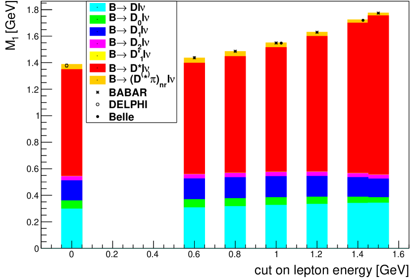
Figure 2: First electron moment $M_{1}$: Result of Fit 2 in Table 3 and the corresponding experimental data used.

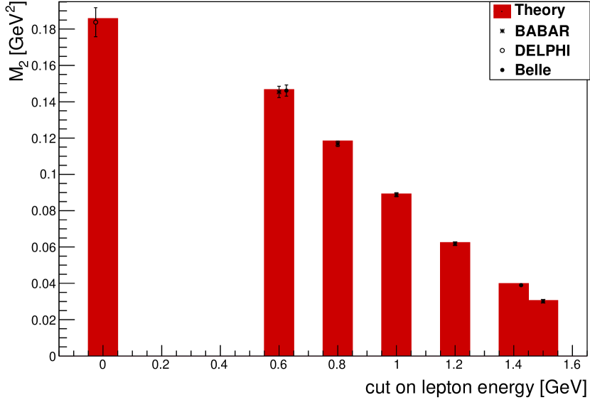
Figure 3: Second electron moment $M_{2}$: Result of Fit 2 in Table 3 and the corresponding experimental data used.

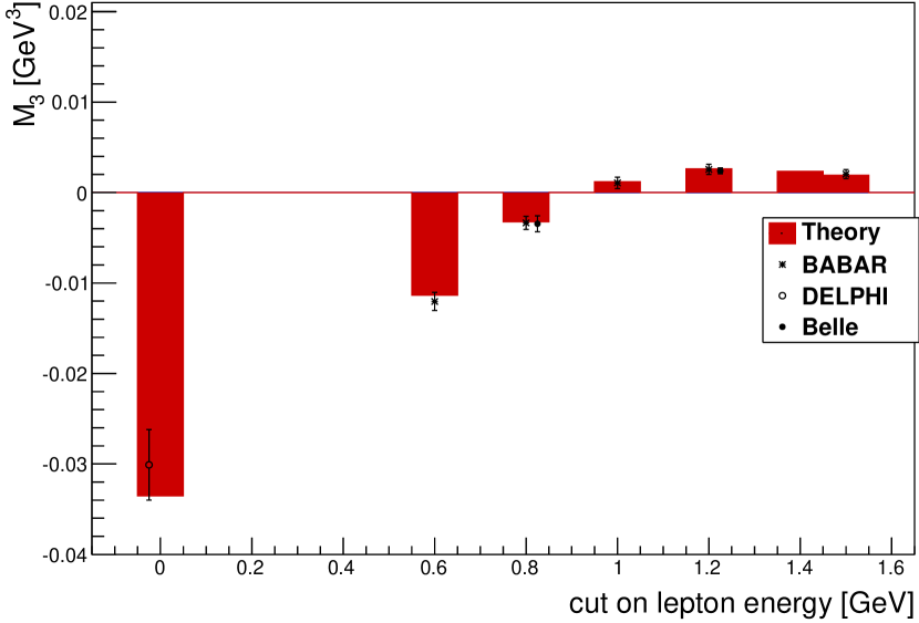
Figure 4: Third electron moment $M_{3}$: Result of Fit 2 in Table 3 and the corresponding experimental data used.

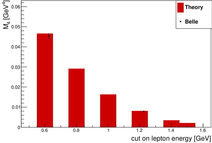
Figure 5: Fourth electron moment $M_{4}$: Result of Fit 2 in Table 3 and the corresponding experimental data used.

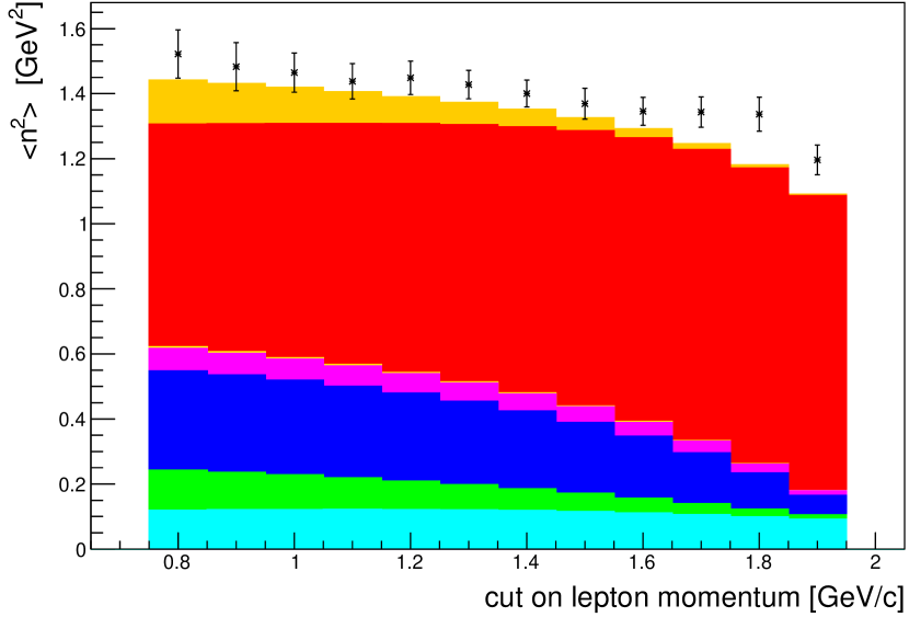
Figure 6: Energy-mass moment $\left\langle n^{2}\right\rangle$: Result of Fit 2 in Table 3 and the corresponding experimental data used. See legend of Fig. 2.

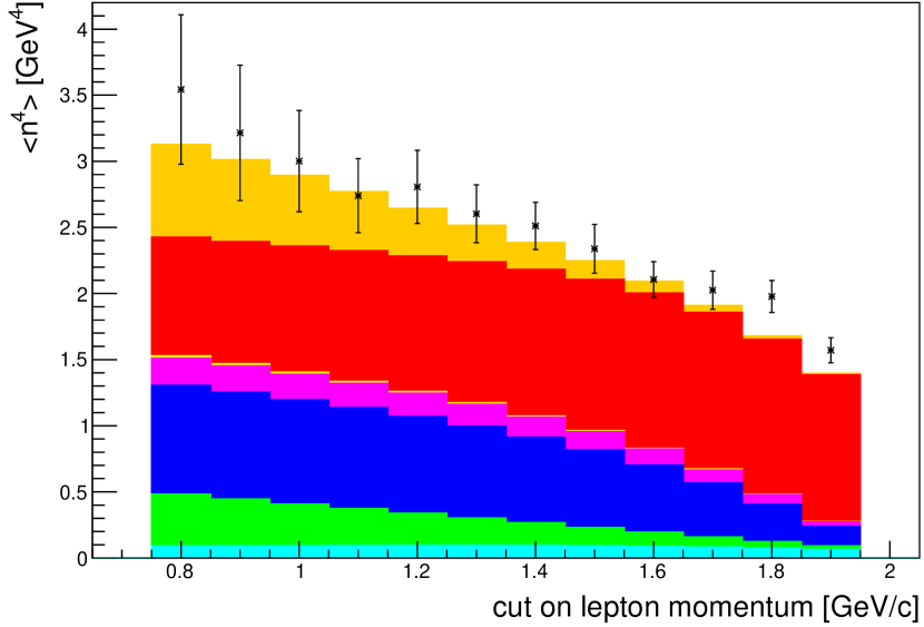
Figure 7: Energy-mass moment $\left\langle n^{4}\right\rangle$: Result of Fit 2 in Table 3 and the corresponding experimental data used. See legend of Fig. 2.

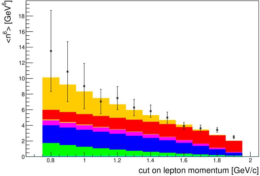
Figure 8: Energy-mass moment $\left\langle n^{6}\right\rangle$: Result of Fit 2 in Table 3 and the corresponding experimental data used. See legend of Fig. 2.

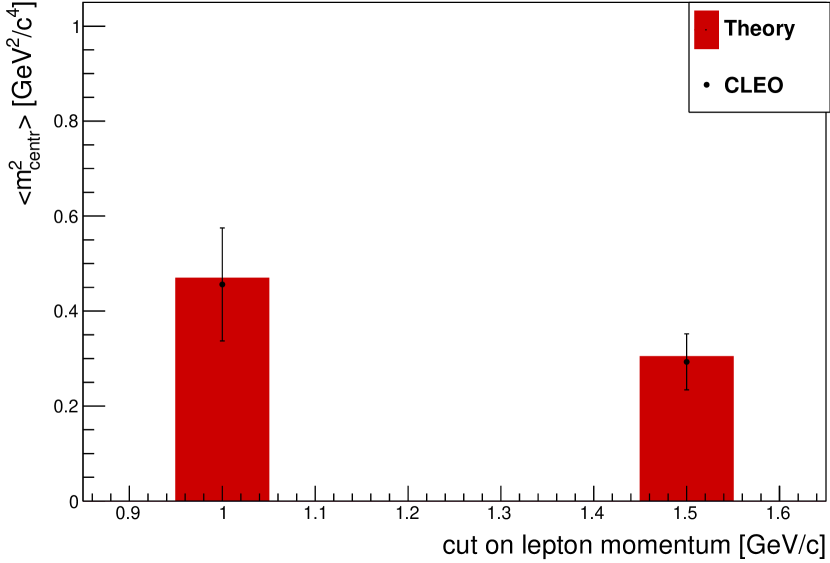
Figure 9: Central moment $\left\langle m^{2}_{centr}\right\rangle$: Result of Fit 2 in Table 3 and the corresponding experimental data used.

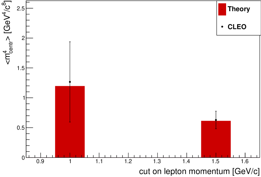
Figure 10: Central moment $\left\langle m^{4}_{centr}\right\rangle$: Result of Fit 2 in Table 3 and the corresponding experimental data used.

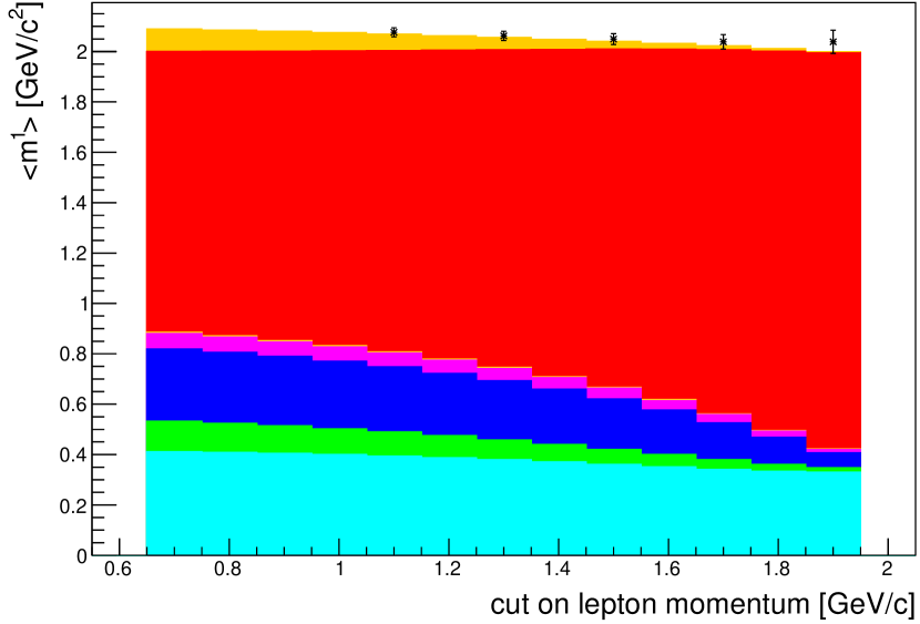
Figure 11: First hadronic mass moment $\left<m^{1}\right>$: Result of Fit 2 in Table 3 and the corresponding experimental data used. See legend of Fig. 2.

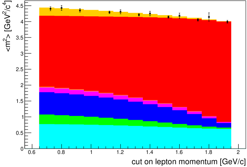
Figure 12: Second hadronic mass moment $\left<m^{2}\right>$: Result of Fit 2 in Table 3 and the corresponding experimental data used. See legend of Fig. 2.

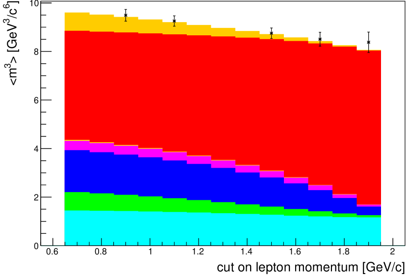
Figure 13: Third hadronic mass moment $\left<m^{3}\right>$: Result of Fit 2 in Table 3 and the corresponding experimental data used. See legend of Fig. 2.

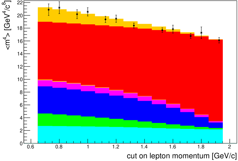
Figure 14: Fourth hadronic mass moment $\left<m^{4}\right>$: Result of Fit 2 in Table 3 and the corresponding experimental data used. See legend of Fig. 2.

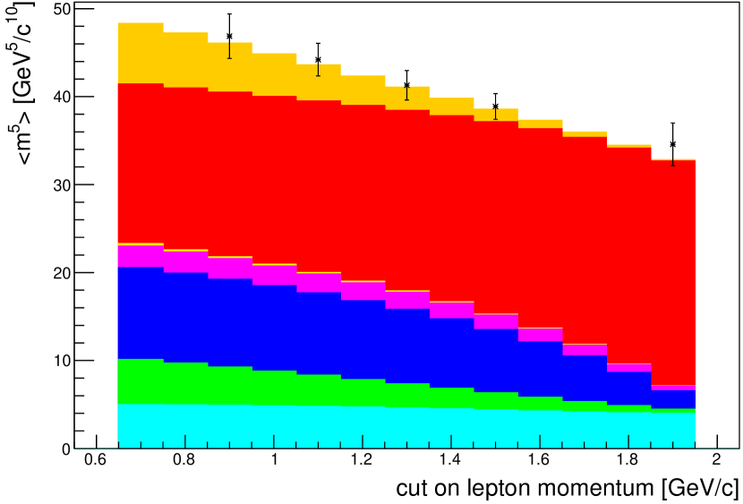
Figure 15: Fifth hadronic mass moment $\left<m^{5}\right>$: Result of Fit 2 in Table 3 and the corresponding experimental data used. See legend of Fig. 2.

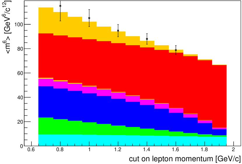
Figure 16: Sixth hadronic mass moment $\left<m^{6}\right>$: Result of Fit 2 in Table 3 and the corresponding experimental data used. See legend of Fig. 2.

Appendix E STUDIES OF PSEUDO-DATA

This appendix provides an example of the results obtained from the tests with a statistical ensemble of 1000 pseudo-data given in Fig.17-24.
For the fits on pseudo-datasets the distributions of the following two quantities are of particular interest:

• The normalized residuals $p$:
  The normalized residual $p_{i,n}$ associated with fit scenario $n$ and branching fraction $i$ is defined as

  $$p_{i,n}=\frac{\mathcal{B}_{i}^{0}(B\to X_{c}^{i}l\nu)-\mathcal{B}_{i}^{n}(B\to X_{c}^{i}l\nu)}{\sigma^{n}_{i}},$$ (E.1)

  where $\mathcal{B}_{i}^{0}(B\to X_{c}^{i}l\nu)$ is the value of the branching fraction of $B\to X_{c}^{i}l\nu$ decays used for the mixture of the nominal inclusive moments, $\mathcal{B}_{i}^{n}(B\to X_{c}^{i}l\nu)$ is the fitted result of the branching fraction of $B\to X_{c}^{i}l\nu$ decays of fit scenario $n$ and $\sigma^{n}_{i}$ is the corresponding calculated fit uncertainty. If the fit works properly, the expectation value of this quantity and its RMS (Root Mean Square) are

  $$\left\langle p\right\rangle=0,\qquad\sigma_{p}=1.$$ (E.2)

• The p-value $P$:
  If the fit results follow a Gaussian distribution with a standard deviation which is well estimated by the fit uncertainty, and if the fit model correctly describes the data the p-value defined as $P=\int\limits_{\chi^{2}_{0}}^{\infty}f({\chi^{2}})d\chi^{2}$, where $f({\chi^{2}})$ denotes the $\chi^{2}$ probability density function and $\chi_{0}^{2}$ the result of a particular fit, then $P$ follows a uniformly distributed random variable in the interval $\left[0,1\right]$.

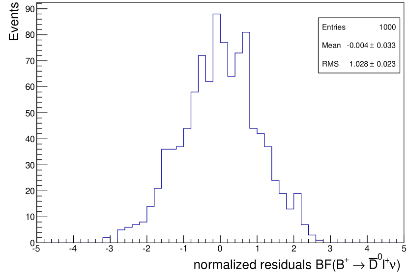
Figure 17: Distribution of normalized residuals for the results of $\mathcal{B}(B^{+}\to\overline{D}^{0}l^{+}\nu)$ corresponding to the fit scenario of Fit 2 in Table 3.

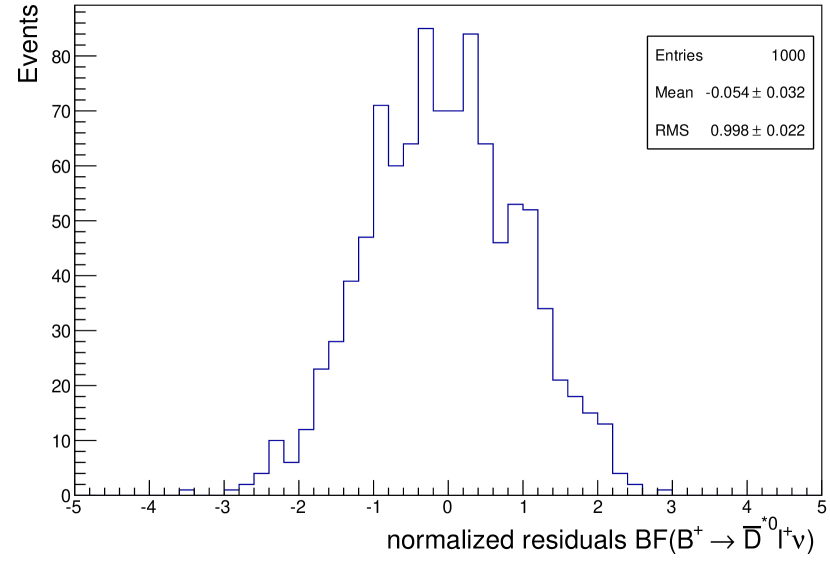
Figure 18: Distribution of normalized residuals for the results of $\mathcal{B}(B^{+}\to\overline{D}^{*0}l^{+}\nu)$ corresponding to the fit scenario of Fit 2 in Table 3.

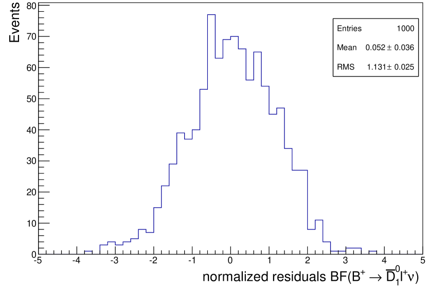
Figure 19: Distribution of normalized residuals for the results of $\mathcal{B}(B^{+}\to\overline{D}^{0}_{1}l^{+}\nu)$ corresponding to the fit scenario of Fit 2 in Table 3.

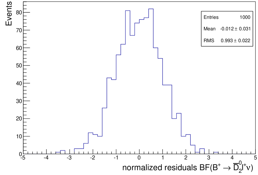
Figure 20: Distribution of normalized residuals for the results of $\mathcal{B}(B^{+}\to\overline{D}^{0}_{2}l^{+}\nu)$ corresponding to the fit scenario of Fit 2 in Table 3.

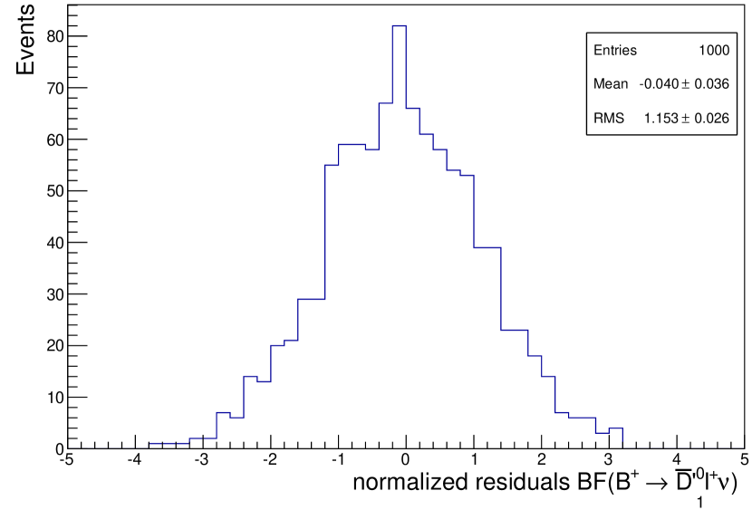
Figure 21: Distribution of normalized residuals for the results of $\mathcal{B}(B^{+}\to\overline{D}^{0}_{0}l^{+}\nu)$ corresponding to the fit scenario of Fit 2 in Table 3.

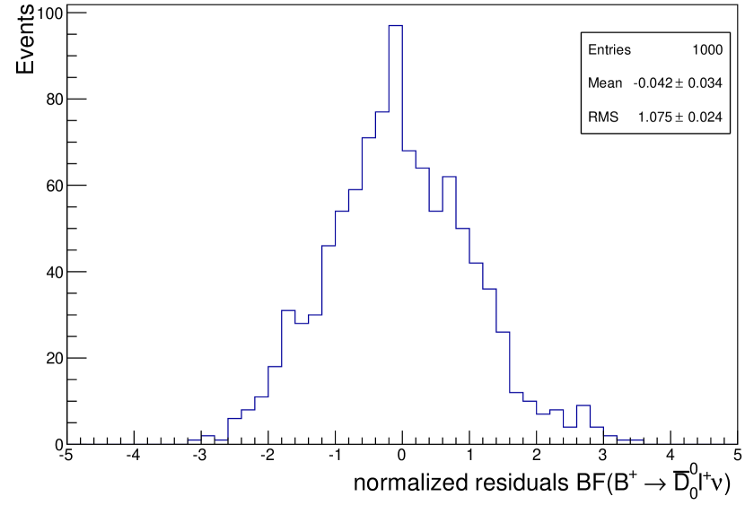
Figure 22: Distribution of normalized residuals for the results of $\mathcal{B}(B^{+}\to\overline{D}^{\prime 0}_{1}l^{+}\nu)$ corresponding to the fit scenario of Fit 2 in Table 3.

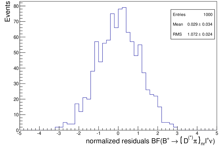
Figure 23: Distribution of normalized residuals for the results of $\mathcal{B}(B^{+}\to(D^{(*)}\pi)_{nr}l^{+}\nu)$ corresponding to the fit scenario of Fit 2 in Table 3.

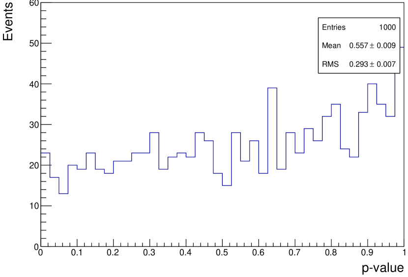
Figure 24: p-value distribution of the fits to pseudo data corresponding to the fit scenario of Fit 2 in Table 3.

Appendix F ADDITIONAL RESULTS

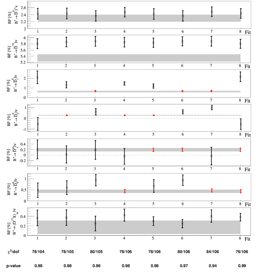
Figure 25: Depiction of the fit results as quoted in Tables 6 and 7 of Appendix F. In each subplot the abscissa indicates a distinctive fit scenario labeled by a number, whereas the ordinate represents the branching fraction. The results for a constrained branching fraction are depicted as red points, whereas the results for a unconstrained branching fraction are depicted as a black star. The grey bands correspond to the one-sigma error band of the corresponding direct branching-fraction measurements. If the ordinate includes zero, a dashed black line visualizes the zero line.

In this appendix, we quote in detail the results for all additional fit scenarios that were studied. The results are grouped in eight tables (6-13), corresponding to the related plots in Fig. 25-28.

$X_{c}$	Fit 1		Fit 2		Fit 3		Fit 4		Measured
	U/C	$\mathcal{B}[\%]$	U/C	$\mathcal{B}[\%]$	U/C	$\mathcal{B}[\%]$	U/C	$\mathcal{B}[\%]$	$\mathcal{B}[\%]$
$\overline{D}^{0}$	x/-	$2.43\pm 0.15$	x/-	$2.43\pm 0.15$	x/-	$2.37\pm 0.15$	x/-	$2.47\pm 0.14$	$2.30\pm 0.10$
$\overline{D}^{*0}$	x/-	$5.81\pm 0.16$	x/-	$5.86\pm 0.16$	x/-	$5.89\pm 0.16$	x/-	$5.86\pm 0.16$	$5.34\pm 0.12$
$\overline{D}_{1}^{0}$	x/-	$2.13\pm 0.67$	x/-	$1.33\pm 0.33$	x/x	$0.67\pm 0.07$	x/-	$1.47\pm 0.18$	$0.65\pm 0.07$
$\overline{D}_{2}^{0}$	x/-	$-0.52\pm 0.59$	x/x	$0.28\pm 0.03$	x/-	$0.61\pm 0.29$	x/x	$0.28\pm 0.03$	$0.28\pm 0.03$
$\overline{D}^{\prime 0}_{1}$	x/-	$0.21\pm 0.34$	x/-	$0.02\pm 0.31$	x/-	$0.19\pm 0.34$	x/-	$-0.04\pm 0.28$	$0.20\pm 0.06$
$\overline{D}_{0}^{0}$	x/-	$0.48\pm 0.33$	x/-	$0.60\pm 0.32$	x/-	$0.93\pm 0.26$	x/x	$0.44\pm 0.07$	$0.43\pm 0.07$
$\overline{D}^{\prime 0}$	-/-	-	-/-	-	-/-	-	-/-	-	-
$\overline{D}^{\prime*0}$	-/-	-	-/-	-	-/-	-	-/-	-	-
$(D^{(*)}\pi)_{nr}$	x/-	$0.36\pm 0.16$	x/-	$0.37\pm 0.16$	x/-	$0.25\pm 0.15$	x/-	$0.42\pm 0.13$	-
$\overline{D}^{0}_{1}/\overline{D}^{0}_{2}$	$1.61\pm 0.33$		$1.61\pm 0.33$		$1.27\pm 0.29$		$1.75\pm 0.18$		$0.94\pm 0.08$
$\overline{D}^{0}_{0}/\overline{D}^{\prime 0}_{1}$	$0.69\pm 0.54$		$0.62\pm 0.53$		$1.12\pm 0.50$		$0.40\pm 0.30$		$0.63\pm 0.10$
$\overline{D}^{0}_{0}/\overline{D}^{\prime 0}_{1}/(D^{(*)}\pi)_{nr}$	$1.06\pm 0.40$		$0.99\pm 0.39$		$1.37\pm 0.37$		$0.82\pm 0.21$		$0.63\pm 0.10$
$\sum_{i}X_{c}^{i}$	$10.90\pm 0.14$		$10.90\pm 0.14$		$10.90\pm 0.14$		$10.90\pm 0.14$		$9.21\pm 0.20$
$X_{c}$									$10.90\pm 0.14$
$\chi^{2}/dof$	75/104 = 0.73		77/105 = 0.74		80/105 = 0.77		77/106 = 0.73		-
p-value	0.98		0.98		0.96		0.98		-

Table 6: Results for moment fits of semileptonic decays $B^{+}\to X_{c}^{i}l^{+}\nu$ with hadronic final states $X_{c}^{i}$ containing $D$, $D^{*}$, any $D^{**}$, and $(D^{(*)}\pi)_{nr}$. Hereby, “U/C” stands for “used/constrained” and the “x” denotes “yes”, whereas “-” denotes “no”, respectively. The table is further described in the text of Section 5.

$X_{c}$	Fit 5		Fit 6		Fit 7		Fit 8		Measured
	U/C	$\mathcal{B}[\%]$	U/C	$\mathcal{B}[\%]$	U/C	$\mathcal{B}[\%]$	U/C	$\mathcal{B}[\%]$	$\mathcal{B}[\%]$
$\overline{D}^{0}$	x/-	$2.42\pm 0.15$	x/-	$2.37\pm 0.15$	x/-	$2.49\pm 0.14$	x/-	$2.44\pm 0.14$	$2.30\pm 0.10$
$\overline{D}^{*0}$	x/-	$5.84\pm 0.15$	x/-	$5.88\pm 0.15$	x/-	$5.89\pm 0.16$	x/-	$5.80\pm 0.15$	$5.34\pm 0.12$
$\overline{D}_{1}^{0}$	x/-	$1.20\pm 0.23$	x/x	$0.67\pm 0.07$	x/x	$0.68\pm 0.07$	x/-	$2.19\pm 0.52$	$0.65\pm 0.07$
$\overline{D}_{2}^{0}$	x/x	$0.28\pm 0.03$	x/-	$0.60\pm 0.19$	x/-	$0.99\pm 0.20$	x/-	$-0.54\pm 0.50$	$0.28\pm 0.03$
$\overline{D}^{\prime 0}_{1}$	x/x	$0.19\pm 0.06$	x/x	$0.19\pm 0.06$	x/-	$-0.03\pm 0.32$	x/x	$0.19\pm 0.06$	$0.20\pm 0.06$
$\overline{D}_{0}^{0}$	x/-	$0.67\pm 0.29$	x/-	$0.94\pm 0.24$	x/x	$0.47\pm 0.07$	x/x	$0.44\pm 0.07$	$0.43\pm 0.07$
$\overline{D}^{\prime 0}$	-/-	-	-/-	-	-/-	-	-/-	-	-
$\overline{D}^{\prime*0}$	-/-	-	-/-	-	-/-	-	-/-	-	-
$(D^{(*)}\pi)_{nr}$	x/-	$0.30\pm 0.09$	x/-	$0.25\pm 0.09$	x/-	$0.40\pm 0.13$	x/-	$0.38\pm 0.08$	-
$\overline{D}^{0}_{1}/\overline{D}^{0}_{2}$	$1.48\pm 0.22$		$1.27\pm 0.18$		$1.67\pm 0.19$		$1.65\pm 0.11$		$0.94\pm 0.08$
$\overline{D}^{0}_{0}/\overline{D}^{\prime 0}_{1}$	$0.86\pm 0.30$		$1.13\pm 0.25$		$0.44\pm 0.33$		$0.63\pm 0.09$		$0.63\pm 0.10$
$\overline{D}^{0}_{0}/\overline{D}^{\prime 0}_{1}/(D^{(*)}\pi)_{nr}$	$1.16\pm 0.25$		$1.38\pm 0.22$		$0.84\pm 0.24$		$1.01\pm 0.10$		$0.63\pm 0.10$
$\sum_{i}X_{c}^{i}$	$10.90\pm 0.14$		$10.90\pm 0.14$		$10.89\pm 0.14$		$10.90\pm 0.14$		$9.21\pm 0.20$
$X_{c}$									$10.90\pm 0.14$
$\chi^{2}/dof$	77/106 = 0.74		80/106 = 0.76		83/106 = 0.79		76/106 = 0.72		-
p-value	0.98		0.97		0.94		0.99		-

Table 7: Results for moment fits of semileptonic decays $B^{+}\to X_{c}^{i}l^{+}\nu$ with hadronic final states $X_{c}^{i}$ containing $D$, $D^{*}$, any $D^{**}$, and $(D^{(*)}\pi)_{nr}$. Hereby, “U/C” stands for “used/constrained” and the “x” denotes “yes”, whereas “-” denotes “no”, respectively. The table is further described in the text of Section 5.

$X_{c}$	Fit 9		Fit 10		Fit 11		Fit 12		Measured
	U/C	$\mathcal{B}[\%]$	U/C	$\mathcal{B}[\%]$	U/C	$\mathcal{B}[\%]$	U/C	$\mathcal{B}[\%]$	$\mathcal{B}[\%]$
$\overline{D}^{0}$	x/x	$2.40\pm 0.08$	x/x	$2.41\pm 0.08$	x/x	$2.44\pm 0.08$	x/x	$2.42\pm 0.08$	$2.30\pm 0.10$
$\overline{D}^{*0}$	x/x	$5.55\pm 0.09$	x/x	$5.59\pm 0.09$	x/x	$5.60\pm 0.09$	x/x	$5.60\pm 0.09$	$5.34\pm 0.12$
$\overline{D}_{1}^{0}$	x/-	$2.26\pm 0.64$	x/-	$1.10\pm 0.30$	x/-	$1.38\pm 0.18$	x/-	$1.19\pm 0.20$	$0.65\pm 0.07$
$\overline{D}_{2}^{0}$	x/-	$-0.87\pm 0.56$	x/x	$0.28\pm 0.03$	x/x	$0.28\pm 0.03$	x/x	$0.28\pm 0.03$	$0.28\pm 0.03$
$\overline{D}^{\prime 0}_{1}$	x/-	$0.55\pm 0.32$	x/-	$0.32\pm 0.29$	x/-	$0.19\pm 0.27$	x/x	$0.20\pm 0.06$	$0.20\pm 0.06$
$\overline{D}_{0}^{0}$	x/-	$0.60\pm 0.30$	x/-	$0.78\pm 0.29$	x/x	$0.46\pm 0.07$	x/-	$0.73\pm 0.26$	$0.43\pm 0.07$
$\overline{D}^{\prime 0}$	-/-	-	-/-	-	-/-	-	-/-	-	-
$\overline{D}^{\prime*0}$	-/-	-	-/-	-	-/-	-	-/-	-	-
$(D^{(*)}\pi)_{nr}$	x/-	$0.21\pm 0.15$	x/-	$0.20\pm 0.15$	x/-	$0.31\pm 0.11$	x/-	$0.25\pm 0.09$	-
$\overline{D}^{0}_{1}/\overline{D}^{0}_{2}$	$1.40\pm 0.30$		$1.38\pm 0.30$		$1.66\pm 0.17$		$1.47\pm 0.20$		$0.94\pm 0.08$
$\overline{D}^{0}_{0}/\overline{D}^{\prime 0}_{1}$	$1.15\pm 0.49$		$1.10\pm 0.49$		$0.64\pm 0.29$		$0.93\pm 0.27$		$0.63\pm 0.10$
$\overline{D}^{0}_{0}/\overline{D}^{\prime 0}_{1}/(D^{(*)}\pi)_{nr}$	$1.36\pm 0.36$		$1.30\pm 0.36$		$0.96\pm 0.20$		$1.18\pm 0.22$		$0.63\pm 0.10$
$\sum_{i}X_{c}^{i}$	$10.71\pm 0.12$		$10.68\pm 0.12$		$10.65\pm 0.12$		$10.67\pm 0.12$		$9.21\pm 0.20$
$X_{c}$									$10.90\pm 0.14$
$\chi^{2}/dof$	83/106 = 0.79		88/107 = 0.82		89/108 = 0.83		88/108 = 0.82		-
p-value	0.94		0.91		0.90		0.92		-

Table 8: Results for moment fits of semileptonic decays $B^{+}\to X_{c}^{i}l^{+}\nu$ with hadronic final states $X_{c}^{i}$ containing $D$, $D^{*}$, any $D^{**}$, and $(D^{(*)}\pi)_{nr}$. Hereby, “U/C” stands for “used/constrained” and the “x” denotes “yes”, whereas “-” denotes “no”, respectively. The table is further described in the text of Section 5.

$X_{c}$	Fit 13		Fit 14		Fit 15		Fit 16		Measured
	U/C	$\mathcal{B}[\%]$	U/C	$\mathcal{B}[\%]$	U/C	$\mathcal{B}[\%]$	U/C	$\mathcal{B}[\%]$	$\mathcal{B}[\%]$
$\overline{D}^{0}$	x/x	$2.40\pm 0.08$	x/x	$2.38\pm 0.08$	x/x	$2.44\pm 0.08$	x/x	$2.42\pm 0.08$	$2.30\pm 0.10$
$\overline{D}^{*0}$	x/x	$5.61\pm 0.09$	x/x	$5.58\pm 0.09$	x/x	$5.61\pm 0.09$	x/x	$5.58\pm 0.09$	$5.34\pm 0.12$
$\overline{D}_{1}^{0}$	x/x	$0.67\pm 0.07$	x/x	$0.67\pm 0.07$	x/x	$0.69\pm 0.07$	x/-	$2.38\pm 0.50$	$0.65\pm 0.07$
$\overline{D}_{2}^{0}$	x/-	$0.60\pm 0.17$	x/-	$0.37\pm 0.27$	x/-	$0.83\pm 0.20$	x/-	$-0.71\pm 0.48$	$0.28\pm 0.03$
$\overline{D}^{\prime 0}_{1}$	x/x	$0.21\pm 0.06$	x/-	$0.55\pm 0.32$	x/-	$0.30\pm 0.30$	x/x	$0.21\pm 0.06$	$0.20\pm 0.06$
$\overline{D}_{0}^{0}$	x/-	$0.98\pm 0.22$	x/-	$1.07\pm 0.23$	x/x	$0.49\pm 0.07$	x/x	$0.44\pm 0.07$	$0.43\pm 0.07$
$\overline{D}^{\prime 0}$	-/-	-	-/-	-	-/-	-	-/-	-	-
$\overline{D}^{\prime*0}$	-/-	-	-/-	-	-/-	-	-/-	-	-
$(D^{(*)}\pi)_{nr}$	x/-	$0.19\pm 0.08$	x/-	$0.07\pm 0.14$	x/-	$0.27\pm 0.12$	x/-	$0.36\pm 0.07$	-
$\overline{D}^{0}_{1}/\overline{D}^{0}_{2}$	$1.27\pm 0.16$		$1.04\pm 0.26$		$1.52\pm 0.18$		$1.67\pm 0.11$		$0.94\pm 0.08$
$\overline{D}^{0}_{0}/\overline{D}^{\prime 0}_{1}$	$1.19\pm 0.23$		$1.62\pm 0.45$		$0.79\pm 0.31$		$0.65\pm 0.09$		$0.63\pm 0.10$
$\overline{D}^{0}_{0}/\overline{D}^{\prime 0}_{1}/(D^{(*)}\pi)_{nr}$	$1.38\pm 0.19$		$1.69\pm 0.34$		$1.06\pm 0.23$		$1.00\pm 0.10$		$0.63\pm 0.10$
$\sum_{i}X_{c}^{i}$	$10.66\pm 0.12$		$10.69\pm 0.12$		$10.63\pm 0.12$		$10.67\pm 0.12$		$9.21\pm 0.20$
$X_{c}$									$10.90\pm 0.14$
$\chi^{2}/dof$	91/108 = 0.84		90/107 = 0.84		96/108 = 0.90		85/108 = 0.79		-
p-value	0.88		0.88		0.77		0.95		-

Table 9: Results for moment fits of semileptonic decays $B^{+}\to X_{c}^{i}l^{+}\nu$ with hadronic final states $X_{c}^{i}$ containing $D$, $D^{*}$, any $D^{**}$, and $(D^{(*)}\pi)_{nr}$. Hereby, “U/C” stands for “used/constrained” and the “x” denotes “yes”, whereas “-” denotes “no”, respectively. The table is further described in the text of Section 5.

$X_{c}$	Fit 17		Fit 18		Fit 19		Fit 20		Measured
	U/C	$\mathcal{B}[\%]$	U/C	$\mathcal{B}[\%]$	U/C	$\mathcal{B}[\%]$	U/C	$\mathcal{B}[\%]$	$\mathcal{B}[\%]$
$\overline{D}^{0}$	x/x	$2.34\pm 0.08$	x/x	$2.35\pm 0.08$	x/x	$2.34\pm 0.08$	x/-	$2.61\pm 0.14$	$2.30\pm 0.10$
$\overline{D}^{*0}$	x/-	$5.92\pm 0.14$	x/-	$5.86\pm 0.15$	x/-	$5.87\pm 0.13$	x/x	$5.53\pm 0.09$	$5.34\pm 0.12$
$\overline{D}_{1}^{0}$	x/-	$1.24\pm 0.30$	x/-	$2.23\pm 0.53$	x/-	$2.05\pm 0.66$	x/-	$1.34\pm 0.33$	$0.65\pm 0.07$
$\overline{D}_{2}^{0}$	x/x	$0.28\pm 0.03$	x/-	$-0.60\pm 0.56$	x/-	$-0.50\pm 0.54$	x/x	$0.28\pm 0.03$	$0.28\pm 0.03$
$\overline{D}^{\prime 0}_{1}$	x/-	$0.05\pm 0.31$	x/-	$0.20\pm 0.33$	x/x	$0.20\pm 0.06$	x/-	$0.19\pm 0.30$	$0.20\pm 0.06$
$\overline{D}_{0}^{0}$	x/-	$0.69\pm 0.29$	x/x	$0.44\pm 0.07$	x/-	$0.56\pm 0.29$	x/-	$0.55\pm 0.31$	$0.43\pm 0.07$
$\overline{D}^{\prime 0}$	-/-	-	-/-	-	-/-	-	-/-	-	-
$\overline{D}^{\prime*0}$	-/-	-	-/-	-	-/-	-	-/-	-	-
$(D^{(*)}\pi)_{nr}$	x/-	$0.36\pm 0.16$	x/-	$0.40\pm 0.13$	x/-	$0.37\pm 0.10$	x/-	$0.27\pm 0.16$	-
$\overline{D}^{0}_{1}/\overline{D}^{0}_{2}$	$1.52\pm 0.30$		$1.63\pm 0.19$		$1.55\pm 0.22$		$1.62\pm 0.32$		$0.94\pm 0.08$
$\overline{D}^{0}_{0}/\overline{D}^{\prime 0}_{1}$	$0.75\pm 0.50$		$0.65\pm 0.34$		$0.76\pm 0.30$		$0.73\pm 0.52$		$0.63\pm 0.10$
$\overline{D}^{0}_{0}/\overline{D}^{\prime 0}_{1}/(D^{(*)}\pi)_{nr}$	$1.10\pm 0.36$		$1.04\pm 0.24$		$1.13\pm 0.24$		$1.00\pm 0.39$		$0.63\pm 0.10$
$\sum_{i}X_{c}^{i}$	$10.88\pm 0.14$		$10.88\pm 0.14$		$10.88\pm 0.14$		$10.77\pm 0.13$		$9.21\pm 0.20$
$X_{c}$									$10.90\pm 0.14$
$\chi^{2}/dof$	78/106 = 0.74		76/106 = 0.72		76/106 = 0.72		84/106 = 0.80		-
p-value	0.98		0.99		0.99		0.94		-

Table 10: Results for moment fits of semileptonic decays $B^{+}\to X_{c}^{i}l^{+}\nu$ with hadronic final states $X_{c}^{i}$ containing $D$, $D^{*}$, any $D^{**}$, and $(D^{(*)}\pi)_{nr}$. Hereby, “U/C” stands for “used/constrained” and the “x” denotes “yes”, whereas “-” denotes “no”, respectively. The table is further described in the text of Section 5.

$X_{c}$	Fit 21		Fit 22		Fit 23		Fit 24		Measured
	U/C	$\mathcal{B}[\%]$	U/C	$\mathcal{B}[\%]$	U/C	$\mathcal{B}[\%]$	U/C	$\mathcal{B}[\%]$	$\mathcal{B}[\%]$
$\overline{D}^{0}$	x/-	$2.57\pm 0.12$	x/-	$2.61\pm 0.13$	x/-	$2.53\pm 0.14$	x/x	$2.32\pm 0.08$	$2.30\pm 0.10$
$\overline{D}^{*0}$	x/x	$5.51\pm 0.10$	x/x	$5.52\pm 0.09$	x/x	$5.54\pm 0.09$	x/-	$5.91\pm 0.14$	$5.34\pm 0.12$
$\overline{D}_{1}^{0}$	x/-	$2.35\pm 0.52$	x/-	$2.41\pm 0.66$	x/x	$0.67\pm 0.07$	x/x	$0.67\pm 0.07$	$0.65\pm 0.07$
$\overline{D}_{2}^{0}$	x/-	$-0.76\pm 0.55$	x/-	$-0.65\pm 0.53$	x/-	$0.53\pm 0.29$	x/-	$0.57\pm 0.28$	$0.28\pm 0.03$
$\overline{D}^{\prime 0}_{1}$	x/-	$0.42\pm 0.31$	x/x	$0.20\pm 0.06$	x/-	$0.44\pm 0.33$	x/-	$0.20\pm 0.34$	$0.20\pm 0.06$
$\overline{D}_{0}^{0}$	x/x	$0.43\pm 0.07$	x/-	$0.33\pm 0.31$	x/-	$0.93\pm 0.25$	x/-	$0.96\pm 0.24$	$0.43\pm 0.07$
$\overline{D}^{\prime 0}$	-/-	-	-/-	-	-/-	-	-/-	-	-
$\overline{D}^{\prime*0}$	-/-	-	-/-	-	-/-	-	-/-	-	-
$(D^{(*)}\pi)_{nr}$	x/-	$0.26\pm 0.12$	x/-	$0.35\pm 0.10$	x/-	$0.11\pm 0.14$	x/-	$0.25\pm 0.15$	-
$\overline{D}^{0}_{1}/\overline{D}^{0}_{2}$	$1.58\pm 0.19$		$1.76\pm 0.23$		$1.20\pm 0.29$		$1.24\pm 0.27$		$0.94\pm 0.08$
$\overline{D}^{0}_{0}/\overline{D}^{\prime 0}_{1}$	$0.85\pm 0.33$		$0.54\pm 0.31$		$1.37\pm 0.49$		$1.17\pm 0.48$		$0.63\pm 0.10$
$\overline{D}^{0}_{0}/\overline{D}^{\prime 0}_{1}/(D^{(*)}\pi)_{nr}$	$1.12\pm 0.24$		$0.89\pm 0.25$		$1.48\pm 0.37$		$1.41\pm 0.35$		$0.63\pm 0.10$
$\sum_{i}X_{c}^{i}$	$10.78\pm 0.13$		$10.77\pm 0.13$		$10.75\pm 0.13$		$10.89\pm 0.14$		$9.21\pm 0.20$
$X_{c}$									$10.90\pm 0.14$
$\chi^{2}/dof$	81/106 = 0.77		81/106 = 0.77		88/106 = 0.83		80/106 = 0.76		-
p-value	0.96		0.96		0.90		0.97		-

Table 11: Results for moment fits of semileptonic decays $B^{+}\to X_{c}^{i}l^{+}\nu$ with hadronic final states $X_{c}^{i}$ containing $D$, $D^{*}$, any $D^{**}$, and $(D^{(*)}\pi)_{nr}$. Hereby, “U/C” stands for “used/constrained” and the “x” denotes “yes”, whereas “-” denotes “no”, respectively. The table is further described in the text of Section 5.

$X_{c}$	Fit 25		Fit 26		Fit 27		Fit 28		Measured
	U/C	$\mathcal{B}[\%]$	U/C	$\mathcal{B}[\%]$	U/C	$\mathcal{B}[\%]$	U/C	$\mathcal{B}[\%]$	$\mathcal{B}[\%]$
$\overline{D}^{0}$	x/x	$2.42\pm 0.08$	x/x	$2.42\pm 0.08$	x/x	$2.41\pm 0.08$	x/x	$2.42\pm 0.08$	$2.30\pm 0.10$
$\overline{D}^{*0}$	x/x	$5.63\pm 0.09$	x/x	$5.65\pm 0.09$	x/x	$5.62\pm 0.09$	x/x	$5.56\pm 0.09$	$5.34\pm 0.12$
$\overline{D}_{1}^{0}$	x/x	$0.78\pm 0.07$	x/x	$0.79\pm 0.07$	x/x	$0.79\pm 0.07$	x/-	$1.72\pm 0.23$	$0.65\pm 0.07$
$\overline{D}_{2}^{0}$	x/x	$0.30\pm 0.03$	x/x	$0.30\pm 0.03$	x/x	$0.30\pm 0.03$	x/x	$0.28\pm 0.03$	$0.28\pm 0.03$
$\overline{D}^{\prime 0}_{1}$	x/x	$0.22\pm 0.06$	x/x	$0.23\pm 0.06$	x/x	$0.22\pm 0.06$	x/-	$-0.13\pm 0.51$	$0.20\pm 0.06$
$\overline{D}_{0}^{0}$	x/x	$0.56\pm 0.07$	x/x	$0.56\pm 0.07$	x/x	$0.56\pm 0.07$	x/x	$0.44\pm 0.07$	$0.43\pm 0.07$
$\overline{D}^{\prime 0}$	x/-	$0.35\pm 0.12$	-/-	-	x/-	$0.50\pm 0.37$	x/-	$0.79\pm 0.63$	-
$\overline{D}^{\prime*0}$	-/-	-	x/-	$0.27\pm 0.10$	x/-	$-0.14\pm 0.32$	x/-	$-0.85\pm 0.46$	-
$(D^{(*)}\pi)_{nr}$	x/-	$0.31\pm 0.07$	x/-	$0.31\pm 0.07$	x/-	$0.31\pm 0.07$	x/-	$0.46\pm 0.17$	-
$\overline{D}^{0}_{1}+\overline{D}^{0}_{2}$	$1.08\pm 0.07$		$1.09\pm 0.07$		$1.09\pm 0.07$		$2.00\pm 0.23$		$0.94\pm 0.08$
$\overline{D}^{0}_{0}+\overline{D}^{\prime 0}_{1}$	$0.78\pm 0.09$		$0.79\pm 0.09$		$0.78\pm 0.09$		$0.32\pm 0.52$		$0.63\pm 0.10$
$\overline{D}^{0}_{0}/\overline{D}^{\prime 0}_{1}+(D^{(*)}\pi)_{nr}$	$1.09\pm 0.10$		$1.11\pm 0.10$		$1.09\pm 0.10$		$0.78\pm 0.38$		$0.63\pm 0.10$
$\sum_{i}X_{c}^{i}$	$10.56\pm 0.12$		$10.54\pm 0.12$		$10.57\pm 0.12$		$10.69\pm 0.12$		$9.21\pm 0.20$
$X_{c}$									$10.90\pm 0.14$
$\chi^{2}/dof$	110/109 = 1.01		111/109 = 1.03		110/108 = 1.02		84/106 = 0.79		-
p-value	0.45		0.41		0.43		0.94		-

Table 12: Results for moment fits of semileptonic decays $B^{+}\to X_{c}^{i}l^{+}\nu$ with hadronic final states $X_{c}^{i}$ containing $D$, $D^{*}$, any $D^{**}$, $D^{\prime(*)}$, and $(D^{(*)}\pi)_{nr}$. Hereby, “U/C” stands for “used/constrained” and the “x” denotes “yes”, whereas “-” denotes “no”, respectively. The table is further described in the text of Section 5.

$X_{c}$	Fit 29		Fit 30		Fit 31		Fit 32		Measured
	U/C	$\mathcal{B}[\%]$	U/C	$\mathcal{B}[\%]$	U/C	$\mathcal{B}[\%]$	U/C	$\mathcal{B}[\%]$	$\mathcal{B}[\%]$
$\overline{D}^{0}$	x/x	$2.44\pm 0.08$	x/-	$2.39\pm 0.13$	x/-	$2.30\pm 0.14$	x/-	$2.52\pm 0.14$	$2.30\pm 0.10$
$\overline{D}^{*0}$	x/x	$5.57\pm 0.09$	x/-	$5.92\pm 0.15$	x/-	$5.84\pm 0.17$	x/-	$5.79\pm 0.17$	$5.34\pm 0.12$
$\overline{D}_{1}^{0}$	x/-	$1.45\pm 0.18$	x/x	$0.77\pm 0.07$	x/x	$0.68\pm 0.07$	x/x	$0.66\pm 0.07$	$0.65\pm 0.07$
$\overline{D}_{2}^{0}$	x/x	$0.28\pm 0.03$	x/x	$0.30\pm 0.03$	x/x	$0.29\pm 0.03$	x/-	$1.25\pm 0.24$	$0.28\pm 0.03$
$\overline{D}^{\prime 0}_{1}$	x/-	$0.56\pm 0.37$	x/x	$0.21\pm 0.06$	x/-	$0.61\pm 0.38$	x/-	$0.40\pm 0.39$	$0.20\pm 0.06$
$\overline{D}_{0}^{0}$	x/x	$0.46\pm 0.07$	x/x	$0.55\pm 0.07$	x/-	$1.15\pm 0.18$	x/x	$0.46\pm 0.07$	$0.43\pm 0.07$
$\overline{D}^{\prime 0}$	x/-	$-0.33\pm 0.22$	x/-	$0.33\pm 0.12$	x/-	$-0.10\pm 0.23$	x/-	$-0.52\pm 0.27$	-
$\overline{D}^{\prime*0}$	-/-	-	-/-	-	-/-	-	-/-	-	-
$(D^{(*)}\pi)_{nr}$	x/-	$0.25\pm 0.12$	x/-	$0.36\pm 0.08$	x/-	$0.10\pm 0.13$	x/-	$0.32\pm 0.14$	-
$\overline{D}^{0}_{1}/\overline{D}^{0}_{2}$	$1.74\pm 0.18$		$1.07\pm 0.07$		$0.97\pm 0.08$		$1.92\pm 0.23$		$0.94\pm 0.08$
$\overline{D}^{0}_{0}/\overline{D}^{\prime 0}_{1}$	$1.01\pm 0.38$		$0.76\pm 0.09$		$1.77\pm 0.40$		$0.86\pm 0.40$		$0.63\pm 0.10$
$\overline{D}^{0}_{0}/\overline{D}^{\prime 0}_{1}/(D^{(*)}\pi)_{nr}$	$1.26\pm 0.29$		$1.11\pm 0.10$		$1.87\pm 0.30$		$1.18\pm 0.29$		$0.63\pm 0.10$
$\sum_{i}X_{c}^{i}$	$10.67\pm 0.12$		$10.84\pm 0.14$		$10.89\pm 0.14$		$10.89\pm 0.14$		$9.21\pm 0.20$
$X_{c}$									$10.90\pm 0.14$
$\chi^{2}/dof$	87/107 = 0.82		97/107 = 0.91		81/105 = 0.78		80/105 = 0.77		-
p-value	0.92		0.73		0.96		0.96		-

Table 13: Results for moment fits of semileptonic decays $B^{+}\to X_{c}^{i}l^{+}\nu$ with hadronic final states $X_{c}^{i}$ containing $D$, $D^{*}$, any $D^{**}$, $D^{\prime(*)}$, and $(D^{(*)}\pi)_{nr}$. Hereby, “U/C” stands for “used/constrained” and the “x” denotes “yes”, whereas “-” denotes “no”, respectively. The table is further described in the text of Section 5.

Appendix G PLOTS OF ADDITIONAL RESULTS

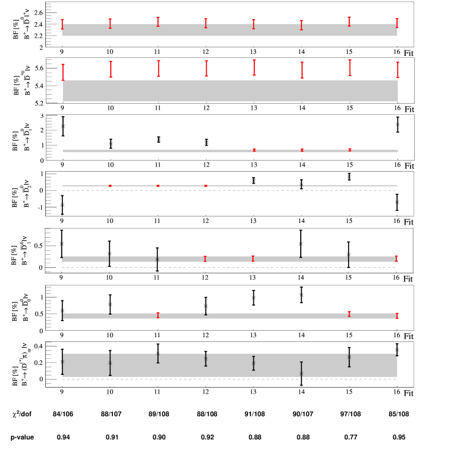
Figure 26: Depiction of the fit results as quoted in Tables 8 and 9 of Appendix F. In each subplot the abscissa indicates a distinctive fit scenario labeled by a number, whereas the ordinate represents the branching fraction. The results for a constrained branching fraction are depicted as red points, whereas the results for a unconstrained branching fraction are depicted as a black star. The grey bands correspond to the one-sigma error band of the corresponding direct branching-fraction measurements. If the ordinate includes zero, a dashed black line visualizes the zero line.

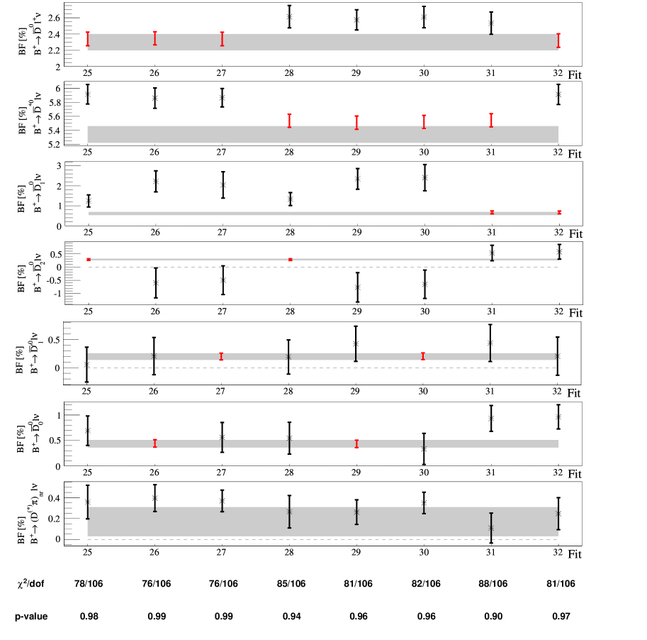
Figure 27: Depiction of the fit results as quoted in Tables 10 and 11 of Appendix F. In each subplot the abscissa indicates a distinctive fit scenario labeled by a number, whereas the ordinate represents the branching fraction. The results for a constrained branching fraction are depicted as red points, whereas the results for a unconstrained branching fraction are depicted as a black star. The grey bands correspond to the one-sigma error band of the corresponding direct branching-fraction measurements. If the ordinate includes zero, a dashed black line visualizes the zero line.

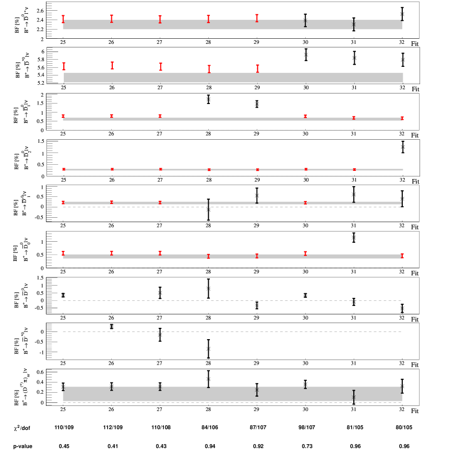
Figure 28: Depiction of the fit results as quoted in Tables 12 and 13 of Appendix F. In each subplot the abscissa indicates a distinctive fit scenario labeled by a number, whereas the ordinate represents the branching fraction. The results for a constrained branching fraction are depicted as red points, whereas the results for a unconstrained branching fraction are depicted as a black star. The grey bands correspond to the one-sigma error band of the corresponding direct branching-fraction measurements. If the ordinate includes zero, a dashed black line visualizes the zero line.

Appendix H RESULTS FOR SELECTED SETS OF INPUTS

In this appendix, we show the results for fits were different sets of experimental inputs are used. This is done to check if particlar measurements drive e.g. $\mathcal{B}(B^{+}\to\overline{D}^{*0}l^{+}\nu)$ to the large observed values and which fit inputs have the strongest impact on the final fit uncertainties. In these fits we always constrain $\mathcal{B}(B^{+}\to\overline{D}^{0}l^{+}\nu)$ and $\mathcal{B}(B^{+}\to\overline{D}_{0}^{0}l^{+}\nu)$ to their measured value and present two series of fits in which we either constrain $\mathcal{B}(B^{+}\to\overline{D}_{2}^{0}l^{+}\nu)$ or $\mathcal{B}(B^{+}\to\overline{D}_{1}^{0}l^{+}\nu)$.
Accordingly, in Fit 1, respectively, Fit 6 only lepton energy moments are used. In Fit 2 and Fit 7 we use only the combined hadronic mass-energy moments, which were only measured by the ${\displaystyle B}\!{\scriptstyle A}\!{\displaystyle B}\!{\scriptstyle{A\!R}}$  experiment, whereas in Fit 3 and Fit 8 we use only hadronic mass moments. In Fit 4 and Fit 9, we use combined hadronic mass-energy moments (measured only by the ${\displaystyle B}\!{\scriptstyle A}\!{\displaystyle B}\!{\scriptstyle{A\!R}}$  ), but omit the two data points for the lower lepton momentum cut-off equal to 1.8 GeV/c and 1.9 GeV/c. This check was performed since these two data points can not be described very well by the fitted moment distribution. Furthermore, in Fit 5 and Fit 10, we use only the hadronic mass moments but remove the Belle measurements from the list of inputs.
We find that $\mathcal{B}(B^{+}\to\overline{D}^{*0}l^{+}\nu)$ is mainly enlarged due to the hadronic mass-energy moments and in particular due to the mass moments. The fit uncertainties decrease in size when using either only combined hadronic energy-mass moments, or only electron energy moments, or only hadronic mass moments.

$X_{c}$	Fit 1		Fit 2		Fit 3		Fit 4		Fit 5		Measured
	U/C	$\mathcal{B}[\%]$	U/C	$\mathcal{B}[\%]$	U/C	$\mathcal{B}[\%]$	U/C	$\mathcal{B}[\%]$	U/C	$\mathcal{B}[\%]$	$[\%]$
$\overline{D}^{0}$	x/x	$2.30\pm 0.10$	x/x	$2.25\pm 0.10$	x/x	$2.31\pm 0.09$	x/x	$2.25\pm 0.10$	x/x	$2.31\pm 0.10$	$2.30\pm 0.10$
$\overline{D}^{*0}$	x/-	$5.55\pm 0.21$	x/-	$5.91\pm 0.25$	x/-	$6.20\pm 0.18$	x/-	$6.00\pm 0.27$	x/-	$6.18\pm 0.20$	$5.34\pm 0.12$
$\overline{D}_{1}^{0}$	x/-	$2.01\pm 0.42$	x/-	$1.18\pm 0.57$	x/-	$1.29\pm 0.26$	x/-	$1.48\pm 0.63$	x/-	$0.85\pm 0.39$	$0.65\pm 0.07$
$\overline{D}_{2}^{0}$	x/x	$0.28\pm 0.03$	x/x	$0.28\pm 0.03$	x/x	$0.28\pm 0.03$	x/x	$0.28\pm 0.03$	x/x	$0.28\pm 0.03$	$0.28\pm 0.03$
$\overline{D}^{\prime 0}_{1}$	x/-	$0.45\pm 0.54$	x/-	$0.68\pm 0.94$	x/-	$-0.14\pm 0.39$	x/-	$0.05\pm 1.10$	x/-	$0.51\pm 0.58$	$0.20\pm 0.06$
$\overline{D}_{0}^{0}$	x/x	$0.43\pm 0.08$	x/x	$0.44\pm 0.07$	x/x	$0.44\pm 0.07$	x/x	$0.44\pm 0.07$	x/x	$0.43\pm 0.07$	$0.43\pm 0.07$
$\overline{D}^{\prime 0}$	-/-	-	-/-	-	-/-	-	-/-	-	-/-	-	-
$\overline{D}^{\prime*0}$	-/-	-	-/-	-	-/-	-	-/-	-	-/-	-	-
$(D^{(*)}\pi)_{nr}$	x/-	$-0.13\pm 0.33$	x/-	$0.18\pm 0.37$	x/-	$0.51\pm 0.18$	x/-	$0.42\pm 0.44$	x/-	$0.33\pm 0.24$	-
$\overline{D}^{0}_{1}/\overline{D}^{0}_{2}$	$2.30\pm 0.42$		$1.47\pm 0.57$		$1.58\pm 0.26$		$1.77\pm 0.63$		$1.14\pm 0.39$		$0.94\pm 0.08$
$\overline{D}^{0}_{0}/\overline{D}^{\prime 0}_{1}$	$0.88\pm 0.54$		$1.11\pm 0.94$		$0.29\pm 0.41$		$0.48\pm 1.11$		$0.94\pm 0.59$		$0.63\pm 0.10$
$\overline{D}^{0}_{0}/\overline{D}^{\prime 0}_{1}/(D^{(*)}\pi)_{nr}$	$0.75\pm 0.42$		$1.29\pm 0.59$		$0.80\pm 0.29$		$0.91\pm 0.69$		$1.27\pm 0.41$		$0.63\pm 0.10$
$\sum_{i}X_{c}^{i}$	$10.90\pm 0.14$		$10.92\pm 0.14$		$10.89\pm 0.14$		$10.92\pm 0.14$		$10.90\pm 0.14$		$9.21\pm 0.20$
$X_{c}$											$10.90\pm 0.14$
$\chi^{2}/dof$	6/23 = 0.28		33/33 = 1.02		25/45 = 0.56		24/27 = 0.91		18/31 = 0.61		-
p-value	1.00		0.44		0.99		0.60		0.96		-

Table 14: Results for fits in which only subsets of the inputs as given in Table 2 are used. Fit 1: only with lepton energy moments; Fit 2: only with hadronic mass-energy moments; Fit 3: only with hadronic mass moments; Fit 4: only with hadronic mass-energy moments with the additional omission of the hadronic mass-energy moments for lower lepton momentum cut-offs equal to 1.8 GeV/c and 1.9 GeV/c; Fit 5: with only hadronic mass moments with the additional omission of the Belle measurements. In these fits we always constrain $\mathcal{B}(B^{+}\to\overline{D}^{0}l^{+}\nu)$ and $\mathcal{B}(B^{+}\to\overline{D}_{0}^{0}l^{+}\nu)$ and $\mathcal{B}(B^{+}\to\overline{D}_{2}^{0}l^{+}\nu)$ to their measured value. Hereby, “U/C” stands for “used/constrained” and the “x” denotes “yes”, whereas “-” denotes “no”, respectively. The Table is further described in the text in Section 5.

$X_{c}$	Fit 6		Fit 7		Fit 8		Fit 9		Fit 10		Measured
	U/C	$\mathcal{B}[\%]$	U/C	$\mathcal{B}[\%]$	U/C	$\mathcal{B}[\%]$	U/C	$\mathcal{B}[\%]$	U/C	$\mathcal{B}[\%]$	$[\%]$
$\overline{D}^{0}$	x/x	$2.30\pm 0.10$	x/x	$2.24\pm 0.10$	x/x	$2.29\pm 0.09$	x/x	$2.24\pm 0.10$	x/x	$2.31\pm 0.10$	$2.30\pm 0.10$
$\overline{D}^{*0}$	x/-	$5.53\pm 0.21$	x/-	$5.99\pm 0.26$	x/-	$6.31\pm 0.19$	x/-	$6.11\pm 0.29$	x/-	$6.21\pm 0.21$	$5.34\pm 0.12$
$\overline{D}_{1}^{0}$	x/x	$0.65\pm 0.07$	x/x	$0.65\pm 0.07$	x/x	$0.65\pm 0.07$	x/x	$0.65\pm 0.07$	x/x	$0.65\pm 0.07$	$0.65\pm 0.07$
$\overline{D}_{2}^{0}$	x/-	$2.13\pm 0.58$	x/-	$0.73\pm 0.65$	x/-	$0.89\pm 0.25$	x/-	$1.01\pm 0.70$	x/-	$0.57\pm 0.49$	$0.28\pm 0.03$
$\overline{D}^{\prime 0}_{1}$	x/-	$0.03\pm 0.60$	x/-	$0.73\pm 1.15$	x/-	$-0.19\pm 0.41$	x/-	$0.12\pm 1.31$	x/-	$0.35\pm 0.76$	$0.20\pm 0.06$
$\overline{D}_{0}^{0}$	x/x	$0.44\pm 0.08$	x/x	$0.44\pm 0.07$	x/x	$0.44\pm 0.07$	x/x	$0.44\pm 0.07$	x/x	$0.43\pm 0.07$	$0.43\pm 0.07$
$\overline{D}^{\prime 0}$	-/-	-	-/-	-	-/-	-	-/-	-	-/-	-	-
$\overline{D}^{\prime*0}$	-/-	-	-/-	-	-/-	-	-/-	-	-/-	-	-
$(D^{(*)}\pi)_{nr}$	x/-	$-0.18\pm 0.34$	x/-	$0.14\pm 0.41$	x/-	$0.50\pm 0.18$	x/-	$0.35\pm 0.47$	x/-	$0.37\pm 0.27$	-
$\overline{D}^{0}_{1}/\overline{D}^{0}_{2}$	$2.78\pm 0.57$		$1.38\pm 0.64$		$1.55\pm 0.24$		$1.66\pm 0.70$		$1.22\pm 0.48$		$0.94\pm 0.08$
$\overline{D}^{0}_{0}/\overline{D}^{\prime 0}_{1}$	$0.47\pm 0.60$		$1.16\pm 1.16$		$0.24\pm 0.42$		$0.56\pm 1.32$		$0.79\pm 0.77$		$0.63\pm 0.10$
$\overline{D}^{0}_{0}/\overline{D}^{\prime 0}_{1}/(D^{(*)}\pi)_{nr}$	$0.29\pm 0.55$		$1.30\pm 0.76$		$0.75\pm 0.31$		$0.91\pm 0.86$		$1.15\pm 0.55$		$0.63\pm 0.10$
$\sum_{i}X_{c}^{i}$	$10.90\pm 0.14$		$10.92\pm 0.14$		$10.90\pm 0.14$		$10.92\pm 0.14$		$10.90\pm 0.14$		$9.21\pm 0.20$
$X_{c}$											$10.90\pm 0.14$
$\chi^{2}/dof$	6/23 = 0.29		34/33 = 1.03		25/45 = 0.56		25/27 = 0.93		18/31 = 0.60		-
p-value	1.00		0.42		0.99		0.57		0.96		-

Table 15: Results for fits in which only subsets of the inputs as given in Table 2 are used. Fit 6: only with lepton energy moments; Fit 7: only with lepton energy and hadronic mass-energy moments; in Fit 8, only lepton energy and hadronic mass moments; Fit 9: only with lepton energy and hadronic mass-energy moments with the additional omission of the hadronic mass-energy moments for lower lepton momentum cut-offs equal to 1.8 GeV/c and 1.9 GeV/c; Fit 10: leptonic energy and hadronic mass moments with the additional omission of the Belle measurement of hadronic mass moments. In these fits we always constrain $\mathcal{B}(B^{+}\to\overline{D}^{0}l^{+}\nu)$ and $\mathcal{B}(B^{+}\to\overline{D}_{0}^{0}l^{+}\nu)$ and $\mathcal{B}(B^{+}\to\overline{D}_{1}^{0}l^{+}\nu)$ to their measured value. Hereby, “U/C” stands for “used/constrained” and the “x” denotes “yes”, whereas “-” denotes “no”, respectively. The Table is further described in the text in Section 5.

Appendix I RESULT TABLES WHERE $B\to(D^{(*)}\pi)_{nr}l\nu$ DECAYS ARE MODELED WITH $B\to(D^{*}\pi)_{nr}l\nu$ DECAYS

In this appendix, we present the results for the same fit scenarios as in Appendix F but modeled the $B\to(D^{(*)}\pi)_{nr}l\nu$ decays exclusively with $B\to(D^{*}\pi)_{nr}l\nu$ decays. The results are again grouped in eight tables ( 16- 23).

$X_{c}$	Fit 1		Fit 2		Fit 3		Fit 4		Measured
	U/C	$\mathcal{B}[\%]$	U/C	$\mathcal{B}[\%]$	U/C	$\mathcal{B}[\%]$	U/C	$\mathcal{B}[\%]$	$[\%]$
$\overline{D}^{0}$	x/-	$2.38\pm 0.16$	x/-	$2.39\pm 0.16$	x/-	$2.33\pm 0.16$	x/-	$2.43\pm 0.14$	$2.30\pm 0.10$
$\overline{D}^{*0}$	x/-	$5.79\pm 0.16$	x/-	$5.81\pm 0.15$	x/-	$5.82\pm 0.15$	x/-	$5.81\pm 0.15$	$5.34\pm 0.12$
$\overline{D}_{1}^{0}$	x/-	$2.22\pm 0.97$	x/-	$1.62\pm 0.57$	x/x	$0.66\pm 0.07$	x/-	$1.87\pm 0.27$	$0.65\pm 0.07$
$\overline{D}_{2}^{0}$	x/-	$-0.45\pm 0.95$	x/x	$0.28\pm 0.03$	x/-	$0.82\pm 0.57$	x/x	$0.28\pm 0.03$	$0.28\pm 0.03$
$\overline{D}^{\prime 0}_{1}$	x/-	$-0.16\pm 0.70$	x/-	$-0.47\pm 0.57$	x/-	$-0.22\pm 0.70$	x/-	$-0.67\pm 0.40$	$0.20\pm 0.06$
$\overline{D}_{0}^{0}$	x/-	$0.58\pm 0.41$	x/-	$0.64\pm 0.41$	x/-	$1.02\pm 0.31$	x/x	$0.44\pm 0.07$	$0.43\pm 0.07$
$\overline{D}^{\prime 0}$	-/-	-	-/-	-	-/-	-	-/-	-	-
$\overline{D}^{\prime*0}$	-/-	-	-/-	-	-/-	-	-/-	-	-
$(D^{*}\pi)_{nr}$	x/-	$0.54\pm 0.29$	x/-	$0.62\pm 0.27$	x/-	$0.46\pm 0.29$	x/-	$0.73\pm 0.17$	-
$\overline{D}^{0}_{1}/\overline{D}^{0}_{2}$	$1.77\pm 0.61$		$1.91\pm 0.57$		$1.48\pm 0.57$		$2.16\pm 0.27$		$0.94\pm 0.08$
$\overline{D}^{0}_{0}/\overline{D}^{\prime 0}_{1}$	$0.42\pm 0.98$		$0.17\pm 0.91$		$0.80\pm 0.93$		$-0.23\pm 0.42$		$0.63\pm 0.10$
$\overline{D}^{0}_{0}/\overline{D}^{\prime 0}_{1}/(D^{*}\pi)_{nr}$	$0.95\pm 0.70$		$0.79\pm 0.66$		$1.27\pm 0.66$		$0.50\pm 0.28$		$0.63\pm 0.10$
$\sum_{i}X_{c}^{i}$	$10.90\pm 0.14$		$10.90\pm 0.14$		$10.90\pm 0.14$		$10.90\pm 0.14$		$9.21\pm 0.20$
$X_{c}$									$10.90\pm 0.14$
$\chi^{2}/dof$	75/104 = 0.72		75/105 = 0.72		77/105 = 0.74		76/106 = 0.72		-
p-value	0.98		0.99		0.98		0.99		-

Table 16: Results for moment fits of semileptonic decays $B^{+}\to X_{c}^{i}l^{+}\nu$ with hadronic final states $X_{c}^{i}$ containing $D$, $D^{*}$, any $D^{**}$, and $(D^{*}\pi)_{nr}$. Hereby, “U/C” stands for “used/constrained” and the “x” denotes “yes”, whereas “-” denotes “no”, respectively. The table is further described in the text of Section 5.

$X_{c}$	Fit 5		Fit 6		Fit 7		Fit 8		Measured
	U/C	$\mathcal{B}[\%]$	U/C	$\mathcal{B}[\%]$	U/C	$\mathcal{B}[\%]$	U/C	$\mathcal{B}[\%]$	$[\%]$
$\overline{D}^{0}$	x/-	$2.34\pm 0.16$	x/-	$2.31\pm 0.15$	x/-	$2.48\pm 0.14$	x/-	$2.41\pm 0.14$	$2.30\pm 0.10$
$\overline{D}^{*0}$	x/-	$5.77\pm 0.15$	x/-	$5.79\pm 0.15$	x/-	$5.83\pm 0.15$	x/-	$5.75\pm 0.15$	$5.34\pm 0.12$
$\overline{D}_{1}^{0}$	x/-	$1.00\pm 0.23$	x/x	$0.66\pm 0.07$	x/x	$0.67\pm 0.07$	x/-	$2.71\pm 0.64$	$0.65\pm 0.07$
$\overline{D}_{2}^{0}$	x/x	$0.28\pm 0.03$	x/-	$0.50\pm 0.19$	x/-	$1.64\pm 0.35$	x/-	$-1.05\pm 0.62$	$0.28\pm 0.03$
$\overline{D}^{\prime 0}_{1}$	x/x	$0.19\pm 0.06$	x/x	$0.19\pm 0.06$	x/-	$-1.03\pm 0.53$	x/x	$0.19\pm 0.06$	$0.20\pm 0.06$
$\overline{D}_{0}^{0}$	x/-	$0.99\pm 0.29$	x/-	$1.14\pm 0.23$	x/x	$0.47\pm 0.07$	x/x	$0.44\pm 0.07$	$0.43\pm 0.07$
$\overline{D}^{\prime 0}$	-/-	-	-/-	-	-/-	-	-/-	-	-
$\overline{D}^{\prime*0}$	-/-	-	-/-	-	-/-	-	-/-	-	-
$(D^{*}\pi)_{nr}$	x/-	$0.33\pm 0.09$	x/-	$0.30\pm 0.09$	x/-	$0.83\pm 0.20$	x/-	$0.44\pm 0.08$	-
$\overline{D}^{0}_{1}/\overline{D}^{0}_{2}$	$1.29\pm 0.22$		$1.16\pm 0.18$		$2.31\pm 0.34$		$1.66\pm 0.11$		$0.94\pm 0.08$
$\overline{D}^{0}_{0}/\overline{D}^{\prime 0}_{1}$	$1.18\pm 0.30$		$1.34\pm 0.24$		$-0.56\pm 0.55$		$0.64\pm 0.10$		$0.63\pm 0.10$
$\overline{D}^{0}_{0}/\overline{D}^{\prime 0}_{1}/(D^{*}\pi)_{nr}$	$1.50\pm 0.26$		$1.64\pm 0.22$		$0.27\pm 0.37$		$1.08\pm 0.11$		$0.63\pm 0.10$
$\sum_{i}X_{c}^{i}$	$10.90\pm 0.14$		$10.90\pm 0.14$		$10.89\pm 0.14$		$10.90\pm 0.14$		$9.21\pm 0.20$
$X_{c}$									$10.90\pm 0.14$
$\chi^{2}/dof$	77/106 = 0.73		78/106 = 0.74		81/106 = 0.77		76/106 = 0.72		-
p-value	0.98		0.98		0.96		0.99		-

Table 17: Results for moment fits of semileptonic decays $B^{+}\to X_{c}^{i}l^{+}\nu$ with hadronic final states $X_{c}^{i}$ containing $D$, $D^{*}$, any $D^{**}$, and $(D^{*}\pi)_{nr}$. Hereby, “U/C” stands for “used/constrained” and the “x” denotes “yes”, whereas “-” denotes “no”, respectively. The table is further described in the text of Section 5.

$X_{c}$	Fit 1		Fit 2		Fit 3		Fit 4		Measured
	U/C	$\mathcal{B}[\%]$	U/C	$\mathcal{B}[\%]$	U/C	$\mathcal{B}[\%]$	U/C	$\mathcal{B}[\%]$	$[\%]$
$\overline{D}^{0}$	x/x	$2.37\pm 0.08$	x/x	$2.38\pm 0.08$	x/x	$2.42\pm 0.08$	x/x	$2.37\pm 0.08$	$2.30\pm 0.10$
$\overline{D}^{*0}$	x/x	$5.55\pm 0.09$	x/x	$5.56\pm 0.09$	x/x	$5.58\pm 0.09$	x/x	$5.56\pm 0.09$	$5.34\pm 0.12$
$\overline{D}_{1}^{0}$	x/-	$2.19\pm 0.93$	x/-	$1.16\pm 0.52$	x/-	$1.77\pm 0.26$	x/-	$1.01\pm 0.20$	$0.65\pm 0.07$
$\overline{D}_{2}^{0}$	x/-	$-0.93\pm 0.93$	x/x	$0.28\pm 0.03$	x/x	$0.28\pm 0.03$	x/x	$0.28\pm 0.03$	$0.28\pm 0.03$
$\overline{D}^{\prime 0}_{1}$	x/-	$0.50\pm 0.65$	x/-	$0.03\pm 0.53$	x/-	$-0.47\pm 0.38$	x/x	$0.19\pm 0.06$	$0.20\pm 0.06$
$\overline{D}_{0}^{0}$	x/-	$0.80\pm 0.36$	x/-	$0.92\pm 0.36$	x/x	$0.46\pm 0.07$	x/-	$1.00\pm 0.25$	$0.43\pm 0.07$
$\overline{D}^{\prime 0}$	-/-	-	-/-	-	-/-	-	-/-	-	-
$\overline{D}^{\prime*0}$	-/-	-	-/-	-	-/-	-	-/-	-	-
$(D^{*}\pi)_{nr}$	x/-	$0.25\pm 0.27$	x/-	$0.37\pm 0.25$	x/-	$0.63\pm 0.16$	x/-	$0.29\pm 0.09$	-
$\overline{D}^{0}_{1}/\overline{D}^{0}_{2}$	$1.26\pm 0.54$		$1.44\pm 0.52$		$2.05\pm 0.26$		$1.29\pm 0.20$		$0.94\pm 0.08$
$\overline{D}^{0}_{0}/\overline{D}^{\prime 0}_{1}$	$1.30\pm 0.88$		$0.95\pm 0.83$		$-0.01\pm 0.40$		$1.20\pm 0.26$		$0.63\pm 0.10$
$\overline{D}^{0}_{0}/\overline{D}^{\prime 0}_{1}/(D^{*}\pi)_{nr}$	$1.55\pm 0.62$		$1.32\pm 0.60$		$0.62\pm 0.27$		$1.49\pm 0.22$		$0.63\pm 0.10$
$\sum_{i}X_{c}^{i}$	$10.72\pm 0.12$		$10.71\pm 0.12$		$10.67\pm 0.12$		$10.72\pm 0.12$		$9.21\pm 0.20$
$X_{c}$									$10.90\pm 0.14$
$\chi^{2}/dof$	82/106 = 0.78		83/107 = 0.79		85/108 = 0.79		84/108 = 0.78		-
p-value	0.96		0.95		0.94		0.96		-

Table 18: Results for moment fits of semileptonic decays $B^{+}\to X_{c}^{i}l^{+}\nu$ with hadronic final states $X_{c}^{i}$ containing $D$, $D^{*}$, any $D^{**}$, and $(D^{*}\pi)_{nr}$. Hereby, “U/C” stands for “used/constrained” and the “x” denotes “yes”, whereas “-” denotes “no”, respectively. The table is further described in the text of Section 5.

$X_{c}$	Fit 5		Fit 6		Fit 7		Fit 8		Measured
	U/C	$\mathcal{B}[\%]$	U/C	$\mathcal{B}[\%]$	U/C	$\mathcal{B}[\%]$	U/C	$\mathcal{B}[\%]$	$[\%]$
$\overline{D}^{0}$	x/x	$2.36\pm 0.08$	x/x	$2.36\pm 0.08$	x/x	$2.44\pm 0.08$	x/x	$2.40\pm 0.08$	$2.30\pm 0.10$
$\overline{D}^{*0}$	x/x	$5.56\pm 0.09$	x/x	$5.55\pm 0.09$	x/x	$5.59\pm 0.09$	x/x	$5.56\pm 0.09$	$5.34\pm 0.12$
$\overline{D}_{1}^{0}$	x/x	$0.66\pm 0.07$	x/x	$0.66\pm 0.07$	x/x	$0.67\pm 0.07$	x/-	$2.78\pm 0.62$	$0.65\pm 0.07$
$\overline{D}_{2}^{0}$	x/-	$0.53\pm 0.17$	x/-	$0.35\pm 0.53$	x/-	$1.41\pm 0.33$	x/-	$-1.11\pm 0.60$	$0.28\pm 0.03$
$\overline{D}^{\prime 0}_{1}$	x/x	$0.20\pm 0.06$	x/-	$0.43\pm 0.66$	x/-	$-0.64\pm 0.49$	x/x	$0.20\pm 0.06$	$0.20\pm 0.06$
$\overline{D}_{0}^{0}$	x/-	$1.14\pm 0.21$	x/-	$1.20\pm 0.27$	x/x	$0.49\pm 0.07$	x/x	$0.45\pm 0.07$	$0.43\pm 0.07$
$\overline{D}^{\prime 0}$	-/-	-	-/-	-	-/-	-	-/-	-	-
$\overline{D}^{\prime*0}$	-/-	-	-/-	-	-/-	-	-/-	-	-
$(D^{*}\pi)_{nr}$	x/-	$0.27\pm 0.09$	x/-	$0.18\pm 0.27$	x/-	$0.68\pm 0.18$	x/-	$0.42\pm 0.08$	-
$\overline{D}^{0}_{1}/\overline{D}^{0}_{2}$	$1.19\pm 0.16$		$1.01\pm 0.53$		$2.08\pm 0.32$		$1.67\pm 0.11$		$0.94\pm 0.08$
$\overline{D}^{0}_{0}/\overline{D}^{\prime 0}_{1}$	$1.34\pm 0.22$		$1.63\pm 0.87$		$-0.15\pm 0.51$		$0.64\pm 0.09$		$0.63\pm 0.10$
$\overline{D}^{0}_{0}/\overline{D}^{\prime 0}_{1}/(D^{*}\pi)_{nr}$	$1.61\pm 0.19$		$1.81\pm 0.61$		$0.53\pm 0.35$		$1.07\pm 0.10$		$0.63\pm 0.10$
$\sum_{i}X_{c}^{i}$	$10.72\pm 0.12$		$10.73\pm 0.12$		$10.64\pm 0.12$		$10.70\pm 0.12$		$9.21\pm 0.20$
$X_{c}$									$10.90\pm 0.14$
$\chi^{2}/dof$	84/108 = 0.79		84/107 = 0.79		92/108 = 0.86		83/108 = 0.77		-
p-value	0.95		0.94		0.86		0.96		-

Table 19: Results for moment fits of semileptonic decays $B^{+}\to X_{c}^{i}l^{+}\nu$ with hadronic final states $X_{c}^{i}$ containing $D$, $D^{*}$, any $D^{**}$, and $(D^{*}\pi)_{nr}$. Hereby, “U/C” stands for “used/constrained” and the “x” denotes “yes”, whereas “-” denotes “no”, respectively. The table is further described in the text of Section 5.

$X_{c}$	Fit 1		Fit 2		Fit 3		Fit 4		Measured
	U/C	$\mathcal{B}[\%]$	U/C	$\mathcal{B}[\%]$	U/C	$\mathcal{B}[\%]$	U/C	$\mathcal{B}[\%]$	$[\%]$
$\overline{D}^{0}$	x/x	$2.32\pm 0.08$	x/x	$2.34\pm 0.08$	x/x	$2.32\pm 0.08$	x/-	$2.55\pm 0.15$	$2.30\pm 0.10$
$\overline{D}^{*0}$	x/-	$5.85\pm 0.14$	x/-	$5.84\pm 0.14$	x/-	$5.79\pm 0.13$	x/x	$5.53\pm 0.09$	$5.34\pm 0.12$
$\overline{D}_{1}^{0}$	x/-	$1.52\pm 0.53$	x/-	$2.51\pm 0.72$	x/-	$2.16\pm 0.94$	x/-	$1.51\pm 0.57$	$0.65\pm 0.07$
$\overline{D}_{2}^{0}$	x/x	$0.28\pm 0.03$	x/-	$-0.59\pm 0.93$	x/-	$-0.70\pm 0.77$	x/x	$0.28\pm 0.03$	$0.28\pm 0.03$
$\overline{D}^{\prime 0}_{1}$	x/-	$-0.41\pm 0.55$	x/-	$-0.27\pm 0.62$	x/x	$0.19\pm 0.06$	x/-	$-0.22\pm 0.56$	$0.20\pm 0.06$
$\overline{D}_{0}^{0}$	x/-	$0.73\pm 0.36$	x/x	$0.44\pm 0.07$	x/-	$0.73\pm 0.33$	x/-	$0.64\pm 0.40$	$0.43\pm 0.07$
$\overline{D}^{\prime 0}$	-/-	-	-/-	-	-/-	-	-/-	-	-
$\overline{D}^{\prime*0}$	-/-	-	-/-	-	-/-	-	-/-	-	-
$(D^{*}\pi)_{nr}$	x/-	$0.60\pm 0.26$	x/-	$0.62\pm 0.22$	x/-	$0.40\pm 0.11$	x/-	$0.48\pm 0.26$	-
$\overline{D}^{0}_{1}/\overline{D}^{0}_{2}$	$1.80\pm 0.53$		$1.92\pm 0.38$		$1.46\pm 0.25$		$1.79\pm 0.57$		$0.94\pm 0.08$
$\overline{D}^{0}_{0}/\overline{D}^{\prime 0}_{1}$	$0.32\pm 0.85$		$0.17\pm 0.63$		$0.92\pm 0.34$		$0.42\pm 0.90$		$0.63\pm 0.10$
$\overline{D}^{0}_{0}/\overline{D}^{\prime 0}_{1}/(D^{*}\pi)_{nr}$	$0.91\pm 0.61$		$0.79\pm 0.43$		$1.32\pm 0.28$		$0.90\pm 0.65$		$0.63\pm 0.10$
$\sum_{i}X_{c}^{i}$	$10.89\pm 0.14$		$10.88\pm 0.14$		$10.89\pm 0.14$		$10.77\pm 0.13$		$9.21\pm 0.20$
$X_{c}$									$10.90\pm 0.14$
$\chi^{2}/dof$	76/106 = 0.72		75/106 = 0.72		75/106 = 0.71		82/106 = 0.77		-
p-value	0.99		0.99		0.99		0.96		-

Table 20: Results for moment fits of semileptonic decays $B^{+}\to X_{c}^{i}l^{+}\nu$ with hadronic final states $X_{c}^{i}$ containing $D$, $D^{*}$, any $D^{**}$, and $(D^{*}\pi)_{nr}$. Hereby, “U/C” stands for “used/constrained” and the “x” denotes “yes”, whereas “-” denotes “no”, respectively. The table is further described in the text of Section 5.

$X_{c}$	Fit 5		Fit 6		Fit 7		Fit 8		Measured
	U/C	$\mathcal{B}[\%]$	U/C	$\mathcal{B}[\%]$	U/C	$\mathcal{B}[\%]$	U/C	$\mathcal{B}[\%]$	$[\%]$
$\overline{D}^{0}$	x/-	$2.55\pm 0.12$	x/-	$2.53\pm 0.14$	x/-	$2.48\pm 0.15$	x/x	$2.31\pm 0.08$	$2.30\pm 0.10$
$\overline{D}^{*0}$	x/x	$5.51\pm 0.09$	x/x	$5.51\pm 0.09$	x/x	$5.52\pm 0.09$	x/-	$5.83\pm 0.14$	$5.34\pm 0.12$
$\overline{D}_{1}^{0}$	x/-	$2.59\pm 0.72$	x/-	$2.41\pm 0.96$	x/x	$0.66\pm 0.07$	x/x	$0.66\pm 0.07$	$0.65\pm 0.07$
$\overline{D}_{2}^{0}$	x/-	$-0.85\pm 0.92$	x/-	$-0.79\pm 0.78$	x/-	$0.59\pm 0.58$	x/-	$0.79\pm 0.54$	$0.28\pm 0.03$
$\overline{D}^{\prime 0}_{1}$	x/-	$0.12\pm 0.59$	x/x	$0.20\pm 0.06$	x/-	$0.19\pm 0.69$	x/-	$-0.19\pm 0.68$	$0.20\pm 0.06$
$\overline{D}_{0}^{0}$	x/x	$0.44\pm 0.07$	x/-	$0.55\pm 0.35$	x/-	$1.05\pm 0.31$	x/-	$1.04\pm 0.28$	$0.43\pm 0.07$
$\overline{D}^{\prime 0}$	-/-	-	-/-	-	-/-	-	-/-	-	-
$\overline{D}^{\prime*0}$	-/-	-	-/-	-	-/-	-	-/-	-	-
$(D^{*}\pi)_{nr}$	x/-	$0.42\pm 0.21$	x/-	$0.37\pm 0.11$	x/-	$0.27\pm 0.28$	x/-	$0.46\pm 0.28$	-
$\overline{D}^{0}_{1}/\overline{D}^{0}_{2}$	$1.74\pm 0.37$		$1.62\pm 0.26$		$1.25\pm 0.58$		$1.45\pm 0.54$		$0.94\pm 0.08$
$\overline{D}^{0}_{0}/\overline{D}^{\prime 0}_{1}$	$0.56\pm 0.60$		$0.74\pm 0.36$		$1.25\pm 0.94$		$0.85\pm 0.89$		$0.63\pm 0.10$
$\overline{D}^{0}_{0}/\overline{D}^{\prime 0}_{1}/(D^{*}\pi)_{nr}$	$0.98\pm 0.42$		$1.12\pm 0.30$		$1.51\pm 0.67$		$1.31\pm 0.62$		$0.63\pm 0.10$
$\sum_{i}X_{c}^{i}$	$10.78\pm 0.13$		$10.78\pm 0.13$		$10.77\pm 0.13$		$10.89\pm 0.14$		$9.21\pm 0.20$
$X_{c}$									$10.90\pm 0.14$
$\chi^{2}/dof$	80/106 = 0.76		80/106 = 0.76		83/106 = 0.79		77/106 = 0.73		-
p-value	0.97		0.97		0.94		0.98		-

Table 21: Results for moment fits of semileptonic decays $B^{+}\to X_{c}^{i}l^{+}\nu$ with hadronic final states $X_{c}^{i}$ containing $D$, $D^{*}$, any $D^{**}$, and $(D^{*}\pi)_{nr}$. Hereby, “U/C” stands for “used/constrained” and the “x” denotes “yes”, whereas “-” denotes “no”, respectively. The table is further described in the text of Section 5.

$X_{c}$	Fit 1		Fit 2		Fit 3		Fit 4		Measured
	U/C	$\mathcal{B}[\%]$	U/C	$\mathcal{B}[\%]$	U/C	$\mathcal{B}[\%]$	U/C	$\mathcal{B}[\%]$	$[\%]$
$\overline{D}^{0}$	x/x	$2.41\pm 0.08$	x/x	$2.42\pm 0.08$	x/x	$2.41\pm 0.08$	x/x	$2.41\pm 0.08$	$2.30\pm 0.10$
$\overline{D}^{*0}$	x/x	$5.58\pm 0.09$	x/x	$5.60\pm 0.09$	x/x	$5.59\pm 0.09$	x/x	$5.55\pm 0.09$	$5.34\pm 0.12$
$\overline{D}_{1}^{0}$	x/x	$0.79\pm 0.07$	x/x	$0.79\pm 0.07$	x/x	$0.78\pm 0.07$	x/-	$1.92\pm 0.31$	$0.65\pm 0.07$
$\overline{D}_{2}^{0}$	x/x	$0.30\pm 0.03$	x/x	$0.30\pm 0.03$	x/x	$0.30\pm 0.03$	x/x	$0.28\pm 0.03$	$0.28\pm 0.03$
$\overline{D}^{\prime 0}_{1}$	x/x	$0.22\pm 0.06$	x/x	$0.23\pm 0.06$	x/x	$0.22\pm 0.06$	x/-	$-0.57\pm 0.69$	$0.20\pm 0.06$
$\overline{D}_{0}^{0}$	x/x	$0.59\pm 0.07$	x/x	$0.59\pm 0.07$	x/x	$0.59\pm 0.07$	x/x	$0.45\pm 0.07$	$0.43\pm 0.07$
$\overline{D}^{\prime 0}$	x/-	$0.32\pm 0.13$	-/-	-	x/-	$0.20\pm 0.39$	x/-	$0.47\pm 0.57$	-
$\overline{D}^{\prime*0}$	-/-	-	x/-	$0.26\pm 0.11$	x/-	$0.10\pm 0.32$	x/-	$-0.48\pm 0.36$	-
$(D^{*}\pi)_{nr}$	x/-	$0.39\pm 0.09$	x/-	$0.40\pm 0.09$	x/-	$0.39\pm 0.09$	x/-	$0.68\pm 0.20$	-
$\overline{D}^{0}_{1}/\overline{D}^{0}_{2}$	$1.09\pm 0.07$		$1.09\pm 0.07$		$1.09\pm 0.07$		$2.20\pm 0.31$		$0.94\pm 0.08$
$\overline{D}^{0}_{0}/\overline{D}^{\prime 0}_{1}$	$0.82\pm 0.09$		$0.82\pm 0.09$		$0.81\pm 0.09$		$-0.12\pm 0.70$		$0.63\pm 0.10$
$\overline{D}^{0}_{0}/\overline{D}^{\prime 0}_{1}/(D^{*}\pi)_{nr}$	$1.20\pm 0.11$		$1.21\pm 0.11$		$1.20\pm 0.11$		$0.56\pm 0.53$		$0.63\pm 0.10$
$\sum_{i}X_{c}^{i}$	$10.60\pm 0.12$		$10.58\pm 0.12$		$10.59\pm 0.12$		$10.70\pm 0.12$		$9.21\pm 0.20$
$X_{c}$									$10.90\pm 0.14$
$\chi^{2}/dof$	110/109 = 1.02		110/109 = 1.02		110/108 = 1.02		83/106 = 0.79		-
p-value	0.44		0.43		0.41		0.95		-

Table 22: Results for moment fits of semileptonic decays $B^{+}\to X_{c}^{i}l^{+}\nu$ with hadronic final states $X_{c}^{i}$ containing $D$, $D^{*}$, any $D^{**}$, $D^{\prime(*)}$, and $(D^{*}\pi)_{nr}$. Hereby, “U/C” stands for “used/constrained” and the “x” denotes “yes”, whereas “-” denotes “no”, respectively. The table is further described in the text of Section 5.

$X_{c}$	Fit 5		Fit 6		Fit 7		Fit 8		Measured
	U/C	$\mathcal{B}[\%]$	U/C	$\mathcal{B}[\%]$	U/C	$\mathcal{B}[\%]$	U/C	$\mathcal{B}[\%]$	$[\%]$
$\overline{D}^{0}$	x/x	$2.42\pm 0.08$	x/-	$2.42\pm 0.13$	x/-	$2.29\pm 0.15$	x/-	$2.51\pm 0.14$	$2.30\pm 0.10$
$\overline{D}^{*0}$	x/x	$5.57\pm 0.09$	x/-	$5.79\pm 0.14$	x/-	$5.76\pm 0.16$	x/-	$5.76\pm 0.16$	$5.34\pm 0.12$
$\overline{D}_{1}^{0}$	x/-	$1.72\pm 0.27$	x/x	$0.78\pm 0.07$	x/x	$0.66\pm 0.07$	x/x	$0.66\pm 0.07$	$0.65\pm 0.07$
$\overline{D}_{2}^{0}$	x/x	$0.28\pm 0.03$	x/x	$0.30\pm 0.03$	x/x	$0.29\pm 0.03$	x/-	$1.63\pm 0.35$	$0.28\pm 0.03$
$\overline{D}^{\prime 0}_{1}$	x/-	$-0.18\pm 0.62$	x/x	$0.22\pm 0.06$	x/-	$0.64\pm 0.50$	x/-	$-0.46\pm 0.68$	$0.20\pm 0.06$
$\overline{D}_{0}^{0}$	x/x	$0.46\pm 0.07$	x/x	$0.58\pm 0.07$	x/-	$1.23\pm 0.19$	x/x	$0.46\pm 0.07$	$0.43\pm 0.07$
$\overline{D}^{\prime 0}$	x/-	$-0.17\pm 0.30$	x/-	$0.31\pm 0.13$	x/-	$-0.16\pm 0.31$	x/-	$-0.39\pm 0.30$	-
$\overline{D}^{\prime*0}$	-/-	-	-/-	-	-/-	-	-/-	-	-
$(D^{*}\pi)_{nr}$	x/-	$0.57\pm 0.18$	x/-	$0.41\pm 0.09$	x/-	$0.18\pm 0.15$	x/-	$0.72\pm 0.22$	-
$\overline{D}^{0}_{1}/\overline{D}^{0}_{2}$	$2.00\pm 0.27$		$1.09\pm 0.07$		$0.95\pm 0.08$		$2.29\pm 0.34$		$0.94\pm 0.08$
$\overline{D}^{0}_{0}/\overline{D}^{\prime 0}_{1}$	$0.28\pm 0.64$		$0.80\pm 0.09$		$1.87\pm 0.45$		$-0.00\pm 0.69$		$0.63\pm 0.10$
$\overline{D}^{0}_{0}/\overline{D}^{\prime 0}_{1}/(D^{*}\pi)_{nr}$	$0.85\pm 0.49$		$1.21\pm 0.12$		$2.05\pm 0.35$		$0.72\pm 0.50$		$0.63\pm 0.10$
$\sum_{i}X_{c}^{i}$	$10.68\pm 0.12$		$10.82\pm 0.14$		$10.90\pm 0.14$		$10.89\pm 0.14$		$9.21\pm 0.20$
$X_{c}$									$10.90\pm 0.14$
$\chi^{2}/dof$	85/107 = 0.80		101/107 = 0.95		78/105 = 0.75		79/105 = 0.76		-
p-value	0.94		0.62		0.98		0.97		-

Table 23: Results for moment fits of semileptonic decays $B^{+}\to X_{c}^{i}l^{+}\nu$ with hadronic final states $X_{c}^{i}$ containing $D$, $D^{*}$, any $D^{**}$, $D^{\prime(*)}$, and $(D^{*}\pi)_{nr}$. Hereby, “U/C” stands for “used/constrained” and the “x” denotes “yes”, whereas “-” denotes “no”, respectively. The table is further described in the text of Section 5.

References

- [1] M. Kobayashi and T. Maskawa, Prog. Theor. Phys. 49 (1973) 652.
- [2] J. P. Lees et al. [BaBar Collaboration], Phys. Rev. Lett. 109 (2012) 101802 [arXiv:1205.5442 [hep-ex]].
- [3] Y. Amhis et al. [Heavy Flavor Averaging Group Collaboration], arXiv:1207.1158 [hep-ex].
- [4] K. Abe et al. [Belle Collaboration], Phys. Rev. Lett. 94 (2005) 221805 [hep-ex/0410091].
- [5] K. Abe et al. [Belle Collaboration], Phys. Rev. D 69 (2004) 112002 [hep-ex/0307021].
- [6] R. Aaij et al. [LHCb Collaboration], Phys. Rev. D 84 (2011) 092001 [Erratum-ibid. D 85 (2012) 039904] [arXiv:1109.6831 [hep-ex]].
- [7] T. Lück, Determination of the -matrix element from the electron energy spectrum measured in inclusive decay with the detector, PhD thesis, 2012, (url: http://edoc.hu-berlin.de/docviews/abstract.php?lang=ger&id=40029).
- [8] K. Nakamura et al. [Particle Data Group Collaboration], J. Phys. G 37 (2010) 075021.
- [9] I. I. Bigi, B. Blossier, A. Le Yaouanc, L. Oliver, O. Pene, J. -C. Raynal, A. Oyanguren and P. Roudeau, Eur. Phys. J. C 52 (2007) 975 [arXiv:0708.1621 [hep-ph]].
- [10] N. Uraltsev, hep-ph/0409125.
- [11] I. I. Bigi, B. Blossier, A. Le Yaouanc, L. Oliver, O. Pene, J. -C. Raynal, A. Oyanguren and P. Roudeau, hep-ph/0512270.
- [12] J. Segovia, C. Albertus, D. R. Entem, F. Fernandez, E. Hernandez and M. A. Perez-Garcia, Phys. Rev. D 84 (2011) 094029 [arXiv:1107.4248 [hep-ph]].
- [13] J. Abdallah et al. [DELPHI Collaboration], Eur. Phys. J. C 45 (2006) 35 [hep-ex/0510024].
- [14] D. Liventsev et al. [Belle Collaboration], Phys. Rev. D 77 (2008) 091503 [arXiv:0711.3252 [hep-ex]].
- [15] B. Aubert et al. [BaBar Collaboration], Phys. Rev. Lett. 101 (2008) 261802 [arXiv:0808.0528 [hep-ex]].
- [16] P. del Amo Sanchez et al. [BaBar Collaboration], Phys. Rev. D 82 (2010) 111101 [arXiv:1009.2076 [hep-ex]].
- [17] F. U. Bernlochner, Z. Ligeti and S. Turczyk, Phys. Rev. D 85 (2012) 094033 [arXiv:1202.1834 [hep-ph]].
- [18] D. Becirevic, A. Le Yaouanc, L. Oliver, J. -C. Raynal, P. Roudeau and J. Serrano, Phys. Rev. D 87 (2013) 5, 054007 [arXiv:1206.5869 [hep-ph]].
- [19] F. U. Bernlochner, ”Determination of the CKM matrix element , the decay rate, and the b-quark mass”, PhD thesis, HU Berlin, 2011, (url: http://edoc.hu-berlin.de/docviews/abstract.php?lang=ger&id=39523).
- [20] B. Aubert et al. [BaBar Collaboration], Phys. Rev. D 79 (2009) 012002 [arXiv:0809.0828 [hep-ex]].
- [21] J. Chay, H. Georgi and B. Grinstein, Phys. Lett. B 247 (1990) 399.
- [22] M. A. Shifman and M. B. Voloshin, Sov. J. Nucl. Phys. 41 (1985) 120 [Yad. Fiz. 41 (1985) 187].
- [23] I. I. Y. Bigi, N. G. Uraltsev and A. I. Vainshtein, Phys. Lett. B 293 (1992) 430 [Erratum-ibid. B 297 (1993) 477] [hep-ph/9207214].
- [24] I. I. Y. Bigi, M. A. Shifman, N. G. Uraltsev and A. I. Vainshtein, Phys. Rev. Lett. 71 (1993) 496 [hep-ph/9304225].
- [25] A. V. Manohar and M. B. Wise, Phys. Rev. D 49 (1994) 1310 [hep-ph/9308246].
- [26] A. V. Manohar and M. B. Wise, Camb. Monogr. Part. Phys. Nucl. Phys. Cosmol. 10 (2000) 1.
- [27] B. Aubert et al. [BaBar Collaboration], Phys. Rev. D 81 (2010) 032003 [arXiv:0908.0415 [hep-ex]].
- [28] P. Urquijo et al. [Belle Collaboration], Phys. Rev. D 75 (2007) 032001 [hep-ex/0610012].
- [29] C. Schwanda et al. [BELLE Collaboration], Phys. Rev. D 75 (2007) 032005 [hep-ex/0611044].
- [30] S. E. Csorna et al. [CLEO Collaboration], Phys. Rev. D 70 (2004) 032002 [hep-ex/0403052].
- [31] J. Abdallah et al. [DELPHI Collaboration], Eur. Phys. J. C 45 (2006) 35 [hep-ex/0510024].
- [32] P. Gambino and N. Uraltsev, Eur. Phys. J. C 34 (2004) 181 [hep-ph/0401063].
- [33] D. J. Lange, Nucl. Instrum. Meth. A 462 (2001) 152.
- [34] D. Cote, S. Brunet, P. Taras and B. Viaud, Eur. Phys. J. C 38 (2004) 105 [hep-ex/0409046].
- [35] N. Isgur, D. Scora, B. Grinstein and M. B. Wise, Phys. Rev. D 39 (1989) 799.
- [36] I. Caprini, L. Lellouch and M. Neubert, Nucl. Phys. B 530 (1998) 153 [hep-ph/9712417].
- [37] A. K. Leibovich, Z. Ligeti, I. W. Stewart and M. B. Wise, Phys. Rev. D 57 (1998) 308 [hep-ph/9705467].
- [38] J. L. Goity and W. Roberts, Phys. Rev. D 51 (1995) 3459 [hep-ph/9406236].
-
[39]
F. James, Minuit, http://wwwasdoc.web.cern.ch/
wwwasdoc/minuit/minmain.html. Accessed 23 October 2013 - [40] W. H. Press, B. P. Flannery, S. A. Teukolsky, W. T. Vetterling, Numerical Recipes. Cambridge University Press, 1989.
- [41] V. Klose, Measurement and Interpretation of Moments of the Combined Hadronic Mass and Energy Spectrum in Inclusive Semileptonic B-Meson Decays, PhD thesis, TU Dresden, 2007.