Radial spacing distributions from planar points sets

Abstract.

In this paper, we explore the radial projection method for locally finite planar point sets and provide numerical examples for different types of order. The main question is whether the method is suitable to analyse order in a quantitive way. Our findings indicate that the answer is affirmative. In this context, we also study local visibility conditions for certain types of aperiodic point sets.

1. Quantifying order

When looking at physical structures, the natural question about the internal order (of molecules, atoms, molecule clusters) arises. How to quantify order in a good way is still largely unknown.
Consider a mathematical model such that the positions of the components inside the structure are represented as a locally finite point set in $\mathbb{R}^{d}$. We are primarily interested in the cases ${d=2}$ or ${d=3}$. Let us denote the elements of the point set as vertices. One could now describe the order by looking at each vertex and measure the Euclidean distance to all other vertices in the set. This would yield a very complicated object, and comparing two such objects resulting from different sets is going to be even more complicated.
This approach would be somewhat naive and also does not correspond to any physical measurement. There are, however, methods like diffraction (see [14, 10] and [3, Ch. 9] for an introduction) that give a lot of information about the input set. Some properties which can be analysed by diffraction are translational repetitions and symmetries of the set.
Here, we present another approach, which shares some similarities with the diffraction method, but avoids Fourier-based methods and instead works in the direct space where the point set lives. We would like to call this the radial projection method, since its key ingredient is a suitable reduction of the information coming from the point set, here implemented by mapping a vertex to its angular component relative to some reference frame.

2. Radial projection method

We restrict ourselves to dimension ${d=2}$. A possible generalisation to higher dimensions will be discussed in Sec. 8.
Given a locally finite point set $S\subseteq\mathbb{R}^{2}$, we first choose a reference point ${x_{0}\in S}$. Usually, $x_{0}$ is chosen in such way that it provides high symmetry (see Figure 8 on page 8 for an example). Now, $S$ is thinned out by removing invisible vertices. These are the vertices that are not observable from the reference point $x_{0}$, meaning that a straight line from $x_{0}$ to the point, $p$ say, is already blocked by some other point $p_{0}$ of the set:

$$\exists\;p_{0}\in S\;\exists\;t\in(0,1)\;:\;p_{0}=x_{0}+t\cdot(p-x_{0})\;\text{.}$$ (2.1)

Denote this new set of visible vertices by $V$.
Now, fix an ${r>0}$ and consider the closed disk of radius $r$ around $x_{0}$. Without loss of generality, we may assume $x_{0}=(0,0)$. Let $V(r)$ be the intersection of the disk and $V$. Since $S$ was chosen as locally finite, we have $\lvert V(r)\rvert<\infty$. We proceed by projecting each ${v\in V(r)}$ from the reference point onto the boundary of the disk. If we write the vertex in polar coordinates, $v=s\cdot e^{i\varphi}$ ($0\leq s\leq r$), this amounts to mapping $v$ to $\varphi$. This leaves us with a list of angles which are then sorted in ascending order:

$$\Phi(r)\;:=\;\{\varphi_{1},\ldots,\varphi_{n}\}\;\text{.}$$

In fact, one has $\varphi_{i}<\varphi_{i+1}$ for all $i$ since the reduction to visible vertices ensures that the projected vertices are distinct. The mapping from visible vertices to their angles is therefore one-to-one.
By normalising with the factor $\frac{n}{2\pi}$, the mean distance between consecutive $\varphi_{i}$ becomes one. Let $d_{i}:=\varphi_{i+1}-\varphi_{i}$ and define the discrete probability measure ($\delta_{x}$ being the Dirac measure at the position $x$)

$$\nu_{r}\;:=\;\frac{1}{n-1}\sum_{i=1}^{n-1}{\delta_{d_{i}}}$$

encoding these distances between consecutive angles (often denoted as discrete spacing distribution in the physics literature). The choice to consider neighbouring angles is motivated by the concept of two-point correlations which is prominent when looking at interacting particle systems.
We need to know whether there exists a limit measure $\nu$,

$$\lim_{r\rightarrow\infty}{\nu_{r}}=\nu\text{,}$$

in the sense of weak convergence of measures. The renormalisation step of the angles is more a technical condition, which makes it easier to compare $\nu_{r}$ for different radii $r$. It also ensures that we map the input set to a point set of density $1$ in $\mathbb{R}$. For the subsequent histograms, this means that we measure in units of the mean distance on the $x$-axis.
If such a measure $\nu$ exists, we hope that it encodes enough information about the order of the input set so that one can compare measures for different point sets and make statements about the underlying sets. Obviously, comparing these measures is an easier task than comparing the original point sets.
Before attempting to apply this method to some interesting point sets, we begin with some reference point sets as limiting cases of a potential classification.

3. Analytic reference cases

So far, beyond the work of [2], there are two cases which can be fully understood analytically and which correspond to the opposite ends of the spectrum of order. On the one end, we encounter the totally ordered case, on the other one complete disorder.

3.1. Perfect order / $\mathbb{Z}^{2}$ lattice case

Here, the choice of reference point does not matter as long as one chooses a $x_{0}\in\mathbb{Z}^{2}$ (in [18], also a generic reference point was studied). For simplicity, we let $x_{0}:=(0,0)$. A simple geometric argument then reveals that visibility of a vertex $(x,y)\in\mathbb{Z}^{2}$ is characterised by the property that its Cartesian coordinates are coprime (see also [7, 22]), which means $\gcd(x,y)=1$.
It has long been known [9] that the visible lattice points are intimately related to the Farey fractions

$$\mathcal{F}_{Q}\;=\;\left\{a/q:1\leq a\leq q\leq Q,\;\gcd(a,q)=1\right\}\text{,}$$

here of order $Q$. Sorted in ascending order, $\mathcal{F}_{Q}$ is also called a Farey series, even though it technically is a finite sequence. These sequence are especially interesting since certain uniformity conditions are tied to one of the most important problems in mathematics. Denote by $\mathcal{F}_{Q}(i)$ the $i$th entry of the series $\mathcal{F}_{Q}$. Then, the growth statement

$$\forall\;\epsilon>0\;:\;\sum_{i=1}^{m}{\left\lvert\mathcal{F}_{Q}(i)-\frac{i}{m}\right\rvert}=\mathcal{O}(Q^{1/2+\epsilon})$$

($m=\lvert\mathcal{F}_{Q}\rvert$) is equivalent to the Riemann hypothesis [17]. Another property worth noting is the closed description of succesive fractions, which admits enumeration formulas that make an analytic approach possible.
In 2000, a proof [8] was presented for the existence of a continuous limit distribution in this case. This even holds for general star-shaped expanding regions with some extra conditions (continuity and piecewise $\mathcal{C}^{1}$ for the boundary). The density function, consisting of three regions, reads

$$g(t)=\begin{cases}0,&0<t<\frac{3}{\pi^{2}},\\ \frac{6}{\pi^{2}t^{2}}\cdot\log{\frac{\pi^{2}t}{3}},&\frac{3}{\pi^{2}}<t<\frac{12}{\pi^{2}},\\ \frac{12}{\pi^{2}t^{2}}\cdot\log{\left(2\big{/}\!\left(1+\sqrt{1-\frac{12}{\pi^{2}t}}\right)\right)},&t>\frac{12}{\pi^{2}},\end{cases}$$

and belongs to our choice of a circular (a closed disk is placed around the reference point $x_{0}$) expanding region.

3.2. Total disorder / Poisson case

On the opposite end of the spectrum, we encounter the totally disordered case. In physics terminology, this is the realm of the ideal gas. The vertices in $\mathbb{R}^{2}$ are distributed according to a homogeneous spatial Poisson point process, a model also known as complete spatial randomness (CSR), emphasising that points are randomly located in the ambient space.
In detail, let $\mu$ denote the standard Borel-Lebesgue measure on $\mathbb{R}^{2}$ and $V$ the random vertex set of our ideal gas. For $A\subseteq\mathbb{R}^{2}$, define $N(A)$ to be the number of vertices from $V$ in $A$. Then, $V$ is characterised by the following properties:

1. For each measurable $A\subseteq\mathbb{R}^{2}$, the quantity $N(A)$ is a Poisson random variable, which is distributed according to $\operatorname{Pois}(\lambda\mu(A))$ for a fixed ${\lambda>0}$.

2. For each finite selection of disjoint $A_{1},\ldots,A_{k}\subseteq\mathbb{R}^{2}$, the quantities $N(A_{1}),\ldots,N(A_{k})$ are independent random variables.

The Poisson property (-1pta-1pt) implies a condition for overlapping vertices,

$$\lim_{\mu(A)\rightarrow 0}{\frac{\mathbb{P}(N(A)\geq 1)}{\mathbb{P}(N(A)=1)}}=1\;\text{.}$$ (3.1)

The probability to find more than one vertex in a volume $A$ therefore vanishes when $\mu(A)$ goes to zero.

Fix a radius ${r>0}$ and project the vertices from $V\cap\overline{B_{r}(0)}$ (the choice of reference point is arbitrary) onto the boundary $\partial{{B_{r}(0)}}$. First of all, the overlapping property ensures that almost surely no overlaps occur even after the projection.
Define for $\varphi_{1},\varphi_{2}\in[0,2\pi)$ with $\varphi_{1}<\varphi_{2}$ the sector

$$S_{\varphi_{1},\varphi_{2}}(r)\;:=\;\{z=s\cdot e^{i\theta}\;:\;0\leq s\leq r,\;\varphi_{1}\leq\theta\leq\varphi_{2}\}$$

between the angles $\varphi_{1}$ and $\varphi_{2}$. Let $\varphi\in[0,2\pi)$ be fixed, set $\varphi_{1}:=\varphi,\varphi_{2}:=\varphi+\epsilon$ and consider the limit ${\epsilon\rightarrow 0}$. Since $\mu(S_{\varphi_{1},\varphi_{2}}(r))\rightarrow 0$, the property in Eq. (3.1) implies that there is at most one projected vertex at the location $\varphi$.
Now, select a subinterval $[a,b]$ of $[0,2\pi]$ and study the amount $N(a,b)$ of projected points inside $[a,b]$. The vertex count in the sector $S_{a,b}(r)$ completely determines the quantity $N(a,b)$, which, by using property (-1pta-1pt), is a Poisson random variable with intensity $\lambda\mu(S_{a,b})=\lambda\frac{r^{2}\ell}{2}$ (with $\ell:=\lvert a-b\rvert$ the length of the interval),

$$N(a,b)\;\sim\;\operatorname{Pois}(\lambda\frac{r^{2}\ell}{2})\;\text{.}$$

The mean number of points in $B_{r}(0)$ is $\lambda\pi r^{2}$. Normalising the angles with $\frac{n}{2\pi}$, $n$ the number of vertices inside $B_{r}(0)$, generates a new CSR with intensity ${\lambda=1}$ on $\mathbb{R}_{+}$ in the limit ${r\rightarrow\infty}$. The independence property (-1ptb-1pt) carries over to dimension one in an analogous way.
The distance between consecutive points of a spatial Poisson process in $\mathbb{R}$ is known to be exponentially distributed with density function

$$f_{\lambda}(t)\;=\;\begin{cases}\lambda\exp(-\lambda t),&t\geq 0,\\ 0,&t<0\;\text{.}\end{cases}$$

In the probabilistic (temporal) interpretation of a Poisson process, this is the distribution of the waiting time between jumps. Our reference densities therefore have these shapes:

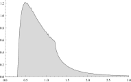
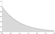
Figure 1. Asymptotic spacing distribution for $\mathbb{Z}^{2}$ (left) and Poisson (right).

The graphs in Figure 1 were produced by numerical evaluation, using $N\approx 1.98\cdot 10^{6}$ angles in the $\mathbb{Z}^{2}$ lattice case (radius ${r=2900}$), and $N\approx 1.96\cdot 10^{6}$ angles in the Poisson case. The analytic density functions perfectly match the graphs, which gives a hint at how large the amount of samples has to be in general to produce appropriate approximations.
Our interest now is to study other point sets and to check how they fit into this picture. Can one expect some kind of interpolation behaviour between the two reference densities? The primary focus will be on vertex sets coming from aperiodic tilings, since these feature both a repetitive structure but also disorder. In terms of density functions, one might then expect some “mixture” of the $\mathbb{Z}^{2}$ and the Poisson case.
We point out that the existence of a limit distribution is known in the two reference cases. In all other considered cases, we assume that the distribution exists, which is plausible from the numerics. A first step to prove this is given in [19, Thm. A.1]. Since the release of the article’s preprint, further results [20] became available, wherefore we now know the existence of the distribution for regular model sets.

4. Numerical approach

As mentioned in Sec. 3.1, the analytic approach for the integer lattice case is based on the theory of Farey fractions. This framework does not extend properly to arbitrary locally finite point sets. And even for subsets of $\mathbb{Z}$-modules (like all our covered examples are), this fails since the key property, the closed description for neighbouring fractions mentioned in 3.1, does not hold anymore – or at least not in an obvious way. One would first need to extend the notion of Farey fraction in a well-defined manner to $\mathbb{Z}$-modules, but even then it is still unclear whether the approach presented in [8] carries over.
From this perspective, an initial approach through numerical methods was chosen. The basic idea is to generate a large list of vertices such that the list needs only a minimal amount of trimming to have a circular shape. Since our focus is on aperiodic tilings, the primary step consisted in creating large patches of these, from which we could then extract the vertex sets with the required properties. The trimming is unavoidable since both feasible methods introduce restrictions on the shape of the generated patch.
There are essentially three methods to produce aperiodic tilings of the plane. The first one is by defining a set of prototiles with matching rules. This method is not suitable for the purpose of implementation. We therefore focus on the alternatives, namely inflation and projection.

4.1. Inflation rules

Probably the most prominent method is via inflation of prototiles. For example, the Tübingen triangle tiling (abbreviated as TT) is produced from two prototiles [3, Ch. 6.2], both with edge length ratio ${\tau:1}$. Here, $\tau$ is the golden mean, which also serves as the inflation factor. The first tile, denoted as type A, is inflated according to the scheme shown in Fig. 2 (rescaled version indicated in red)

$\xrightarrow{\hskip 38.74988pt}$   

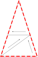
Figure 2. Tile A maps to 2$\times$A and 1$\times$B.

while type B follows the rule shown in Fig. 3.

$\xrightarrow{\hskip 38.74988pt}$   

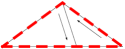
Figure 3. Tile B maps to 1$\times$A and 1$\times$B.

One can see from the rules that the prototiles appear in both chiralities in the resulting tiling. The reflected tiles are simply inflated via the reflected rules.
It can be shown that, for properly chosen edge lengths, the resulting vertex set lives in $\mathbb{Z}[\zeta_{5}]$ with ${\zeta_{n}:=\exp(2\pi i/n)}$ a primitive $n$-th root of unity. The first step, however, is to generate the tiling patch itself and afterwards to extract the vertices. We start with one of the prototiles and apply the inflation rule a few times, inspecting the result for symmetric subpatches in each step. In this case, the inflation rule applied to one prototile of type A produces the patch shown in Fig. 4 (subpatch shaded in grey):

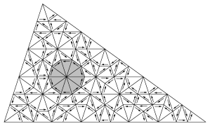
Figure 4. Patch produced from five inflation steps applied to the TT prototile A.

Now, one can isolate the indicated subpatch and use it as initial patch for the inflation. From the computational point of view, this imposes some difficulties. We formulate these for general modules $\mathbb{Z}[\zeta_{n}]$, while keeping in mind the example of the TT tiling (${n=5}$) for illustrative purposes.

1. Inflation steps are applied iteratively. This quickly leads to accumulation of numerical errors. To avoid this, we solely employ integer arithmetic and only switch to floating-point when computing the angular component $\arctan(y/x)$ of a vertex $(x,y)$.

2. Elements of $\mathbb{Z}[\zeta_{n}]$ need to be encoded exactly. These types of $\mathbb{Z}$-modules can be written as

   $$\hskip 34.44434pt\mathbb{Z}[\zeta_{n}]\;=\;\{a_{0}+a_{1}\zeta_{n}+\ldots+a_{r-1}\zeta_{n}^{r-1}\;:\;a_{i}\in\mathbb{Z}\}$$

   ($r=\phi(n)$ the Euler totient function) and therefore only require $r$ integers to encode one element (resulting in a vertex size of $4\times 4=16$ bytes for the TT if one uses standard $32$-bit integers). The vertex byte count is in fact significant, see point (-1pt5-1pt).

3. The inflation rule applies to prototile objects, so we have to keep a tile list during the patch construction. Because of (-1pt1-1pt), we want an exact encoding for list elements. We represent a tile using the type (A/B for TT), the chirality (not always needed), a reference point of the tile (exact in the $\mathbb{Z}$-module case, see (-1pt2-1pt) above) and a rotation of the tile around the reference point. This requires a quantisable angle (the tile is only allowed to appear with a finite number of distinct rotations), which fails when one considers for example the famous pinwheel tiling [23].

   Table 1. Prototile bit encoding for the TT tiling.

   property	states	bit count
   type	A / B	$1$
   chirality	normal / mirrored	$1$
   reference	–	$4\cdot 32$ ($=16$ bytes)
   rotation	$\{0,\ldots,9\}$	$4$

4. The prototile description is only helpful while growing the patch, but becomes cumbersome as soon as one is interested in raw vertex data. Each prototile object decomposes into a bunch of vertices (three for the TT). Applying a decomposition step to each prototile in the output list yields a list with many duplicate vertices, requiring an additional step to reduce the list to unique vertices. This involves constantly accessing the list to locate already present vertices, making it preferrable to have a low element byte count.

5. The determination of visibility of a single vertex is generally very different from the $\mathbb{Z}^{2}$-case, where the test consisted of computing the $\gcd$ of the two coordinates. In the generic case, we have to consider the whole set of unique vertices to determine the visibility of one vertex by doing a geometric ray test (see Eq. (2.1)). It proved to be more efficient to combine the removal pass for unique vertices with the visibility test pass and to use custom data structures to further speed up the process.

The computation time mentioned in (-1pt5-1pt), which is $\mathcal{O}(n)$, is not to be underestimated ($n$ being the total amount of vertices collected at some point), and led to the investigation of cases with tests having similar complexity as $\mathbb{Z}^{2}$, which is just $\mathcal{O}(1)$.
To summarise, there are roughly three steps: Growing a large circular patch, removal of duplicate vertices together with the visibility test, and finally mapping vertices to angles followed by proper normalisation.
A simple optimisation consists of removing redundancy imposed by symmetry of the input set. For example, the $\gcd$ is fixed under sign changes of the parameters. It also is $D_{4}$-symmetric, wherefore it suffices to consider the halved upper-right quadrant of the $\mathbb{Z}^{2}$ lattice.

4.2. Model set description / cut-and-project

A different method for constructing tilings is given by the cut-and-project method. The advantage is that it directly yields vertices of the tiling and does not require keeping track of the adjacency information. Another reason for choosing this description, if applicable, is that some configurations admit a much easier condition to determine visibility of a given vertex by using local information only. In this regard, such cases are very similar to $\mathbb{Z}^{2}$ together with the $\gcd$-test.
In a simplified setting, let $(\mathbb{R}^{d},\mathbb{R}^{k},\mathcal{L})$ be a triple and $\pi,\pi_{\operatorname{int}}$ projections satisfying the following conditions:

1. $\mathcal{L}$ is a lattice in $\mathbb{R}^{d}\times\mathbb{R}^{k}$;

2. $\pi:\mathbb{R}^{d}\times\mathbb{R}^{k}\rightarrow\mathbb{R}^{d}$, with $\pi|_{\mathcal{L}}$ injective;

3. $\pi_{\operatorname{int}}:\mathbb{R}^{d}\times\mathbb{R}^{k}\rightarrow\mathbb{R}^{k}$, with $\pi_{\operatorname{int}}(\mathcal{L})\subset\mathbb{R}^{k}$ dense.

This setup is called a cut-and-project scheme (CPS). If we define $L:=\pi(\mathcal{L})$, the conditions above induce ${\star:L\rightarrow\mathbb{R}^{k}}$, the star map. The lattice can then be written as $\mathcal{L}={\{(x,x^{\star}):x\in L\}}$ and one usually encodes the CPS in a diagram. The right hand side in Figure 5 describes the internal space, the left one the physical space (since this is where the point set of the tiling itself lives).

Figure 5. General case of a $\mathbb{R}$-CPS.

Details about the generic definition can be found in [24, 3]. Given a CPS as defined above, a model set then arises from choosing a subset $W\subseteq\mathbb{R}^{k}$ (with certain conditions) and considering the set

$$\mbox{\Large$\curlywedge$}(W)\;:=\;\{x\in L\;:\;x^{\star}\in W\}\text{.}$$

The subset $W$ is called the window of the model set (also denoted as acceptance region or occupation domain). It can be shown that point sets of certain aperiodic tilings can be generated using this description. This is also the important aspect for our implementation purpose, since the main work now consists of generating a suitable “cutout” ${L_{0}\subset L}$ and then applying the window condition ${x^{\star}\in W}$ to each ${x\in L_{0}}$.
Since generic model sets are a broad topic, we restrict ourself to a more manageable subclass in the next section. It should also be emphasised that we only consider model sets with physical space $\mathbb{R}^{2}$, for reasons pointed out before.

4.3. Histogram statistics

It seems natural to compute statistical data (like variance and skewness) to analyse the histogram data. We choose not to do so, since this can be misleading. One can see from the explicit density function $g(t)$ of the $\mathbb{Z}^{2}$ case in Sec. 3.1 that the moments of order ${k\geq 2}$ fail to exist. A Taylor expansion gives

$$g(1/t)=\frac{36}{\pi^{4}}t^{3}+\frac{162}{\pi^{6}}t^{4}+\mathcal{O}(t^{5})\;\text{ for }\;t\rightarrow 0_{+}\;\text{,}$$

characterising the decay behaviour of the tail. Instead of the statistics, which just exist because of finite size effects, we provide the coefficients $c_{k}$ of $t^{k}$ (usually two) when the tail of the respective histogram can be fitted with a power law.

5. Cyclotomic model sets

As stated above, we are interested in model set configurations which admit local visibility tests. This special case is given by the planar cyclotomic model sets of order ${n\in\mathbb{N}}$. It corresponds to choosing ${d=2}$, ${k=\phi(n)-2}$ and $L=\mathbb{Z}[\zeta_{n}]$ in Figure 5. Since $\mathbb{Z}[\zeta_{n}]=\mathbb{Z}[\zeta_{2n}]$ for $n$ odd, we impose the condition $n\not\equiv 2$ mod $4$; compare [3, Ch. 3.4].
The setting can now be used to generate $n$-fold (rotationally) symmetric point sets (and tilings). The $\star$-map, which maps from physical to internal space, is given by the extension of an algebraic conjugation; see [3] for details.
Since the cases ${n=3,4}$ yield a planar lattice, we only consider the configurations with ${n\geq 5}$. Of particular interest are integers $n$ which admit a simple window test. There are three unique cases where the window lives in $\mathbb{R}^{2}$, or stated differently where ${\phi(n)=4}$ holds: 5, 8 and 12.

input : maxsteps, initpoint

output : vertexlist

initialize vertexlist and add initpoint;

for step $\leftarrow$ $1$ to maxsteps do

       foreach $\text{p}\in\text{vertexlist}$ do

            

            for $k\leftarrow 0$ to ${n-1}$ do

                   pp $\leftarrow$ p + $\zeta_{n}^{k}$;

                  

                  if pp is already in vertexlist then

                         skip;

                        

                   if $\text{pp}^{\star}$ not in window then

                         skip;

                        

                  

                  add pp to vertexlist;

                  

             end for

            

       end foreach

      

end for

Algorithm 1 Patch generation for the cyclotomic case.

The pseudo code in Algorithm 1 then produces the vertices of a $k$-gon-shaped ($k\in\{10,8,12\}$) patch of the corresponding tiling. Note that for $n=5$, the shape is $10$-fold symmetric because of the $n\not\equiv 2$ (see above) condition. This $k$-gon shape is desirable because it is already close to being circular and needs just minor trimming.

5.1. Ammann–Beenker tiling

We employ the Ammann–Beenker (AB) tiling in its classic version [1, 3] with a triangle and a rhombus. It admits a stone inflation (essentially a rule which can be implemented as blowing up the tile followed by a dissection process), where the triangle (here called the prototile of type A) is inflated as given below in Figure 6:

$\xrightarrow{\hskip 38.74988pt}$   

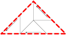
Figure 6. Tile A maps to 3$\times$A and 2$\times$B.

The triangle appears in the tiling with both chiralities, and the other chirality just uses the reflected rule. The rhombus (prototile of type B) appears without chirality and is inflated according to the rule in Figure 7.

$\xrightarrow{\hskip 38.74988pt}$   

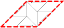
Figure 7. Tile B maps to 4$\times$A and 3$\times$B.

Here, the inflation multiplier is given by the silver mean $\lambda_{\text{sm}}=1+\sqrt{2}$, which is a Pisot-Vijayaraghavan (PV) unit. PV numbers are algebraic integers ${\lambda>1}$ such that all algebraic conjugates (except for $\lambda$ itself) lie in the open unit disk. There is a relation between the regularity of the tiling and the properties of the inflation multiplier. PV inflations seem to admit more regular tiling structures [3, Ch. 2.5]; compare Sec. 6 for an example of a less regular tiling point set.
A nice property of the AB tiling is that it can be described as a cyclotomic model set [3, Ex. 7.8]. It corresponds to the diagram in Figure 5 of cyclotomic type with parameter ${n=8}$. The tiling vertices can therefore be described as the set

$$T_{\textsf{AB}}=\{x\in\mathbb{Z}[\zeta_{8}]\;:\;x^{\star}\in W_{8}\}\text{,}$$

where the $\star$-map is given by the extension of $\zeta_{8}\mapsto\zeta_{8}^{3}$ and the window $W_{8}$ is a regular octagon centered at the origin (edge length one, see Figure 8 for the orientation).

The maximal real subring of $\mathbb{Z}[\zeta_{8}]$ is $\mathbb{Z}[\sqrt{2}]$, with the unit group generated by ${\pm\lambda_{\text{sm}}}$ from above. By inspecting the action of these units on the elements of the $\mathbb{Z}$-module, one can derive a local visibility test

$$V_{\textsf{AB}}=\{x\in T_{\textsf{AB}}\;:\;\lambda_{\text{sm}}x^{\star}\notin W_{8}\text{ and }x\text{ is coprime}\}$$

for the reference point chosen as the origin. By coprimality of $x$ we mean coprimality of the coordinates in the direct-sum representation

$$\mathbb{Z}[\zeta_{8}]\;=\;\mathbb{Z}[\sqrt{2}]\oplus\mathbb{Z}[\sqrt{2}]\cdot\zeta_{8}\;\text{.}$$

Consider an element $x_{1}+x_{2}\cdot\zeta_{8}$ in the above decomposition. The module $\mathbb{Z}[\sqrt{2}]$ is a Euclidean domain and therefore admits an algorithm to compute the $\mathbb{Z}[\sqrt{2}]$-gcd of $x_{1}$ and $x_{2}$. By coprime we then understand that this gcd $y$ is a unit, which is equivalent to $\lvert\operatorname{N}(y)\rvert=1$, with $\operatorname{N}$ the algebraic norm in the corresponding module, here given by the map $\operatorname{N}(a+b\cdot\sqrt{2})=a^{2}-2\cdot b^{2}$.

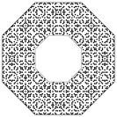
Figure 8. Visible vertices of the $8$-fold symmetric Ammann–Beenker tiling
(left: direct space, right: internal space).

The first part of the visibility condition ${x^{\star}\in W_{8}}$ translates to the following geometric condition in internal space: If a vertex is visible, then it lives on a belt in internal space, which results from cutting out a scaled down version of the window from the original window. Both windows are indicated on the right hand side of Figure 8.

Table 2. Visibility statistics for the symmetric Ammann–Beenker tiling.

maxsteps	vertices	visible	percentage
40	561	327	58.2%
400	47713	27561	57.7%
1500	662265	382221	57.7%
2500	1835941	1059753	57.7%

We see that the histogram (generated from roughly $1.8\cdot 10^{6}$ vertices) features several characteristics which we have already observed for the $\mathbb{Z}^{2}$-case: A pronounced gap is present where the distribution has zero mass; then, we have a middle section where the bulk of the mass is concentrated, and finally a tail section with a power law decay.

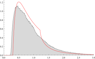
Figure 9. Distribution of the radial spacings of a large $D_{8}$-symmetric AB patch.

For an overview of the histogram statistics, see Table 3 at the end of Sec. 5.

5.2. Tübingen triangle tiling

The Tübingen triangle tiling (TT) is a decagonal case of a cyclotomic model set with planar window (see [6, 5] and [3, Ex. 7.10]). The underlying module is $\mathbb{Z}[\zeta_{5}]$ with maximal real subring $\mathbb{Z}[\tau]$, where $\tau$ is again the multiplier for the corresponding inflation rule (see Figure 2 and 3). See below for a circular patch generated from applying the inflation rule four times:

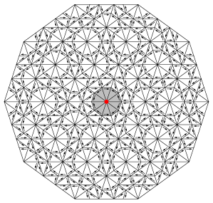
Figure 10. Patch of the Tübingen triangle tiling (after 4 inflations of the central patch)

For the computation of the vertices used for the radial projection, again the model set description

$$T_{\textsf{TT}}\;=\;\{x\in\mathbb{Z}[\zeta_{5}]\;:\;x^{\star}\in W_{10}+\epsilon\}$$

was employed. The window $W_{10}$ is a decagon with edge length $\sqrt{(\tau+2)/5}$, and like the AB window, the right-most edge is perpendicular to the $x$-axis. Here, the $\star$-map is the extension of $\zeta_{5}\mapsto\zeta_{5}^{2}$. In this case, we need to apply a small generic shift $\epsilon$ to the window, otherwise leading to singular vertices (vertices which lie on the boundary of the window when projected to internal space). These are difficult to handle because of precision issues when testing on the boundary. We therefore restrict ourself to non-singular sets. In our case we use $\epsilon=10^{-4}\cdot(1,1)$ as the shift. The important aspect here is not to shift in the direction of the window edges. Similar to the eightfold case, a local visibility condition

$$V_{\textsf{TT}}\;=\;\{x\in T_{\textsf{TT}}\;:\;\tau x^{\star}\notin W_{10}-\epsilon\text{ and }x\text{ is coprime}\}$$

can be derived. The direct-sum represention here is $\mathbb{Z}[\zeta_{5}]=\mathbb{Z}[\tau]\oplus\mathbb{Z}[\tau]\cdot\zeta_{5}$, and $\mathbb{Z}[\tau]$ is again Euclidean.
Evaluation with a large patch ($\approx 1.5\cdot 10^{6}$ vertices) produces the following histogram:

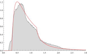
Figure 11. Spacing distribution of a large Tübingen triangle patch.

While being similar to the AB histogram in overall shape, there are numerous differences in detail, especially in the middle section, which features a lot more structure and is also nicely aligned to the $\mathbb{Z}^{2}$ density function.
Zooming into the gap area might even suggest that the middle section decomposes into smaller components (first step: $(0.18,0.3)$, second step: $(0.3,0.5)$, third step: $(0.5,1.3)$).

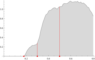
Figure 12. Zoom into the bulk of the Tübingen triangle distribution.

Again, the statistics can be found in Table 3 below.
A related example of a distribution in closed form, for the golden L (which is not a tiling system), has recently been described by Athreya et al. [2]. It bears strong resemblence with Fig. 11, thus making it fall into our “ordered regime”. This supports the existence of universal features in this approach.

5.3. Gähler’s shield tiling

The Gähler shield (GS) tiling [12, Ch. 5] is our last cyclotomic model set with internal space $\mathbb{R}^{2}$. It uses a dodecagonal configuration [3, Ex. 7.12] and is also interesting in its algebraic properties, which make the visibility test slightly more involved. The vertex set is

$$T_{\textsf{GS}}\;=\;\{x\in\mathbb{Z}[\zeta_{12}]\;:\;x^{\star}\in W_{12}+\epsilon\}$$

with the $\star$-map defined by $\zeta_{12}\mapsto\zeta_{12}^{5}$. The window $W_{12}$ is a dodecagon with edge length one and the usual orientation. Again, a shift has to be applied to avoid singular vertices. The underlying $\mathbb{Z}$-module decomposes into

$$\mathbb{Z}[\sqrt{3}]\oplus\mathbb{Z}[\sqrt{3}]\cdot\zeta_{12}\;\text{ with }\;\lambda_{12}:=2+\sqrt{3}$$

generating the unit group of $\mathbb{Z}[\sqrt{3}]$.
The local visibility test behaves in a more complex fashion here. Consider an $x\in\mathbb{Z}[\zeta_{12}]$ and denote by $\operatorname{N}$ the algebraic norm of $\mathbb{Z}[\sqrt{3}]$. Now write $x$ in the direct-sum decomposition $x=x_{1}+x_{2}\cdot\zeta_{12}$ and define the map

$$n:\mathbb{Z}[\zeta_{12}]\rightarrow\mathbb{N}_{1}\;\text{ via }\;x\mapsto\lvert N(\gcd(x_{1},x_{2}))\rvert\text{.}$$

Within our finite patch $P$, the set of visible points can then be described as

$$V_{\textsf{GS}}\;=\; \{x\in T_{\textsf{GS}}\;:\;n(x)=1\wedge\lambda_{1}x^{\star}\notin W_{12}+\epsilon\}\cup{}$$

$$\{x\in T_{\textsf{GS}}\;:\;n(x)=2\wedge\lambda_{2}x^{\star}\notin W_{12}-\epsilon\}\;\text{,}$$

where $\lambda_{1}:=\sqrt{\lambda_{12}\cdot 2}$ and $\lambda_{2}:=\sqrt{\lambda_{12}/2}$ (therefore $\lambda_{1}\cdot\lambda_{2}=\lambda_{12}$), and as long as $\epsilon$ is small enough in relation to the distances within $P^{\star}$. The first set-component of $V_{\textsf{GS}}$ is again comprised of coprime elements. The second set, however, is exceptional, and its existence is linked to the degree of the underlying cyclotomic field, which is ${n=12}$ here – a composite number instead of a prime power as in the other two cases (for cyclotomic fields see [25]). The difficulty can also be seen on the level of $\mathbb{Q}(\zeta_{n})$, where the unit group is slightly larger than in the prime power cases, here enlarged by an additional generating element $z=\sqrt{2+\sqrt{3}}\cdot\zeta_{24}$.

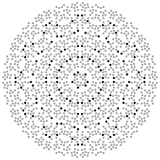
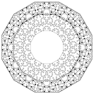
Figure 13. Visible vertices of a GS tiling
(left: direct space, right: internal space).

We can see on the right hand side of Figure 13 that two belts develop in internal space, one for the coprime vertices and another one for the exceptional ones. Coprime vertices are represented as grey dots and exceptional vertices as black dots. The boundaries of the rescaled (with the factors $\lambda_{1}$ and $\lambda_{2}$ respectively) windows use the same coloring.

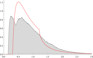
Figure 14. Spacing distribution of a large patch of the Gähler shield tiling.

While still retaining the known three-fold structure of the two other cases, the GS tiling seems to approach the slope-like characteristic from the Poisson case.

Table 3. Statistical data generated from the radial projection (mean is always $1.0$).

tiling	gap size	$c_{3}$	$c_{4}$	$e$	$k$
$\mathbb{Z}^{2}$	0.304	0.369	0.168	—	—
AB	0.222	0.248	0.496	2.79	38560
TT	0.182	0.239	0.513	2.60	31376
GS	0.152	0.232	0.547	4.75	67524

The power law fitting was done for the tail starting at $3.0$ (see Sec. 4.3 for definitions). We indicate the quadratic error by $e$ in units of $10^{-10}$ and the amount of data points by $k$.

6. A non-Pisot inflation

We have seen that the examples of Sec. 5 are qualitatively close to the order properties of the $\mathbb{Z}^{2}$ lattice. A similar behaviour of cyclotomic model sets can also be seen in the mildly related case of discrete tomography [15]. One might guess that all kind of deterministic aperiodic tilings behave that way. However, it turns out that this is not the case.
The chiral Lançon–Billard (LB) tiling [16] is an example of an inflation-based tiling with a non-PV multiplier given by

$$\lambda_{\textsf{LB}}\;=\;\sqrt{\frac{1}{2}\big{(}5+\sqrt{5}\big{)}}\;\text{.}$$

The inflation rule applies to two rhombic prototiles (see Fig. 15 and Fig. 16).

$\xrightarrow{\hskip 25.83325pt}$   

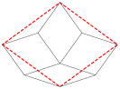
Figure 15. Tile A maps to 3$\times$A and 1$\times$B.

The resulting tiling vertices live in $\mathbb{Z}[\zeta_{5}]$ (see [3, Ch. 6.5.1] for details, also concerning the non-PV property of $\lambda_{\textsf{LB}}$), like the Tübingen triangle tiling above.

$\xrightarrow{\hskip 25.83325pt}$   

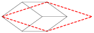
Figure 16. Tile B maps to 1$\times$A and 2$\times$B.

The LB tiling admits no model set description and it fails to be a stone inflation, as one can see from the above rules.
By multiple inflation of tile A, one can isolate a legal patch of circular shape that is comprised of five tiles of type A. We use this patch as our initial seed to grow suitable patches.

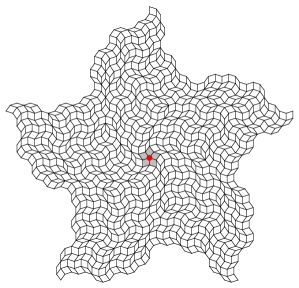
Figure 17. Fivefold symmetric patch of the chiral LB tiling (after 4 inflations of the initial patch).

The resulting patches are $C_{5}$ symmetric and begin to show a high amount of spatial fluctuation when increasing the number of inflation steps (the histogram in Figure 18 was computed after applying $12$ inflations).

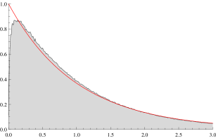
Figure 18. Spacing distribution of a large patch of the Lançon–Billard tiling.

While not exactly matching the exponential distribution from the Poisson case, the radial projection at least is sensitive to the higher amount of spatial disorder in this tiling. In particular, it shows an exponential rather than a power law decay for large spacings. For the histogram statistics, see Table 4 below.

7. Other planar tilings

The tilings considered in Secs. 5 and 6 indicate that the method gives at least partial information about the order of the point set. Let us look at some more examples.
The chair tiling [13] is an example of a inflation tiling with integer multiplier. It works with just one L-shaped prototile and can produce patches with $D_{4}$ symmetry.
The patches can also be described as model sets [3], but with a more complicated internal space. We thus employ the inflation method here.

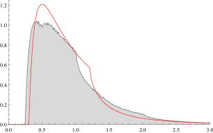
Figure 19. Spacing distribution of a large patch of the chair tiling.

The vertex set is a subset of $\mathbb{Z}^{2}$. It gives a good example why one has to be careful with the visibility test. Although the set lives in $\mathbb{Z}^{2}$, the standard $\gcd$-test fails in this situation. Consider a vertex ${p:=(x,y)}$ which is not coprime, say with $\gcd(x,y)=k>1$. For the integer lattice, one knows that ${p_{0}:=(\frac{x}{k},\frac{y}{k})}$ is an element of the set and therefore occludes $p$. This does not need to be the case here and Figure 20 shows that the difference is indeed significant.

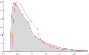
Figure 20. Spacing distribution of a large patch of the chair tiling (using the standard gcd visibility test).

The Penrose–Robinson (PR) tiling is similar to the TT on the level of the inflation rule. It uses the same prototiles, but a different dissection rule [3, Ch. 6.2] after blowing up the tiles by the inflation factor $\tau$.

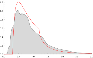
Figure 21. Spacing distribution of a large patch of the Penrose–Robinson tiling.

Even though it shares these features with the TT, the resulting distribution is rather different and offers a high amount of structure in the bulk section, which can be identified as plateau-like increments.

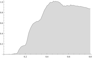
Figure 22. Zoom into the bulk of the PR distribution.

Another tiling of Penrose-type can again be implemented by using a model set description. This rhombic Penrose (RP) tiling [5] is special in that it uses a multi-window configuration [3, Ex. 7.11]. Here, the CPS in Figure 5 is fixed, but multiple windows $W_{i}$ are used. Define the homomorphism

$$\kappa:\mathbb{Z}[\zeta_{5}]\rightarrow\mathbb{Z}/5\mathbb{Z}\quad\text{ by }\quad\kappa(\sum_{i}{c_{i}\zeta_{5}^{i}})=\sum_{i}{c_{i}}\mod 5,$$

then the window $W_{i}$ for which the vertex $x\in\mathbb{Z}[\zeta_{5}]$ is tested, is chosen depending on $\kappa(x)$.

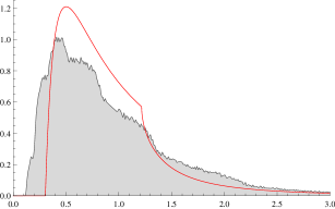
Figure 23. Spacing distribution of a large patch of the rhombic Penrose tiling.

However, the patches for this case had to be generated using the geometric visibility test. Although the vertices coming from different $W_{i}$ are disjoint, there is still occlusion between the sets which renders the local test ineffective in this setup.

Table 4. Statistical data for the other considered tilings ($e$ is the error term).

tiling	gap size	$c_{3}$	$c_{4}$	$c_{5}$	$e$
LB	0.0030	—	—	—	—
chair	0.2536	0.229	0.538	—	$5.07\cdot 10^{-10}$
PR	0.0783	0.066	1.339	—	$1.81\cdot 10^{-10}$
RP	0.1169	0.459	-2.432	8.395	$1.41\cdot 10^{-9}$

For the fit of the RP tiling, an additional power was used, to achieve a similarly small error as in the other cases. Also, a logarithmic fit provides numerical evidence that the decay behaviour of the chiral LB tiling is identical to the Poisson case.
Another aspect, which is numerically plausible, is the continuous dependence of the spacing distribution of the cyclotomic cases (Sec. 5) under small perturbations of the window which leave the area fixed. Replacing the window with a circle of the same area does not have any noticeable influence on the histogram. This is in line with related continuity results in [20] and certainly a much stronger property than the invariance under removal of singular vertices (see Sec. 5.2), which are known to have density zero in the limit.

8. Concluding remarks

It would be interesting to study tilings which feature even higher rotational symmetry than the examples we considered here. While the data gathered from the three simple cyclotomic cases already shows a tendency, more tilings are needed to fill the picture. The de Bruijn method [11] via dualisation of a grid appears to be a suitable candidate to generate these kind of tilings.
Another aspect which needs further investigation is the existence of a gap in all studied cases, except the LB one. For cyclotomic model sets, this seems to be related to the existence of lines with high density of points on them [21]. This is a feature that is shared with the $\mathbb{Z}^{2}$ case. This has also been observed in [20].
Also of interest, but still unclear, is an extension of this method to higher dimension. A possible way for $\mathbb{R}^{3}$ would be to again project vertices of our set onto the $3$-dimensional ball of radius $r$. For each projected point $p$, one could now select the neighbour $q$ with minimal distance to $p$ on the sphere and consider the angle of the arc between $p$ and $q$. This again produces a list of angles with which we proceed in the usual way. From a computational point of view, this case is a lot more involved, since it requires an exhaustive search for each projected point to find its neighbour.
Before closing, we want to point out that projecting from a centre of maximal symmetry might seem intuitive at first, but still is kind of special. Since shifting the center indeed changes the distribution, we want to investigate if some averaging (similar to the shelling problem [4] and as also discussed in [20]) makes more sense here.

References

- [1] R. Ammann, B. Grünbaum, and G.C. Shephard. Aperiodic tiles. Discr. & Comput. Geom., 8(1):1–25, 1992.
- [2] J. S. Athreya, J. Chaika, and S. Lelievre. The gap distribution of slopes on the golden L. ArXiv e-prints, August 2013.
- [3] M. Baake and U. Grimm. Aperiodic Order Vol. I: A Mathematical Invitation. Cambridge University Press, Cambridge, 2013.
- [4] M. Baake, U. Grimm, D. Joseph, and P. Repetowicz. Averaged shelling for quasicrystals. Mat. Sci. Eng. A, 294-296:441–445, 2000.
- [5] M. Baake, P. Kramer, M. Schlottmann, and D. Zeidler. Planar patterns with fivefold symmetry as sections of periodic structures in -space. J. Mod. Phys. B, 4(15-16):2217–2268, 1990.
- [6] M. Baake, P. Kramer, M. Schlottmann, and D. Zeidler. The triangle pattern – a new quasiperiodic tiling with fivefold symmetry. Mod. Phys. Lett. B, 4(4):249–258, 1990.
- [7] M. Baake, R. V. Moody, and P. A. B. Pleasants. Diffraction from visible lattice points and th power free integers. Discrete Math., 221(1-3):3–42, 2000.
- [8] F. P. Boca, C. Cobeli, and A. Zaharescu. Distribution of lattice points visible from the origin. Commun. Math. Phys., 213(2):433–470, 2000.
- [9] C. Cobeli and A. Zaharescu. The Haros-Farey sequence at two hundred years. Acta Univ. Apulensis. Math. - Inform., 5:1–38, 2003.
- [10] J. M. Cowley. Diffraction Physics. North-Holland. Amsterdam, 3rd edition, 1995.
- [11] N. G. de Bruijn. Algebraic theory of Penrose’s nonperiodic tilings of the plane. I, II. Nederl. Akad. Wetensch. Indag. Math., 43(1):39–52, 53–66, 1981.
- [12] F. Gähler. Quasicrystal Structures from the Crystallograhic Viewpoint. PhD thesis no. 8414, ETH Zürich, 1988.
- [13] B. Grünbaum and G. C. Shephard. Tilings and Patterns. Freeman, New York, 1987.
- [14] A. Hof. On diffraction by aperiodic structures. Commun. Math. Phys., 169:25–43, 1995.
- [15] C. Huck and M. Spiess. Solution of a uniqueness problem in the discrete tomography of algebraic delone sets. J. reine angew. Math. (Crelle), 677:199–224, 2013.
- [16] F. Lançon and L. Billard. Two-dimensional system with a quasi-crystalline ground state. J. Phys. France, 49(2):249–256, 1988.
- [17] E. Landau and J. Franel. Les suites de farey et le problème des nombres premiers. Gött. Nachr., pages 202–206, 1924.
- [18] J. Marklof and A. Strömbergsson. The distribution of free path lengths in the periodic Lorentz gas and related lattice point problems. Ann. of Math. (2), 172(3):1949–2033, 2010.
- [19] J. Marklof and A. Strömbergsson. Free path lengths in quasicrystals. ArXiv e-prints, April 2013.
- [20] J. Marklof and A. Strömbergsson. Visibility and directions in quasicrystals. ArXiv e-prints, April 2014.
- [21] P. A. B. Pleasants. Lines and planes in 2- and 3-dimensional quasicrystals. In Coverings of Discrete Quasiperiodic Sets, Eds. Kramer and Papadopolos, pages 185–225. Springer, Berlin, 2003.
- [22] P. A. B. Pleasants and C. Huck. Entropy and diffraction of the -free points in -dimensional lattices. Discrete Comput. Geom., 50(1):39–68, 2013.
- [23] C. Radin. Miles of Tiles. Amer. Math. Soc., Providence, RI, 1999.
- [24] M. Schlottmann. Cut-and-project sets in locally compact abelian groups. In Quasicrystals and Discrete Geometry, Ed. J. Patera, pages 247–264. Amer. Math. Soc., Providence, RI, 1998.
- [25] L. C. Washington. Introduction to Cyclotomic Fields. Springer, New York, 1997.