First X-ray-Based Statistical Tests for Clumpy-Torus Models: Eclipse Events from 230 Years of Monitoring of Seyfert AGN

Abstract

We present an analysis of multi-timescale variability in line-of-sight X-ray absorbing gas as a function of optical classification in a large sample of Seyfert active galactic nuclei (AGN) to derive the first X-ray statistical constraints for clumpy-torus models. We systematically search for discrete absorption events in the vast archive of Rossi X-ray timing Explorer monitoring of dozens of nearby type I and Compton-thin type II AGN. We are sensitive to discrete absorption events due to clouds of full-covering, neutral or mildly ionized gas with columns $\ga 10^{22-25}$ cm^-2 transiting the line of sight.

We detect 12 eclipse events in 8 objects, roughly tripling the number previously published from this archive. Peak column densities span $\sim 4-26\times 10^{22}$ cm^-2, i.e., there are no full-covering Compton-thick events in our sample. Event durations span hours to months. The column density profile for an eclipsing cloud in NGC 3783 is doubly spiked, possibly indicating a cloud that is being tidally sheared.

We infer the clouds’ distances from the black hole to span $\sim 0.3-140\times 10^{4}R_{\rm g}$. In seven objects, the clouds’ distances are commensurate with the outer portions of Broad Line Regions (BLR), or outside the BLR by factors up to $\sim 10$ (the inner regions of infrared-emitting dusty tori). We discuss implications for cloud distributions in the context of clumpy-torus models. Eight monitored type II AGN show X-ray absorption that is consistent with being constant over timescales from 0.6 to 8.4 yr. This can either be explained by a homogeneous medium, or by X-ray-absorbing clouds that each have $N_{\rm H}\ll 10^{22}$ cm^-2. The probability of observing a source undergoing an absorption event, independent of constant absorption due to non-clumpy material, is $0.006^{+0.160}_{-0.003}$ for type Is and $0.110^{+0.461}_{-0.071}$ for type IIs.

1 INTRODUCTION

While it is generally accepted that active galactic nuclei (AGN) are powered by accretion of gas on to supermassive ($10^{6-9}\rm M_{\odot}$) black holes, the exact geometry and mechanisms by which material gets funneled from radii of kpc/hundreds of pc down to the accretion disk at sub-pc scales remains unclear. This unsolved question is, however, linked to the overall efficiency of how supermassive black holes are fed and to AGN duty cycles.

Clues to the morphology of the circumnuclear gas come from different studies across the electromagnetic spectrum. For instance, Seyfert AGN are generally classified into two broad categories based on the detection or lack of broad optical/UV emission lines (type I or II, respectively), with intermediate subclasses (1.2, 1.5, 1.8, 1.9) depending on broad lines’ strengths (e.g., Osterbrock 1981). Unification theory posits that all Seyferts host the same central engine, but observed properties depend on orientation due to the presence of dusty circumnuclear gas blocking the line of sight to the central illuminating source in type II Seyferts. The classical model holds that a primary component of this obscuring gas is a pc-scale, equatorial, dusty torus (Antonucci & Miller 1985; Urry & Padovani 1995), where “torus” generally denotes a donut-shaped morphology, supplying the accretion disk lying co-aligned inside it. However, some recent papers (e.g., Pott et al. 2010) use the term “torus” to denote simply the region where circumnuclear gas can exist, with the precise morphology of that region still to be determined; we adopt that notation in this paper.

A donut morphology can explain the observed bi-conical morphology of Narrow Line Regions (NLR), e.g., via collimation of ionizing radiation (e.g., Evans et al. 1994), and also why most type II Seyferts show evidence for X-ray obscuration along the line of sight. However, the relation between optical/UV-reddening dust and X-ray absorbing gas is not straightforward. Very roughly 5 per cent of all AGN have differing X-ray and optical obscuration indicators (e.g., X-ray-absorbed type Is, Perola et al. 2004; Garcet et al. 2007); a complication is that optical obscuration probes only dusty gas, while X-ray absorption probes both dusty and dust-free gas, and X-ray columns can exceed inferred optical-reddening columns by factors of 3–100 (Maiolino et al. 2001). Lutz et al. (2004) and Horst et al. (2006) demonstrated that the infrared (IR) emission by dust, which thermally re-radiates higher energy radiation, is isotropic, with type I and II Seyferts having similar ratios of X-ray to mid-IR luminosity. This is not expected from classical unification models, since the classical donut-shaped torus both absorbs and re-emits anisotropically. Furthermore, if the torus is comprised of primarily Compton-thick gas, i.e., with X-ray-absorption column densities $N_{\rm H}$ above $1.5\times 10^{24}$ cm^-2, then it is not clear how Compton-thin columns can be attained unless lines of sight happen to “graze” the outer edges. A unification scheme based solely on inclination angle and the presence of a donut-shaped absorbing morphology may thus be an oversimplification (Elvis 2012). It is also not clear how geometrically thick structures (scale heights $H/R\sim 1$) comprised of cold gas (100 K) are supported vertically over long timescales (Krolik & Begelman 1988).

Meanwhile, the community has accumulated observations of variations in the X-ray absorbing column $N_{\rm H}$ in both (optically classified) type Is and IIs, with timescales of variability ranging from hours to years. For instance, Risaliti, Elvis, & Nicastro (2002; hereafter REN02) claim that variations in $N_{\rm H}$ in a sample of X-ray-bright, Compton-thin and moderately Compton-thick type IIs are ubiquitous, with typical variations up to factors of $\sim 1.5-3$. Current X-ray missions such as XMM-Newton, Chandra and Suzaku have enabled high precision studies of variations in $N_{\rm H}$ in numerous AGN; major findings include the following:

$\bullet$ Numerous moderately Compton-thick variations ($\Delta$$N_{\rm H}\sim 10^{23-24}$ cm^-2) on timescales $\la 1-2$ d in NGC 1365 (Risaliti et al. 2005, 2007, 2009a) and ESO 323–G77 (Miniutti et al. 2014); moderately Compton-thick variations on timescales from days to months in NGC 7582 (Bianchi et al. 2009).

$\bullet$ Changes in covering fraction of partial-covering absorbers on timescales from $<$1 d (NGC 4151, Puccetti et al. 2007; NGC 3516, Turner et al. 2008; Mkn 766, Risaliti et al. 2011; SWIFT J2127.4+5654, Sanfrutos et al. 2013) to months–years in NGC 4151 (de Rosa et al.  2007 and Markowitz et al. in preparation, using BeppoSAX and Rossi X-ray Timing Explorer (RXTE) data, respectively).

$\bullet$ Time-resolved spectroscopy of full eclipse events (ingress and egress), yielding constraints on clouds’ density profiles for long-duration (3–6 months) eclipses in NGC 3227 (Lamer et al. 2003) and Cen A (Rivers et al. 2011b) and for eclipses $\la$1 d in NGC 1365 (Maiolino et al. 2010) and SWIFT J2127.4+5654 (Sanfrutos et al. 2013).

These results suggest that the circumnuclear absorbing gas is clumpy, with non-homogeneous or clumpy absorbers being invoked to explain time-variable X-ray absorption as far back as Ariel V and Einstein observations (Barr et al. 1977; Holt et al. 1980). With the concept of a homogeneous, axisymmetric absorber thus under scrutiny, the community has been developing torus models incorporating clumpy gas, e.g., Elitzur & Shlosman (2006) and Nenkova et al. (2008a, 2008b; see Hönig 2013 for a review), although suggestions that the torus should consist of clouds go as far back as, e.g., Krolik & Begelman (1986, 1988). In the most recent models, total line-of-sight absorption for a given source is quantified as a viewing dependent probability based on the size and locations of clouds, although typically, clouds are preferentially distributed towards the equatorial plane. The fraction of obscured sources depends on the average values and distributions of such parameters as the average number of clouds lying along a radial path, and the thickness of the cloud distribution. Clouds are possibly supported vertically by, e.g., radiation pressure (Krolik 2007) or disk winds (Elitzur & Shlosman 2006).

Observations so far suggest that clouds are typically on the order of $10^{13-15}$ cm in diameter, with number densities $\sim 10^{8-11}$ cm^-3. Inferred distances from the black hole, usually based on constraints from X-ray ionization levels and assumption of Keplerian motion, range from light-days and commensurate with clouds in the Broad Line Region (BLR; e.g., for NGC 1365 and SWIFT J2127.4+5654) to several light-months (Rivers et al. 2011b for Cen A) and commensurate with the IR-emitting torus in that object. We emphasize “commensurate,” as X-ray absorbers lie along the line of sight, but BLR clouds likely contain components out of the line of sight.

Recent IR interferometric observations have spatially resolved distributions of dust down to radii of tenths of pc (e.g., Kishimoto et al. 2009, 2011; Tristram et al. 2009; Pott et al. 2010). In addition, there are suggestions from reverberation mapping of the thermal continuum emission in four Seyferts that warm dust gas extends down to $\sim 10-80$ light-days, likely just outside the outer BLR (Suganuma et al. 2006). As suggested by Netzer & Laor (1993), Elitzur (2007), and Gaskell et al. (2008), the BLR and dusty torus may be part of a common radially extended structure, spanning radii inside and outside the dust sublimation radius $R_{\rm d}$, respectively, since dust embedded in the gas outside $R_{\rm d}$ suppresses optical/UV line emission. Optical obscuration is due to dusty gas, while X-ray obscuration can come from dusty or dust-free gas. X-ray obscuration is thus the only way to probe obscuration inside $R_{\rm d}$.

In order to gain a more complete picture of the geometry of circumnuclear gas in AGN, however, the community needs to gauge the relevance of clumpy-absorber models over a wide range of length scales, including both inside and outside $R_{\rm d}$, and to clarify the links between the distributions of dusty gas, X-ray-absorbing gas, and the BLR. To date, however, observational constraints to limit parameter space in clumpy-torus models has been lacking because there has been no statistical survey so far. One of our goals for this paper is to derive constraints on clumpy-torus models via variable X-ray-absorbing gas, including estimates of the probability that the line of sight to the AGN is intercepted by a cloud.

We use the vast archive of RXTE multi-timescale light curve monitoring of AGN, as described in $\S$2. We search for changes in full- or partial-covering $N_{\rm H}$ in Seyferts. We use a combination of light curve hardness ratios and time-resolved spectroscopy to identify and confirm eclipses, which are summarized in $\S$3. We use the observed eclipse durations and the observation sampling patterns to estimate the probability to observe a source undergoing an eclipse in $\S$4. In $\S$5, we infer the eclipsing clouds’ radial locations and physical properties, relate the X-ray-absorbing clouds to other AGN emitting components, and describe the resulting observational constraints for key parameters of clumpy-torus models. The results are summarized in $\S$6. In a separate paper (Nikutta et al., in preparation), we will extend our analysis of the cloud properties based on the X-ray data presented in this paper.

2 OBSERVATIONS, DATA REDUCTION, AND ECLIPSE IDENTIFICATION

Our strategy to identify eclipse events in general follows that used in successful detections by, e.g., Risaliti et al. (2009b, 2011), Rivers et al. (2011b), etc. We first extract sub-band light curves for all objects with sufficient X-ray monitoring, and examine hardness ratios to identify possible eclipse events, which manifest themselves via sudden increases in hardness ratio. We then perform time-resolved spectroscopy, binning individual adjacent observations as necessary to achieve adequate signal to noise ratio, to attempt to confirm such events as being due to an increase in $N_{\rm H}$ as opposed to a flattening of the continuum photon index.

RXTE has already revealed long-term (months in duration) eclipse events with $\Delta$$N_{\rm H}\sim 10^{23}$ cm^-2 for four objects: as mentioned above, complete eclipse events were confirmed via time-resolved spectroscopy for NGC 3227 in 2000–1 (Lamer et al. 2003) and Cen A in 2010–2011 (Rivers et al. 2011b). As discussed by Rivers et al. (2011b) and Rothschild et al. (2011), there is evidence for an absorption event in Cen A in 2003–2004 with a similar value of $\Delta$$N_{\rm H}$ to the 2010–2011 event. Smith et al.  (2001) and Akylas et al. (2002) presented evidence for a decrease in $N_{\rm H}$ during 1996–1997 in the Compton-thin Sy 2 Mkn 348, suggesting that RXTE witnessed the tail end of an absorption event with $\Delta$$N_{\rm H}\ga 14\times 10^{22}$ cm^-2.

2.1 Target selection from the RXTE database

RXTE operated from 1995 December until 2012 January. We consider data from its Proportional Counter Array (PCA; Jahoda et al. 2006), sensitive over 2–60 keV. RXTE’s unique attributes – large collecting area for the PCA, rapid slewing and flexible scheduling – made it the first X-ray mission to permit sustained monitoring campaigns, with regularly spaced visits, usually 1–2 ks each, over durations of weeks to years.

RXTE visited 153 AGN during the mission, with sustained monitoring (multiple individual observations) spanning durations of $\sim 4$ d or longer occurring for 118 of them. RXTE monitored AGN for a variety of science pursuits, including, for example, interband correlations to probe accretion disk structure and jet-disk links (e.g., Arévalo et al. 2008; Breedt et al. 2009; Chatterjee et al. 2011), X-ray timing analysis to constrain variability mechanisms in Seyferts (e.g., Markowitz et al. 2003; McHardy et al. 2006), and coordinated multi-wavelength campaigns on blazars during giant outbursts to constrain spectral energy distributions (SEDs) and thus models for particle injection/acceleration in jets (e.g., Krawczynski et al. 2002; Collmar et al. 2010). The archive thus features a wide range of sampling frequencies and durations from object to object. Typical long-term campaigns consisted of one observation every 2–4 d for durations of months to years (15.4 yr in the longest case, NGC 4051). A few tens of objects were subject to more intensive monitoring consisting of e.g., 1–4 visits per day for durations of weeks.

For this paper, we do not consider sources visited less than four times during the mission; many sources were in fact visited hundreds to more than a thousand times during RXTE’s lifetime. We rejected sources whose mean 2–10 keV flux is $\la 8\times 10^{-12}$ erg cm^-2 s^-1; such sources had very large error bars in the sub-band light curves and hardness ratios, and poor constraints from spectral modeling.

We also searched for eclipse events in the 29 blazars that were monitored with RXTE and have average 2–10 keV fluxes $>8\times 10^{-12}$ erg cm^-2 s^-1. These are sources considered under unification schemes to have jets aligned along the line of sight, with jet emission drowning out emission from the accretion disk and corona. We found no evidence for eclipses from the hardness ratio light curves. We do however include 3C 273 in our final sample, since its X-ray spectrum is likely a composite of typical Sy 1.0 and blazar spectra (e.g., Soldi et al. 2008).

As per $\S 2.3$ below, we can detect if a source changes from Compton thin to Compton thick. However, we cannot accurately quantify changes in $N_{\rm H}$ where there is already a steady full-covering Compton-thick absorber present. This is due to the energy resolution and bandpass. The presence of Compton reflection in some of the Compton-thick sources observed with RXTE (Rivers et al. 2011a, 2013) combined with the fact that Compton-thick absorption causes a rollover around 10 keV means there is not sufficient “leverage” in the spectrum to fully deconvolve the power law, Compton reflection, and absorption with short exposure times. In such cases, we also cannot detect addition absorption by $10^{22-23}$ cm^-2. We checked the hardness ratio light curves (see below) of the seven Compton-thick sources monitored with RXTE, but there was no significant evidence for such sources becoming Compton thin or unabsorbed; the only variations in hardness ratio were small and consistent with modest variations in the photon index of the coronal power law. We exclude Compton-thick-absorbed sources from our final sample and do not discuss them further.

The final target list consists of 37 type I and 18 Compton-thin type II AGN, listed in Tables 1 and 2, respectively. We use the optically classified subtypes from the NASA/IPAC Extragalactic Database as follows: we group subtypes 1.0, 1.2, and 1.5 together into the type I category. We have no Sy 1.8s in our sample. We group subtypes 1.9 (objects where H$\alpha$ is the only broad line detected in non-polarized optical light) and 2 (objects with no broad lines detected in non-polarized optical light) into the type II category. 15 of the 18 type IIs are Sy 2s. In general, it is not entirely clear whether Sy 2s intrinsically lack BLRs or if the BLR in those objects is present but “optically hidden,” manifesting itself only in scattered/polarized optical emission or via Paschen lines in the IR band. However, 9/15 Sy 2s and 2/3 Sy 1.9s show evidence for “optically hidden” BLRs, with references listed in Table 2. We adhere to the assumption that BLRs exist in all our objects. Our distinction between type Is and type IIs is thus based on the assumption of relatively increasing levels of obscuration in the optical band, independent of assumptions about system orientation. The average redshift of the type Is is $\langle z\rangle=0.045$, with all but five objects (3C 273, MR 2251–178, PDS 456, PG 0052+251, and PG 0804+761) having $z<0.100$. For the type IIs, the average redshift is $\langle z\rangle=0.011$.

The majority of these 55 objects are well studied with most major X-ray missions. Previous publications (e.g., REN02, Patrick et al. 2012) usually find $N_{\rm H}>\sim 5\times 10^{21}$ cm^-2 for each of the 18 type IIs, with NGC 6251 a possible exception ($N_{\rm H}\la 5\times 10^{20}$ cm^-2, Dadina 2007; González-Martín et al. 2009). X-ray obscuration in type Is is generally not as common, and with generally lower columns. For example, 28 of the 37 type Is in our monitored sample overlap with the Suzaku sample of Patrick et al. (2012). Those authors model full- or partial-covering neutral or warm absorbers in 21 of the 28 sources, but only 12 have at least one component with $N_{\rm H}>1\times 10^{22}$ cm^-2, with only two of those having neutral absorbers (NGC 4151 and PDS 456).

We define an “object-year” as one target being monitoring for a total of one year including smaller gaps in monitoring due to, e.g., satellite sun-angle constraints or missing individual observations, but excluding lengthy gaps $>75$ per cent of the full duration, e.g., yearly observing cycles when no observations were scheduled. We estimate totals of 189 and 41 object-years for the type Is and the Compton-thin type IIs, respectively. (These values fall to 169 and 26 object-years when sun-angle gaps are removed.) Consequently, with a total of roughly 230 years of monitoring 55 AGN, and with a wide dynamic range in timescales sampled, the present data set is by far the largest ever available for statistical studies of cloud events in AGN to timescales from days to years.

Table 1: Sample of type I AGN monitored with RXTE

Source	Opt.	Redshift	log($L_{\rm 2-10~{}keV}$)	$D_{\rm min}$	$D_{\rm max}$
name	class.	$z$	(erg s-1)	(d)	(Tot. gap frac.)	Comments
3C 111	BLRG/Sy1	0.0485	43.9	0.41	14.77 yr ($54.3\%$)
3C 120	BLRG/Sy1	0.0330	43.4	0.21	11.14 yr ($32.5\%$)
3C 273	QSO/FSRQ/Sy1	0.1583	45.7	0.37	15.91 yr ($28.2\%$)
3C 382	BLRG/Sy1	0.0579	44.0	0.38	7.59 yr ($99.7\%$)
3C 390.3	BLRG/Sy1	0.0561	43.8	0.66	8.66 yr ($73.6\%$)
Ark 120	Sy1	0.0327	43.4	0.33	5.50 yr ($72.4\%$)
Ark 564	NLSy1	0.0247	42.9	0.21	6.19 yr ($32.6\%$)
Fairall 9	Sy1	0.0470	43.4	0.24	6.32 yr ($16.1\%$)	Candidate event, 2001.3
Mkn 335	NLSy1	0.0258	42.7	5.2	0.99 yr ($15.0\%$)	†
Mkn 766	NLSy1	0.0129	42.5	0.47	10.65 yr ($27.2\%$)
NGC 3783	Sy1	0.0097	42.6	0.37	15.92 yr ($30.1\%$)	Double eclipse, 2008.3.
						Candidate event, 2008.7
						Candidate event, 2011.1
NGC 3998	Sy1/LINER	0.0035	40.8	0.60	0.99 yr ($0\%$)	†
NGC 4593	Sy1	0.0090	42.3	0.34	10.51 yr ($39.2\%$)
PDS 456	Sy1/QSO	0.1840	44.2	0.20	11.32 yr ($88.9\%$)	†
PG 0804+761	Sy1	0.1000	43.9	0.91	5.91 yr ($80.2\%$)
PG 1121+343	NLSy1	0.0809	43.4	1.8	0.89 yr ($40.7\%$)	†
Pic A	BLRG/Sy1/LINER	0.0351	43.2	3.3	3.3 d ($0\%$)
PKS 0558–504	RL NLSy1	0.1370	44.3	1.3	14.21 yr ($52.8\%$)
PKS 0921–213	FSRQ/Sy1	0.0520	43.2	0.27	4.6 d ($0\%$)	†
4U 0241+622	Sy1.2	0.0440	43.6	2.2	31.8 d ($0\%$)
IC 4329a	Sy1.2	0.0161	43.2	0.25	11.01 yr ($64.2\%$)
MCG–6-30-15	NLSy1.2	0.0077	42.2	0.20	14.78 yr ($26.1\%$)
Mkn 79	Sy1.2	0.0222	42.8	0.39	11.81 yr ($20.0\%$)	Eclipses, 2003.5, 2003.6, & 2009.9
Mkn 509	Sy1.2	0.0344	43.4	0.21	10.24 yr ($71.4\%$)	Eclipse, 2005.9
Mkn 590	Sy1.2	0.0264	43.2	5.9	0.80 yr ($0\%$)
NGC 7469	Sy1.2	0.0163	42.7	0.20	13.71 yr ($56.9\%$)
PG 0052+251	Sy1.2	0.1545	44.1	3.0	7.51 yr ($89.2\%$)	†
MCG–2-58-22	Sy1.5	0.0469	43.6	0.32	160.5 d ($88.7\%$)
Mkn 110	NLSy1.5	0.0353	43.4	0.41	11.81 yr ($35.5\%$)
Mkn 279	Sy1.5	0.0305	43.1	0.26	6.00 yr ($99.2\%$)
MR 2251–178	QSO/Sy1.5	0.0640	44.0	1.7	15.05 yr ($58.\%$)	1996 obsn. during eclipse.
NGC 3227	Sy1.5	0.0039	41.5	0.53	6.92 yr ($36.4\%$)	Eclipses 2000–1 (Lamer et al. 2003)
						and 2002.8
NGC 3516	Sy1.5	0.0088	42.3	0.64	14.79 yr ($62.4\%$)	Candidate event, 2011.7
NGC 4051	NLSy1.5	0.0023	40.8	0.20	15.69 yr ($0.7\%$)
NGC 4151	Sy1.5	0.0033	42.2	0.21	8.36 yr ($70.8\%$)	Var. partial covering $N_{\rm H}\sim$
						$10^{23.5}$ cm-2 (De Rosa et al. 2007;
						Markowitz in prep.)
NGC 5548	Sy1.5	0.0172	42.9	0.26	15.65 ($26.8\%$)
NGC 7213	RLSy1.5	0.0058	41.7	1.1	3.83 yr ($0\%$)

2–10 keV luminosities refer to the hard X-ray power-law component, which are corrected for absorption, and are taken from Rivers et al. (2013). Optical classifications are taken from NED. We collectively refer to type Is as including all Seyfert 1.0s, 1.2s and 1.5s. ^† denotes that the 10–18 keV band had poor signal-to-noise ratio. $D_{\rm min}$ and $D_{\rm max}$ denote the lengths of the minimum and maximum campaign durations, respectively, where one campaign is defined as a minimum of four observations, with no single gap $>75$ per cent of the duration (see $\S$4), i.e., it does not necessarily mean sustained, regular monitoring for the entire duration. The values in parentheses denote the accumulated fraction of missing time of the single longest campaign due to gaps in monitoring (e.g., sun-angle constraints, or campaigns consisting of only a few observations concentrated into $\sim$days–weeks separated by $\sim$years).

Table 2: Sample of Compton-thin type II AGN monitored with RXTE

Source	Opt.	Redshift	log($L_{\rm 2-10~{}keV}$)	$D_{\rm min}$	$D_{\rm max}$
name	class.	$z$	(erg s-1)	(d)	(Tot. gap frac.)	Comments
NGC 526a	NELG/Sy1.9	0.0192	43.1	0.20	5.9 d ($99.0\%$)
NGC 5506	Sy1.9	0.0062	42.4	0.20	8.39 yr ($38.6\%$)	Eclipse, 2000.2; BLR:Pa.(N02)
NGC 7314	Sy1.9	0.0048	41.7	0.30	3.55 yr ($65.0\%$)	BLR:Pol.(L04)
Cen A	NLRG/Sy2	0.0018	41.6	0.24	15.37 yr ($85.5\%$)	Eclipses in 2010–1 and $\sim$2003–4:
						Rivers et al. (2011b),
						Rothschild et al. (2011)
NGC 4258	Sy2/LLAGN	0.0015	40.3	0.34	15.07 yr ($37.2\%$)	†
ESO 103–G35	Sy2	0.0133	42.4	0.66	0.59 yr ($95.3\%$)
IC 5063	Sy2	0.0113	42.1	150.1	0.81 yr ($99.8\%$)	BLR:Pol.(L04)
IRAS 04575–7537	Sy2	0.0181	42.7	5.8	0.61 yr ($81.3\%$)
IRAS 18325–5926	Sy2	0.0202	42.8	0.67	2.07 yr ($98.5\%$)	BLR:Pol.(L04)
MCG–5-23-16	Sy2/NELG	0.0085	42.7	0.46	9.63 yr ($99.9\%$)	BLR:Pa.(G94)
Mkn 348	Sy2	0.0150	42.5	0.36	1.13 yr ($70.2\%$)	Eclipse 1996-7: Akylas et al. (2002);
						BLR:Pol.(M90)
NGC 1052	RLSy2	0.0050	41.2	18.1	4.56 yr ($13.8\%$)	†; BLR:Pol.(B99)
NGC 2110	Sy2	0.0076	42.2	0.65	2.0 d ($0\%$)	BLR:Pa.(R03)
NGC 2992	Sy2	0.0077	42.0	27.9	0.90 yr ($10.3\%$)	BLR:Pa.(R03)
NGC 4507	Sy2	0.0118	42.8	1.1	15.2 d ($0\%$)	BLR:Pol.(M00)
NGC 6251	LERG/Sy2	0.0247	42.1	7.7	0.99 yr ($0\%$)	†
NGC 7172	Sy2	0.0087	42.1	5.0	12.2 d ($0\%$)
NGC 7582	Sy2	0.0053	41.3	0.61	1.24 yr ($97.3\%$)	BLR:Pa.(R03)

Same as Table 1, but for our sample of type IIs, which includes all Seyfert 1.9s and 2s. “BLR:Pa.” indicates a “hidden” BLR with broad Paschen lines; references are: G94 = Goodrich et al. (1994), N02 = Nagar et al. (2002), R03 = Reunanen et al. (2003). “BLR:Pol.” indicates a “hidden” BLR with broad Balmer lines detected in polarized emission; references are : B99 = Barth et al. (1999), L04 = Lumsden et al. (2004), M90 = Miller & Goodrich (1990), M00 = Moran et al. (2000).

2.2 Summary of data reduction and light curve extraction

We extract light curves and spectra for each observation for each target following well-established data reduction pipelines and standard screening criteria. We use heasoft version 6.11 software. We use PCA background models pca_bkgd_cmbrightvle_e5v20020201.mdl or pca_bkgd_cmfaintl7_eMv20051128.mdl for source fluxes brighter or fainter than $\sim 18$ mCrb, respectively. We extract PCA STANDARD-2 events from the top Xenon layer to maximize signal-to-noise. We use data from Proportional Counter Units (PCUs) 0, 1 and 2 prior to 1998 December 23; PCUs 0 and 2 from 1998 December 23 until 2000 May 12; and PCU 2 only after 2000 May 12. We ignore data taken within 20 min of the spacecraft’s passing through the South Atlantic Anomaly, during periods of high particle flux as measured by the ELECTRON2 parameter, when the spacecraft was pointed within 10$\degr$ of the Earth, or when the source was $>$0.02$\degr$ from the optical axis. Good exposure times per observation ID after screening were usually near 1 ks: 80.2 per cent of the 22,934 observations had good exposure times between 0.5 and 1.5 ks, although a few tens of observations had good exposure times 10–20 ks.

The wide range of sampling patterns (durations, presence of gaps) means that our sensitivity to eclipses of a given duration can vary strongly from one object to the next. We do not split up individual observations. The shortest timescale we consider is 0.20 d, which corresponds to four points separated by three satellite orbits (3 $\times$ 5760 s). Tables 1 and 2 list the minimum and maximum durations to which we are sensitive. For example, NGC 4051 was subjected to sustained monitoring with one pointing every $\sim$2–14 d regularly for 15.69 yr. There were also six intensive monitoring campaigns, with the frequencies of individual observations spanning 0.26 to a few days, and with durations spanning 9.6–147 d. The full light curve thus affords us sensitivity to full eclipse events on a virtual continuum of timescales from $D_{\rm min}$ = 0.26 d to $D_{\rm max}$ = 15.69 yr.

We extract continuum light curves, one point averaged over each observation, in the 2–10 keV band and in the sub-bands 2–4, 4–7, and 7–10 keV. We also extract 10–18 keV light curves for the 37 objects with average 10–18 keV flux $\ga 6\times 10^{-12}$ erg cm^-2 s^-1 (lower fluxes yield large statistical uncertainties and/or large uncertainties due to background systematics). Errors for each light curve point are obtained by dividing the standard deviation of the $N$ 16 s binned count rate light curve points in that observation by $\sqrt{N}$. We define the hardness ratio $HR1$ as $F_{7-10}/F_{2-4}$. Assuming full-covering absorption, $HR1$ peaks at column densities roughly $1-3\times 10^{23}$ cm^-2 while giving us sensitivity down to $\sim$ a few $10^{22}$ cm^-2, as illustrated in Fig. 1. We define $HR2$ as $F_{10-18}/F_{4-7}$, which peaks at full-covering columns of roughly $0.8-3\times 10^{24}$ cm^-2.

The model $HR$ values in Fig. 1 are calculated in xspec assuming neutral gas fully covering a power-law component with $\Gamma$=1.8, an Fe K$\alpha$ emission line with an equivalent width of 100 eV and a Compton reflection component modeled with pexrav. We include $N_{\rm H,Gal}$, assumed to be $3\times 10^{20}$ cm^-2. Models were calculated at values of $N_{\rm H}$ every 0.1 in the log. Black and red lines denote $HR1$ and $HR2$, respectively. The orange and gray lines denote $HR1$ and $HR2$ when there exists an additional power-law component to represent nuclear power-law emission scattered off diffuse, extended gas; such emission is frequently observed in the $<$5–10 keV spectra of Compton-thick absorbed Seyferts (e.g., Lira et al. 2002). This component is modeled by a power law that is unabsorbed (except by $N_{\rm H,Gal}$). It has the same photon index but a normalization $f=0.01$ times that of the primary power law. The value of $f$ will vary from one object to the next, but values $\la 1-5$ per cent are typical for type II Seyferts, e.g., Bianchi & Guainazzi (2007), Awaki et al. (2008), and Yang et al. (2009). Modest changes in $f$ do not significantly impact our analysis. For values of $N_{\rm H}$ below $\sim 3\times 10^{23}$ cm^-2, this component does not strongly affect $HR1$, and $HR2$ is similarly not strongly affected below $\sim 2\times 10^{24}$ cm^-2. For Compton-thick absorption, $HR1$ returns to values below 2, but $HR2$ remains very high, above $\sim$5, thus breaking the degeneracy in $HR1$.

2.3 Limitations and caveats

The PCA’s moderate energy resolution ($E$/$\Delta$$E$ $\sim 6$ at 6 keV) means the archive is one of spectral monitoring as opposed to simply X-ray photometry. A typical 1–2 ks exposure for a typical flux (1 to a few mCrb) AGN yielded PCA energy spectra covering 3 up to $\sim 20$ keV, with 2–10 keV continuum flux constrained to within $\sim 2$ per cent, and photon index of the coronal power-law continuum $\Gamma$ constrained to $\pm\sim$0.01–0.02, or $\sim 1$ per cent.

The energy resolution and bandpass of the PCA means that we are sensitive only to full-covering or near-full-covering events. Specifically, for 2–10 keV fluxes less than roughly 3 $\times 10^{-10}$ erg cm^-2 s^-1 (almost all our sources) and/or for accumulated spectra with less than $\sim 10^{6}$ 2–10 keV counts, we are able to detect an absorption event and rule out spectral pivoting of the power law only if the covering fraction is greater than approximately 80–90 per cent. An exception is NGC 4151 (average $F_{2-10}$ from RXTE observations = $1.2\times 10^{-10}$ erg cm^-2 s^-1); its X-ray spectrum is frequently modeled with complex absorption using neutral or moderately-ionized partial coverers (e.g., Schurch & Warwick 2002). Time-resolved spectroscopy using both BeppoSAX (de Rosa et al. 2007) and RXTE (Markowitz et al. in preparation), respectively, provides evidence for variable absorption by columns of gas near $1-3\times 10^{23}$ cm^-2 and with covering fractions ranging from approximately 30–70 per cent over timescales of months to years. This implies numerous eclipses moving in and out of the line of sight over these timescales. However, NGC 4151 is likely the only type I Seyfert in the sample whose 2–10 keV spectrum is strongly affected by neutral partial covering. To avoid biasing our determination of the number of eclipses for the type I class, we do not count eclipses implied by NGC 4151’s variable partial covering and we limit ourselves to full- or near-full-covering absorption for this study, henceforth assuming the origin of the X-ray continuum to be a point source.

We are not highly sensitive to absorption by highly ionized gas. We estimate that our PCA spectra are sensitive to ionization levels up to log ($\xi$, erg cm s^-1) $\ga 1-2$ [$\xi\equiv L_{\rm ion}/(nr^{2})$, where $L_{\rm ion}$ is the luminosity of the ionizing continuum, $n$ is the number density of the gas, and $r$ is the distance from the source of the ionizing continuum to the gas cloud].

In summary, our study is probing restricted regions of the full parameter space that can be used to quantify circumnuclear absorbing gas in Seyferts. Our findings are complementary to those derived using the archival databases of other X-ray missions. XMM-Newton, Chandra, and Suzaku have higher energy resolution and bandpasses extending to lower energies than the PCA, and can probe events with durations $\la 1$ d, (as XMM-Newton and Chandra observations do not suffer from Earth occultation), lower column densities, partial covering, and/or high-ionization absorption (e.g., Turner et al. 2008; Risaliti et al. 2011). However, unlike RXTE, these missions generally do not perform sustained monitoring and are not able to detect absorption events longer than $\sim$a few days. The other uniqueness of the RXTE archive compared to XMM-Newton or Chandra is the sensitivity to relatively higher column eclipses thanks to energy coverage $>$10 keV.

2.4 Identification of candidate eclipse events

In this section, we introduce criteria that we use to identify and confirm eclipse events. In brief, “candidate” events are identified via the light curves of hardness ratios and $\Gamma_{\rm app}$, defined below, but confirmation of increased $N_{\rm H}$ via time-resolved spectroscopy is required to move an event into the “secure” category.

Ideally, a full eclipse event, wherein we can constrain ingress and egress, must consist of (at least) two adjacent observations with elevated values of hardness ratio and $N_{\rm H}$ (see $\S$2.4), plus two observations on either side to define the “baseline” values of hardness ratio and $N_{\rm H}$. In cases where there exist large gaps in monitoring, we can still identify eclipses based on elevated values of hardness ratio and $N_{\rm H}$, but we may lack information on when ingress/egress occurred.

Sudden increases in light curve hardness ratio and/or decreases in overall spectral slope could indicate increased absorption, but such spectral variability can also potentially be caused by variations in the photon index of the coronal power-law component that typically dominates Seyfert X-ray spectra. The overall energy spectra of Seyferts lacking substantial X-ray absorption are frequently observed to flatten as the total 2–10 keV flux lowers (e.g., Papadakis et al.  2002; Sobolewska & Papadakis 2009). Some objects’ long-term 2–10 keV flux behavior is consistent with pivoting of the continuum power law at some energy $>$10 keV (e.g., Taylor et al. 2003). Other objects are consistent with the “two component” model across the range of fluxes observed; in this model, the power law remains constant in $\Gamma$ but its normalization varies, and the presence of a Compton reflection component with constant absolute normalization causes a flattening in the overall observed spectral slope as power-law flux lowers (e.g., Shih et al. 2002). In either case, $\Gamma$ is observed to usually be higher than $\sim 1.5-1.6$, after accounting for absorption, if present. For example, from a large sample of X-ray-selected type I Seyferts, Mateos et al. (2010) find a mean photon index of $1.96$ with a standard deviation of 0.27. In black hole X-ray binary systems, thought to also possess a disk and corona surrounding the black hole, $\Gamma$ is also usually observed to not be lower than about 1.5 (e.g., McClintock & Remillard 2003; Done & Gierliński 2005).

We fit the spectrum of each individual observation with a simple power law using xspec version 12.7.1, accounting for absorption only by the Galactic column, $N_{\rm H,Gal}$ (Kalberla et al. 2005). For each spectrum of NGC 4151, Cen A, and NGC 5506, we add systematics of 5, 5, and 3 per cent, respectively. Because we are neglecting the absorption $N_{\rm H}$ in excess of the Galactic column and other commonly observed spectral features such as, Compton reflection and Fe K emission, the power-law index we measure in this way is not a direct measure of the photon index of the power law, but is instead only a general indicator of hard X-ray spectral shape, which we label $\Gamma_{\rm app}$ (“apparent” photon index). A value of $\Gamma_{\rm app}$ lower than 1.5 for objects normally lacking absorption $>10^{22-23}$ cm^-2, particularly if they do not occur near times of low power-law continuum flux as probed by 2–10 or 10–18 keV flux, very likely indicates an increase in $N_{\rm H}$. Following Mateos et al. (2010), $\Gamma=1.5$ (1.4) indicates a 1.7$\sigma$ (2.1$\sigma$) deviation from $\langle\Gamma\rangle=1.96$. These values correspond to $HR1=0.9-1.2$ (1.0–1.3) and $HR2=1.9-3.6$ (2.2–4.7), assuming values of the Compton reflection strength $R$ spanning 0.0–2.0.

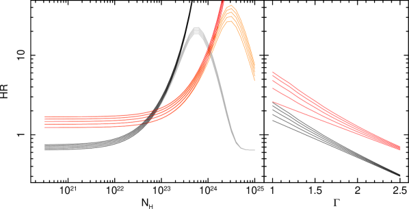
Figure 1: The left-hand panel illustrates the dependence of $HR1\equiv F_{7-10}/F_{2-4}$ (black) and $HR2\equiv F_{10-18}/F_{4-7}$ (red) on $N_{\rm H}$, the total column of gas obscuring an X-ray spectrum with $\Gamma$=1.8 and an Fe K$\alpha$ emission line with an equivalent width of 100 eV. The orange and gray lines respectively denote HR1 and HR2 when there exists an additional power-law component, with $\Gamma=1.8$ and normalization set to 0.01 times that of the primary power law, and absorbed only by $N_{\rm H,Gal}$ = $3\times 10^{20}$ cm^-2. The right-hand panel illustrates the dependence of $HR1$ and $HR2$ on $\Gamma$ when fitting only a simple power law. In both panels, a Compton reflection component modeled with pexrav is included in all cases; the five sets of lines denote spectra with $R$=0.0, 0.5, 1.0, 1.5 and 2.0. Assuming no absorption other than $N_{\rm H,Gal}$ and assuming $R\leq 2.0$, values of $HR1$ greater than $\sim 2$ are only attainable when $\Gamma\la 1.2$.

Hardness ratios alone cannot confirm an increase in absorption. Time-resolved spectra, in many cases, also lack the statistics to rule out such scenarios, and as discussed below, we sometimes must freeze $\Gamma$ to avoid degeneracy between $\Gamma$ and $N_{\rm H}$. For the purposes of identifying candidate eclipse events, we adhere to the assumption that $\Gamma$ intrinsically does not vary to values below 1.4–1.5, and so values of $\Gamma_{\rm app}$ below roughly 1.3 and consequently values of $HR1$ above 1.7 are very likely only due to the presence of significant line-of-sight absorption. We assume that the strength of the Compton reflection hump relative to the power law, also a source of spectral hardening, remains constant over time. For sources that are perpetually X-ray obscured (e.g., the Compton-thin type IIs), we rely on the deviations of $HR1$, $HR2$, and $\Gamma_{\rm app}$ from their mean values to identify potential eclipse events.

Our criteria for a “candidate” eclipse event are thus as follows:

$\bullet$ Criterion 1: trends in $HR1$ (and/or $HR2$ depending on $\Delta$$N_{\rm H}$) that indicate a statistically significant deviation compared to the average spectral state, with a minimum of 2$\sigma$ (standard deviations), and at least a 50 per cent increase above the mean value of $HR1$.

$\bullet$ Criterion 2: at least two consecutive points in a row in the hardness ratio light curve have elevated values. This removes single-point outliers due to statistical fluctuations.

$\bullet$ Criterion 3: trends in $\Gamma_{\rm app}$ that deviate at the $\geq$2$\sigma$ level. ($\Gamma_{\rm app}$ tends to be more statistically noisy than $HR1$, and in most of our candidate events, the deviation in $HR1$ is commonly 1–2$\sigma$ more than the corresponding deviation in $\Gamma_{\rm app}$. Consequently, $HR1$ is our primary selector.) For X-ray unobscured sources, $\Gamma_{\rm app}$ must be lower than 1.3.

To classify an eclipse candidate as “secure,” we impose a fourth criterion:

$\bullet$ Criterion 4: the increase in $N_{\rm H}$ must be confirmed via follow-up time-resolved X-ray spectroscopy in binned spectra.

“Secure” events are divided into “secure A” events, wherein $N_{\rm H}$ and $\Gamma$ are deconvolved in the time-resolved spectra, or “secure B” events, wherein $N_{\rm H}$ has to be determined with an assumed frozen value of $\Gamma$. We define “candidate” events as those satisfying criteria 1–3, but not 4. Such events can be attributed to low signal-to-noise ratio, in terms of either low continuum fluxes or due to the inferred weakness of the event, e.g., values of $N_{\rm H}$ only barely above $1\times 10^{22}$ cm^-2. Qualitatively speaking, the candidate events had large uncertainties on $N_{\rm H}$ even when $\Gamma$ is frozen (e.g., errors spanning factors of more than a few) and/or had large uncertainties on $\Gamma$ (e.g., several tenths or more) when modeling no excess absorption.

3 OVERVIEW OF ECLIPSE RESULTS

We defer all details on individual objects to Appendix A. There, we provide long-term light curves for sub-band continuum fluxes, hardness ratios $HR1$ and $HR2$, and $\Gamma_{\rm app}$. For brevity, we include light curve plots only for the 10 objects with candidate or secure eclipse events; in the other 45 objects, we find no significant sustained deviations in $HR1$, $HR2$ or $\Gamma_{\rm app}$ at the 2$\sigma$ level or greater. However, we also include plots of selected type II objects with evidence for constant, non-zero absorption. Appendix A contains all the details on the observed deviations in the $HR1$, $HR2$, and/or $\Gamma_{\rm app}$ light curves and the subsequent time-resolved spectroscopy. The reader is referred to Lamer et al. (2003), Rivers et al. (2011a), and Akylas et al. (2002) for NGC 3227/2000–1, Cen A, and Mkn 348, respectively; we present new results of time-resolved spectroscopy for all other events.

In this paper, we confirm a total of 12 “secure (A+B)” X-ray absorption eclipses in eight objects (confirmed with spectral fitting) plus four “candidate” eclipses in three objects, all summarized in Table 3. For our 16 secure/candidate events, each with $N_{\rm H}\sim 10^{22-23}$ cm^-2 (see below), each object is bright enough for us to use the 10–18 keV band to probe the uneclipsed continuum. In Appendix A10, we present flux-flux plots that demonstrate that the 2–4 keV flux is affected independently of the behavior of the 10–18 keV continuum during our secure events and that one can distinguish the spectral variability from a discrete eclipse event from that due to variability in the power law. For candidate events, though, the flux-flux plots are unable to fully separate the two types of spectral variability, and this is tied to ambiguity in modeling the time-resolved spectra. Six of these 12 are complete absorption events, with RXTE witnessing both ingress and egress. The events span a range of quality, depending on source brightness, the sampling of the observations, the duration, and $N_{\rm H}$: four events’ column density profiles are well-resolved in time even after binning the observations for time-resolved spectroscopy, allowing constraints on the density profile: Cen A/2010–1, Mkn 348/1996–7, NGC 3227/2000–1, and NGC 3783/2008.3. In contrast, other, more rapid events subtend only two points in the $HR1$ light curve, with only one binned energy spectrum demonstrating increased absorption. Inferred durations range from $<$1 d to a few years, with six secure events’ durations in the $\sim$tens of days range, and three of them $\geq$5 months.

We are sensitive to nearly full-covering absorption by columns in a range of $\sim 10^{22-25}$ cm^-2, but the detected absorption events span only peak column densities of $\sim 4-26\times 10^{22}$ cm^-2, i.e., we see no evidence from our sample for full-covering absorption by Compton-thick clouds. This is not to say that full-covering Compton-thick eclipse events do not occur in Seyferts in general. In other words, although our survey is sensitive to such events, we do not detect any for our monitored sample.

The average values of $N_{\rm H}$ in log space for the two classes (considering only secure events) are nearly identical: 12 and 10 $\times 10^{22}$ cm^-2. In the cases where the column density profiles can be well accessed by several data points after binning for time-resolved spectroscopy, we see no strong evidence for non-symmetric events (along the direction of motion across the line of sight) such as the “comet” shaped clouds inferred by Maiolino et al. (2010) in NGC 1365. The $N_{\rm H}$($t$) and $HR1$($t$) profiles of NGC 3783/2008.3, however, are particularly intriguing: they suggest two peaks separated by $\sim$11 d, but with the values in between the peaks not returning to post/pre-eclipse levels. The possibility of a double-cloud absorption event is discussed further in $\S$5.3. In Table 3, we list parameters both for the full duration and for each clump separately.

Surprisingly, only three type II objects show cloud events. That is, based on their $HR$ light curves, the majority of all other monitored type IIs display no strong evidence (sustained trends in $HR$ more than $50$ per cent above the mean value) for variations in $N_{\rm H}$, although several were individually monitored for several years or more in some cases. In $\S$5.6, we will focus on the nine type II objects that have sustained monitoring for $\geq$0.6 yr. We will show that seven of them lack long-term ($>$1 d) variations in $N_{\rm H}$ down to $\Delta$$N_{\rm H}\sim 1-9\times 10^{22}$ cm^-2 depending on the signal-to-noise ratio and discuss the applicability of clumpy-absorber models to these objects.

In the case of Cen A, in addition to the two eclipses identified, we present in Appendix A evidence (at $\sim$2.2$\sigma$ confidence) that the baseline level of $N_{\rm H}$ dipped by $\sim 14$ per cent and then recovered during the first three months of 2010. The reader should bear in mind, however, that Cen A is a radio galaxy and no BLR has been detected, so it may not be representative of all Seyferts, most of which are radio quiet. This observation and its implications are discussed in $\S$5.6.1.

We caution that “peak $N_{\rm H}$”refers only to what we have measured with time-resolved spectroscopy. Since clouds are not point sources, we can only probe that two-dimensional slice of the cloud that transits the line of sight, and there may exist other lines of sight outside that slice which intersect parts of the cloud with higher columns. Consequently, the intrinsic maximum column density of the cloud could be greater than what we measure if RXTE was not monitoring the source when that part of the cloud transited the line of sight.

The durations we measure also refer only to that slice of the cloud intersected by the line of sight. In the case of a spherically-symmetric cloud, observed eclipse durations will be, on average, $\pi/4$=0.79 times the maximum durations that could have been observed. (Consequently, average inferred cloud diameters, estimated in $\S$5.4, may be underestimated by this modest factor.) In the case of spherical clouds with maximum column density at the center and radial density profiles similar to those for Cen A/2010–1 and NGC 3227/2000–1, then the corresponding effect on peak $N_{\rm H}$ will likely be less than $\sim 20$ per cent.

Table 3: Summary of eclipse events

Source				Duration	Peak $N_{\rm H}$
name	Type	Event	Category	(d)	($10^{22}$ cm-2)	Comments
Type I Secure Events
NGC 3783	Sy1	2008.3	Secure B	14.4–15.4	$11.2^{+1.7}_{-1.5}$	$N_{\rm H}$($t$) resolved.
				$\sim$9.2 & $\sim$4.6	$11.2^{+1.7}_{-1.5}$ & $8.6^{+1.5}_{-1.3}$
Mkn 79	Sy1.2	2003.5	Secure B	12.0–39.4	$14.4^{+4.8}_{-4.2}$‡	Ingress only.
		2003.6	Secure B	34.5–37.9	$11.5^{+3.2}_{-2.8}$
		2009.9	Secure B	19.6–40.0	$7.6\pm 2.2$
Mkn 509	Sy1.2	2005.9	Secure B	$26-91$	$8.8\pm 1.7$‡	Ingress only. $N_{\rm H}$($t$) resolved.
MR 2251–178	Sy1.5/QSO	1996	Secure A	3 – 1641	$6.6^{+0.8}_{-1.4}$‡	Egress before Jun. 1998
NGC 3227	Sy1.5	2000–1	Secure A	77–94	19–26	$N_{\rm H}$($t$) resolved.
		2002.8	Secure B	2.1–6.6	$13.3^{+2.6}_{-2.2}$
Type II Secure Events
Cen A	NLRG/Sy2	$\sim$2003–4	Secure A	$356-2036$	8$\pm$1‡
		2010–1	Secure A	$170.2-184.5$	8$\pm$1	$N_{\rm H}$($t$) resolved.
NGC 5506	Sy1.9	2000.2	Secure A	0.20–0.80	$4.0\pm 1.4$
Mkn 348	Sy2	1996–7	Secure A	$399-693$	$18\pm 3$‡	Egress only. $N_{\rm H}$($t$) resolved.
Candidate Events
Fairall 9	Sy1	2001.3	Candidate	5.4–15.0	$<21$
NGC 3783	Sy1	2008.7	Candidate	17–28	$<4$
		2011.2	Candidate	4.1–15.8	$10.9^{+6.0}_{-5.3}$
NGC 3516	Sy1.5	2011.7	Candidate	$\sim 57$	4.7	Possible variation in covering fraction
						of partial covering, moderately
						highly ionized absorber

Summary of the 12 secure and 4 candidate eclipse events detected. We list events in the order of: secure events in type Is, secure events in type IIs, and then candidate events (which are all for type I objects). “$N_{\rm H}$($t$) resolved” means that at least several consecutive binned spectra confirm increased $N_{\rm H}$ levels. The double-dagger (^‡) indicates that intrinsic peak value of $N_{\rm H}$($t$) may be higher than that observed if it occurred during a gap in monitoring.

4 PROBABILITIES FOR OBSERVING AN X-RAY ECLIPSE EVENT

Ideally, we would like to derive the instantaneous probability $\overline{P_{\rm ecl}}$ of catching a given source while it is undergoing an X-ray eclipse event, and then relate that probability to the source’s optical classification and/or the constant presence/absence of X-ray-absorbing gas along the line of sight. Eclipse events detected in the RXTE archive are, however, evidently rare, with only 10 different objects showing events and with only 1–3 events in each of those objects. We will thus focus in this section on the average instantaneous probability to detect absorption due to an eclipse event for a given class of objects as opposed to individual objects. However, deriving such a probability is not straightforward, because we must factor in biases resulting from our observation sampling, which yields a sensitivity to eclipse durations that is very heterogeneous as a function of timescale, both for object classes and for individual objects. For sustained monitoring, for instance, we are sensitive to a relatively larger number of short-duration eclipses than to long-duration eclipses. For example, given a hypothetical campaign consisting of one observation daily for 64 d, we can detect a maximum of 16 full eclipses of duration 3 d (4 points), 8 full eclipses of duration 7 d (8 points), etc.

We thus quantify an instantaneous probability density $p_{\rm ecl}$ as a function of eclipse duration as follows: we first define for each individual object a “selection function” $SF_{\rm ind}$ to quantify our sensitivity, as a function of eclipse duration, to the maximum total number of eclipses which could have been potentially observed, given that object’s sampling with RXTE; this procedure is described in $\S 4.1$. We then produce summed selection functions $SF_{\rm sumI,II}$ to quantify the average sensitivity to the total number of eclipses for each object class (type I and II), as well as to identify potential biases affecting a given object class as a whole. In $\S 4.2$, we quantify the total number of eclipse events $N_{\rm ecl}$ actually observed within each object class as a function of eclipse duration. Then, in $\S 4.3$, as we have binned our observed events and the selection functions (maximum possible event number) on to the same grid as a function of eclipse duration, we divide $N_{\rm ecl}$ by $SF_{\rm sumI,II}$ to obtain the instantaneous probability density $p_{\rm ecl}$($t_{\rm i}$). This quantifies the likelihood to witness an eclipse as a function of that eclipse’s duration, defined over a discrete set of timescale bins $t_{\rm i}$. Finally, we integrate $p_{\rm ecl}$($t_{\rm i}$) over all timescale bins to obtain $\overline{P_{\rm ecl}}$, the instantaneous probability of witnessing a source in eclipse for any eclipse duration.

As a reminder, $\overline{P_{\rm ecl}}$ and $p_{\rm ecl}$($t_{\rm i}$) do not necessarily denote the likelihood to simply observe a source with non-zero X-ray obscuration; this holds true only if the source normally devoid of X-ray-absorbing gas along the line of sight. $\overline{P_{\rm ecl}}$ and $p_{\rm ecl}$($t_{\rm i}$) refer to the likelihood of catching the source in state with a higher-than-usual value of $N_{\rm H}$ at any instant due specifically to a discrete (localized in time) eclipse event by a cloud of gas, one that transits the line of sight with an observed duration between $t_{\rm i}$ and $t_{\rm i+1}$ in the case of $p_{\rm ecl}$($t_{\rm i}$). In $\S$5.5, we will compare our estimates of $\overline{P_{\rm ecl}}$ for each class to the predictions for a clumpy torus to cause a given source to be observed in eclipse.

4.1 Selection functions

This section describes how we generate “selection functions” for each individual object $SF_{\rm ind}$($t_{\rm i}$) and sum selection functions for each object class $SF_{\rm sumI,II}$($t_{\rm i}$) to quantify the number of light curve observation segments (“campaigns”) of a given duration as a function of event duration. Here we define a “campaign” as consisting of a minimum of four observations, with no single gap between adjacent observations being greater than 75 per cent of the duration.

We define 19 time bins $t_{\rm i}$ spanning from 0.20 to 5850 d, with time bins equally spaced by 0.235 in log space; in linear space, the $i$th time bin is defined by $0.20\times$($1.718^{i}$) d $\leq t<0.20\times$($1.718^{i+1}$) d, with $i=0...18$. $SF_{\rm ind}$($t_{\rm i}$) effectively tells us the potential maximum number of eclipse events of duration $t_{\rm D}$ satisfying $t_{\rm i}\leq t_{\rm D}<t_{\rm i+1}$ that RXTE was capable of potentially catching, given the observed sampling for that object.

The $SF_{\rm ind}$($t_{\rm i}$) are constructed as follows: consider a light curve with $J$ total observations (data points), and observation times denoted by $X_{j=1}$ … $X_{j=J}$. For each time bin $t_{\rm i}$, we start at $j=1$ and we identify the first light curve segment $X_{1}..X_{q}$ whose duration $t_{\rm D}$ satisfies $t_{\rm i}\leq t_{\rm D}<t_{\rm i+1}$. We require a minimum of four data points, since we defined above an eclipse event relying on a minimum of two consecutive points to form a significant peak in the $HR$ light curves, plus one point before and one point after the putative eclipse to denote the “baseline” levels of $HR$. The goal is to have consistency between detecting real eclipse events and how we determine the maximum possible number of potential eclipse events. Consequently, we disqualify a segment if any gap between two adjacent points is $>75$ per cent of the segment’s duration. If the segment $X_{1}...X_{q}$ satisfies these criteria, then $SF_{\rm ind}$($t_{\rm i}$) = $SF_{\rm ind}$($t_{\rm i}$) +1, and we restart counting from point $X_{q+1}$. Otherwise, we restart from $j=2$.

When there existed sustained monitoring with a sampling interval $\Delta$$t$ for a duration $t_{\rm D}$, we are sensitive to eclipse events on a continuous range of timescales from $4\Delta$$t$ up to $t_{\rm D}$, with $SF_{\rm ind}$($t_{\rm i}$) increasing towards shorter timescales. RXTE monitored 42 sources continuously for $\sim$1 yr and longer (sun-angle gaps notwithstanding), and one of the most common sampling times for these programmes was 3–4 d. Many objects’ selection functions thus feature peaks in the 8.8–15.2 d time bin, with a sharp drop-off in $SF_{\rm ind}$($t_{\rm i}$) below 8.8 d. In addition, there were multiple intensive-monitoring programmes featuring observations several times daily for durations of days to weeks. These programmes lead to large contributions in $SF_{\rm ind}$($t_{\rm i}$) from $\sim$1 to several days. As an example, we consider the case of Mkn 79, which had monitoring observations every $\sim$10 d for a duration of 309 d (MJD 51610–51919), every $\sim$2 d for 15.6 d (MJD 51754.5–51770.1), every $\sim$2 d for 3205 d (MJD 52720–55925) with $\sim$26 d gaps once a year due to sun-angle constraints, and every $\sim 6$ hr for 64.6 d (MJD 53691.4–53756.0). The $F_{2-10}$ light curve and the corresponding selection function are plotted in Figs. 2 and 3, respectively.

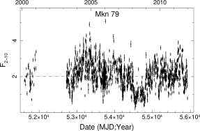
Figure 2: 2–10 keV observed light curve for Mkn 79. This plot only shows the general trend of the hard flux and does not serve to identify any candidate eclipse events.

Figure 3: Selection function $SF_{\rm ind}$($t_{\rm i}$) for Mkn 79. The histogram quantifies the number of “campaigns” per timescale bin and is computed on the base of the light curve in Fig. 2.

We create summed selection functions for each object class as a function of timescale bin ($SF_{\rm sumI,II}$($t_{\rm i}$)) by summing up the individual selection functions for the 37 type I and 18 type II AGN separately (left- and right-hand panels of Fig. 4). We see that the number of campaigns per given timescale is on average 3.9 times greater for the type Is than for the type IIs. For both classes, the most common campaign timescales are $\sim$tens of days.

Due to the heterogeneous sampling in the archive, some objects can contribute as many as 200–300 campaigns to an individual $t_{\rm i}$ bin (usually the 8.8–15.2 d bin) while other objects were observed much more sparsely and yield selection functions containing only a few campaigns to a few timescale bins. To estimate the uncertainty on each binned $SF_{\rm sumI,II}$($t_{\rm i}$) point stemming from the varying contributions of individual source selection functions, we employ a Monte Carlo bootstrap procedure. For each object class (type I or type II) of $N_{\rm S}$ objects, we do the following $m=1000$ times: we select at random one individual selection function from the pool of observed $SF_{\rm ind}$ functions, until a total of $N_{\rm S}$ individual selection functions was accumulated. We explicitly allow for individual objects to be selected multiple times. We sum those to create a simulated summed selection function $SF^{i}_{\rm sum}$, where $i\in{1...m}$. Once we have $m$ $SF^{i}_{\rm sum}$ functions, we calculate the standard deviation within each bin to yield the relative uncertainties plotted in Fig. 4. This procedure yields typical bin uncertainties of $\sim$12 and 25 per cent for type Is and IIs, respectively.

Figure 4: Summed selection functions $SF_{\rm sumI}$($t_{\rm i}$) and $SF_{\rm sumII}$($t_{\rm i}$) for the 37 type I and 18 type II AGN, respectively. These figures illustrate the total number of observation “campaigns” (maximum number of potential detected eclipses) per timescale bin $t_{\rm i}$. The 1$\sigma$ uncertainties are determined by a Monte Carlo bootstrap method.

Figure 5: Number of different objects that contribute to a given timescale bin for type I (left) and type II (right) AGN.

We also plot for each object class the number of different objects that contribute to a given timescale bin (Fig. 5). These plots can identify those timescales over which biases arise because only a small number of different objects contribute to the relevant eclipse duration bin. For both classes of objects, the number of objects contributing to a given timescale is roughly constant from $\sim$1 to $\sim$300 d, but drops off rapidly above $\sim$300 d in the type IIs. In fact, for the type IIs, timescales above 400 d are probed by only 3–5 objects. Especially in the case of type IIs, we are thus relying on the assumption that these few objects (Cen A, NGC 1052, NGC 4258, NGC 5506, and NGC 7314) are truly representative of the whole class in terms of their variable X-ray absorption properties, since they strongly influence our inferences about variable absorption in type IIs on these long timescales.

4.2 Number of observed events per timescale bin

In Fig. 6, we plot the number of eclipse events as a function of each of their durations, using the same 19 timescale bins as above. In the upper panel for each class, each eclipse event is depicted by a separate symbol/bar. In these panels we plot all eclipse events independent of the data quality of the eclipse (13 secure A+B and 3 candidate events). In the lower panel for each class we plot histograms denoting the number of observed eclipses as a function of timescale bin $N_{\rm ecl}$($t_{\rm i}$). The black solid line is the “best estimate” of $N_{\rm ecl}$($t_{\rm i}$), using only the best-estimate values of the durations and ignoring the candidate events.

We also present estimates of $N_{\rm ecl}$($t_{\rm i}$) that correspond to the maximum and minimum likelihoods of witnessing sources in eclipse, given that an event’s contributions to $N_{\rm ecl}$($t_{\rm i}$) may shift in $t_{\rm i}$ given the measured uncertainties in the observed duration. For each eclipse event, we thus considered those timescale bins $t_{\rm i}$ consistent with the limits of the observed duration (as identified in Fig. 6), and identified which one of those timescale bins $t_{\rm i}$ had the highest corresponding value of $SF^{i}_{\rm sumI,II}$ (lowest probability associated with one single eclipse event). The orange line denotes the final $N_{\rm ecl}$($t_{\rm i}$) histogram corresponding to the minimum probability densities, accumulated over all secure events within each class. The green solid line in each lower panel, meanwhile, denotes $N_{\rm ecl}$($t_{\rm i}$) corresponding to the highest probability densities, computed in a similar fashion as the orange solid line, but this time including the candidate events as well.

For type I AGN, the ”typical” observed duration timescale is tens of days, although this may not be surprising given the strong peak of the selection function at tens of days. The case of MR 2251–178 is very exceptional, as we detect clear signs for a secure eclipse event but have only poor constraints on its duration ($3$ d $<t<$ 4.5 yr). If we ignore this event, we do not have any type I eclipses that are consistent with an event duration longer than 100 d despite the numerous campaigns lasting for several hundreds of days to several years. Even though the shapes of the selection functions for type I and IIs are extremely similar, for type II objects, we do not detect any eclipse events with durations in the range 1–100 d. The three type II eclipses with durations of $>$100 d have more than five times fewer observing campaigns than between 10 and 30 d where the maximum of the summed selection function for type II objects occurs. In other words, the histogram of type I eclipses agrees well with the expected distribution based on the summed selection function of type I objects, while type II eclipses do not appear at the expected duration if only their summed selection function is considered.

Figure 6: Number of observed eclipse events $N_{\rm ecl}$ as a function of timescale bin $t_{\rm i}$ for the type I AGN (top pair of panels) and type II (bottom pair). Within each object class, we plot the observed durations for each eclipse in the top of each pair. In the case of MR 2251–178, the star denotes the average of the minimum/maximum eclipse durations in log space, as constraints for the best estimate of the actual duration are poor. Candidate eclipses are shown in gray. In each lower panel, the black line indicates the “best estimate” of $N_{\rm ecl}$($t_{\rm i}$), using only the best-estimate values of the durations and excluding candidate eclipses. The orange line is the minimum of $N_{\rm ecl}$($t_{\rm i}$) (i.e., the minimum possible number of events with duration $t_{\rm i}\leq D<t_{\rm i+1}$). The green line is the maximum of $N_{\rm ecl}$($t_{\rm i}$) (i.e., the maximum possible number of events with duration $t_{\rm i}\leq D<t_{\rm i+1}$), including candidate eclipses.

4.3 Calculating the instantaneous eclipse probability densities $p_{\rm ecl}$($t_{\rm i}$) and the instantaneous eclipse probability $\overline{P_{\rm ecl}}$

Given the values of $N_{\rm ecl}$($t_{\rm i}$) corresponding to the best estimates of duration, we can now estimate the corresponding function of $p_{\rm ecl}$($t_{\rm i}$) for each class by dividing each bin of $N_{\rm ecl}$($t_{\rm i}$) by $SF_{\rm sumI,II}$($t_{\rm i}$). The resulting function of $p_{\rm ecl}$($t_{\rm i}$) for each class is plotted as the black solid lines in Fig. 7. As a reminder, $p_{\rm ecl}$($t_{\rm i}$) describes the likelihood to catch a source undergoing an eclipse due to one specific kind of cloud: one that results in an eclipse with a duration $t_{\rm i}\leq D<t_{\rm i+1}$. The errors on individual points of $p_{\rm ecl}$($t_{\rm i}$) take into account the error in the selection function obtained from the bootstrapping method only.

The minimum- and maximum-likelihood $p_{\rm ecl}$($t_{\rm i}$) functions are calculated in a similar way, although we divide by $SF_{\rm sumI,II}$($t_{\rm i}$) $\pm$ $\sigma_{\rm SF}$($t_{\rm i}$), where $\sigma_{\rm SF}$($t_{\rm i}$) denotes the uncertainties in $SF_{\rm sumI,II}$($t_{\rm i}$) as determined by the Monte Carlo bootstrap method; the minimum and maximum functions are, respectively, the orange and green solid lines in Fig. 7. Because $p_{\rm ecl}$($t_{\rm i}$) is in log space, any bin with zero probability density is plotted as $10^{-6}$. “Typical” values of $p_{\rm ecl}$($t_{\rm i}$) when eclipses are detected are $\sim 10^{-(2.8-3.4)}$ for type Is and $\sim 10^{-(1.3-2.2)}$ for type IIs. We must caution the reader that most probability density values are on the order of 1/$SF_{\rm sum}$($t_{\rm i}$). We display 1/$SF_{\rm sum}$($t_{\rm i}$) in Fig. 7 via cyan and magenta lines for types I and II, respectively. Consequently, the detection of one eclipse within these duration bins would strongly influence the inferred $p_{\rm ecl}$($t_{\rm i}$) profile. Nonetheless, the data suggest that eclipses of any duration generally occur more frequently in type IIs.

In type IIs, we do not detect events of durations $\sim$tens of days, for which one event for a given timescale bin would have yielded a probability density of $\sim$ 1/200 – 1/1000. If it were the case that eclipses with durations of $\sim$tens of days occurred in type IIs with the same probability density as in type Is, $\sim 10^{-(2.8-3.4)}$, our observations would likely not have detected them. This is because the values of those $p_{\rm ecl}$($t_{\rm i}$) points would lie below the detection threshold for eclipses in type IIs, represented by 1/$SF_{\rm sumII}$($t_{\rm i}$), the magenta line in the lower panel of Fig. 7; recall that there were $\sim$3-4 times fewer campaigns for type IIs as there were for type Is.

In type Is, we did not detect events of durations $\sim$hundreds of days (although such a duration cannot be ruled out in the case of MR 2251–178), for which one event for a given timescale bin would have yielded a probability of $\sim$ 1/200 – 1/1000. If it were the case that eclipses with durations of $\sim$hundreds of days occurred in type Is with the same probability density as in type IIs, then the number of monitoring campaigns for type Is would have clearly allowed us to detect them. If this were the case, then the resulting $p_{\rm ecl}$($t_{\rm i}$) values for type Is would appear in the upper panel of Fig. 7 with values higher than the detection threshold, represented by 1/$SF_{\rm sumI}$($t_{\rm i}$), the cyan lines.

Finally, we sum up the values of $p_{\rm ecl}$($t_{\rm i}$) over all timescale bins to obtain estimates of $\overline{P_{\rm ecl}}$. More specifically, best-estimate, minimum and maximum values of $\overline{P_{\rm ecl}}$ can be obtained by summing the functions of $p_{\rm ecl}$($t_{\rm i}$) denoted by the black, orange, and green histogram lines, respectively, in Fig. 7. However, we must bear in mind that we have a very small number of total events, and many timescale bins contain only $\sim 0-1$ events. When summing to obtain the maximum value of $\overline{P_{\rm ecl}}$, we opt to be conservative and take into account the selection function, the reciprocal of which denotes the likelihood of witnessing just one event with duration $t_{\rm D}$ satisfying $t_{\rm i}\leq D<t_{\rm i+1}$. For each $t_{\rm i}$, we use the maximum of either $1/SF_{\rm sumI,II}$($t_{\rm i}$) (cyan/magenta lines in Fig. 7) or $p_{\rm ecl}$($t_{\rm i}$) (green line). To reiterate, our uncertainties on $\overline{P_{\rm ecl}}$ are conservative estimates in that they take into account the effect of uncertainties in duration on $N_{\rm ecl}$($t_{\rm i}$), the uncertainties in $SF_{\rm sumI,II}$($t_{\rm i}$) as determined by the Monte Carlo bootstrap method, the effects of the selection function, and the presence of candidate events on the maximum probability. Our final estimate for $\overline{P_{\rm ecl}}$ for type Is is 0.006 with a range of 0.003–0.166 (minimum – maximum probability). For type IIs, $\overline{P_{\rm ecl}}$=0.110, with a range of 0.039–0.571. That is, based on our best estimates, type II AGN have a $\sim 18$ times higher chance of showing an eclipse (of any duration). These values are summarized in Table 4, and we return to these values later in $\S$5.

We caution that these probabilities refer only to eclipses by full-covering, neutral or lowly-ionized clouds with columns densities $\ga 10^{22}$ up to $\sim 10^{25}$ cm^-2; when one considers the full range of clouds (larger range of $N_{\rm H}$, partial-covering clouds, wider range of ionization) the resulting probabilities will almost certainly be higher.

Table 4: Inferred probabilities $\overline{P_{\rm ecl}}$ to witness a source undergoing an eclipse event

Object	$\overline{P_{\rm ecl}}$	$\overline{P_{\rm ecl}}$	Limits on
class	(Best	(Min.–max.	$\overline{P_{\rm ecl}}$ for Compton-
	estimate)	range)	thick events
Type Is	0.006	0.003–0.166	$<0.158$
Type IIs	0.110	0.039–0.571	$<0.520$

Ramos Almeida et al. (2011) noted that the IR SEDs of Sy 1.8–1.9 AGN had spectral slopes intermediate between those of Sy 1.0–1.5s and Sy 2s, and noted similarities in SED fitting parameter results between the 1.8–1.9s and the 1.0–1.5s. However, we simply do not have enough events to break up the probability estimates for type IIs into further subclasses, and cannot address this point. If we break up the type Is into Sy 1.0s/1.2/1.5s, tantalizingly, the best-estimate values for $\overline{P_{\rm ecl}}$ increase with subclass: 0.0003, 0.0024, and 0.0036, consistent with the notion that relatively higher levels of obscuration exist in higher numbered subclasses. However, the (conservatively-determined) minimum and maximum values indicate nearly identical ranges ([0.0003-0.1586], [0.0014-0.1597], and [0.0013-0.1619]) because with only $\sim 0-1$ events per timescale bin, the maximum values tended towards the integral of $1/SF_{\rm sum1.0/1.2/1.5}$($t_{\rm i}$). Furthermore, any conclusions would be based on a mere 1–4 secure eclipse events and 1–3 objects per subclass, and so we do not address the subclasses further.

In $\S$3, we noted that we did not detect any Compton-thick obscuration events, but this is not to say with full certainty that such events cannot exist. A conservative upper limit on the probability to observe a Compton-thick event of any duration between 0.2 d and 16 yr is obtained by summing $1/SF_{\rm sumI,II}$($t_{\rm i}$): $\overline{P_{\rm ecl}}<0.158$ (type Is) or $<0.520$ (type IIs).

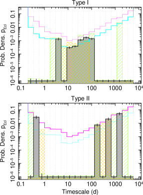
Figure 7: The probability density functions $p_{\rm ecl}$($t_{\rm i}$) for each class denote the instantaneous likelihood of witnessing a source undergoing an eclipse event with eclipse duration between $t_{\rm i}$ and $t_{\rm i+1}$. They are calculated by dividing the $N_{\rm ecl}$($t_{\rm i}$) functions in Fig. 6 by the summed selection functions $SF_{\rm sumI,II}$($t_{\rm i}$) in Fig. 4. The black solid line corresponds to the best-estimate durations; the vertical black bars denote the relative uncertainties derived from uncertainties in the summed selection function. The orange and green solid lines denote the functions $p_{\rm ecl}$($t_{\rm i}$) that minimize or maximize, respectively, the likelihood of occurrence given the limits on each observed event duration (see text for details). Because $p_{\rm ecl}$($t_{\rm i}$) is in log space, zero probabilities are plotted as $10^{-6}$ for clarity. The cyan and magenta lines denote 1/$SF_{\rm sumI}$($t_{\rm i}$) and 1/$SF_{\rm sumII}$($t_{\rm i}$), respectively. The thin magenta line in the top panel and the thin cyan line in the lower panel denote 1/$SF$ of the other object class to allow visual comparison between both object classes.

5 DISCUSSION

There has been much work so far into variable X-ray absorption in AGN. The accumulated research so far, including this work, has revealed eclipse events spanning a wide range of observed durations, ionization levels, and including full or partial covering.

Most of the short-term events (durations $\la 1-3$ d) have been observed in the prominent case of the Sy 1.8 NGC 1365, where rapid and strong variations in $N_{\rm H}$ are observed in a very large fraction of observations. The clouds are inferred to exist in the BLR and are frequently modeled via variations in covering fraction of partial-covering material (e.g., De Rosa et al. 2007; Turner et al. 2008; Risaliti et al. 2011). In the context of clumpy-absorber models, there can exist a variable number of clouds in the line of sight at any given time, with a relatively extended X-ray continuum source located behind them.

RXTE, in contrast, has detected full-covering, cold or at most modestly ionized clouds. An emerging picture is that clouds in the BLR and clouds in the torus may be two manifestations of the same radially extended cloud distribution, existing inside and outside, respectively, the dust sublimation region (Elitzur 2007). That is, in the simplest picture, the full-covering clouds detected with RXTE are part of the same population of clouds as those causing the short-duration events, just occurring at larger radii, as we will demonstrate in $\S$5.2.

It is potentially interesting that 4 of the 10 sources in our sample with secure or candidate eclipse events have multiple such events (certain objects thus seem to be prone to a higher frequency of events than others). The high frequency of events observed in NGC 1365 may potentially be explained by a favorable geometry/viewing angle. However, NGC 1365 may be a special object; a statistical sample on a large number of AGN may be better suited to quantify eclipse events across all AGN.

5.1 Dependence of cloud events on AGN physical parameters

Having identified secure and candidate eclipses in 10 of the 55 objects monitored with RXTE, we can attempt to explore if certain system parameters govern the presence or lack of eclipsing clouds. For example, the 10 sources’ black hole masses (see $\S$5.2) span log($M_{\rm BH}$) = 6.9–8.8, and these values are not extreme compared to black hole masses for Seyferts/quasi-stellar objects (QSOs) in general or our whole sample.

There is no evidence that having an extreme value of luminosity governs the presence/lack of eclipses: the range of log($L_{2-10}$) and log($L_{\rm Bol}$) where eclipses are confirmed with RXTE to occur are 41.93–44.73 and 42.9–45.6, respectively. Again, these values are not extreme.

In the context of clouds being produced in a disk wind, Elitzur & Ho (2009) estimate that such winds cannot exist when the bolometric luminosity drops below $5\times 10^{39}$ ($\frac{M_{\rm BH}}{10^{7}\rm M_{\odot}}$)^2/3 erg s^-1. However, we cannot test this with our sample, as the lowest-luminosity objects monitored with RXTE have 2–10 keV luminosities of $2-6\times 10^{40}$ erg s^-1 (NGC 4258, NGC 3998, and NGC 4051).

Accretion rate relative to Eddington, $L_{\rm Bol}/L_{\rm Edd}$, is also not an obvious factor; values of $\dot{m}$ for the 10 objects span $\sim 0.1$ per cent for Cen A up to $\sim 16$ per cent for MR 2251–178, with most other objects’ values in the range of 3–10 per cent. These values are typical for Seyferts in general as well as for our sample.

Can radio loudness be a factor? One of our eight sources with secure eclipses is radio loud, compared to 13/55 (24 per cent) sources in the original sample. If we start with 55 objects, 13 of which are radio loud, and select at random eight of the 55 for a sub-sample, the probability $P(X=k)$ that exactly $k$ out of eight sources in the subsample will be radio loud is given by the hypergeometric distribution

$$P(X=k)={K\choose k}{N-K\choose n-k}\Big{/}{N\choose n}\ ,$$ (1)

where $N=55$ is the population size, $K=13$ is the number of successes in the population (radio-loud sources), and $n=8$ and $k$ are the sample size and the number of successes in the sample, respectively. ${\cdot\choose\cdot}$ is a binomial coefficient. The chance of having exactly $k=0,1,2,3$ or $4$ radio-loud sources in a random sample of eight is $P(X=0,1,2,3,$ or $4)=$ (0.10, 0.29, 0.34, 0.20, or 0.07). In other words, it is almost as likely to have exactly 1/8 radio-loud sources in the sub-sample as it is to have 2/8 radio-loud sources. There is thus no significant statistical evidence that our sub-sample of sources with secure eclipses is unusual compared to the original sample in terms of fraction of radio-loud sources.

In summary, we find no evidence for a strong dependence of the presence of eclipse events as a function of the most common AGN parameters. One has to keep in mind that only strong correlations could have been detected with our relatively small number of observed events. That being said, the reader is reminded that with a high dynamic range of sampling for 55 objects totaling 230 object-years of monitoring, this study is by far the largest available data set for testing the environment close to supermassive black holes via eclipse events over timescales longer than a few days.

5.2 Locations of X-ray obscuring clouds

Constraints on the distance from the X-ray continuum source to each cloud $r_{\rm cl}$ can be derived from the cloud’s ionization level, column density, and eclipse duration. Following, e.g., $\S$4 of Lamer et al. (2003), we assume for simplicity that each cloud has a uniform density and ionization parameter, and that clouds are in Keplerian orbits. The cloud diameter $D_{\rm cl}$ = $N/n_{\rm H}=v_{\rm cl}t_{\rm D}$, where $t_{\rm D}$ is the cloud’s crossing time across the line of sight and $v_{\rm cl}$ is the transverse velocity, equal to $\sqrt{GM_{\rm BH}/r_{\rm cl}}$. Solving for $r_{\rm cl}$ and using the definition of $\xi$, one obtains (see, e.g., Eqn. 3 of Lamer et al. 2003): $r_{\rm cl}=4\times 10^{16}M_{7}^{1/5}L_{42}^{2/5}t_{\rm D}^{2/5}N_{\rm H,22}^{-2/5}\xi^{-2/5}$ cm, where $M_{7}=M_{\rm BH}/10^{6}\rm M_{\odot}$, $L_{42}=L_{\rm ion}/$($10^{42}$ erg s^-1), $N_{\rm H,22}=N_{\rm H}/$($10^{22}$ cm^-2), and $t_{\rm D}$ is in units of days.

Table 5 lists the inferred values of $r_{\rm cl}$, obtained as follows: we use estimates of $M_{\rm BH}$ from reverberation mapping where available; otherwise, estimates are from stellar kinematics or gas dynamics, based on empirical relations between optical luminosity and optical line widths, or from modeling reprocessing in accretion disks. The references are listed in column 4 of Table 5.

For all objects except Cen A, we estimate $L_{\rm ion}$ as follows: we use the best-fitting unabsorbed power law from Rivers et al. (2013), and extrapolate to the 0.1–13.6 keV range to estimate the luminosity $L_{\rm 0.1-13.6keV}$. The luminosity below $\sim$0.1 keV, however, is expected to contain significant contributions from the thermal accretion disk continuum emission. Vasudevan & Fabian (2009) estimate that the ratio of the 0.0136–0.1 keV luminosity to the bolometric luminosity, $L_{\rm 0.0136-0.1keV}/L_{\rm Bol}$, ranges from 0.2 to 0.6 for values of $L_{\rm Bol}/L_{\rm Edd}$ ranging from 0.01 to 0.6, respectively. We take values of $L_{\rm Bol}$ and $L_{\rm Bol}/L_{\rm Edd}$ from Vasudevan et al. (2010) when available. However, for Fairall 9 the value of $L_{\rm Bol}$ is taken from Vasudevan & Fabian (2009), and for MR 2251–178, we use the 2–10 keV flux from Rivers et al. (2013) and we estimate $L_{\rm Bol}/L_{\rm Edd}=40$ from Marconi et al. (2004). We then assume for simplicity a linear dependence of log10($L_{\rm 0.0136-0.1keV}/L_{\rm Bol}$) on log10($L_{\rm Bol}/L_{\rm Edd}$) to estimate $L_{\rm 0.0136-0.1keV}$, and add that to $L_{\rm 0.1-13.6keV}$ to obtain the values of $L_{\rm ion}$ listed in Table 5. The broadband SED of Cen A is more like that of blazars than radio-quiet Seyferts, with a broad inverse-Compton hump dominating the emission from the optical band to gamma-rays. We assume $\Gamma=1.84$ (Rivers et al. 2013) over 0.4–13.6 keV, breaking to $\Gamma=1.0$ over 0.0136–0.4 keV (Steinle 2010; Roustazadeh & Böttcher 2011); this yields $L_{\rm ion}$ = $10^{42.3}$ erg s^-1.

Our constraints on the ionization parameters for our clouds are poor. Given the column densities of our clouds and the energy resolution of the PCA, we can safely rule out values of log($\xi$) above $\sim 2$. In that case, the absorber would manifest itself above 2 keV only via discrete lines and edges, as opposed to a broad rollover towards lower energies. We therefore calculate distances assuming log($\xi$) = –1, 0, or +1. Uncertainty on $r_{\rm cl}$ is thus dominated by uncertainty on $\xi$. For brevity, we list in Table 5 only values assuming log($\xi$)=0. Because $r_{\rm cl}\propto\xi^{-2/5}$, values of $r_{\rm cl}$ assuming e.g., log($\xi$) = –1 or +1 are only factors of 2.5 larger or smaller, respectively. However, for Cen A, we do not consider log($\xi$) = +1. We fit the spectrum of the most absorbed spectral bin used in Rivers et al. (2011b), model the absorption with an xstar table, and obtain log($\xi$) $\la-0.1$. Similarly, for NGC 3227/2000–1, Lamer et al. (2003) found log($\xi$) = –0.3–0 from a contemporaneous XMM-Newton observation. These two events have among the highest quality energy spectra in the group, and one might speculate that such an ionization level may be representative of the rest of the sample. For the candidate event in NGC 3516, we use the best-fitting ionization from Turner et al. (2008), log($\xi$)=2.19, as explained in Appendix A. Finally, we note that although for a few events, it is difficult to estimate reliable uncertainties on $t_{\rm d}$, a $\pm 10$ per cent uncertainty on $t_{\rm d}$ translates into only $\pm 4$ per cent uncertainty in $r_{\rm cl}$.

We obtain best-estimate values of $r_{\rm cl}$ that are typically tens to hundreds of light-days from the central engine, and lie in the range $1-50\times 10^{4}R_{\rm g}$ ($0.3-140\times 10^{4}R_{\rm g}$ accounting for uncertainties), where $R_{\rm g}\equiv GM_{\rm BH}c^{-1}$. We now compare these inferred radii to the locations of typical emitting components in AGN. In Table 16 we list inferred locations for the origins of optical and near-IR broad emission lines and “hidden” broad lines observed in polarized emission for type IIs, locations of IR-emitting dust determined via either interband correlations or IR interferometry, and locations of Fe K$\alpha$ line-emitting gas determined via either X-ray spectroscopy or variability. For reverberation mapping of emission lines, we use time-lag results when available, otherwise we use full width at half-maximum (FWHM) velocities $v_{\rm FWHM}$, assumed for simplicity Keplerian motion, and estimate radial locations via $r=GM_{\rm BH}/(\frac{3}{4}v_{\rm FWHM}^{2})$.

The results are also plotted in Fig. 8 in units of $R_{\rm g}$ for each object. All structures for a given object in Fig. 8 are plotted on one dimension for clarity, but they do not necessarily overlap in space (e.g., X-ray clouds must lie along the line of sight, but other structures may lie out of it). The objects are listed in order of increasing $R_{\rm d}$/$R_{\rm g}$. The black points denote the estimates for $r_{\rm cl}$ assuming log($\xi$)=0, but we denote the minimum/maximum range assuming log($\xi$)= –1 to +1 by the gray areas (again, with –1 to 0 for Cen A and –0.3 to 0 for NGC 3227/2000–1).

The radial distance from the black hole where dust sublimates can be estimated via $R_{\rm d}\sim 0.4(L_{\rm bol}/10^{45}{\rm ergs}^{-1})^{1/2}(T_{\rm d}/T_{\rm 1500})^{-2.6}~{}{\rm pc}$, where $T_{\rm d}$ is the dust sublimation radius, here assumed to be 1500 K (Eqn. 2.1 of Nenkova et al. 2008b). However, the boundary between dusty and dust-free zones is likely highly blurred, because relatively larger grains can survive at higher temperatures. In addition, individual components of dust can sublimate at different radii, e.g, graphite grains sublimate at a slightly higher temperature than silicate grains (Schartmann et al. 2005). We use the above equation as an approximation for the outer boundary of the ”dust sublimation zone” (DSZ), i.e., we assume that no dust sublimation occurs outside $R_{\rm d}$. We take the inner boundary of the DSZ to be a factor of $\sim$2–3 smaller than $R_{\rm d}$. For example, Nenkova et al. (2008b) point out that the $V$–$K$ band reverberation lags measured by Minezaki et al. (2004) and Suganuma et al. (2006) are $\sim 2-3$ times shorter than the light travel times predicted by the above equation. Those experiments thus may be tracking the innermost, larger grains. For simplicity, we assume that the central engine emits isotropically. The estimated values of $R_{\rm d}$ are listed in Table B1, with dusty regions represented by the purple areas in Fig. 8, and the inferred DSZs represented by the fading purple areas.

We list the radial locations of each cloud in units of $R_{\rm d}$ in Table 5. The clouds in 7/8 objects are consistent with residing in the DSZ considering uncertainties on $r_{\rm cl}$. However, this “clustering” may be in part associated with our observational bias to select eclipses with events of $\sim$tens of days, as per our selection function. In Cen A, the clouds are inferred to be consistent with residing entirely in the dusty zone. In contrast, NGC 5506 has the lowest value of $r_{\rm cl}$/$R_{\rm d}$; those clouds are likely the least dusty of the secure events in our sample.

The IR-emitting structures for Cen A, NGC 3783, and NGC 3227 as mapped by either interferometric observations or optical-to-near-IR reverberation mapping are inferred to exist at radii $r_{\rm IR}\sim 3-20\times 10^{4}R_{\rm g}$. Although we can only make a statement based on three objects, values of $r_{\rm cl}$ are generally consistent with these structures, again supporting the notion that the X-ray-absorbing clouds detected with RXTE are thus likely dusty.

For six of the seven objects with known BLRs (MR 2251–178, Mkn 509, Mkn 79, NGC 3783, NGC 3227, and Mkn 348), the BLR clouds are inferred to exist at $r_{\rm BLR}\sim 0.1-2\times 10^{4}R_{\rm g}$ from the black hole. We thus discuss our results in the context of the notion put forth by Netzer & Laor (1993) that the outer radius of the BLR may correspond to $R_{\rm d}$ and the inner radius of the dusty torus, supported by the results of Suganuma et al. (2006). In these six objects, one can see from Fig. 8 that the radial ranges of $r_{\rm BLR}$ are generally smaller than those for both $r_{\rm cl}$ and $r_{\rm IR}$. That is, best-estimate values of $r_{\rm cl}$ are generally commensurate with the outer portions of the BLR or exist at radii up to $\sim$15 times that of the outer boundary of the BLR, although we must caution that we are dealing with a very small sample of only six objects.

We can conclude that, at least for these six objects, the X-ray-absorbing clouds are likely more consistent with the dusty torus than with the BLR. Note that this conclusion is relatively robust to our assumed values of log($\xi$); even if log($\xi$)=+2, the X-ray-absorbing clouds would be closer to the black hole by only a factor of 2.5. Our results thus demonstrate that radii commensurate with the outer BLR and with the inner dusty torus are radii where X-ray-absorbing clouds may exist.

The seventh object with measured BLR parameters is NGC 5506, where $r_{\rm BLR}\sim 4-10\times 10^{4}R_{\rm g}$ based on IR emission lines. The inferred radial location of the X-ray cloud is $0.3-4.5\times 10^{4}R_{\rm g}$ – roughly commensurate with the innermost BLR or distances slightly smaller than the BLR as traced by IR emission lines, and thus likely non-dusty. The eclipse event in NGC 5506 may thus be analogous to short-term ($t_{\rm D}\la$ 1 d) eclipse events observed in other objects, namely NGC 1365 and Mkn 766 (Risaliti et al. 2005, 2007, 2009b, 2011; Maiolino et al. 2010). The variable absorbers detected in those observations have column densities typically $N_{\rm H}\sim 1-5\times 10^{23}$ cm^-2 and can be partial covering, as for Mkn 766. They are inferred to exist $\sim 10^{2.5}-10^{4}R_{\rm g}$ from the black hole, and are frequently identified as BLR clouds.

We return to a point regarding the type Is from $\S$4.3, regarding eclipse events longer than $\sim 100$ d in duration. Our selection function analysis shows that if such events occurred in type Is with the same frequency as in type IIs, we should have detected them. It is thus possible that type Is are devoid of clouds at these radial distances along the line of sight. Another possibility is that these clouds do exist at these radii in type Is, but intersect our line of sight so rarely [probabilities $<$ 1/(10–300)] that 16 years of monitoring 37 type I AGN was insufficient to catch even one event (excluding the possibility that the event in MR 2251–178 falls into this category). In either case, we can estimate the corresponding radial distances. We assume a black hole mass of 10${}^{7.7}\rm M_{\odot}$, $N_{\rm H}=12\times 10^{22}$ cm^-2, log($\xi$)=0, and log($L_{\rm ion}$) = 44.3, the non-weighted average of the type Is with secure events. Arbitrarily-chosen durations of 100, 316, 1000, and 3162 d correspond to inferred radial distances of 14, 23, 36, and 57 $\times 10^{4}$ $R_{\rm g}$.

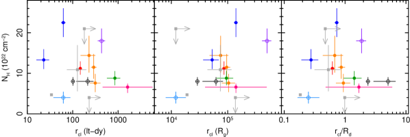
Figure 9: Best-fitting values of $N_{\rm H}$ plotted against inferred radial location $r_{\rm cl}$ in units of light-days (left), in units of gravitational radii $R_{\rm g}$ (center; $R_{\rm g}\equiv GM_{\rm BH}/c^{2}$), and relative to dust sublimation radius $R_{\rm d}$. Filled and open symbols correspond to type I and II objects, respectively. Colors are the same as in Fig. 6.

Finally, we investigate any possible trend between the best-fitting values of peak $N_{\rm H}$ and the inferred values of $r_{\rm cl}$ listed in Table 5, in units of either light-days, $R_{\rm g}$, or $r_{\rm cl}$/$R_{\rm d}$ (Fig. 9). Given the small number of eclipse events, and given that values of $N_{\rm H}$ span only a factor of $\sim$7, we find no robust correlations; inclusion/exclusion of only 1–2 secure or candidate points significantly changes the resulting coefficients and null hypothesis probabilities. Note that the overdensity of eclipse events around 200 light-days (left-hand panel), $8\times 10^{4}R_{\rm g}$ (middle panel), and $\la 1R_{\rm d}$ (right-hand panel) is likely not intrinsic to the sources but mainly caused by our selection function. This figure should thus not be used to derive constraints on the radial distribution of clouds.

Table 5: Inferred cloud distances from the black hole

Source		log($M_{\rm BH}$)		$L_{2-10}$, $L_{\rm ion}$, $L_{\rm Bol}$,	log($\xi$, erg	$r_{\rm cl}$	$r_{\rm cl}$
name	Event	($\rm M_{\odot}$)	Ref.	(erg s-1)	cm s-1)	(light-days)	($10^{4}$ $R_{\rm g}$)	$r_{\rm cl}$/$R_{\rm d}$	Notes
NGC 3783	2008.3	7.47	VP06	43.2, 44.1, 44.4	0	$147^{+11}_{-10}$	$8.6^{+0.7}_{-0.6}$	$0.62\pm 0.04$
	(Full event)
Mkn 79	2003.5	7.72	Pe04	43.3, 44.3, 44.7	0	$229^{+83}_{-79}$	$7.5\pm 2.7$	$0.68\pm 0.24$
	2003.6				0	$290^{+42}_{-35}$	$9.6^{+1.4}_{-1.1}$	$0.86^{+0.13}_{-0.09}$
	2009.9				0	$314^{+91}_{-74}$	$10.4^{+3.0}_{-2.5}$	$0.93^{+0.27}_{-0.22}$
Mkn 509	2005.9	8.19	VP06	44.3, 44.9, 45.2	0	$851^{+255}_{-278}$	$9.5^{+2.9}_{-3.1}$	$1.42^{+0.42}_{-0.46}$	†
MR 2251–178	1996	8.3	W09	44.7, 45.3, 45.6	0	460–5700	4–49	0.5–6.0	†‡
NGC 3227	2000–1	6.88	D10	42.5, 43.0, 43.5	–0.3	$82^{+9}_{-8}$	$19\pm 2$	$0.97\pm 0.11$
					0	$62^{+7}_{-6}$	$14\pm 1$	$0.74\pm 0.05$
	2002.8				0	$23\pm 7$	$5.3\pm 1.6$	$0.28^{+0.08}_{-0.09}$
Cen A	$\sim$2003–4	7.78	R11	41.9, 42.3, 42.9	0	$214^{+70}_{-93}$	$6.2^{+2.0}_{-2.6}$	$5.3^{+1.6}_{-2.1}$	†
	2010–1				0	$101^{+7}_{-6}$	$2.9\pm 0.2$	$2.4\pm 0.2$
NGC 5506	2000.2	7.94	Pa04	43.0, 43.9, 44.3	0	$62^{+26}_{-24}$	$1.2^{+0.6}_{-0.4}$	$0.26^{+0.11}_{-0.08}$
Mkn 348	1996–7	7.18	WZ07	43.0, 44.1, 44.4	0	$432^{+79}_{-73}$	$50\pm 9$	$1.82\pm 0.37$	†
Fairall 9	2001.3 (cand.)	8.41	VP06	43.4, 44.6, 44.8	0	$>$180	$>$1.2	$>0.5$	∗
NGC 3783	2008.7 (cand.)	7.47	VP06	43.2, 44.1, 44.4	0	$>$230	$>$13.7	$>1.0$	∗
	2011.2 (cand.)				0	$127^{+71}_{-52}$	$7.4^{+4.2}_{-3.0}$	$0.54^{+0.30}_{-0.22}$
NGC 3516	2011.7 (cand.)	7.50	D10	43.0, 43.7, 44.2	+2.19	34	1.9	$\sim 0.6$	∗∗
Average for 12 Secure Events		7.63		43.1, 43.8, 44.2		200	8.0	1.0

Estimates of the distance from the central black hole to each eclipsing cloud $r_{\rm cl}$ following $\S$5.2. Uncertainties listed above do not include uncertainty on the ionization parameter $\xi$. Reasonable ranges for log($\xi$) are –1 to +1 for most objects, which translates into factors of 2.5 larger/smaller (for Cen A, values of log($\xi$) ranging from –1 to 0 are plausible; for NGC 3227/2000–1, Lamer et al. (2003) measured log($\xi$) = –0.3–0). $L_{2-10}$ is the 2–10 keV of the hard X-ray power-law component from the long-term time-averaged RXTE spectrum (Rivers et al. 2013). $L_{\rm ion}$ is the 1–1000 Ryd ionizing luminosity; please see $\S 5.2$ for details. $L_{\rm Bol}$ is the bolometric luminosity; please see $\S 5.1$ for details. Luminosities are corrected for all (intrinsic and Galactic) absorption. $R_{\rm d}$ denotes the outer boundary of the “dust sublimation zone” (Nenkova et al. 2008b), i.e., dust residing at distances greater than $R_{\rm d}$ likely does not sublimate, while distances smaller than $\sim\frac{1}{2}-\frac{1}{3}R_{\rm d}$ are expected to be dust-free. Average values (last row) were determined in log space. References for $\rm M_{\odot}$ are: D10 = Denney et al. (2010), Pa04 = Papadakis (2004), Pe04 = Peterson et al. (2004), R11 = References in Rothschild et al. (2011), VP06 = Vestergaard & Peterson (2006), W09 = Wang et al. (2009), and WZ07 = Wang & Zhang (2007).

^†Estimates of $r$ may be lower if peak $N_{\rm H}$ was higher than that measured because either the beginning or end of the eclipse was not covered by monitoring data.

^‡For MR 2251–178, we have only limits to the duration, but no reliable “best estimate.”

^∗Upper limits on $N_{\rm H}$ were used to derive lower limits on $r_{\rm cl}$.

^∗∗Assumed ionization following Turner et al. (2008); see Appendix A.

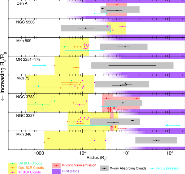
Figure 8: Plot of inferred radial locations of the secure X-ray-absorbing clouds $r_{\rm cl}$, plus inferred radial locations of IR continuum-emitting dust and BLR clouds, in units of $R_{\rm g}$. See Table 16 for details. Sources are ranked in order of increasing $R_{\rm d}$/$R_{\rm g}$. Locations of each of the X-ray absorbing clouds for an assumed ionization value of log($\xi$)=0 are denoted by black points, with the full range obtained with log($\xi$) spanning values from –1 to +1 (with –1 to 0 for Cen A and –0.3 to 0 for NGC 3227/2000–1) indicated by the gray shaded areas. The data point for MR 2251–178 is omitted due to the poor constraints on $t_{\rm D}$ and thus $r_{\rm cl}$. The purple shaded areas denote radial distances expected to contain dust, with the fading purple areas (1.0 down to 0.4$R_{\rm d}$) denoting the “dust sublimation zone.” Known locations of IR continuum emitting dust are plotted in red points, with ranges indicated by pink shaded areas. BLR ranges are indicated by the yellow areas. Green points indicate origins of UV broad emission lines (e.g., He ii, C iv, S iv). Orange points show origins of optical broad emission lines (e.g., Balmer series). Magenta points show origins of IR broad emission lines (e.g., Bracken and Paschen series, He i$\lambda$2.058$\mu$). Locations of Fe K$\alpha$-emitting gas are plotted in cyan. As a reminder, radial locations of these structures may be commensurate but structures may not physically overlap, e.g., the X-ray-absorbing clouds lie on the direct line of sight to the central engine, but emission components may lie off the line of sight.

5.3 A possible double-eclipse event in NGC 3783

The $N_{\rm H}$($t$) and $HR1$ profiles for the NGC 3783/2008.3 event are highly intriguing, as the two spikes suggest two absorption events separated by only 11 d. The fact that, assuming that $\Gamma$ remains constant during this time, $N_{\rm H}$($t$) remains near $4\times 10^{22}$ cm^-2 in between the spikes is also intriguing. No such complex $N_{\rm H}$($t$) profile has been observed for any other AGN to date.

As illustrated in Fig. 10, we model the $N_{\rm H}$($t$) profile in several ways, fitting only bins #5–14 (see Table 7 for bin definition; refers to those bins with non-zero values of $N_{\rm H}$ plus two bins with upper limits before and after). We first test a single uniform-density sphere (gray line), which yields $\chi^{2}/dof$ = 40.1/11=3.65 and underestimates the spikes in $N_{\rm H}$ in bins #9 and #15.

We also fit the profile assuming two independent eclipsing events. We test a profile from two uniform-density spheres (cyan line), and one from two linear-density spheres profile (red line). For the latter, the density profile is $n$($r$) = $n_{\rm max}$(1–$r/R$), where $n_{\rm max}$ is the number density at the center and $R$ is the outer radius of the cloud along the transverse axis (red line). Each cloud’s center point in time space is held frozen at the midpoints of bins #9 or 15. The best-fitting models yield $\chi^{2}/dof$ = 50.2/10=5.02 and 48.9/10=4.89, respectively, and did not correctly fit bin #9 nor the $\sim$2–4 bins between the spikes. We also fit each spike with a phenomenological $\beta$-profile of the form $N_{\rm H}$($t$) = $N_{\rm H,max}\sqrt{1-r/R_{\rm c}}$ (panel c), where $N_{\rm H,max}$ is the column density along a line of sight through the cloud’s center and $R_{\rm c}$ is the core radius (Dapp & Basu 2009). The best fit yields $\chi^{2}/dof$ = 39.5/10=3.95 but still underestimates the middle part of the profile.

Furthermore, the probability that two separate eclipse events could independently occur so close together in time is low: NGC 3783 was monitored for 3.27 yr, had no observations for 1.88 yr, and then was monitored for an additional 7.84 yr. We perform Monte Carlo simulations wherein we assume a 1.0-d grid and we randomly place three eclipses in the 3.27 or 7.84-yr campaigns, and empirically estimate the probability that any two of their peaks can occur $<$15 d apart: only 0.24 per cent. Combined with the fact that $N_{\rm H}$($t$) does not return to zero between the two spikes, the likelihood that the profile is comprised of two independent eclipse events seems low. The addition of a third independent cloud with $N_{\rm H}\sim 4\times 10^{22}$ cm^-2 transiting the line of sight roughly halfway between the maximum transits of the other two would of course yield a good fit to the observed $N_{\rm H}$($t$) profile, but this is statistically highly unlikely ($\sim 5\times 10^{-6}$).

Finally, we model a uniform-density shell (green line in Fig. 10; subtracting a smaller uniform-density sphere from another) to successfully model fit the middle part and the two spikes. The best fit has $\chi^{2}/dof$ = 13.2/9=1.47, with the outer and inner shell boundaries taking $7.5^{+0.5}_{-1.0}$ and $4.5\pm 0.5$ d, respectively, to transit the line of sight. However, we stress that this fit is purely phenomenological; it is not clear how such a structure could be created or survive for long periods in an AGN environment.

We speculate that the observed profile could be caused by two dense clumps with some sort of connecting structure (a dumbbell shape), with parts aligned along the direction of travel across the line of sight. We discuss a possible physical origin for this behavior in $\S$5.4.1.

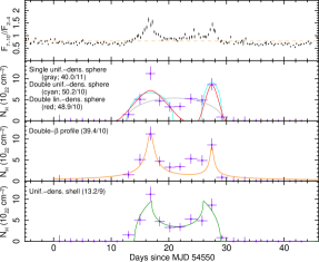
Figure 10: $HR1$ and $N_{\rm H}$($t$) light curves for the NGC 3783/2008.3 event, with its suspected “dual-clump” profile. The solid lines indicate the best-fitting models to the $N_{\rm H}$($t$) profile; we fit only bins #5–14 (those bins with non-zero values of $N_{\rm H}$ plus two bins with upper limits before and after; see Table 7 for bin definition). We test a single uniform-density sphere (gray), a dual uniform-density sphere model (cyan), a dual linear-density-sphere model, a dual $\beta$-profile (orange), and a uniform-density shell (green). Values of $\chi^{2}/dof$ are in parentheses.

5.4 Physical properties of obscuring clouds

We estimate diameters, number densities and masses for each eclipsing cloud using the equations in $\S$5.2 and listed them in Table 6. The average diameter across the sample of secure events is $\sim 0.25$ light-days, with an average number density of $\sim 3\times 10^{8}$ cm^-3. Nenkova et al. (2008b) estimate theoretically that a total of $\sim 10^{4}-10^{5}$ clouds comprises the dusty torus. The mass estimates for individual clouds in Table 6 span $\sim 10^{-8}-10^{-2}\rm M_{\odot}$ with a mean value in log space of $10^{-5.2}\rm M_{\odot}$, thus suggesting a total mass for the clumpy component of the torus (i.e., excluding any thin accretion disk or intercloud diffuse medium) of $\sim 10^{-4}-10^{3}\rm M_{\odot}$. If the torus clouds are produced in a disk wind, then this estimate indicates the maximum mass associated with the outflow. Since the value of $\sim 10^{4}-10^{5}$ clouds quoted above likely refers only to IR-emitting clouds located outside $R_{\rm d}$, this mass refers to clouds lying outside $r_{\rm d}$ only, and also ignores contributions from non-clumpy material such as any intercloud medium (Stalevski et al. 2012).

Table 6: Inferred physical properties of each cloud; inferred size of X-ray-emitting region

Source		Diam.	Diam.	Num. dens., $n$	log(mass)	$D_{\rm X-src}$
name	Event	($10^{14}$ cm)	(light-days)	($10^{8}$ cm-3)	($\rm M_{\odot}$)	($R_{\rm g}$)
NGC 3783	2008.3	$1.3^{+0.7}_{-0.5}$	$0.048^{+0.029}_{-0.018}$	$8.6^{+7.0}_{-3.9}$	$-6.0^{+0.4}_{-0.5}$	$<47$
Mkn 79	2003.5	$2.4^{+2.6}_{-1.5}$	$0.089^{+0.097}_{-0.057}$	$6.0^{+15.9}_{-4.0}$	$-5.4^{+0.5}_{-0.8}$	$<64$
Mkn 79	2003.6	$3.1^{+1.8}_{-1.2}$	$0.11^{+0.07}_{-0.04}$	$3.7^{+3.9}_{-1.9}$	$-5.3\pm 0.5$	$<65$
Mkn 79	2009.9	$2.4^{+2.1}_{-1.3}$	$0.088^{+0.078}_{-0.046}$	$3.2^{+5.5}_{-2.0}$	$-5.7^{+0.4}_{-0.5}$	$<57$
Mkn 509	2005.9	$4.9^{+5.7}_{-3.3}$	$0.18^{+0.21}_{-0.12}$	$1.8^{+4.5}_{-1.1}$	$-5.1^{+0.6}_{-0.9}$	$<46$
MR 2251–178	1996	$0.25-91$	$0.009-3.4$	$0.06-30$	$-7.7$ to $-2.7$	$<310$
NGC 3227	2000–1	$5.8^{+0.3}_{-1.0}$	$0.22^{+0.01}_{-0.04}$	$3.9^{+1.4}_{-0.8}$	$-4.5^{+0.1}_{-0.2}$	$<540$
NGC 3227	2002.8	$0.49^{+0.56}_{-0.31}$	$0.018^{+0.020}_{-0.012}$	$27^{+62}_{-17}$	$-6.9^{+0.6}_{-0.8}$	$<92$
Cen A	$\sim$2003–4	$120^{+60}_{-90}$	$4.5^{+2.3}_{-3.4}$	$0.07^{+0.23}_{-0.03}$	$-2.3^{+0.3}_{-0.2}$	$<2000$
Cen A	2010–1	$26.9^{+0.1}_{-10.1}$	$1.00^{+0.01}_{-0.38}$	$0.30^{+0.24}_{-0.04}$	$-3.6^{+0.1}_{-0.5}$	$<300$
NGC 5506	2000.2	$0.12^{+0.13}_{-0.08}$	$4.3^{+5.8}_{-2.9}\times 10^{-3}$	$34^{+111}_{-23}$	$-8.6^{+0.5}_{-0.9}$	$<1.9$
Mkn 348	1996–7	$20^{+17}_{-10}$	$0.74^{+0.62}_{-0.36}$	$0.90^{+1.17}_{-0.49}$	$-3.5\pm 0.5$	$<1600$
Fairall 9	2001.3	$<4.5$	$<0.17$	$\sim 5-27$	$\sim-6.2$ to $-4.7$	$<12$
NGC 3783	2008.7	$<2.8$	$<0.10$	$\sim 1-5$	$\sim-7.0$ to $-5.9$	$<63$
NGC 3783	2011.2	$0.9^{+1.0}_{-0.6}$	$0.035^{+0.035}_{-0.023}$	$12^{+41}_{-8}$	$-6.4^{+0.4}_{-0.8}$	$<43$
NGC 3516	2011.7	$\sim 11$	$\sim 0.4$	$\sim 0.4$	$\sim-4.6$	$<230$
Average for 12 Secure Events		3.9	0.25	2.6	–5.2	$<120$

Best-estimate values listed here correspond to best-fitting values of $N_{\rm H}$ and values of duration listed in Table 3 and an assumed ionization state of log($\xi$)=0. Uncertainties listed here are based on the uncertainties on observed duration, $N_{\rm H}$, and the ranges of $r_{\rm cl}$ and log($\xi$) listed in Table 5. $D_{\rm X-src}$ denotes inferred upper limits on the size of the X-ray continuum source, assuming that the cloud completely covers the X-ray continuum source. Average values were determined in log space.

Finally, assuming that each eclipsing cloud fully covers the X-ray continuum source behind it, the upper limits on the diameter of the cloud yield inferred upper limits on the size of the X-ray continuum source, $D_{\rm X-src}$. These limits are listed in Table 6 in units of $R_{\rm g}$. Among the secure events, the limits are as low as a few tens of $R_{\rm g}$ for NGC 3783, Mkn 79, and Mkn 509, and even as low as $2R_{\rm g}$ in the case of NGC 5506.

The X-ray continuum in Seyferts is generally thought to originate via inverse Compton scattering of the soft UV photons from the accretion disk by hot electrons in a compact corona, possibly located in the innermost accretion disk or at the base of a jet (e.g., Haardt et al.  1997; Markoff et al. 2005). X-ray microlensing analysis of distant quasars typically yields upper limits on the size of the X-ray corona of $\sim 10R_{\rm g}$ (e.g., Chartas et al. 2012, Chen et al. 2012, and references therein). Recent results using X-ray reverberation lags imply sizes of a few to $\sim 10$ $R_{\rm g}$ (Reis & Miller 2013). Geometrical limits from absorption variability in NGC 1365 typically yield $D_{\rm X-src}\la 30-60R_{\rm g}$ (Risaliti et al. 2007, 2009b). Our estimates of $D_{\rm X-src}$ are consistent with these studies.

5.4.1 Exploring the range in observed density profiles

We speculated in $\S$5.3 that the unusual density profile of the NGC 3783/2008.3 event could be caused by the cloud having a dumbbell shape. Even more speculatively, perhaps this structure is a cloud that is in the process of getting torn in half. As pointed out by Krolik & Begelman (1988), the self-gravity of a single cloud in the vicinity of a supermassive black hole is not highly effective against tidal shearing, and clouds can get significantly stretched out within an orbit. Resistance to tidal shearing requires that the size of the cloud is limited to $\la D_{\rm shear}=10^{16}N_{\rm H,23}r_{\rm pc}^{3}M_{7}^{-1}$ cm, where $N_{\rm H,23}=N_{\rm H}/10^{23}{\rm cm}$, $r_{\rm pc}$ is the distance from the black hole to the cloud, and $M_{7}=M_{\rm BH}/(10^{7}\rm M_{\odot})$ (Elitzur & Shlosman 2006). For NGC 3783/2008.3, $D_{\rm shear}\sim 7\times 10^{12}$ cm, a factor of $\sim 1/18$ times the inferred cloud diameter $D_{\rm cl}$, so the possibility of tidal shearing seems plausible. In fact, for all secure eclipse events, we obtain values of $D_{\rm cl}/D_{\rm shear}$ spanning 2.3–350, with an average value (in log-space) of 26, suggesting that many of these clouds’ sizes put them at risk of being tidally disrupted or sheared.

The unusual density profile could also be consistent with models wherein torus clouds may be in the form of clumpy winds, as opposed to compact, discrete clouds, originating at the accretion disk. These winds may be magnetohydrodynamic (MHD) driven (e.g., Konigl & Kartje 1994; Fukumura et al. 2010), with local column densities that can be consistent with values measured in this paper. Other models feature IR radiation-driven winds (Dorodnitsyn & Kallman 2012; Dorodnitsyn et al. 2012): UV/X-ray photons are reprocessed into IR thermal emission in the torus, and IR radiation pressure vertically drives dust grains. Moderately Compton-thick flows are possible at distances of $\ga$1 pc from the black hole (if our assumption about Keplerian motion is not valid, then distance estimates for our clouds may be in error). The models generally assume that clouds’ self-gravity is negligible. Similarly, Czerny & Hryniewicz (2011) proposed a turbulent, dusty, disk wind as the origin for the low-ionization region of the BLR: clouds rise from the disk, intense external radiation heats the gas and dust sublimates. In all these models, the torus is highly dynamic and can feature cloud motions perpendicular to the disk (including failed winds), and thus not strictly Keplerian. In any case, the $N_{\rm H}$($t$) profile of the NGC 3783/2008.3 event can thus also be explained via a non-homogeneous mass outflow, featuring two overdensities that crossed the line of sight 11 d apart.

However, the profile of NGC 3783/2008.3 contrasts with three of the other eclipse events that have $N_{\rm H}$($t$) profiles that are also well resolved in time but are symmetric and centrally peaked: NGC 3227/2000–1 and Cen A/2010–1, observed with RXTE, and SWIFT J2127.4+5654 (Sanfrutos et al. 2013). Such profiles pose a challenge to MHD/IR-driven wind models. For example, the IR-driven winds of Dorodnitsyn et al. (2012) suggest that $\Delta$$N_{\rm H}$/$N_{\rm H}$ is typically $\sim$ a few (less than the factors we observe). In addition, such winds are inferred to originate $\sim 1-3$ pc from the black hole, farther than the distances inferred for our observed eclipses.

In summary, the self-gravity of these clouds likely dominates over any tidal shearing/internal turbulence, presenting a challenge to the expectation that clouds are easily tidally sheared. In these cases, one or more of the assumptions that go into the calculations of $D_{\rm cl}$ or $D_{\rm shear}$ may be wrong. Alternately, some other physical process may prevent clouds from shearing, e.g., confinement of these clouds by external forces (e.g., gas pressure from the ambient medium, external magnetic fields; Krolik & Begelman 1988) may be important.

5.5 Implications for clumpy-absorber models

Clumpy torus models have found a lot of observational support, particularly from recent IR observations. For example, smooth-density torus models always predict that the silicate features at 9.7 and 18$\mu{\rm m}$ will be in emission for pole-on viewing and in absorption for edge-on viewing. However, samples of mid-IR spectra of type I Seyferts can exhibit silicate features spanning a range of emission and absorption (see Hao et al. 2007 for a sample obtained with Spitzer); type IIs generally show only weak absorption but a few can show emission (Sturm et al. 2005; Hao et al. 2007). Nenkova et al. (2008b) and Nikutta et al. (2009) demonstrate that the clumpy-torus models are consistent with these observations and can explain mismatches between the optical classification and the expected behavior of the silicate features. Clumpy-torus models predict nearly isotropic mid-IR continuum emission and anisotropic obscuration, as generally observed (e.g., Lutz et al. 2004; Horst et al. 2006). Finally, clumpy tori have been predicted to host both hot and cooler dust in close proximity to each other (Krolik & Begelman 1988), in contrast to smooth-density tori. Recent IR interferometric observations indeed do affirm such a co-existence of hot (800 K) and cooler ($\sim 200-300$ K) dust components in nearby AGN (Jaffe et al. 2004; Poncelet et al. 2006; Tristram et al. 2007; Raban et al. 2009).

In this subsection, we derive the first X-ray constraints on the Clumpy model parameters, thus obtaining constraints in a manner independent from IR SED fitting. We caution, however, that there may not be an exact correspondence between constraints derived from the two methods, since IR emission arises only from dusty clouds outside the DSZ while our X-ray clouds can be dust free. The clumpy-torus models are generally defined using the following free parameters: $\tau_{\rm V}$ is the $V$-band optical depth of single clouds; usually, all clouds are assumed to have identical values of $\tau_{\rm V}$. The radial extent of the dusty torus is characterized by $Y$, the ratio of the outer radial extent of clouds to the dust sublimation radius $R_{\rm d}$. $\hbox{${\cal N}_{i}$}(\theta)$ is the average number of clouds along a radial line of sight that is an angle $\theta$ from the equatorial plane. Assuming a Gaussian distribution, $\hbox{${\cal N}_{i}$}(\theta,\sigma,\hbox{${\cal N}_{0}$})=\hbox{${\cal N}_{0}$}\exp(-(\theta/\sigma)^{2})$, where ${\cal N}_{0}$ is the average number of clouds along a radial line of sight in the equatorial plane (typically 5–15), and $\sigma$ parametrizes the angular width of the cloud distribution. The index $q$ describes the radial dependence of the average number of clouds per unit length, $\hbox{${\cal N}_{C}$}(r,q)\propto r^{-q}$. The inclination angle of the system is $i\equiv 90\degr-\theta$, defined such that $i=0$ ($\theta=90\degr$) denotes a system with its equatorial plane in the plane of the sky.

The predicted shape of the IR SED is sensitive to all of these parameters. Ramos Almeida et al. (2009, 2011; hereafter RA09 and RA11) have successfully fit the mid-IR spectra of $\la 20$ AGN with Clumpy torus models and the BayesClumpy tool (Asensio Ramos & Ramos Almeida 2009). There are only three sources in our eclipse sample that overlap with the samples of RA09 and RA11 (NGC 3227, Cen A, and NGC 5506). In the following we attempt to focus on comparing our derived parameter constraints for the type I/II classes as opposed to for individual objects.

$\bullet$ $\tau_{\rm V}$: we can translate our inferred values of $N_{\rm H}$ for individual clouds into values of $\tau_{\rm V}$, which we can then compare to those values typically used in the Clumpy model fitting. From the “secure” clumps we observe, $\Delta$$N_{\rm H}=4-26\times 10^{22}~{}{\rm cm}^{-2}$, with values spanning very similar ranges for both type Is/IIs. Using the Galactic dust/gas conversion ratio, $N_{\rm H}=A_{\rm V}{\rm(mag)}\times 1.8\times 10^{21}{\rm cm}^{-2}$ (Predehl & Schmidt 1995), these values translate to $A_{\rm V}=22-144$ mag, or $\hbox{$\tau_{\rm V}$}=20-132$. The Clumpy models use one value of $\tau_{\rm V}$ per object/spectrum to represent the weighted average value across all clouds in that object. In contrast, we probe 1–3 individual clouds per object. Subject to small-number statistics, we can therefore test both the inter-object scatter of $\tau_{\rm V}$ values, as well as the scatter from cloud to cloud in one given source. From general theoretical considerations, Nenkova et al. (2008b) suggest that $\tau_{\rm V}$ be typically 30–100. RA11, who use the entire Clumpy database of models in their IR SED fitting, estimate values of 40–140 for type Is and 5–95 for type IIs. Alonso-Herrero et al. (2011), with the same approach but different sources, find $\tau_{\rm V}$ = 105–146 (type Is) and 49–130 (type IIs). These IR-derived ranges are fully consistent with our X-ray based values. In contrast to the above studies, we find no evidence for different cloud optical depths between type I and II sources.

Three of our sources are also present in the IR samples of RA11 and Alonso-Herrero et al. (2011). In two of these (Cen A and NGC 3227) our X-ray constraints agree very well with the IR ones. However, our value for NGC 5506 is smaller than that in RA11 by a factor of $\sim 2$ and smaller than that of Alonso-Herrero et al. (2011) by $\sim 5$. For our sources with multiple eclipsing events, the measured scatter in $N_{\rm H}$ or $\tau_{\rm V}$ is very low, always $<$2. It seems then that assuming a single average value of $\tau_{\rm V}$ for all clouds in a given Clumpy model is justified.

$\bullet$ $Y$: the IR SED modeling and interferometry indicate the presence of dusty clouds out to $Y\sim 20-25$ (e.g., RA11), although emission from beyond this radius may be difficult to separate from the surrounding host galaxy emission, especially for emission longer than $\sim 10\hbox{$\mu{\rm m}$}$. Our inferred locations of the X-ray-absorbing clouds cover out to $Y\sim 20$, in agreement with the IR observations. It should be noted though that clouds at much larger distances from the black hole might exist, but would only be detectable with even longer sustained X-ray monitoring campaigns of a larger number of targets.

$\bullet$ $\sigma$, $i$ ($\theta$) and ${\cal N}_{0}$: we observe eclipse events in type I objects, and derive non-zero values of $P_{\rm ecl}$. If it is the case that all type Is are oriented relatively face-on, then clumpy-torus models featuring sharp-edged tori are strongly disfavored, while models featuring a gradual decline of cloud number when moving away from the equatorial plane are favored (see left- and right-hand panels of Nenkova et al. 2008b, Fig. 1, respectively). IR SED fitting likewise disfavors sharp-edged tori, which would produce a dichotomy in the SED shapes that is not observed (Nenkova et al. 2008b).

We can derive our constraints on $\sigma$ and ${\cal N}_{0}$ assuming that an observed baseline level of absorption $N_{\rm H,base}$ corresponds to an average of ${\cal N}_{i}$ clouds along the line of sight ($\hbox{${\cal N}_{i}$}=0$ in the case of sources normally lacking X-ray obscuration). We also assume that an eclipse denotes $\hbox{${\cal N}_{i}$}\rightarrow\hbox{${\cal N}_{i}$}+1$. In the case of Cen A, to repeat the exercise from Rothschild et al. (2011) and Rivers et al. (2011b), $\Delta$$N_{\rm H}$/$N_{\rm H,base}\sim 3$, suggesting $\hbox{${\cal N}_{i}$}\sim 2$. From IR interferometry, Burtscher et al. (2010) model a best-fitting value for the torus inclination of $i=63\degr$, or $\theta=27\degr$. The median value for $\sigma$ modeled by RA11 was $\sigma=20\degr$; in order to agree with this value of $\sigma$, one needs $\hbox{${\cal N}_{0}$}=12$.

In both cases of NGC 5506 and Mkn 348, $\Delta$$N_{\rm H}$/$N_{\rm H,base}\sim 2$, suggesting $\hbox{${\cal N}_{i}$}\sim 1$. Due to the absence of external information on $i$, we can only derive constraints on the ratio $\theta/\sigma$. If we assume that $\hbox{${\cal N}_{0}$}=10$, $\theta/\sigma$ = 1.52. That is, if such a system is inclined relatively edge-on ($\theta\rightarrow 0$), as is commonly suspected for type IIs, then $\sigma$ must be rather small, indicating a tightly flattened distribution. Otherwise, the inclination of the system would have to deviate more from an equatorial view. This exercise assumes that all obscuring material along the line of sight is in the form of clouds. If the baseline absorption $N_{\rm H}$ is not due to clouds (see $\S$5.6), then $\hbox{${\cal N}_{i}$}\sim 0$, suggesting that the inclination of the system may not be close to edge-on, and/or that $\sigma$ is relatively small in these systems. A similar condition, $\hbox{${\cal N}_{i}$}\sim 0$, applies to sources normally lacking X-ray absorption, e.g., the type I objects in our sample.

For a Clumpy torus the probability of the AGN being obscured – a single dust cloud along the line of sight is sufficient – is given by

$$\hbox{$P_{\rm obsc}$}(\hbox{${\cal N}_{0}$},\hbox{$\sigma$},i)=1-\exp\left\{-\hbox{${\cal N}_{0}$}\cdot\exp\left\{-\left(\frac{90-i}{\sigma}\right)^{\!\!\!2}\right\}\right\}$$ (2)

(e.g., Nenkova et al. 2008b; Nikutta et al. 2009). The argument to the outer exponential is the (negated) number of clouds along the line of sight ${\cal N}_{i}$, thus $\hbox{$P_{\rm obsc}$}=1-\exp\{-\hbox{${\cal N}_{i}$}\}$. We can attempt to constrain the Clumpy parameters ${\cal N}_{0}$, $\sigma$, and $i$ by identifying ranges of $P_{\rm obsc}$ consistent with our X-ray monitoring data. In Fig. 11 we plot $P_{\rm obsc}$ as a function of 2 of the 3 parameters, with each row of panels sampling the third parameter. The scale is linear (see color bar). In each panel we overplot as contour lines $\overline{P_{\rm ecl}}$, the inferred values of the probability to catch an AGN while being obscured by a torus cloud, as computed in $\S$4.3 (Table 4). The solid lines correspond to the minimum and maximum values of $\overline{P_{\rm ecl}}$, and dotted lines are best-estimate values. The white lines thus outline, given the data and the selection function, the range of permitted values of $P_{\rm obsc}$ for type I objects, and the black lines trace the allowed range of probabilities for type II objects. The dotted lines are the best-estimate values of $P_{\rm obsc}$.

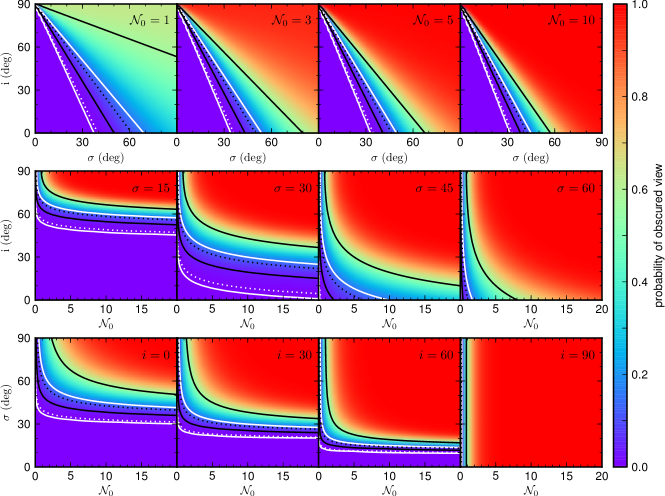
Figure 11: Clumpy parameter constraints based on the theoretical probability $P_{\rm obsc}$ to see the AGN obscured by torus clouds. The obscuration probability is rendered as a color scale in each panel (see color bar). The top panels show $P_{\rm obsc}$ as a function of torus angular width $\sigma$ and viewing angle $i$ for four different values of ${\cal N}_{0}$. The other two combinations of the three parameters that enter $P_{\rm obsc}$ are depicted in the middle and bottom rows. Overplotted as contour lines in each panel are the inferred ranges of $\overline{P_{\rm ecl}}$ that are compatible with our X-ray monitoring data (see Table 4). White and black solid lines outline the compatible ranges for type I and II objects, respectively. The dotted lines indicate best estimates in both cases.

These inferred minimal and maximal probabilities outline the parameter ranges permissible by our extensive monitoring programmes. Given the observed (and not observed!) eclipsing events, any torus parameters which lie outside the enclosed ranges are unlikely to be found in real sources. We remind the reader, however, that the probability values $\overline{P_{\rm ecl}}$ we derived in $\S$4 refer only to lowly-ionized/neutral, full-covering clouds with $N_{\rm H}\ga 10^{22}$ up to $\sim 10^{25}$ cm^-2. When eclipses are due to clouds with higher ionizations and/or lower column densities, and partial-covering events, the values will be higher. Since three parameters (${\cal N}_{0}$, $\sigma$, $i$) affect $P_{\rm obsc}$ with some mutual dependence on each other, it is not straightforward to give one-dimensional ranges of excluded parameter values. However, for physically reasonable values some constraints can be given ad hoc. For instance, if ${\cal N}_{0}$ is between 5 and 15 (see, e.g., Nenkova et al. 2008b), it is clear from Fig. 11 (bottom row) that $\sigma$ must be smaller than $\approx 45\hbox{${}^{\circ}$}$ (even for type II sources); only at the most pole-on viewing angles, $\sigma$ can be slightly higher. Similarly, if, for instance, $\sigma$ is secured by external information, for the reasonable range of ${\cal N}_{0}$ the permitted viewing angles $i$ are very well-constrained (see middle row of Fig. 11). Not surprisingly, the permissible parameter values in type II sources are on average higher than in type I sources, because $P_{\rm obsc}$ increases when any of the three (${\cal N}_{0}$, $\sigma$, or $i$) grows. There is some overlap, however, and is most likely indicative of ”intermediate” types of AGN.

Overall, Fig. 11 shows that whenever one of the three parameters can be secured by other means, the other two allow only relatively narrow ranges. In practice, external information is sometimes available, for instance on the orientation of the AGN system from radio jets or from narrow-line ionization cones, and can be used to infer the two other parameters. We are not attempting a full Bayesian parameter inference on the torus parameters here. Suffice it to say here that our results as depicted in Fig. 11 translate into information on the priors $P(\bm{\theta})$ of the Bayesian inference problem $P(\bm{\theta}|D)\propto P(\bm{\theta})\cdot P(D|\bm{\theta})$. Here $\bm{\theta}=(\hbox{${\cal N}_{0}$},\hbox{$\sigma$},i,\ldots)$ is the vector of model parameters to be estimated, $P(D|\bm{\theta})$ is the likelihood that a set of parameter values generates a model compatible with the data, and $P(\bm{\theta}|D)$ is the full parameter posterior (also called inverse probability). Faced with perfect ignorance of the distribution of parameter values before modeling, uniform priors are often assumed. If there is independent knowledge available on some parameters it is imperative to incorporate this information into the Bayesian priors. For example, if the orientation of an AGN was known to be pole-on, one could assume a narrow Gaussian shape on the prior of $i$. We presume that then the Bayesian inference process would yield parameter intervals for ${\cal N}_{0}$ and $\sigma$ commensurate with the lower-left panel of Fig. 11.

The $P_{\rm obsc}$ function transitions quite steeply from very low to very high probabilities. Our derived probability ranges (see Table 4) typically bracket most of the transition region, and also exclude a large fraction of the parameter space that corresponds to extremely low or extremely high $P_{\rm obsc}$. We presume that a source such as NGC 1365, aligned so that ${\cal N}_{i}$ (average number of clouds along the line of sight) is $\approx 1$, would be just at the high end, or slightly above, of the type II region encompassed by the black lines in Fig. 11.

5.6 Can clumpy-torus models be applied to type II objects?

As detailed in Appendix A and summarized in $\S$3, RXTE provided sustained long-term monitoring for durations $\geq$0.6 yr for nine type II objects. In eight of them, $HR1$ is consistent with remaining constant for durations $\geq$0.6 yr (we include the 2011 monitoring of Mkn 348 here). This constancy comes despite variations of typical factors $\sim 2-4$ in 2–10 keV continuum flux. For example, excluding the $\la$1-d event in NGC 5506, there are no strong variations in $HR1$ (sustained trends above 2$\sigma$ and/or $\sim 1.5\times\langle HR1\rangle$) lasting longer than 1 d for a period of 8.39 yr. Each of these sources routinely show evidence for the presence of absorbing gas with $N_{\rm H}\sim 10^{21-23}$ cm^-2 in their X-ray spectra, suggesting a baseline level of absorption $N_{\rm H,base}$ that is consistent with being constant. Using $HR1$ and its distribution, and assuming for simplicity that $\Gamma$ remains constant for each object throughout the monitoring, we estimate the maximum value of $\Delta$$N_{\rm H}$ possible without significantly varying $HR1$. Those values are listed in Table 15, and for the brightest and best-monitored objects is typically $\sim 1-4\times 10^{22}$ cm^-2.

REN02 claim typically 20–80 per cent variations in $N_{\rm H}$ in most of their sample of type II objects, using individual observations from multiple X-ray missions spanning $\sim$25 yr. In this paper, we rely on measurements from one instrument only, and so we do not face systematic uncertainties associated with cross-calibration between various X-ray missions or with fitting spectra data over different bandpasses. For our eight type IIs, we can rule out variations above $\sim 20-30$ per cent for IRAS 04575–7537 and Mkn 348 (2011 monitoring only), and variations above $\sim 50-60$ per cent for NGC 1052, NGC 4258, and NGC 5506.

In the context of the clumpy-torus paradigm, having a non-zero value $N_{\rm H,base}$ requires a non-zero number of clouds along the line of sight at all times, with the observed value of $N_{\rm H,base}$ being the sum of the values of $N_{\rm H}$ for the individual clouds. Assuming that all clouds have the same physical characteristics ($n$, $N_{\rm H}$, etc.), the measured long-term constancy in $N_{\rm H,base}$ would require that the number of clouds along the line of sight ${\cal N}_{i}$ either remain constant for many years or is sufficiently large such that the addition/subtraction of one cloud intersecting or transiting along the line of sight does not change the total measured value of $N_{\rm H}$ by a detectable amount. However, with most clouds modeled with Clumpy having $\tau_{\rm V}\sim 30-100$, which corresponds to $N_{\rm H}\sim 6-20\times 10^{22}$ cm^-2 assuming the Galactic dust/gas ratio, values of $N_{\rm H,base}$ of $10^{22}-10^{23}$ cm^-2 imply that ${\cal N}_{i}$ cannot be more than a few.

We can explore if it is feasible to have the observed duration for each source correspond to a period where ${\cal N}_{i}$ remains constant. That is, we assume that all cloud contributing to the total observed value of $N_{\rm H}$ remain in the line of sight for the duration, and we assume for simplicity that every cloud has identical $N_{\rm H}$. We also assume that every such cloud is $D_{\rm cl}$ = 1 light-day in diameter and on Keplerian orbits. Furthermore, we assume that the fastest velocity (closest to the black hole) cloud has just started to transit the line of sight when the long-term monitoring began, and that the cloud begins to leave the line of sight just when the monitoring ends. In the case of NGC 5506 ($M_{\rm BH}=10^{7.94}\rm M_{\odot}$), an 8.39-year-long transit by such a cloud would require it to be located at least $r_{\rm cl}=GM_{\rm BH}(t_{\rm d}/D_{\rm cl})^{2}$ = 39 pc from the black hole. For NGC 1052 ($M_{\rm BH}=10^{8.19}\rm M_{\odot}$; Woo & Urry 2002), a 4.56-year transit would place it $\geq 20$ pc from the black hole. For NGC 4258, ($t_{\rm d}$=6.81 yr, 2005 March – 2011 December; $M_{\rm BH}=3.9\times 10^{7}\rm M_{\odot}$, Miyoshi et al. 1995; Herrnstein et al. 1999), $r_{\rm cl}\geq$ 11 pc. A cloud diameter of 0.1 light-days, also a feasible value given the range listed in Table 6, would yield values of $r_{\rm cl}$ an order of magnitude higher.

The clumpy-torus models typically assume that clouds cannot exist in large numbers out to several tens of $r_{\rm d}$, or very roughly 10, 5 and 0.5 pc for NGC 5506, NGC 1052, and NGC 4258, respectively. In these objects, it is thus not very likely that the same clouds used in the Clumpy models can also be responsible for the non-variable baseline level of absorption.

Furthermore, Lamer et al. (2003) and Rivers et al. (2011b) demonstrated that the transiting clouds responsible for the NGC 3227/2000–1 and Cen A/2010–1 events were non-uniform, with a number density increasing towards the center. If it were the case that these two clouds were representative of all AGN clouds in terms of their density profiles, then any single cloud moving across the line of sight should produce a secular variation in observed $N_{\rm H}$ and $HR1$. However, we find no evidence for any strong secular trend in any type II object, to the limits indicated by Table 15. In addition, a transiting spherical cloud with a constant column density profile would require $n$ to decrease as one goes from the cloud edge to the center.

We conclude that it is difficult for clumpy-torus models to satisfactorily explain the constancy of $N_{\rm H,base}$, especially in the cases of the few longest-monitored and X-ray brightest type II objects observed with RXTE.

It is thus more likely that $N_{\rm H,base}$ arises in a non-clumpy, highly-homogeneous (to within the above $\Delta$$N_{\rm H}$ limits) medium; such a medium could be located at any radial location along the line of sight, subject to restrictions from the medium’s ionization parameter. That is, the cloud responsible for the $\la 1$-d eclipse in NGC 5506 and the material responsible for $N_{\rm H,base}\sim 2\times 10^{22}$ cm^-2, for instance, are likely physically separate entities. One possibility to explain $N_{\rm H,base}$ is a smooth, relatively low-density, dusty intercloud medium in which the relatively higher density clouds are embedded (Stalevski et al. 2012). To be consistent with the approximate range of baseline values of $N_{\rm H}$ typically measured in type IIs’ X-ray spectra ($0.3-30\times 10^{22}$ cm^-2), the intercloud medium could have values of $\tau_{\rm V}\sim 1.6-160$ or $\tau_{10\micron}\sim 0.07-7$. However, we do not see evidence for such a medium in type I AGN.

Another possibility we explore is X-ray-absorbing gas distant from the black hole and associated with the host galaxy, as has been suggested e.g., by Bianchi et al. (2009) for NGC 7582. For example, dust lanes/patches associated with the host galaxy are considered a candidate for the obscuration of BLR lines in some systems (Malkan et al. 1998).

With the exception of Cen A (see $\S$5.6.1), we rely on Shao et al. (2007) and Driver et al. (2007), who derive the inclination dependence of dust extinction for disk-dominated galaxies. In the optical bands, the extinction is typically $\la 1-2$ mag, derived over a range of inclination angles from face-on to nearly edge-on ($i\sim 80-85\degr$), corresponding to a maximum $N_{\rm H}\sim 4\times 10^{21}$ cm^-2 for a nearly edge-on disk. If the obscuring dust is distributed uniformly throughout the disk of the host galaxy, then such a component may explain relatively low observed values of $N_{\rm H,base}$ in, for instance, NGC 2992 ($N_{\rm H,base}\sim 4\times 10^{21}$ cm^-2) with the disk component of its host galaxy oriented close to edge-on (Jarrett et al. 2003). However, for objects with host disk inclinations far from edge-on (e.g., NGC 4258 and Mkn 348: Hunt et al. 1999; Jarrett et al. 2003) and/or for objects with $N_{\rm H,base}\sim$ a few $\times 10^{22}$ cm^-2 and higher, it is difficult for such a distribution of dust to be associated with $N_{\rm H,base}$. Of course, we cannot rule out the possibility of having more concentrated regions of gas lying along the line of sight not associated with the large-scale disk structure (such as a Giant Molecular Cloud). Dust-free X-ray-absorbing gas in any of these configurations is also a candidate.

A final possible explanation for constancy in $N_{\rm H}$ can be, as mentioned above, the presence of a large number of low-density clouds, with ${\cal N}_{i}$ remaining nearly constant. However, this would require each cloud to have $N_{\rm H}\ll 10^{22}$ cm^-2. Such values contrast with those used by Nenkova et al. (2008b), RA09, RA11, and the values measured in this paper, but such clouds are not physically implausible. Contributions from such clouds, if they are dusty, to the total IR emission are negligible. However, the sum of many clouds along the line of sight that each have $N_{\rm H}\ll 10^{22}$ cm^-2, be they dusty or dust-free, could yield appreciable X-ray absorption.

5.6.1 A small dip in $N_{\rm H,base}$ in Cen A

Up to this point, our discussion of the baseline level of X-ray obscuration in type IIs has centered on constant (to within our sensitivity limits) values of $N_{\rm H,base}$. However, $N_{\rm H,base}$ for Cen A warrants more attention in light of the small dip in early 2010.

The famous dust lane crossing the host elliptical of Cen A supplies 3–6 mag. of optical extinction (Ebneter & Balick 1983), corresponding to $\sim 5-10\times 10^{21}$ cm^-2, far short of observed values of $N_{\rm H,base}\sim 1-2\times 10^{23}$ cm^-2. It is generally accepted that a more compact and higher density distribution is responsible for observed values of $N_{\rm H}$ in X-ray spectra of Cen A.

One possibility is that we have witnessed one cloud leaving the line of sight followed by another cloud entering the line of sight two months later. Best-fitting values of $N_{\rm H}$($t$) indicate a drop from $21.7\pm 0.9$ to $18.6^{+0.9}_{-0.8}$ and returning to $N_{\rm H}$($t$) $=21.9\pm 0.7\times 10^{22}$ cm^-2. These values suggest a scenario in which ${\cal N}_{i}$ dropped temporarily from $\sim$ 7 to 6, with each cloud contributing $\Delta$$N_{\rm H}\sim 3\pm 1\times 10^{22}$ cm^-2, or less than half the column inferred to exist for the clouds causing the 2003–2004 and 2010–2011 increases in total $N_{\rm H}$. If all these clouds are part of the same clumpy structure and have a common origin, then the assumption of each cloud in a given AGN having exactly uniform values of $N_{\rm H}$ is an oversimplification. $N_{\rm H}=3\pm 1\times 10^{22}$ cm^-2 is not an implausible value for a cloud, and only a factor of 2–3 less than that found for other clouds detected in our sample.

$N_{\rm H,base}$ in Cen A could also be attributed to non-clumpy, spatially-extended material that is not entirely homogeneous; perhaps this component can be associated with an intercloud medium. Here, $N_{\rm H,base}$ is usually $\sim 21.8\times 10^{22}$ cm^-2, but there exists an underdense region with $\Delta$$N_{\rm H}=-3\times 10^{22}$ cm^-2 that transited the line of sight in 2010. Assuming an arbitrary distance to the black hole of 100–200 light-days (the location of the absorbing clouds as per $\S$5.2), the $\sim$80-d duration of the dip implies that the underdense region is on the order of half a light-day across.

Longer-term variability in $N_{\rm H,base}$ may also exist: Rothschild et al. (2011) measured values of $14-19\times 10^{22}$ cm^-2 during the 1996–2009 RXTE observations, excluding the 2003–2004 points. Hopefully, future X-ray monitoring will further resolve the variability in $N_{\rm H,base}$ and allow us to discriminate among the above scenarios.

6 SUMMARY

The AGN community is in the process of shifting away from quantifying emission and absorption processes in Seyferts by modeling circumnuclear gas via a homogeneous, Compton-thick “donut” morphology. Instead, a new generation of models describe the torus via distributions of numerous individual clouds, usually preferentially distributed towards the equatorial plane. Often, the clouds are embedded in some outflowing wind from the cold, thin accretion disk that feeds the black hole. Observational support for these models so far has come mainly from fitting IR SEDs in small samples of Seyferts. However, a statistical survey of the environment around supermassive black holes has been needed to properly constrain parameter space in the clumpy-absorber models.

We present the first such survey, the longest AGN X-ray monitoring study to date. Our survey quantifies line-of-sight X-ray absorption by clouds that transit the line of sight to the central engine. Our goals are to assess the relevance of clumpy-torus models as a function of optical classification by exploring absorption over a wide range of length scales (both inside and outside the dust sublimation zone), and to explore links between X-ray absorbers, IR-emitting dusty clouds, and the BLR.

We use the vast public archive of RXTE observations of AGN. The archive features a wide array of sustained monitoring campaigns that make us sensitive to variability in line of sight absorption over a high dynamic range of timescales spanning from 0.2 d to 16 yr. Our final sample consists of 37 type I and 18 Compton-thin-obscured type II Seyferts and totals 230 “object-years,” the largest ever available for statistical studies of cloud events in AGN on timescales from days to years.

We use hardness ratio light curves to identify potential eclipse events, and attempt to confirm the events with follow-up time-resolved spectroscopy. We are sensitive to full-covering, neutral or lowly-ionized clouds with columns densities $\ga 10^{22}$ up to $\sim 10^{25}$ cm^-2. Our results are thus complementary to those derived with $\sim$1 d long-look observations using missions with Chandra, XMM-Newton, and Suzaku.

Our primary results are as follows:

$\bullet$ We find 12 “secure” X-ray absorption events in eight Seyferts (confirmed with spectral fitting) plus four “candidate” eclipses in three Seyferts. As four eclipse events were published previously (NGC 3227/2000–1, Cen A/2003–4, Cen A/2010–1, and Mkn 348/1996–7), we triple the number of events detected in the RXTE archive. The events span a wide range in duration, from $\la 1$ d to over a year. We model the eclipsing clouds to have column densities spanning $4-26\times 10^{22}$ cm^-2. Importantly, we do not detect any full-covering clouds that are Compton thick, although if such clouds are partial-covering clouds then our experiment would not be highly sensitive to them.

$\bullet$ We derived the probability to catch a type I/II source undergoing an eclipse event that has any duration between 0.2 d and 16 yr, taking into account the inhomogeneous sampling in our X-ray observations. For type Is, it is 0.006 (conservative range: 0.003–0.166); for type IIs, 0.110 (0.039–0.571). Our uncertainties are conservative, as they take into account our selection function, candidate eclipse events in addition to the secure ones, uncertainties in the observed durations, and uncertainties in the contributions of individual objects’ sampling patterns to our total sensitivity function. As a reminder, these values indicate the probability to observe a source undergoing an eclipse event (of any duration $t_{\rm D}$ between 0.2 d and 16 yr) due only to a cloud passage through the line of sight, and are independent of long-term constant absorption, e.g., associated with gas in the host galaxy. We conservatively estimate the upper limit to observe a Compton-thick eclipse event (with 0.2 d $<t_{\rm D}<$ 16 yr) to be $<$0.158 or $<$0.520 in type I and II objects, respectively. To repeat the caveat from $\S 4$, these probabilities refer only to eclipses by full-covering, neutral or lowly-ionized clouds with column densities $\ga 10^{22}$ up to $\sim 10^{25}$ cm^-2; when one considers the full range of clouds (larger range of $N_{\rm H}$, partial-covering clouds, wider range of ionization) the resulting probabilities will almost certainly be higher.

Although subject to low number statistics, our observations indicate differences in the distributions of observed eclipse event durations and probabilities for type I and II objects. The type I objects have $\sim 4$ times as many campaigns and twice the number of targets as the type IIs, but despite this, we do not detect eclipse events with durations longer than 100 d (although we cannot rule this out for the poorly-constrained event in MR 2251–178). If it were the case that eclipses with durations of $\sim$hundreds of days occurred in type Is with the same frequency density as in type IIs, then the monitoring campaigns on the type Is should have detected them. This implies that we are ”missing” clouds in type Is along the line of sight at radial distances of $\ga$ a few $\times 10^{5}R_{\rm g}$. This does not necessarily imply intrinsic differences in the cloud distributions of between type Is and IIs, just potential differences along the line of sight.

Despite the generally low probabilities of observing an eclipse, 4/10 objects show secure or candidate eclipse events multiple times. Perhaps the system is close to edge-on, and/or the total number of clouds is very high in these objects. If this is the case, then an object for which an eclipse has been detected has a higher chance of showing an additional eclipse compared to sources with no eclipses so far. In addition, perhaps there exists some dispersion between the averaged derived probabilities of cloud eclipses for a class of objects and the probabilities for individual objects.

$\bullet$ We see no obvious dependence of the likelihood to observe eclipses in a given object on the usual AGN parameters ($M_{\rm BH}$, $L_{\rm Bol}$, radio loudness).

$\bullet$ We estimate the locations of the clouds from the central black hole $r_{\rm cl}$ based on ionization parameter. Best-estimate values of $r_{\rm cl}$ are typically tens to hundreds of light-days, or $1-50\times 10^{4}R_{\rm g}$ ($0.3-140\times 10^{4}R_{\rm g}$ accounting for uncertainties). In 7/8 objects, the clouds are consistent with residing at the estimated location of the dust sublimation zone (see Fig. 8). The eighth object is Cen A, where the clouds are estimated to exist just outside the dust sublimation zone. For the three objects in our sample whose dusty tori have been mapped via either IR interferometry or optical-to-near-IR reverberation mapping (Cen A, NGC 3783, and NGC 3227), the clouds’ radial distances are commensurate with those of the IR-emitting tori. For six of the seven objects with estimates of the locations of optical/UV/IR BLR clouds, the X-ray-absorbing clumps are commensurate with the outer portions of the BLR or radial distances outside the known BLR within factors of a few to 10. Only in one object (NGC 5506) is the eclipsing cloud inferred to be commensurate with the inner BLR. This cloud thus may be akin to those clouds inferred to exist in the BLRs of other objects (namely NGC 1365).

Our results thus confirm the existence of X-ray-absorbing, neutral/low-ionization clouds with $N_{\rm H}\sim 10^{22-23}$ cm^-2 at these indicate radial distances from the black hole. This is not to say that X-ray-absorbing clouds cannot exist at other distances; our selection function analysis indicates that we are biased towards detecting eclipses with durations of $\sim$tens of days. The 12 “secure” clouds have an average diameter of 0.25 light-days, an average number density of $3\times 10^{8}$ cm^-3, and an average mass of $10^{-5.2}\rm M_{\odot}$. We find no statistically significant difference between the individual cloud properties of type Is and IIs. Assuming that the clouds are 100 per cent full covering, their inferred diameters imply upper limits to the size of the X-ray continuum-emitting region. These limits are as low as $2R_{\rm g}$ for NGC 5506 and $45-65R_{\rm g}$ for NGC 3783, Mkn 79, and Mkn 509.

Given their inferred locations and diameters, the X-ray-absorbing clouds are likely too small to obscure the view of the entire BLR in the type Is studied here. However, such clouds could potentially obscure and redden large parts of the BLR and temporarily turn a type I into a type II AGN over timescales of months to years. The clouds would need to be sufficiently dusty, be at least several light-days in diameter, and be located many light-months away from the black hole. Such events have been observed as variations in optical broad line strengths (Goodrich 1989; Tran et al. 1992; Aretxaga et al. 1999). The probability to observe an X-ray eclipse in a type I by either a dusty or dust-free cloud, derived in $\S$4, thus does not serve as a prediction for the probability to observe a type classification change in the optical band. The latter can also occur via changes in geometry or illumination of the BLR (Cohen et al. 1986).

$\bullet$ Three eclipse events (NGC 3783/2008.3, NGC 3227/2000–1, and Cen A/2010–1) have column density profiles $N_{\rm H}$($t$) that are well resolved in time. The event in NGC 3783 at 2008.3 is the best time-resolved $N_{\rm H}$($t$) profile not yet published, and seems to show evidence for a double-peaked profile with peaks separated by 11 d, with $N_{\rm H}$($t$) not returning to baseline levels in the period between the peaks. The profile could be explained by a dumbbell-shaped (along the direction of transit) cloud. One possibility is that we are witnessing an eclipse by a cloud in the process of being tidally disrupted, or may be filamentary in structure. Models incorporating clumpy disk winds (e.g., MHD-driven or IR radiation-driven) as opposed to discrete, compact structures, may also be relevant for explaining the observed profile. Such models characterize the torus as a highly dynamic structure, with uplifts and failed winds in addition to Keplerian motion. In contrast, the density profiles for the clouds in Cen A and NGC 3227 have been modeled by Rivers et al. (2011b) and Lamer et al. (2003), respectively, to be centrally peaked, suggesting that self-gravity likely dominates over tidal shearing or internal turbulence.

$\bullet$ We provide constraints for the parameters used to quantify the cloud distributions in the Clumpy models ($\tau_{\rm V}$, $Y$, ${\cal N}_{0}$, $i$, $\sigma$), which so far have been constrained observationally only via IR SED fitting. As some of our clouds are in the dust sublimation zone, the extent to which our constraints for models that are based on the IR-emitting region is not fully understood. However, our study provides the first ever statistical constraints from X-ray observations and constitutes a completely independent way of studying the structure and geometry of the environment around supermassive black holes. The X-ray constraints on these parameters derived in this paper can be incorporated into the priors of future Bayesian IR SED fitting analyses. Our X-ray column densities are equivalent to values of $\tau_{\rm V}$ of 20–132, consistent with typical values used by clumpy-torus theorists (Nenkova et al. 2008b) and constrained so far by IR SED modeling (e.g., RA11). We find clouds out to $Y=r_{\rm cl}/R_{\rm d}\sim 20$, also consistent with the IR observations. Constraints on $q$ based on our X-ray data will be provided in a separate paper (Nikutta et al., in preparation).

The fact that we observe eclipses in both type Is and type IIs disfavors sharp-edged cloud distributions and supports torus models with as soft, e.g., Gaussian, distribution above/below the equatorial plane. Furthermore, we compare our constraints on the integrated probability to witness a type I or type II object undergoing an eclipse (of any duration) to the predictions $P_{\rm obsc}$ from Clumpy to obtain constraints in (${\cal N}_{0}$, $\sigma$, $i$) parameter space. When there is external information on any one of these parameters (e.g., the inclination of the system), then constraints on the other two parameters can be obtained following Fig. 11.

$\bullet$ We find evidence in eight type II Seyferts for a baseline level of X-ray absorption that remains constant (down to $\sim 0.6-9\times 10^{22}$ cm^-2) over timescales from 0.6 to 8.4 yr. The clouds we detect in this paper are not able to explain the constant baseline absorbers, since we would have expected many more “negative” cloud events than observed. The constant total amount of X-ray absorption in type IIs can be explained in the context of clumpy-absorber models only if there exists a large number of very low-density ($\ll 10^{22}$ cm^-2) clouds along the line of sight, with ${\cal N}_{0}$ remaining roughly constant within each object. Alternatively, there can exist in type IIs nearly homogeneous X-ray-absorbing gas, whose location along the line of sight in most cases is unconstrained. One possibility is that this gas lies on the order of tens to thousands of parsecs away from the black hole, and is associated with X-ray-absorbing matter in the host galaxy. Another possibility is a medium of non-clumpy, relatively homogeneous gas located further in, such as a relatively low-density intercloud medium in which higher density clumps are embedded (Stalevski et al. 2012). In the case of Cen A, in addition to the two eclipses observed, we find evidence that the baseline level of X-ray absorption dipped by $\sim 14$ per cent and then recovered in early 2010. This is consistent with the notion that the material describing $N_{\rm H,base}$ in this object is relatively close to the black hole and indeed not perfectly homogeneous, and that an underdense region transited the line of sight.

In summary, our findings are consistent with the notion that both type I and II objects contain clouds with roughly similar properties ($N_{\rm H}$, mass, location from the black hole). The probability to observe an eclipse in type IIs is higher than in type Is. However, in addition in type IIs there is frequently a baseline level of X-ray absorption that is not likely due to clouds, but instead due to an additional, almost homogeneous absorber of unconstrained location (intercloud medium or gas associated with the host galaxy). An exception is Cen A, where the observation of a small dip in the baseline level is consistent with an intercloud medium commensurate with the dusty and X-ray tori.

Future observational and theoretical work: Much more observational work needs to be performed to further support and properly test the characteristics of the clumpy-torus model and its key parameters. To date, RXTE has been unique in its ability to provide multi-timescale X-ray monitoring for such a large number of AGN. The only future mission potentially capable of creating such an X-ray monitoring archive will be extended Röntgen Survey with an Imaging Telescope (eROSITA) onboard the Russian spacecraft Spektrum Röntgen/Gamma (Predehl et al. 2011). eROSITA will scan the entire sky several times during its mission.

Ideally, a repeat of the experiment should aim to uncover X-ray eclipse events spanning as wide a dynamic range in duration and inferred radial distance as possible. In particular, we need better sustained monitoring (with minimal gaps in coverage) on timescales $\ga$ a few years, especially in the type II Seyferts. At the other end, RXTE conducted a number of “intensive monitoring” campaigns, featuring, e.g., observations four times daily for 1–2 months. These intensive campaigns allowed us to detect the shortest-duration eclipse event in our sample (the $\la$1 d event in NGC 5506) and enabled us to extract a high-quality $N_{\rm H}$($t$) profile for the NGC 3783/2008.3 eclipse event, and thus illustrate the necessity of intensive sampling.

We need more sustained monitoring of Seyferts spanning a wide range of luminosities, including in the low-luminosity regime, to test the suggestion that the disk wind/torus cloud outflow disappears at low luminosities (Elitzur & Ho 2009).

Finally, additional knowledge about the inclination angle of these accreting black hole systems would help us better constrain the $\sigma$ parameter. Such information can come from, e.g., X-ray spectroscopic modeling of relativistically-broadened reflected emission (Fe K$\alpha$ emission lines and soft excess) from the inner accretion disk (e.g., Patrick et al. 2012).

On the theoretical side, the community can benefit from dynamical (time-dependent) models that yield the expected durations and frequency of observed eclipse events (depending on clouds’ diameters and distribution, source viewing angle, source luminosity, etc.). Advances in understanding can also come from models that further explore the interaction between the intercloud medium and the clouds embedded in it.

Appendix A Details of eclipse identification in individual objects

Flux, hardness ratio, and $\Gamma_{\rm app}$ light curves are shown in Figs. A.1 – A.20 for NGC 3783, MR 2251–178, Mkn 79, Mkn 509, NGC 3227, Cen A, NGC 5506, and Mkn 348, respectively, the objects with “secure” events, plus one “candidate” event for NGC 3783. Also included are plots of two sources with only “candidate” events, Fairall 9 (Fig. A.21) and NGC 3516 (Fig. A.23). Errors on each light curve point are 68 per cent confidence. All other sources’ light curves do not yield any strong statistically significant deviations and we do not include them in this paper for brevity.

Yellow shaded areas indicate times of events for which we conducted follow-up time-resolved spectroscopy to confirm events as “secure.” We bin up consecutive individual spectra around the period of each candidate event to achieve sufficient variability/noise in binned spectra. Bin sizes are determined as a trade-off between the need to achieve small errors in $\Gamma$ or $N_{\rm H}$ in binned spectra versus the need to trace out the $N_{\rm H}$ profile if possible. The number of 2–10 keV counts needed to deconvolve $N_{\rm H}$ and $\Gamma$ is typically $\sim$ 80000, with typically $\sim$ 15000 counts needed to achieve reasonable constraints on $N_{\rm H}$ assuming a fixed value of $\Gamma$. All spectra are grouped to a minimum of 25 counts bin^-1. Due to the gradual evolution of the PCA response over time, response files are generated for each observation separately, using pcarsp version 11.7.1. All spectral fitting is done with isis version 1.6.2-16. Uncertainties on all parameters derived from spectral fits, including $N_{\rm H}$ and $\Gamma_{\rm app}$, are 90 per cent confidence ($\Delta\chi^{2}=2.71$ for one interesting parameter) unless otherwise noted.

We apply the best-fit model from the time-averaged RXTE spectrum derived by Rivers et al. (2011a, 2013). In all fits, we keep the energy centroid and width of the Fe K$\alpha$ line and all parameters associated with the Compton reflection hump (except for normalization, which was tied to that of the incident power law) frozen at their time-averaged values. Fe K$\alpha$ emission line intensities are kept frozen unless there is significant improvement in the fit. In all spectral fits to sources that are normally X-ray unobscured (all are type I objects), we consider two models. Model 1 has model components identical to the time-averaged model: power law with $\Gamma$ and 1 keV normalization $A_{1}$ kept free, Fe K$\alpha$ emission line, Compton reflection hump modeled with pexrav, and $N_{\rm Gal}$ modeled with phabs. In Model 2, we model $N_{\rm H}$ (absorption by neutral gas only at the source, i.e., in excess of $N_{\rm Gal}$) with zphabs. We keep $\Gamma$ free only in the high signal-to-noise cases where $\Gamma$ and $N_{\rm H}$ can be deconvolved with a minimum of degeneracy (“secure A” events). Otherwise $\Gamma$ is kept frozen at either the time-averaged value or the value derived from unabsorbed spectra surrounding the putative obscuration event (“secure B” events). For sources normally X-ray obscured (all are type II objects), $N_{\rm H}$ as modeled with zphabs is included in all fits.

All analysis in this paper uses the cosmic abundances of Wilms et al. (2000) and the cross sections of Verner et al. (1996) unless otherwise stated. Many previous publications on the objects discussed herein used cosmic abundances similar to those of Anders & Grevesse (1989), which have C, N, O, Ne, Si, S, and Fe elemental abundances relative to H spanning factors of 1.3–1.9 lower than those in Wilms et al. (2000). For a model consisting of a power law with photon index $\Gamma=1.8$ this difference yields values of $N_{\rm H}$ using the angr abundances a factor of $\sim 30-40$ per cent greater than corresponding values of using the wilm abundances for the column densities encountered in our sample.

There is a known issue with the estimation of background errors by the RXTE data reduction software: the software models the background counts spectrum based on long blank-sky observations, and then assumes Poissonian errors for the background counts spectrum appropriate for the exposure time of the observation of the target. However, the unmodeled residual variance in the background is on the order of 1–2 per cent (Jahoda et al. 2006), and for spectra with exposure times higher than $\sim 10-30$ ks, the Poissonian errors may be overestimates. The errors on the net (background-subtracted) spectrum are thus likely overestimates (Nandra et al. 2000), frequently yielding best fits with values of $\chi^{2}_{\rm r}$ $\sim$ 0.6–0.8 for many of the time-resolved spectral fits below. Because these errors are overestimates, uncertainties on best-fitting model parameters reported in the tables are conservative.

A.1 NGC 3783 (Sy 1)

The long-term light curves for NGC 3783 are shown in Fig. A.1. The $HR1$ light curve shows several sharp deviations upward from the mean of 0.9:

$\bullet$ 2008.3: (“Secure B”) During a period of intensive monitoring one point every $\sim$6 hrs in early 2008, there are two “spikes” to values of $HR1$ = 1.5–1.6 ($4-5\sigma$ deviations), separated by only 11 d and peaking at MJD $\sim$ 54567.0 and 54577.7. The light curves are plotted in Fig. A.2. $\Gamma_{\rm app}$ falls to 1.2–1.3 during these times (3–4$\sigma$ deviation), although $HR2$ shows only mild deviations, at the $1-2\sigma$ level. Interestingly, $HR1$ and $\Gamma_{\rm app}$ do not return to their mean values in the period between the spikes.

We group data into bins approximately 2 d wide and fit the 3–23 keV PCA spectra, with results plotted in Table 7. We first apply Model 1, keeping $R$ frozen at 0.41 and $I_{\rm Fe}$ frozen at $1.5\times 10^{-4}$ ph cm^-2 s^-1. This yields acceptable fits ($\chi_{\rm red}\sim 0.6-1.3$), but with $\Gamma$ reaching values as low as 1.3 near the positions of the $HR1$ spikes, as illustrated in Fig. A.2.

We then apply Model 2, with $\Gamma$ frozen at 1.73; this value is flatter than that from the time-averaged spectrum, 1.86, but equal to the average of the values before and after the putative eclipse event. Values of $\chi_{\rm red}$ are overall similar to the first model. $N_{\rm H}$($t$) is plotted in the lower panel of Fig. A.2. Choosing slightly different bin sizes does not change the overall $N_{\rm H}$($t$) profile. Best-fitting values of $N_{\rm H}$ to spectra #9 and #15 are $11.2^{+1.7}_{-1.5}$ and $8.6^{+1.5}_{-1.3}$ $\times 10^{22}$ cm^-2, respectively, with values $\sim 3-5\times 10^{22}$ cm^-2 for the period in between. Upper limits to $N_{\rm H}$ are obtained for spectra #1–8 and #16–23.

We can treat this event as a single event by adopting the maximum values of $N_{\rm H}$ (during spectrum $\#9$) as the peak value of $N_{\rm H}$. We use the $HR1$ light curve to assign a duration to the total event of 14.4–15.4 d. Alternatively, assuming two independent occultation events, we derive full durations of 9.2 and 4.6 d based on a dual linear-density sphere model fit to the column density profile, discussed in $\S$5.3.

We do not include the multiple warm absorbers modeled in previous X-ray spectra obtained with XMM-Newton or Chandra (e.g., Reeves et al. 2004 and references therein). Considering the three zones of warm absorption modeled by Reeves et al. (2004), the lowly-ionized absorber with log($\xi$)=–0.1 and $N_{\rm H}=1.1\times 10^{21}$ cm^-2 has a negligible effect on the PCA spectrum. The two other warm absorbers, one with log($\xi$)=2.1 and $N_{\rm H}=1.2\times 10^{22}$ cm^-2, the other with log($\xi$)=3 and $N_{\rm H}=$ cm^-2, have a modest effect on continuum components above 3 keV. When we include these two zones in the model, $\Gamma$, steepens by $\ga 0.05$, but the effect on any values of neutral $N_{\rm H}$ we measure is only at the $10$ per cent level or less. Modeling a simple power-law suffices to quantify the continuum, given the energy resolution and photon noise of the time-resolved spectra, and we assume that these absorbers’ parameters are constant.

$\bullet$ At 2008.7 (“Candidate”), $\Gamma_{\rm app}$ drops below a 2$\sigma$ deviation, reaching 1.2, and $HR1$ and $HR2$ increase to $>$3$\sigma$ deviation for 3/4 consecutive observations; see Fig. A.3. However, this also occurs near a period of low continuum flux in all bands, and time-resolved spectroscopy cannot confirm absorption in excess of the Galactic column, with $N_{\rm H}<4\times 10^{22}$ cm^-2. We tentatively classify this as a “candidate” event of duration 12–28 d.

$\bullet$ 2011.2 (“Candidate”): In the $HR1$ light curve (see Fig. A.3), there are two consecutive points at $HR1\sim 1.9$, a $\sim 7\sigma$ deviation. They occur in early 2011 at MJD 55629 and 55633. $\Gamma_{\rm app}$ falls from an average of 1.6 in the surrounding $\pm$5 observations to $1.20\pm 0.03$ and $1.09\pm 0.03$.

The source was monitored once every 4 d during this time. We perform time-resolved spectroscopy on data from MJD 55589.85 to 55693.73, grouping every three observations (exposure times 2–3 ks), except for MJD 55629.43–55633.56 (1.8 ks). However, this event also occurs near a period of low continuum flux in all bands, including the 10–18 keV band, yielding large statistical uncertainties. Results from spectral fits for Model 1 (again assuming $R$ frozen at 0.41 and $I_{\rm Fe}$ frozen at $1.5\times 10^{-4}$ ph cm^-2 s^-1) yields $\Gamma=1.22\pm 0.18$ during the putative eclipse. For Model 2, $N_{\rm H}=11^{+6}_{-7}\times 10^{22}$ cm^-2 for that spectrum, assuming $\Gamma$ is frozen at 1.62, the average of the values during the other spectra.

Given the large uncertainty in $\Gamma$ and $N_{\rm H}$, the near-identical and low values of $\chi^{2}_{\rm red}$ for both models ($\sim 0.5$), and the low continuum flux in all wavebands, including the 10–18 keV band (see Appendix A10 and Fig. A.24), this event does not clearly pass criterion 4. We hence choose to be conservative and classify this event as a “candidate” event, rather than a “secure B” event. Given the start/stop times of the monitoring observations, we constrain the duration of the obscuration event to be between 4.1 and 15.8 d.

$\bullet$ There are additional deviations in the long-term $HR1$ and $\Gamma_{\rm app}$ light curves which tend to catch the eye, but these deviations did not fulfill our selection criteria. For example, there are single-point increases in $HR1$ at the $2.5-4\sigma$ deviation level near MJD 51610, 52310 (large uncertainty), 53695 (large uncertainty), 54205, 54253, 54530; $\Gamma_{\rm app}$ was 1.3 or higher for each of these cases. In addition, $\Gamma_{\rm app}$ drops to values $<$1.25 at MJD 53639 and 55873, but again, these are single-point decreases, usually occurring during periods of relatively low 2–10 and/or 10–18 keV flux, and time-resolved spectroscopy cannot confirm excess absorption.

Table 7: Results of time-resolved spectral fits to NGC 3783, 2008.3

Start–stop	Expo	Model 1: $N_{\rm H}$ frozen at 0				Model 2: $N_{\rm H}$ free; $\Gamma$ frozen
(MJD)	(ks)	$\chi^{2}_{\rm red}$	$\Gamma$	$A_{1}$	$F_{2-10}$	$\chi^{2}_{\rm red}$	$N_{\rm H}$ ($10^{22}$ cm-2)	$A_{1}$	$F_{2-10}$
54550.20–54551.83 (#1)	5.1	0.94	$1.69\pm 0.04$	$15.0^{+1.1}_{-1.0}$	6.07	0.86	$<1.4$	$15.7^{+0.3}_{-0.2}$	6.10
54552.23–54553.93 (#2)	5.1	0.75	$1.74\pm 0.03$	$18.1^{+1.2}_{-1.1}$	6.82	0.76	$<0.7$	$17.6^{+0.2}_{-0.3}$	6.80
54554.12–54555.83 (#3)	5.2	1.02	$1.73\pm 0.04$	$17.3\pm 1.1$	6.64	1.02	$<0.7$	$17.2^{+0.2}_{-0.3}$	6.63
54556.09–54557.79 (#4)	4.9	0.86	$1.75\pm 0.04$	$20.8^{+0.3}_{-0.8}$	7.61	0.92	$<0.4$	$19.6\pm 0.2$	7.56
54558.18–54559.76 (#5)	5.1	0.61	$1.74\pm 0.03$	$18.6^{+1.3}_{-1.1}$	6.93	0.64	$<0.4$	$17.9^{+0.2}_{-0.3}$	6.90
54560.28–54561.87 (#6)	5.4	0.97	$1.78\pm 0.03$	$22.0^{+1.3}_{-1.2}$	7.70	1.21	$<0.2$	$19.8\pm 0.2$	7.61
54562.25–54563.68 (#7)	5.0	1.05	$1.66\pm 0.04$	$14.4^{+1.1}_{-1.0}$	6.17	0.95	$1.5^{+0.9}_{-0.8}$	$16.4\pm 0.4$	6.06
54564.14–54565.79 (#8)	5.1	0.88	$1.50\pm 0.05$	$7.2\pm 0.7$	4.04	0.78	$5.1^{+1.3}_{-1.2}$	$11.9^{+0.4}_{-0.3}$	3.87
54566.17–54567.49 (#9)	4.9	0.75	$1.28\pm 0.06$	$4.3^{+0.5}_{-0.4}$	3.48	0.70	$11.2^{+1.7}_{-1.5}$	$12.0\pm 0.5$	3.27
54567.75–54569.11 (#10)	5.0	1.02	$1.53\pm 0.04$	$9.4^{+0.8}_{-0.7}$	5.00	0.80	$4.7\pm 1.1$	$14.6\pm 0.4$	4.69
54569.43–54570.97 (#11)	4.2	0.74	$1.57\pm 0.04$	$11.4^{+1.0}_{-0.8}$	5.70	0.66	$3.3\pm 1.1$	$16.1\pm 0.4$	5.53
54571.27–54572.79 (#12)	5.5	1.00	$1.59\pm 0.04$	$11.9^{+0.9}_{-0.8}$	5.70	0.68	$3.4\pm 0.9$	$16.1\pm 0.4$	5.51
54573.10–54574.47 (#13)	4.5	0.94	$1.52\pm 0.04$	$9.5^{+0.8}_{-0.7}$	5.13	0.58	$5.3\pm 1.1$	$15.2^{+0.5}_{-0.4}$	4.90
54575.21–54576.53 (#14)	4.2	1.15	$1.52\pm 0.06$	$9.1\pm 0.8$	4.93	1.06	$4.9\pm 1.2$	$14.5^{+0.5}_{-0.4}$	4.91
54576.85–54578.00 (#15)	4.7	0.96	$1.37\pm 0.05$	$6.0\pm 0.6$	4.15	0.81	$8.6^{+1.5}_{-1.3}$	$13.5\pm 0.5$	3.92
54578.53–54580.18 (#16)	5.0	0.81	$1.69\pm 0.04$	$13.5^{+1.1}_{-1.0}$	5.52	0.76	$0.9\pm 0.6$	$14.3\pm 0.4$	5.45
54580.43–54582.00 (#17)	4.4	1.06	$1.72\pm 0.04$	$16.7^{+1.3}_{-1.1}$	6.45	1.03	$<0.9$	$16.5\pm 0.3$	6.40
54582.42–54583.96 (#18)	4.1	0.78	$1.68\pm 0.05$	$13.9^{+1.2}_{-1.1}$	5.72	0.78	$<1.0$	$14.8\pm 0.4$	5.69
54584.28–54586.01 (#19)	5.3	0.74	$1.74\pm 0.04$	$17.2^{+1.2}_{-1.1}$	6.41	0.76	$<0.4$	$16.5\pm 0.2$	6.39
54586.34–54587.90 (#20)	5.0	1.17	$1.75\pm 0.04$	$19.3^{+1.3}_{-1.2}$	7.11	1.21	$<0.4$	$18.3\pm 0.3$	7.07
54588.21–54589.86 (#21)	4.5	0.97	$1.81\pm 0.04$	$22.7^{+1.5}_{-1.4}$	7.60	1.36	$<0.2$	$19.4\pm 0.3$	7.48
54590.20–54591.88 (#22)	4.4	1.34	$1.84\pm 0.04$	$26.8^{+1.7}_{-1.3}$	8.43	2.23	$<0.1$	$21.4\pm 0.3$	8.24
54592.16–54593.85 (#23)	5.1	0.97	$1.80\pm 0.03$	$26.2^{+1.5}_{-1.3}$	8.83	1.45	$<0.1$	$22.6^{+0.3}_{-0.2}$	8.69

$A_{1}$ is the 1 keV normalization of the power law in units of $10^{-3}$ ph cm^-2 s^-1 keV^-1. $F_{2-10}$ is the observed/absorbed model flux in units of $10^{-11}$ erg cm^-2 s^-1. $I_{\rm Fe}$ is kept frozen at $1.5\times 10^{-4}$ ph cm^-2 s^-1. For Model 2, $\Gamma$ is frozen at 1.73. Each spectral fit is performed over the 3–23 keV bandpass and has 45 $dof$.

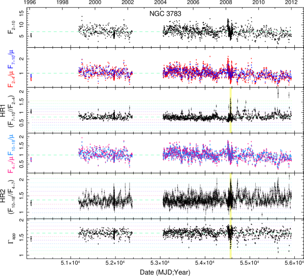
Figure A.1: Long-term continuum flux, hardness ratio, and $\Gamma_{\rm app}$ light curves for the Sy 1 NGC 3783. The top panel shows observed 2–10 keV flux, $F_{\rm 2-10}$, in units of $10^{-11}$ erg cm^-2 s^-1, with one point per observation. Error bars are frequently smaller than the data points. The second panel shows $F_{\rm 2-4}$ (red) and $F_{\rm 7-10}$ (blue), each normalized by their means. $HR1\equiv F_{\rm 7-10}/F_{\rm 2-4}$ is plotted in the third panel. The fourth panel shows $F_{\rm 4-7}$ (red) and $F_{\rm 10-18}$ (blue), each normalized by their means. $HR2\equiv F_{\rm 10-18}/F_{\rm 4-7}$ is plotted in the fifth panel. The bottom panel shows $\Gamma_{\rm app}$, the photon index obtained from fitting a simple power law plus $N_{\rm H,Gal}$ (ignoring all other components) to each observed spectrum. The colored dotted lines in panels 3, 5, and 6 indicate the 1–6$\sigma$ (standard deviation) levels. In all panels, the green dashed lines indicate the mean. The yellow shaded areas indicate the secure occultation event, shown in more detail in Fig. A.2.

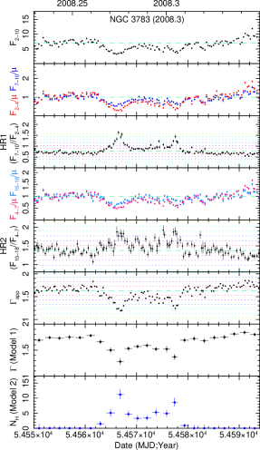
Figure A.2: Same as Fig. A.1, but zoomed in on the period of the secure occultation event at 2008.3. The bottom two panels show $\Gamma$ for Model 1 (wherein $N_{\rm H}$ is assumed to be zero) and $N_{\rm H}$ for Model 2, where $\Gamma$ is assumed to be frozen at 1.73. $N_{\rm H}$ is in units of $10^{22}$ cm^-2. Note the double-peaked behavior of $N_{\rm H}$($t$) for this event.

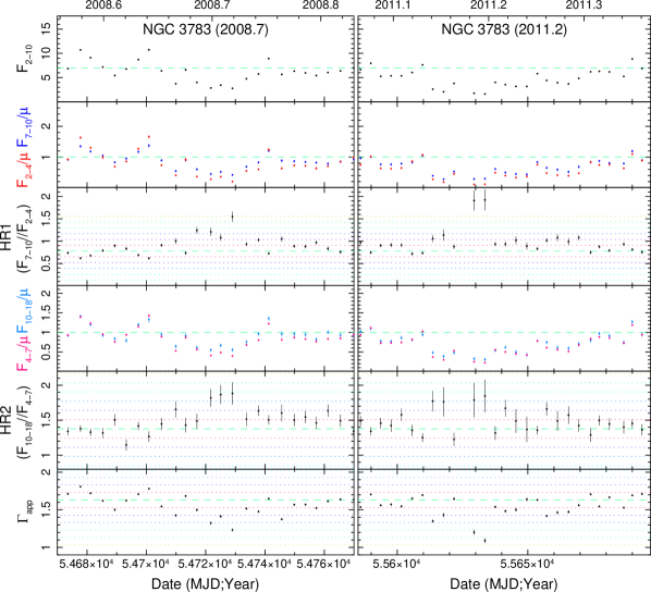
Figure A.3: Same as Fig. A.1, but zoomed in on two “candidate” events at 2008.7 and 2011.2.

A.2 Mkn 79 (Sy 1.2)

$\bullet$ 2003.5 (“Secure B”) and 2003.6 (“Secure B”): The long-term light curves are plotted in Fig. A.4. As seen there and in Fig. A.5, during MJD $\sim$ 52805–52818 (2003.5), $HR1$ increases to values ranging from 0.90 (just above $\langle HR1\rangle$) to 2.4, with large scatter. The average and peak values of $HR1$ during this period correspond to 2.8$\sigma$ and 5$\sigma$ deviation, respectively. $\langle\Gamma_{\rm app}\rangle$ during this time is 1.25, with a minimum value of 0.92 (3.2$\sigma$ deviation) at MJD 52816.0. The 10–18 keV continuum does not change as rapidly as the $<$7 keV continuum during this time; $HR2$ roughly doubled, to a $2\sigma$ deviation. No data were taken during MJD 50821–50839 due to a sun-angle gap. By MJD 52840, $HR1$ has returned to its mean value of 0.85.

During MJD $\sim$ 52861–52891 (2003.6), $HR1$ increases again, showing deviations as high as $3-6\sigma$, with an average deviation of 2.2$\sigma$ during this time. During this time, $\Gamma_{\rm app}$ reaches values as low as 1.0–1.1 (2.0–2.8$\sigma$), with large scatter; $\langle\Gamma_{\rm app}\rangle=1.39$.

We bin up data from MJD 52770–52925 into five bins of approximately 15–30 d as listed in Table 8. This yields only one time bin for each of the two candidate events (spectra 2 and 4), but smaller bin sizes would have yielded poor parameter constraints. We fit 3–23 keV data, keeping $R$ frozen at 0.7 (Rivers et al. 2013). We first test Model 1, with $N_{\rm H}$ frozen at 0, $\Gamma$ free, and $I_{\rm Fe}$ frozen at $5\times 10^{-5}$ ph cm^-2 s^-1. Best-fitting values are listed in Table 8; $\Gamma$ reaches values of 1.18$\pm$0.17 and 1.34$\pm$0.10 in spectra 2 and 4, respectively. We then add a neutral column of gas with zphabs for Model 2, keeping $\Gamma$ frozen at 1.78, the average from spectra 1, 3, and 5. $N_{\rm H}$ is $14.4^{+4.8}_{-4.2}$ and $11.5^{+3.2}_{-2.8}\times 10^{22}$ cm^-2 for spectra 2 and 4, respectively, with upper limits $\sim 2\times 10^{22}$ cm^-2 for spectra 1, 3, and 5. Best-fitting values of $\Gamma$ for Model 1 and $N_{\rm H}$ for Model 2 are plotted in Fig. A.5.

Values of $\chi^{2}_{\rm red}$ are virtually identical between Models 1 and 2, and span 0.46–0.81. That is, the observed spectral flattening could potentially be due to a combination of $\Gamma$ reaching extremely low values and spectral pivoting of the power law in or near the 10–18 keV band. However, adhering to our assumption that $\Gamma$ should not dip below 1.5, the occultation interpretation is then preferred in each of these cases.

We assign durations based on the $HR1$ light curve, but these durations are approximate due to large scatter in $HR1$. For the 2003.5 event, we observed ingress, but egress likely occurred during the monitoring gap; limits to the duration are 12.0–39.4 d. We cannot rule out that the possibility that the peak of the event occurred during the gap, in which case peak $N_{\rm H}$ might be higher than that observed. For the (complete) 2003.6 event, we estimate a duration of 34.5–37.9 d.

$\bullet$ 2009.9 (“Secure B”): At MJD$\sim 55155-55197$, some values of $HR1$ deviate as high as the 1–3$\sigma$ level, but $\langle HR1\rangle$ corresponds to the $\sim 1\sigma$ level. $F_{2-10}$ is about half the average value, but $F_{10-18}$ stays roughly constant, yielding an $HR2$ peak at the $\sim 2-2.5\sigma$ level albeit with large errors. We sum all spectra taken from MJD 55155 – 55197, plus all data in the $\sim$40 d periods before and after this period (spectra 6, 7, and 8 in Table 8). $I_{\rm Fe}$ is kept frozen at $4\times 10^{-5}$ ph cm^-2 s^-1. For spectrum #7, we apply Model 2 by freezing $\Gamma$ at 1.84, the average of $\Gamma$ from spectra 6 and 8; this yields $N_{\rm H}=7.6\pm 2.2\times 10^{22}$ cm^-2. We estimate a duration of $19.6-40.0$ d from the $HR1$ light curve.

$\bullet$ There are additional deviations in the long-term $HR1$ and/or $\Gamma_{\rm app}$ light curves which tend to catch the eye, but these deviations do not fulfill our selection criteria and are rejected:

At 2007.3, at MJD $54208-54219$, $HR1$ increases to $\sim$1.2, but these are only $\sim 1-2\sigma$ deviations. There are only a few points at $1\sigma$ deviation in the $HR2$ light curve as well; the 10–18 and 2–10 keV continua are both $\sim 40$ per cent below average during this period. $\langle\Gamma_{\rm app}\rangle$ during this period is 1.37, just under a 1$\sigma$ deviation, and with large scatter. Time-resolved spectroscopy to data summed between MJD $54208$ and $54219$, assuming that $\Gamma$ is frozen at 1.78, yields $N_{\rm H}<9.2\times 10^{22}$ cm^-2.

At 2008.2, MJD$\sim 54535-54590$, and several times near the end of 2008, MJD $\sim 54725-54830$, there are deviations in $HR1$ up to 2–5$\sigma$ levels, but with very large scatter and frequently large uncertainties. Roughly a third of the values of $\Gamma_{\rm app}$ during these times are $<$1.3, but there is very large scatter, and average values of $\Gamma_{\rm app}$ are at the $\sim 1\sigma$ level of deviation. Both the 10–18 and 2–10 keV continuua were $\sim 30-60$ per cent of their average values, and follow-up time-resolved spectroscopy cannot confirm significant increases in $N_{\rm H}$ (upper limits are in the range $3-5\times 10^{22}$ cm^-2).

Near 2009.1, at MJD $\sim 54856-54876$, a couple of $HR1$ points reach the 2$\sigma$ level, but errors are large, and $\langle HR1\rangle$ during this time is a $\ga 1\sigma$ deviation. All continuum flux light curves experience dips during this time to relatively low levels. Time-resolved spectroscopy cannot confirm any significant increase in $N_{\rm H}$.

Fig. A.7 shows a zoom-in on the 2008.0–2009.3 data with rejected events.

Table 8: Results of time-resolved spectral fits to Mkn 79, mid-2003 and late 2009

Start–stop	Expo	Model 1: $N_{\rm H}$ frozen at 0				Model 2: $N_{\rm H}$ free; $\Gamma$ frozen
(MJD)	(ks)	$\chi^{2}_{\rm red}$	$\Gamma$	$A_{1}$	$F_{2-10}$	$\chi^{2}_{\rm red}$	$N_{\rm H}$ ($10^{22}$ cm-2)	$A_{1}$	$F_{2-10}$
52770.2–52804.3 (#1)	14.8	0.67	$1.73\pm 0.06$	$4.7\pm 0.5$	1.98	0.70	$<$2.0	$5.1\pm 0.1$	1.97
52806.2–52818.2 (#2)	3.4	0.50	$1.18\pm 0.17$	$1.2\pm 0.3$	1.22	0.50	$14.4^{+4.8}_{-4.2}$	$4.9^{+0.6}_{-0.5}$	1.14
52843.7–52858.3 (#3)	4.7	0.64	$1.87\pm 0.11$	$6.0\pm 1.2$	1.89	0.69	$<$1.4	$5.1\pm 0.2$	1.85
52861.0–52891.3 (#4)	9.7	0.73	$1.34\pm 0.10$	$1.7\pm 0.3$	1.26	0.80	$11.5^{+3.2}_{-2.8}$	$4.7\pm 0.3$	1.18
52895.8–52925.6 (#5)	11.6	0.72	$1.75\pm 0.07$	$4.6\pm 0.7$	1.81	0.74	$<$2.1	$5.0^{+0.2}_{-0.1}$	1.80
55115.8–55153.8 (#6)	14.6	0.92	$1.83\pm 0.04$	$6.5\pm 0.7$	2.12	0.94	$<1.1$	$6.4\pm 0.1$	2.08
55155.8–55195.1 (#7)	18.6	0.79	$1.44\pm 0.08$	$1.8\pm 0.3$	1.17	1.15	$7.6\pm 2.2$	$4.4\pm 0.3$	1.17
55197.9–55235.7 (#8)	18.0	0.69	$1.84\pm 0.05$	$6.2\pm 0.4$	1.99	0.94	$<1.0$	$5.9\pm 0.1$	1.94

$A_{1}$ is the 1 keV normalization of the power law in units of $10^{-3}$ ph cm^-2 s^-1 keV^-1. $F_{2-10}$ is the observed/absorbed model flux in units of $10^{-11}$ erg cm^-2 s^-1. $I_{\rm Fe}$ is kept frozen at 5 and $4\times 10^{-5}$ ph cm^-2 s^-1 for the 2003 and 2009 spectra, respectively. For Model 2, $\Gamma$ is frozen at 1.78 and 1.84 for the 2003 and 2009 spectra, respectively. Each spectral fit is performed over the 3–23 keV bandpass and has 45 $dof$.

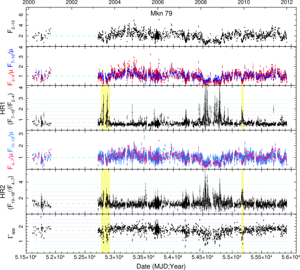
Figure A.4: Same as Fig. A.1, but for the Sy 1.2 Mkn 79. The yellow shaded areas in mid 2003 and in late 2009 indicate “secure” eclipse events; see Figs. A.5 and A.6 for zoom-ins on these periods.

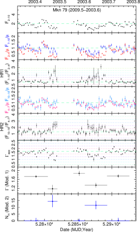
Figure A.5: Same as Fig. A.4, but a zoom-in on two “secure B” occultation events in mid-2003. The bottom two panels show $\Gamma$ from Model 1 ($N_{\rm H}$ set to 0) and $N_{\rm H}$ in units of $10^{22}$ cm^-2 from Model 2 ($\Gamma$ frozen at 1.78).

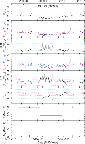
Figure A.6: Same as Fig. A.4, but a zoom-in on the “secure B” occultation event in late 2009. The bottom two panels show $\Gamma$ from Model 1 ($N_{\rm H}$ set to 0) and $N_{\rm H}$ in units of $10^{22}$ cm^-2 from Model 2 ($\Gamma$ frozen at 1.84).

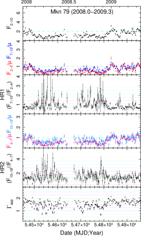
Figure A.7: Same as Fig. A.4, but a zoom-in on four rejected events in 2008 and early 2009.

A.3 Mkn 509 (Sy 1.2)

The long-term light curves are plotted in Fig. A.8, with a zoom-in on late 2005 plotted in Fig. A.9.

2005.9 (“Secure B”): The $HR1$ light curve in Fig. A.9 shows an upturn from the baseline value of $\sim$0.6 to 1.2 over a 30 d period in late 2009, with a $\sim 5\sigma$ peak deviation by MJD 53736, after which monitoring was interrupted for 59 d due to sun-angle constraints. $\Gamma_{\rm app}$ drops from about 1.7 to 1.3 during this time, a $\sim 4\sigma$ deviation.

During this time, RXTE monitored the source once every 3 d. For time-resolved spectroscopy, we grouped the individual spectra into bins of 15 d each. We fit the 3–23 keV spectra keeping $R$ and $I_{\rm Fe}$ frozen at their respective time-averaged values of 0.15 and $7\times 10^{-5}$ ph cm^-2 s^-1; results are listed in Table 9. With Model 1, acceptable fits ($\chi^{2}_{\rm red}$ = 0.52–0.68) are obtained, although $\Gamma$ flattens to the very low value of $1.37\pm 0.06$ during spectrum #6. We then test Model 2, freezing $\Gamma$ to 1.72, the average of the values in spectra #1–3 and #7, and close to the time-averaged value found by Rivers et al. (2011), 1.75. Acceptable fits spanning a nearly identical range of $\chi^{2}_{\rm red}$ are obtained, with $N_{\rm H}$ peaking at $8.8\pm 1.7\times 10^{22}$ cm^-2 during spectrum #6, and with upper limits during spectra #1–3 and 7. Best-fitting values of $\Gamma$ for Model 1 and $N_{\rm H}$ for Model 2 are plotted in Fig. A.9.

Under the assumption that an eclipse occurred, it is difficult to pin down the exact duration because the event ended sometime during the 60 d sun-angle gap, between MJD 53736 and 53795; peak $N_{\rm H}$ could thus be higher than that measured during spectrum $\#6$, $8.8\pm 1.7\times 10^{22}$ cm^-2. From the $HR1$ light curve, we assign a duration of 26–94 d. If the occulting cloud is symmetric in density along the transverse direction, then the total duration can be $\sim 55-90$ d, with peak $N_{\rm H}$ occurring immediately before the sun-angle gap in the former case (i.e., during the times constrained by spectrum $\#5$), or with peak $N_{\rm H}$ slightly higher and occurring $\sim$15 d into the gap in the latter case.

Table 9: Results of time-resolved spectral fits to Mkn 509, 2005.9

Start–stop	Expo	Model 1: $N_{\rm H}$ frozen at 0				Model 2: $N_{\rm H}$ free; $\Gamma$ frozen at 1.72
(MJD)	(ks)	$\chi^{2}_{\rm red}$	$\Gamma$	$A_{1}$	$F_{2-10}$	$\chi^{2}_{\rm red}$	$N_{\rm H}$ ($10^{22}$ cm-2)	$A_{1}$	$F_{2-10}$
53650.31–53662.56 ($\#1$)	6.4	0.67	$1.74^{+0.04}_{-0.05}$	$11.7\pm 1.0$	4.32	0.68	$<0.5$	$11.4\pm 0.2$	4.31
53665.18–53677.10 ($\#2$)	8.0	0.63	$1.72\pm 0.04$	$11.1\pm 0.9$	4.22	0.63	$<0.8$	$11.1\pm 0.2$	4.22
53680.11–53692.37 ($\#3$)	9.7	0.52	$1.71^{+0.04}_{-0.03}$	$11.8^{+0.9}_{-0.7}$	4.55	0.53	$<0.8$	$12.0^{+0.2}_{-0.1}$	4.55
53695.25–53707.58 ($\#4$)	8.3	0.54	$1.65^{+0.04}_{-0.05}$	$8.6\pm 0.7$	3.68	0.61	$1.1\pm 0.8$	$10.0^{+0.4}_{-0.3}$	3.64
53710.46–53722.19 ($\#5$)	8.2	0.53	$1.52^{+0.04}_{-0.05}$	$6.5^{+0.6}_{-0.5}$	3.45	0.73	$4.5\pm 1.2$	$10.4\pm 0.3$	3.33
53725.91–53736.34 ($\#6$)	7.8	0.67	$1.37\pm 0.06$	$3.7\pm 0.4$	2.51	0.80	$8.8\pm 1.7$	$8.4^{+0.4}_{-0.3}$	2.37
53795.10–53806.97 ($\#7$)	7.9	0.68	$1.70\pm 0.06$	$11.5^{+1.0}_{-0.8}$	4.56	0.65	$<0.9$	$12.1\pm 0.2$	4.58

$A_{1}$ is the 1 keV normalization of the power law in units of $10^{-3}$ ph cm^-2 s^-1 keV^-1. $F_{2-10}$ is the observed/absorbed model flux in units of $10^{-11}$ erg cm^-2 s^-1. $I_{\rm Fe}$ is kept frozen at $7\times 10^{-5}$ ph cm^-2 s^-1. Each spectral fit is performed over the 3–23 keV bandpass and has 45 $dof$.

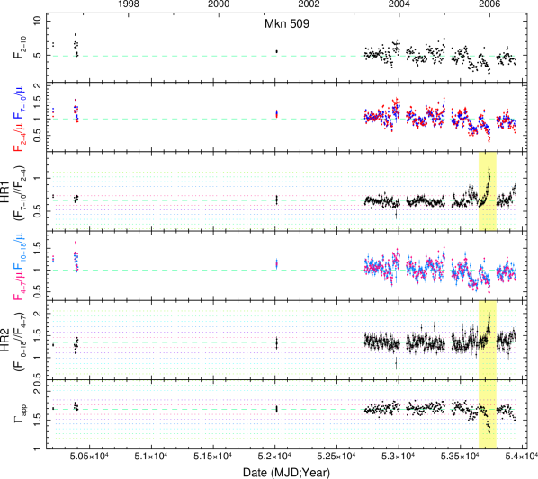
Figure A.8: Same as Fig. A.1, but for the Sy 1.2 Mkn 509. The yellow shaded area in late 2005 indicates a candidate eclipse event; see Fig. A.9 for a zoom-in on this period.

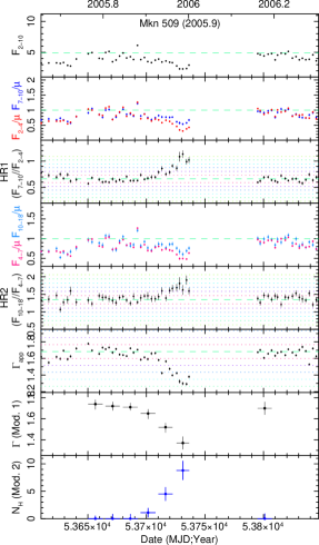
Figure A.9: Same as Fig. A.8, but a zoom-in on the candidate occultation event in late 2005. The bottom two panels show $\Gamma$ from Model 1 ($N_{\rm H}$ set to 0) and $N_{\rm H}$ in units of $10^{22}$ cm^-2 from Model 2 ($\Gamma$ frozen at 1.72).

A.4 MR 2251–178 (Sy 1.5/QSO)

$\bullet$ 1996 (“Secure A”) This source was observed by RXTE for 3 d in 1996 MJD 50426-9, then subjected to sustained monitoring during 2004 March – 2011 December, as seen in Fig. A.10. Values of $HR1$ in 1996 are $\sim 1.0-1.1$, a $\sim 4\sigma$ deviation from the mean value of 0.68 from the 2004–2011 data. $\Gamma_{\rm app}$ during 1996 is 1.5, a $\sim 2-3\sigma$ deviation.

The X-ray spectrum of this source is characterized by absorption from gas spanning a wide range of ionization states; Gofford et al. (2011) quantify five such zones using combined Suzaku + Swift-Burst Alert Telescope spectra. Furthermore, there is evidence for the column densities of at least some of these zones to vary over timescales of months–years (Kaspi et al. 2004). RXTE is not strongly sensitive to the effect of the highest ionization zones of absorption, log($\xi$) $\ga 3$, e.g., ”Zones 3–5” in Gofford et al. (2011). Any absorbing column we detect in excess of $N_{\rm Gal}$ may potentially be analogous to (or even potentially identified as) an overdense region of ”Zone 1” from Gofford et al. (2011; with log($\xi$) $\sim-0.23$ and $N_{\rm H}\sim 5\times 10^{20}$ cm^-2), or the absorber with log($\xi$) $\sim+0.02$ and $N_{\rm H}\sim 2.4\times 10^{21}$ cm^-2 measured by Gibson et al. (2005) using a 2002 Chandra-High-Energy Transmission Grating Spectrometer (HETGS) observation. Here, we fit the RXTE spectra assuming full-covering neutral absorption only.

We sum all the data during the 1996 campaign; the good exposure for the PCA was 90.1 ks. The good exposure time per High-Energy X-ray Timing Experiment (HEXTE) cluster is 20.1/20.5 ks for A/B, with the source detected only out to 25 keV, so we use PCA data only. We fit 3–23 keV data, and assume no reflection component and no high-energy rollover (see Rivers et al. 2011a). We first apply Model 1, keeping the Fe K$\alpha$ line energy and width $\sigma$ frozen at 6.0 keV and 0.9 keV, respectively. This fit yields $\Gamma=1.52\pm 0.01$, but $\chi^{2}/dof$ is 175.2/42 = 4.2, with poor data/model residuals showing strong curvature up to the $\pm$6 per cent level below 10 keV. We apply Model 2, keeping $\Gamma$ free, and obtain a fit with $\chi^{2}/dof$ = 95.8/41 and data/model residuals $\la 2$ per cent, consistent with PCA calibration. Best-fitting model parameters are $N_{\rm H}=6.6^{+0.8}_{-1.4}\times 10^{22}$ cm^-2, $\Gamma=1.73^{+0.02}_{-0.06}$, and $I_{\rm Fe}$ fell to $3.1\pm 1.3\times 10^{-5}$ ph cm^-2 s^-2.

Fig. A.11 shows a zoom-in on the 1996 data; we find no evidence then for strong variations in $HR1$ on timescales $<$3 d. Constraints on the duration of the event from RXTE data alone are poor; we can only set a lower limit of 3 d, the length of the 1996 campaign. Peak $N_{\rm H}$ may of course be higher than that observed in 1996. Dadina (2007), fitting two BeppoSAX observations in 1998 June and 1998 November, noted total columns consistent with $\sim 1-2\times$$N_{\rm H,Gal}$. In the context of an absorption event, this measurement suggests that the event had ended by 1998 June. Reeves & Turner (2000), fitting ASCA spectra obtained in 1993 November–December, found $N_{\rm H}<1\times 10^{20}$ cm^-2, implying an upper limit for the duration of the event of $\sim 4.5$ yr.

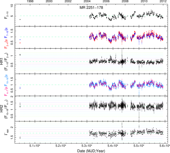
Figure A.10: Same as Fig. A.1, but for the Sy 1.5/QSO MR 2251–178.

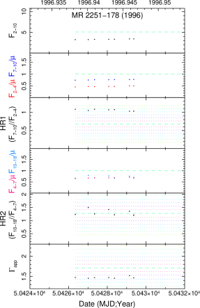
Figure A.11: Same as Fig. A.10, but a zoom-in on the 1996 data.

A.5 NGC 3227 (Sy 1.5)

The long-term light curves are plotted in Fig. A.12.

$\bullet$ 2000.9–2001.2 (“Secure A”): Lamer et al. (2003) confirmed a complete eclipse event (ingress and egress) by a full-covering cloud. They determined the cloud to be mildly ionized via a contemporaneous XMM-Newton observation, with log($\xi$, erg cm s^-1) $\sim-0.3-0$. Our $HR1$, $HR2$, and $\Gamma_{\rm app}$ light curves show peak deviations up to the $\ga 6-8$, $\ga 3-5$, and the $\sim 4$$\sigma$ levels, respectively, and $\Gamma_{\rm app}$ gets as low as $\sim 0.5$. We refer the reader to Lamer et al. (2003) for details of time-resolved spectral fitting and fitting the $N_{\rm H}$($t$) profile. Lamer et al. (2003) found values of peak $N_{\rm H}$ of $19$ and $26\times 10^{22}$ cm^-2 based on fits to the $N_{\rm H}$($t$) profile using a uniform-density sphere and a $\beta$-profile fits, respectively; we adopt the latter value for the rest of this paper. Based on our $HR1$ light curve, we adopt a duration of 77–94 d, similar to values used by Lamer et al. (2003).

$\bullet$ 2002.8 (“Secure B”): As seen in Fig. A.13, two consecutive points at MJD 52565.7 and 52567.8 show anomalously high $HR1$ values: $2.54\pm 0.15$ (2.9$\sigma$) and $1.92\pm 0.10$ (1.8$\sigma$), respectively. $\Gamma_{\rm app}=1.01\pm 0.02$ and $1.12\pm 0.02$, $\sim 2\sigma$ deviations. $HR2$ shows only $\sim 1.5\sigma$ deviations.

We sum spectra obtained during MJD 52541–52581 in groups of two to match the time resolution of the putative event, and fit each 3–23 keV spectrum, keeping $I_{\rm Fe}$ frozen at $6\times 10^{-5}$ ph cm^-2 s^-1. Fitting spectrum #7 with Model 1 yields a fit with $\chi^{2}_{\rm red}=1.34$ and with strong systematic curvature in the data/model residuals $\sim 3-7$ keV; $\Gamma$ is $1.13\pm 0.08$. Applying Model 1 to the other spectra yields an average value of $\Gamma$ of 1.61. Applying Model 2 to spectrum #7 with $\Gamma$ frozen at 1.61 fixed data/model residuals; $\chi^{2}_{\rm red}=0.55$, and $N_{\rm H}=13.3^{+2.6}_{-2.2}\times 10^{22}$ cm^-2. Results for all spectra are listed in Table 10. From the start/stop times of the two observations, limits on the duration of the event are 2.1–6.6 d.

Using XMM-Newton, Markowitz et al. (2009) modeled two outflowing zones of ionized absorption, both with $N_{\rm H}\sim 1-2\times 10^{21}$ cm^-2, and with log($\xi$) $\sim 1.2-1.4$ and $\sim$2.9. Neither are expected to significantly impact the time-resolved PCA spectra. Due to the much higher column and lower ionization, it is likely that the eclipse events detected with RXTE are likely distinct from these outflowing warm absorbers.

$\bullet$ Additional events do not meet our selection criteria and are rejected due to being single points only (failing criterion 2). As seen in Fig. A.14, a single point at MJD 53207 (2004 Jul 21) shows a very strong $HR1$ deviation up to $3.0\pm 0.29$, a $3.7\sigma$ deviation. $\Gamma_{\rm app}=0.80\pm 0.03$, a 3.2$\sigma$ deviation; $HR2$ shows a $2\sigma$ deviation.

At 2000.3, $HR1$ goes to a 6$\sigma$ deviation. There are four single points in the period 2000.3–2000.4 where $HR2$ goes to a $\geq$2$\sigma$ deviation, but with extremely large errors. Again, however, each of these events fails criterion 2 and is rejected.

The bottom two panels in Fig. A.13 also suggest a significant increase in $N_{\rm H}$ for spectrum #4, at MJD 52555. Given the fact that the continuum flux was relatively low in all wavebands, the near-identical values of $\chi^{2}_{\rm red}$ between Models 1 and 2, and especially the fact that only 1 point shows a $>$1$\sigma$ deviation in both the $HR1$ and $\Gamma_{\rm app}$ light curves (thus failing criterion 2), we do not consider this as an event.

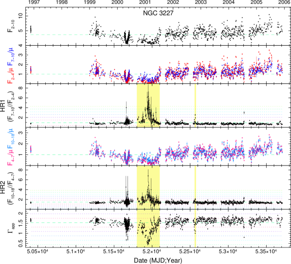
Figure A.12: Same as Fig. A.1, but for the Sy 1.5 NGC 3227. The yellow shaded areas indicate putative eclipse events. The reader is referred to Lamer et al. (2003) for details on the 2000–2001 event. A zoom-in on late 2002 is shown in Fig. A.13.

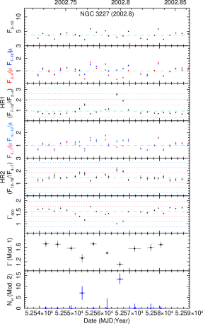
Figure A.13: Same as Fig. A.12, but a zoom-in on the “secure B” occultation event in late 2002. The bottom two panels show $\Gamma$ from Model 1 ($N_{\rm H}$ set to 0) and $N_{\rm H}$ in units of $10^{22}$ cm^-2 from Model 2 ($\Gamma$ frozen at 1.61).

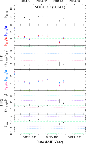
Figure A.14: Same as Fig. A.12, but a zoom-in on the rejected event in 2004.

Table 10: Results of time-resolved spectral fits to NGC 3227, late 2002

Start–stop	Expo	Model 1: $N_{\rm H}$ frozen at 0				Model 2: $N_{\rm H}$ free; $\Gamma$ frozen
(MJD)	(ks)	$\chi^{2}_{\rm red}$	$\Gamma$	$A_{1}$	$F_{2-10}$	$\chi^{2}_{\rm red}$	$N_{\rm H}$ ($10^{22}$ cm-2)	$A_{1}$	$F_{2-10}$
52541.11–52543.16 (#1)	1.7	0.58	$1.69\pm 0.08$	$9.7^{+1.5}_{-1.3}$	4.12	0.66	$<0.7$	$8.3\pm 0.3$	4.06
52544.99–52547.03 (#2)	1.9	0.57	$1.68\pm 0.09$	$7.9\pm 1.3$	3.38	0.62	$<0.7$	$6.8\pm 0.3$	3.34
52549.13–52551.92 (#3)	2.0	0.62	$1.57\pm 0.07$	$8.4\pm 1.3$	4.33	0.64	$<1.4$	$9.1\pm 0.3$	4.36
52553.36–52555.07 (#4)	1.6	0.70	$1.30\pm 0.11$	$3.3\pm 0.7$	2.72	0.60	$7\pm 3$	$7.1\pm 0.6$	2.56
52556.96–52558.98 (#5)	1.9	0.33	$1.69\pm 0.06$	$12.9^{+1.6}_{-1.4}$	5.42	0.46	$<0.5$	$11.1\pm 0.3$	5.34
52561.97–52563.04 (#6)	1.7	1.03	$1.44\pm 0.04$	$6.7^{+1.0}_{-0.9}$	4.23	0.72	$<4.5$	$10.0\pm 0.5$	4.00
52565.74–52567.87 (#7)	1.8	1.34	$1.13\pm 0.08$	$3.0^{+0.5}_{-0.4}$	3.18	0.55	$13.3^{+2.6}_{-2.2}$	$9.9\pm 0.6$	2.97
52569.63–52573.72 (#8)	1.8	1.03	$1.56\pm 0.08$	$7.4\pm 1.1$	3.85	0.95	$<2.0$	$8.4\pm 0.5$	3.71
52575.90–52578.28 (#9)	1.9	0.79	$1.59\pm 0.10$	$6.2^{+1.2}_{-1.0}$	3.10	0.80	$<2.0$	$6.4\pm 0.3$	3.11
52579.57–52581.31 (#10)	1.7	0.95	$1.67\pm 0.08$	$9.7^{+1.5}_{-1.3}$	4.23	0.98	$<0.8$	$8.6\pm 0.3$	4.19

$A_{1}$ is the 1 keV normalization of the power law in units of $10^{-3}$ ph cm^-2 s^-1 keV^-1. $F_{2-10}$ is the observed/absorbed model flux in units of $10^{-11}$ erg cm^-2 s^-1. $I_{\rm Fe}$ is kept frozen $6\times 10^{-5}$ ph cm^-2 s^-1. For Model 2, $\Gamma$ is frozen at 1.61. Each spectral fit is performed over the 3–23 keV bandpass and has 45 $dof$.

A.6 Cen A (NLRG)

$\bullet$ 2010–2011 (“Secure A”): Our $HR1$, $HR2$, and $\Gamma_{\rm app}$ light curves (Fig. A.15) each suggest strong spectral flattening (at roughly 3–4$\sigma$ deviation) over a $\sim$6 month period in 2010–2011 (MJD $\sim$ 55430–55620), during a period of monitoring once every 2 d. The means and standard deviations of $HR1$, $HR2$, and $\Gamma_{\rm app}$ in Fig. A.15 were calculated omitting data during this period to avoid biases due to the large number of individual points during the eclipse. A zoom-in on this time period is shown in Fig. A.16. Time-resolved spectroscopy by Rivers et al. (2011b) successfully deconvolved $\Gamma$ and $N_{\rm H}$ and confirmed a complete eclipse (ingress and egress) with peak $\Delta$$N_{\rm H}$ of $8\times 10^{22}$ cm^-2 above the “baseline” level of $\sim 20\times 10^{22}$ cm^-2; the reader is referred to that paper for details. With spectra binned to once every 10 d and an event duration of a little over 170 d, this event is likely the best-observed eclipse so far in terms of resolving the $N_{\rm H}$ profile.

The profile is consistent with a cloud whose density was symmetric along the direction of transit (as opposed to a “comet-shaped” cloud, e.g., Maiolino et al. 2010); to the eye the $HR1$ and $HR2$ light curves may look slightly skewed, but fits to the $N_{\rm H}$ profile were consistent with a symmetric cloud. A centrally-concentrated sphere with a linear density profile was a better fit than a constant-density sphere. From our $HR1$ light curve, we adopt a duration of 170.2–184.5 d.

$\bullet$ 2003–2004 (“Secure A”): Similar changes in $HR1$ and $\Gamma_{\rm app}$ suggest an event with roughly similar $\Delta$$N_{\rm H}$ peaking in 2003–2004. However, constraints on the duration of the event and peak $N_{\rm H}$ are poor because RXTE observed Cen A during this time via three clusters of observations separated by months–years, as opposed to via sustained monitoring. Spectral fits by Rothschild et al. (2011; see their fig. 4) reveal $N_{\rm H}=23\times 10^{22}$ cm^-2 during the 2003 March campaign and $24-26\times 10^{22}$ cm^-2 during 2004 January and February, compared to $15-18\times 10^{22}$ cm^-2 measured during the 2000 January and earlier campaigns and the 2005 August and later campaigns. The spectral fits of Rothschild et al. (2011) thus indicate an observed $\Delta$$N_{\rm H}$ = $8\pm 1\times 10^{22}$ cm^-2 with a similar baseline $N_{\rm H}$ as the 2010–2011 event. Constraints on the duration of the event from the $HR1$ light curve are 356–2036 d.

We also present evidence that the “baseline” level of $N_{\rm H}$ is not constant. There is a small “dip” in the $HR1$ light curve in 2010, shortly after the 2-d monitoring commenced. We sum up individual spectra from the first four months of monitoring in groups of three (6 d; Rivers et al. 2011b binned every five spectra / 10 d). We leave $\Gamma$ free, but hold $I_{\rm Fe}$ frozen at $4.2\times 10^{-4}$ ph cm^-2 s^-1. The resulting values of $\Gamma$($t$) and $N_{\rm H}$($t$) are displayed in Fig. A.17 and listed in Table 11. The value of $N_{\rm H}$($t$) reaches a maximum in bin #2 (covering MJD 55226.7–55232.3), with $N_{\rm H}=21.7\pm 0.9\times 10^{22}$ cm^-2, reaches a minimum in bin #8 (MJD 55264.5–55270.4) with $N_{\rm H}=18.6^{+0.9}_{-0.8}\times 10^{22}$ cm^-2, and returns to a maximum value of $21.9\pm 0.7\times 10^{22}$ cm^-2 in bin #21 (MJD 55341.1–55350.5). As the uncertainties on each $N_{\rm H}$ point are 90 per cent confidence, this difference is a $\sim 2.2\sigma$ result. This result cannot be due to degeneracy between $\Gamma$ and $N_{\rm H}$: an increase in $\Gamma$ is expected to be associated with an increase in $N_{\rm H}$, contrary to what is observed. However, freezing $\Gamma$ at the average value of 1.85 does not significantly change the $N_{\rm H}$($t$) light curve; those values are plotted in gray in Fig. A.17. Summing over all spectra, the total value of $\chi^{2}$/$dof$ is 1067.95/1113, compared to 1037.92/1092 with $\Gamma$ free; this means that allowing $\Gamma$ to be free improves the fits only at 93.3 per cent confidence according to an $F$-test.

Table 11: Time-resolved spectral fits to Cen A, early 2010

Start–stop	Expo		$N_{\rm H}$		$A_{1}$
(MJD)	(ks)	$\chi^{2}_{\rm red}$	($10^{22}$ cm-2)	$\Gamma$	(ph cm-2 s-1 keV-1)	$F_{2-10}$
55221.53–55225.65 (#1)	2.4	0.88	$21.7\pm 0.9$	1.82$\pm$0.03	$0.214^{+0.016}_{-0.014}$	34.62
55227.83–55231.27 (#2)	2.4	0.97	$21.8\pm 0.9$	1.81$\pm$0.03	$0.214^{+0.016}_{-0.014}$	35.13
55233.29–55237.65 (#3)	2.8	1.08	$21.3\pm 0.8$	1.85$\pm$0.03	$0.243^{+0.016}_{-0.014}$	37.66
55239.84–55243.70 (#4)	2.2	1.02	$21.2\pm 0.9$	1.88$\pm$0.03	$0.254^{+0.020}_{-0.017}$	37.43
55247.62–55251.64 (#5)	3.3	0.97	$18.8^{+0.7}_{-0.6}$	1.85$\pm$0.02	$0.244^{+0.014}_{-0.012}$	39.85
55253.90–55257.92 (#6)	2.5	0.84	$19.2\pm 0.9$	1.87$\pm$0.03	$0.187^{+0.016}_{-0.014}$	29.29
55259.59–55263.45 (#7)	2.6	0.70	$20.5^{+1.0}_{-0.9}$	1.88$\pm$0.03	$0.191^{+0.016}_{-0.014}$	28.64
55265.56–55269.48 (#8)	2.6	0.97	$18.6^{+0.9}_{-0.8}$	1.82$\pm$0.03	$0.190^{+0.014}_{-0.013}$	32.66
55271.35–55275.12 (#9)	2.4	0.93	$18.9^{+0.9}_{-0.8}$	1.86$\pm$0.03	$0.217^{+0.016}_{-0.014}$	35.00
55277.71–55281.56 (#10)	2.4	0.75	$19.4^{+0.9}_{-0.8}$	1.88$\pm$0.03	$0.220^{+0.017}_{-0.015}$	33.54
55283.86–55287.54 (#11)	2.2	0.76	$18.9^{+0.9}_{-0.8}$	1.84$\pm$0.03	$0.209^{+0.016}_{-0.014}$	34.64
55289.33–55293.49 (#12)	2.8	1.08	$19.3^{+0.8}_{-0.7}$	$1.83^{+0.03}_{-0.02}$	$0.221^{+0.014}_{-0.013}$	37.10
55295.29–55299.64 (#13)	2.8	1.42	$19.2^{+0.9}_{-0.8}$	1.83$\pm$0.03	$0.184^{+0.014}_{-0.012}$	31.11
55303.40–55306.94 (#14)	2.5	1.03	$20.0\pm 0.9$	1.84$\pm$0.03	$0.191^{+0.015}_{-0.013}$	30.76
55309.87–55313.43 (#15)	2.6	0.66	$19.5\pm 0.8$	1.83$\pm$0.03	$0.219^{+0.015}_{-0.013}$	36.18
55315.44–55319.17 (#16)	3.1	1.18	$20.4\pm 0.7$	1.84$\pm$0.02	$0.271^{+0.015}_{-0.013}$	42.99
55321.25–55325.45 (#17)	2.9	0.59	$19.9\pm 0.8$	1.84$\pm$0.02	$0.225^{+0.015}_{-0.013}$	36.36
55327.28–55331.54 (#18)	2.5	0.95	$21.0^{+0.9}_{-0.8}$	1.82$\pm$0.03	$0.217^{+0.015}_{-0.014}$	35.43
55333.61–55338.38 (#19)	2.4	1.03	$21.3\pm 0.8$	$1.84^{+0.03}_{-0.02}$	$0.272^{+0.018}_{-0.016}$	42.31
55339.42–55342.86 (#20)	2.1	1.24	$20.9^{+0.9}_{-0.8}$	1.85$\pm$0.03	$0.250^{+0.018}_{-0.016}$	39.02
55345.33–55349.51 (#21)	2.6	0.91	$21.9\pm 0.7$	1.88$\pm$0.02	$0.303^{+0.019}_{-0.017}$	43.94

Results of time-resolved spectroscopy for Cen A to quantify the small ”dip” in the baseline level of $N_{\rm H}$ in early 2010 (approx. MJD 55230–55330). $A_{1}$ is the 1 keV normalization of the power law. $F_{2-10}$ is the observed/absorbed model flux in units of $10^{-11}$ erg cm^-2 s^-1. $I_{\rm Fe}$ is frozen at $4.2\times 10^{-4}$ ph cm^-2 s^-1. Each spectral fit is performed using the 3–30 keV bandpass and has 52 $dof$.

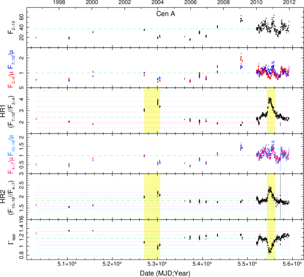
Figure A.15: Same as Fig. A.1, but for the NLRG Cen A. The yellow shaded areas indicate eclipse events whose spectroscopic analyses can be found in by Rivers et al. (2011b) and Rothschild et al. (2011).

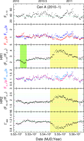
Figure A.16: A zoom-in on the 2010–2011 occultation event in Cen A; see Rivers et al. (2011b) for details of fits to the time-resolved spectra and to the resulting $N_{\rm H}$($t$) profile. The green shaded area denotes a dip in $HR1$ and thus $N_{\rm H}$; see Fig. A.17.

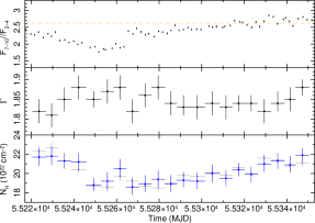
Figure A.17: Time-resolved spectral fits for the first four months of monitoring of Cen A in 2010, with a moderately higher time resolution compared to Rivers et al. (2011b). The resulting $\Gamma$($t$) and $N_{\rm H}$($t$) light curves are depicted in the middle and bottom panels, respectively. In the bottom panel, the blue and gray points denote $N_{\rm H}$($t$) with $\Gamma$ free and with $\Gamma$ frozen at 1.85, respectively.

A.7 NGC 5506 (Sy 1.9)

$\bullet$ 2000.2 (“Secure A”): The long-term light curves are plotted in Fig. A.18. During a period of intensive monitoring in early 2000 (Fig. A.19, with four observations per day, two consecutive observations (at MJD 51624.9 and 51625.1) show anomalous increases in $HR1$ from its mean value of 0.88 with a standard deviation of 0.10 to values of 1.41$\pm$0.02 and 1.48$\pm$0.02, deviations of 5.2 and 6.0$\sigma$. $\Gamma_{\rm app}$ drops from 1.6 to 1.3 ($>4\sigma$ deviation).

We perform time-resolved spectroscopy by summing spectra together in groups of two. We fit 3–23 keV data, allowing $N_{\rm,H}$, $\Gamma$, $A_{1}$ and $I_{\rm Fe}$ to vary from their best-fitting time-averaged values. Uncertainties on $I_{\rm Fe}$ within each time bin are usually over 50 per cent, and so we re-fit with $I_{\rm Fe}$ held at $2.5\times 10^{-4}$ ph cm^-2 s^-1. The results are listed in Table 12. The resulting best-fitting parameters for $\Gamma$ and $N_{\rm H}$ are plotted in Fig. A.19.

$N_{\rm H}$ increases from an average of $5.4\pm 1.0\times 10^{22}$ to $9.4\pm 1.1\times 10^{22}$ cm^-2 during MJD 51624.9–51625.1. For the MJD 51624.9–51625.1 spectrum, freezing $\Gamma$ to 1.93 causes $\chi^{2}_{\rm red}$ to increase from 1.08 to 1.19; $N_{\rm H}$ goes to a value of $10.7\pm 0.6\times 10^{22}$ cm^-2 (consistent with the value obtained with $\Gamma$ free), but there are systematic data/model residuals around 5 keV, at the $\sim 8$ per cent level.

We conclude that a short-duration obscuration event with $\Delta$$N_{\rm H}=4.0\pm 1.4\times 10^{22}$ cm^-2 occurred. Given the start and stop times of these observations and the surrounding ones, the duration of the event must be in the range $17.2-69.0$ ks.

Table 12: Time-resolved spectral fits to NGC 5506, 2000.2

Start–stop	Expo		$N_{\rm H}$		$A_{1}$
(MJD)	(ks)	$\chi^{2}_{\rm red}$	($10^{22}$ cm-2)	$\Gamma$	($10^{-2}$ ph cm-2 s-1 keV-1)	$F_{2-10}$
51623.47–51623.68 ($\#1$)	1.7	0.61	$4.6\pm 1.1$	$1.98^{+0.06}_{-0.05}$	$4.1^{+0.6}_{-0.5}$	9.53
51623.86–51624.14 ($\#2$)	1.6	0.71	$6.2^{+1.2}_{-1.1}$	$2.06^{+0.06}_{-0.05}$	$5.1^{+0.7}_{-0.6}$	9.91
51624.47–51624.67 ($\#3$)	2.3	0.66	$5.0\pm 0.9$	$2.06\pm 0.05$	$5.3^{+0.6}_{-0.5}$	10.73
51624.94–51625.14 ($\#4$)	2.0	1.08	$9.4\pm 1.1$	$1.86^{+0.05}_{-0.04}$	$4.0^{+0.5}_{-0.4}$	9.53
		1.19	$10.7\pm 0.6$	1.93 (frozen)	$4.7\pm 0.1$	9.45
51625.47–51625.67 ($\#5$)	2.3	0.79	$4.9\pm 1.2$	$2.01\pm 0.06$	$3.7^{+0.5}_{-0.4}$	8.09
51625.94–51626.14 ($\#6$)	2.0	0.71	$5.1\pm 1.1$	$2.02^{+0.06}_{-0.05}$	$4.2\pm 0.6$	8.84
51626.47–51626.67 ($\#7$)	2.3	0.91	$6.5\pm 0.9$	$2.08^{+0.05}_{-0.04}$	$5.9\pm 0.6$	10.73

Results of time-resolved spectroscopy for NGC 5506 in early 2000. $A_{1}$ is the 1 keV normalization of the power law. $F_{2-10}$ is the observed/absorbed model flux in units of $10^{-11}$ erg cm^-2 s^-1. $I_{\rm Fe}$ is frozen at $2.5\times 10^{-4}$ ph cm^-2 s^-1. Each spectral fit is performed over the 3–23 keV bandpass and has 44 $dof$.

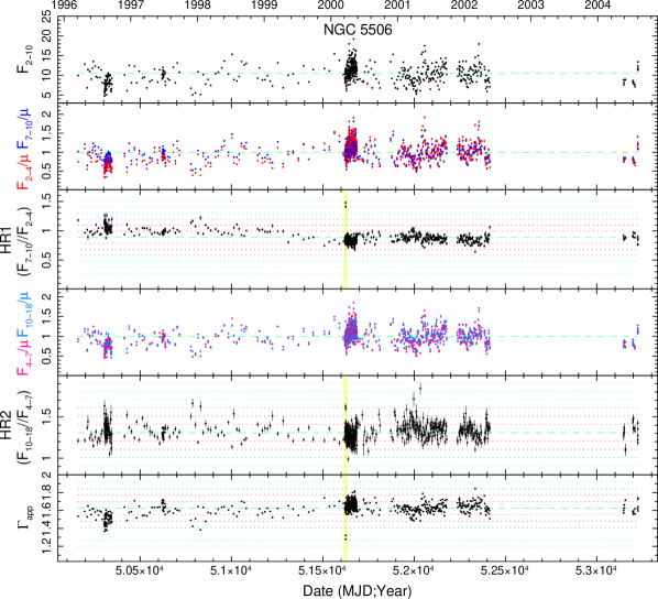
Figure A.18: Same as Fig. A.1, but for the Sy 1.9 NGC 5506. The yellow shaded area indicates a candidate eclipse event in 2000; see Fig. A.19 for a zoom-in on that period.

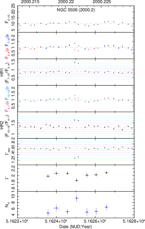
Figure A.19: Same as Fig. A.18, but a zoom-in on the eclipse event in 2000. The bottom two panels show $\Gamma$ and $N_{\rm H}$ in units of $10^{22}$ cm^-2.

A.8 Mkn 348 (Sy 2)

$\bullet$ 1996–1997 (“Secure A”): The long-term light curves are plotted in Fig. A.20. RXTE observed this source 25 times over a 16 d period in 1996 May–June, followed by sporadic observations from 1996 December through 1997 July. The source was monitored regularly once every two days during 2011 January – November followed by four times daily monitoring for 30 d in 2011 November–December. Our $HR1$ light curve shows a decrease from 5–8 in 1996 ($\sim$2–3$\sigma$) to 3 by 1997, with values $\sim$1.5–3 in 2011.

Smith et al. (2001) and Akylas et al. (2002), fitting spectra from the 1996–1997 campaigns, reported a steady decrease in $N_{\rm H}$ from $\sim$27 to 12 $\times 10^{22}$ cm^-2; they assumed $\Gamma$ frozen at 1.85 and angr abundances. We divide data from the 1996–1997 campaign into six coarse time slices, to confirm the decrease in $N_{\rm H}$, albeit with a larger time resolution. We assume a simple full-covering neutral absorber and used the best-fitting model from Rivers et al. (2013); we keep $R$ frozen at 0.3, and $I_{\rm Fe}$ frozen at $3\times 10^{-5}$ ph cm^-2 s^-1 (when we allow $I_{\rm Fe}$ to vary, values are almost always consistent with this value at the 90 per cent level). Assuming angr abundances, we obtain best-fitting values of $N_{\rm H}$($t$) consistent with Akylas et al. (2002; their fig. 2). Assuming wilm abundances instead, we obtain values of $N_{\rm H}$ an average of 1.42 higher. That is, we measure a decrease from $\sim 32$ to $\sim 20$ $\times 10^{22}$ cm^-2, as listed in Table 13.

We also perform spectral fits to the 2011 data, dividing them into three coarse time slices (MJD 55562–55647, 55684–55888, and 55890–55921), with the divisions corresponding to a sun-angle gap and the start of the intensive monitoring. We apply the same model as above, and we obtain best-fitting values of $N_{\rm H}$ of $\sim 15-17\times 10^{22}$ cm^-2 (using wilm abundances), with corresponding values of $\Gamma$ listed in Table 13.

As shown in Table 13, if we assume that the value of $N_{\rm H}$ throughout 1996–1997 was $16.6\times 10^{22}$ cm^-2 (the average of the three values obtained for 2011), we obtain fits for spectra # 1–5 with significantly worse values of $\chi^{2}_{\rm red}$, strong curvature in the data/model residuals, and values of $\Gamma$ as low as 1.2.

Spectral fits to an XMM-Newton EPIC observation in 2002 July performed by Brightman & Nandra (2011) yield $N_{\rm H}=13.1^{+0.7}_{-1.3}\times 10^{22}$ cm^-2 (with $\Gamma=1.68^{+0.07}_{-0.10}$, angr abundances, thus $\sim 18\times 10^{22}$ cm^-2 with wilm abundances), consistent with the idea that $N_{\rm H}$ has varied only weakly since 1997 July. Assuming the “baseline” $N_{\rm H}$ level is $\sim 15-18\times 10^{22}$ cm^-2 (wilm abundances), the XMM-Newton and 2011 RXTE data thus support the suggestion by Akylas et al. (2002) that RXTE just caught the tail end of the eclipse in 1997 July.

We assign a minimum duration of 399 d (from the start of the RXTE monitoring at MJD 50227 until the point when RXTE measured a value of $N_{\rm H}$ consistent with the “baseline” level, after MJD 50626. Using the peak value of $N_{\rm H}$ from spectrum #3 and a baseline level of $16.6\times 10^{22}$ cm^-2, we adopt $\Delta$$N_{\rm H}=18\pm 3\times 10^{22}$ cm^-2.

The Tartarus database of AGN X-ray spectra observed with ASCA indicates absorption by a column $\sim 10\times 10^{22}$ cm^-2 for an observation on 1995 August 4 (MJD 49933), suggesting an upper limit to the duration of 693 d. If the event happened to start immediately after the ASCA observation, and if it had an $N_{\rm H}$($t$) profile that was symmetric in time, then the event peak would likely have occurred in 1996 July, just after the 1996 RXTE observations started. If this is the case then RXTE was lucky enough to observe the approximate peak $N_{\rm H}$ value. We cannot rule out, however, that peak $N_{\rm H}$ occurred before the RXTE observations started and thus might be higher than that observed by RXTE.

Table 13: Results of time-resolved spectral fits to Mkn 348

Start–stop	Expo	$N_{\rm H}$, $\Gamma$ free					$N_{\rm H}$ frozen at $11.5\times 10^{23}$ cm-2
(MJD)	(ks)	$\chi^{2}_{\rm red}/dof$	$N_{\rm H}$	$\Gamma$	$A_{1}$	$F_{2-10}$	$\chi^{2}_{\rm red}/dof$	$\Gamma$
50227.05–50231.99 (#1)	28.8	1.48/46	$32.4^{+2.6}_{-2.5}$	$1.55\pm 0.06$	$5.5^{+0.9}_{-0.7}$	1.27	4.25/47	$1.20\pm 0.03$
50233.16–50237.03 (#2)	79.0	2.62/46	$34.7^{+2.6}_{-2.3}$	$1.59^{+0.06}_{-0.05}$	$4.1^{+0.6}_{-0.5}$	0.85	6.96/47	$1.19\pm 0.02$
50238.44–50243.35 (#3)	65.8	2.36/46	$35.1^{+2.7}_{-2.5}$	$1.55\pm 0.06$	$3.9\pm 0.4$	0.87	6.17/47	$1.15\pm 0.02$
50446.44–50528.99 (#4)	18.2	0.50/46	$34.4^{+6.5}_{-5.5}$	$1.59^{+0.15}_{-0.13}$	$3.6^{+1.5}_{-1.0}$	0.74	1.05/47	$1.19\pm 0.06$
50576.94–50598.06 (#5)	7.5	0.50/46	$27.1^{+4.0}_{-3.6}$	$1.66^{+0.11}_{-0.10}$	$7.1^{+2.1}_{-1.6}$	1.46	0.98/47	$1.40\pm 0.05$
50626.91–50641.07 (#6)	27.8	1.02/46	$19.5^{+1.0}_{-0.9}$	$1.71\pm 0.03$	$12.2\pm 1.0$	2.67	1.51/47	$1.63\pm 0.02$
55562.45–55646.78 (#7)	38.4	1.31/44	$14.8^{+2.3}_{-2.2}$	$1.69\pm 0.08$	$6.5^{+0.8}_{-0.7}$	1.64	1.32/45	$1.74\pm 0.04$
55685.99–55888.42 (#8)	75.2	0.72/44	$17.7^{+1.6}_{-1.5}$	$1.68\pm 0.05$	$7.1\pm 0.9$	1.71	0.73/45	$1.65\pm 0.03$
55890.93–55920.54 (#9)	124.0	1.16/44	$17.2^{+1.1}_{-1.0}$	$1.71\pm 0.04$	$8.7^{+0.8}_{-0.7}$	2.01	1.15/45	$1.69\pm 0.02$

Results of time-resolved spectroscopy for Mkn 348; see also Akylas et al. (2002) for spectral fits to the 1996–1997 data. Column densities, which are in units of $10^{22}$ cm^-2, refer to total observed columns, i.e., baseline level plus eclipsing cloud. $A_{1}$ is the 1 keV normalization of the power law in units of $10^{-3}$ ph cm^-2 s^-1 keV^-1. $F_{2-10}$ is the observed/absorbed model flux in units of $10^{-11}$ erg cm^-2 s^-1. $I_{\rm Fe}$ is frozen at $3\times 10^{-5}$ ph cm^-2 s^-1. Each spectral fit is performed using the 3–23 keV bandpass.

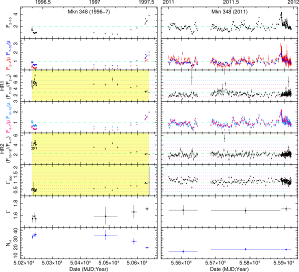
Figure A.20: Same as Fig. A.1, but for the Sy 2 Mkn 348. The yellow shaded area covers the 1996–1997 campaign and time-resolved spectroscopy indicating variations in $N_{\rm H}$ which have been published by Akylas et al. (2002). The bottom two panels indicate $\Gamma$ and $N_{\rm H}$ in units of $10^{22}$ cm^-2 from our time-resolved spectroscopic analysis, from fits where both parameters are free.

A.9 Additional objects with “candidate” events:

Fairall 9 (Sy 1), 2001.3 (“candidate”): The long-term light curve is plotted in Fig. A.21.

There is a small spike in $HR1$ over two consecutive points, at MJD 52029 and 52033 ($HR1_{\rm peak}\sim 1.3$ ; $>3\sigma$), plotted in Fig. A.22. However, the uncertainties are very high in each case ($\sim$0.3-0.5). $\Gamma_{\rm app}$ is roughly $1.2-1.4$ with uncertainties 0.06–0.08. We sum the two spectra together for spectral fitting, but the derived constraints are very poor: adopting the parameter values from the time-averaged fit from Rivers et al.  (2013), adding an extra column for neutral absorption using zphabs, and freezing $\Gamma$ to 2.0 yields $N_{\rm H}<2.1\times 10^{23}$ cm^-2. The event satisfies criteria 1–3, but with only an upper limit to $N_{\rm H}$ and with all continuum flux levels rather low, we classify this as a “candidate” event with a duration in the range 4–12 d .

$\bullet$ There are also two single point anomalously high values of $HR1$ at MJD 51257 and 51274 with values of $HR1$ and $\Gamma_{\rm app}$ similar to the above “candidate” event, but they fail criterion 2. Furthermore, spectral fitting to each spectrum yields $N_{\rm H}<4\times 10^{23}$ cm^-2, and so these events are rejected and not discussed further.

Lohfink et al. (2012) note the trio of low-flux “dips” in the 2–10 and 10–20 keV continuum light curves of Fairall 9 in mid- to late-2000 (MJD $\sim$ 51780, 51830, and 51860). They explore if these sudden decreases in the X-ray continuum flux could be associated with structural changes in the inner accretion disk or with absorption by Compton-thick clouds transiting the line of sight. However, our $HR1$ and $HR2$ light curves do not reveal anything obvious during mid- to late-2000: values are usually consistent with $\langle HR1\rangle$ or $\langle HR2\rangle$ and/or have large error bars and large point-to-point scatter.

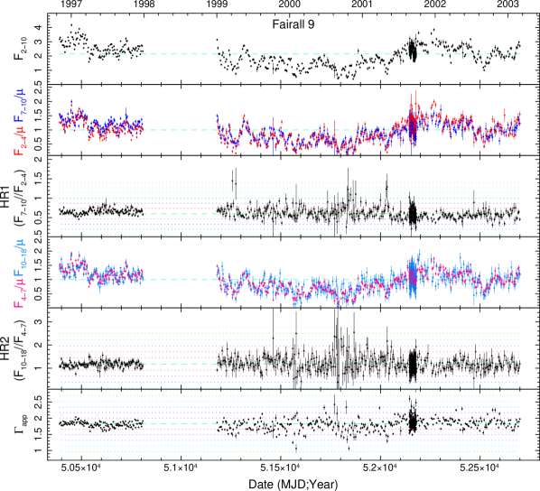
Figure A.21: Same as Fig. A.1, but for the Sy 1 Fairall 9.

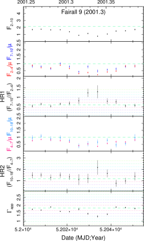
Figure A.22: Same as Fig. A.21, but a zoom-in on the ”candidate” event in 2001.

NGC 3516 (Sy 1.5), 2011.7, “candidate” event: This source’s $HR1$ light curve (Fig. A.23) shows systematic trends that are visually not obviously correlated with 2–10 or 10–18 keV continuum flux. Of peculiar interest is a ”spike” in $HR$ to $\sim$ 2.4 ($\sim 4\sigma$) during Fall 2011. $\Gamma_{\rm app}$ is usually 1.49$\pm$0.19 for NGC 3516 but reaches values as low as 0.8–0.9 in Fall 2011.

The X-ray spectrum of this object is commonly characterized by complex absorption, which can be variable on timescales of years, as documented by Turner et al. (2008). For example, Markowitz et al. (2008) found the source to be in a Compton-thin absorbed state in 2005. Turner et al. (2008), fitting Chandra HETGS and XMM-Newton EPIC and RGS spectra, list four ”zones” of absorption in addition to $N_{\rm H,Gal}$. Zone 3 (using their notation) is expected to impact modeling of PCA spectra of NGC 3516. This absorber is a partial-covering, moderately-ionized (log$\xi$ = 2.19) absorber; Turner et al. (2008) argue that variations in the covering fraction $CF$ on timescales of $\sim$ half a day can explain observed spectral variability. Rivers et al. (2011a), fitting the time-averaged PCA + HEXTE spectrum, modeled Zone 3 with log($\xi$) frozen at 2.19 and column density $N_{\rm H,WA}$ frozen at $2\times 10^{23}$ cm^-2, the best-fitting parameters from Turner et al. (2008), but leave the covering fraction $CF$ free, obtaining a best-fitting value of $CF=0.55\pm 0.10$.

For time-resolved spectroscopy, we sum the spectra from 2011 into five bins spanning approximately 80 d each; these spectra typically have exposure times of 11–22 ks and 25–50 $\times 10^{3}$ counts in the 3–23 keV band. We fit 3–23 keV spectra using the best-fitting model parameters from Rivers et al. (2011a), keeping log ($\xi$) and $N_{\rm H,WA}$ frozen at 2.19 for simplicity.

We test three simple models for the spectral variability: a model with $CF$ free, $\Gamma$ frozen at 1.85 (from Rivers et al. 2011a), and $N_{\rm H,WA}$ frozen at $2\times 10^{23}$ cm^-2 (which we call Model PC1); $\Gamma$ frozen at 1.85, $CF$ frozen at 0.75, and $N_{\rm H,WA}$ free (Model PC2); and $\Gamma$ free, $CF$ frozen at the arbitrary value of 0.75, and $N_{\rm H,WA}$ frozen at $2\times 10^{23}$ cm^-2 (Model PC3). $A_{1}$ and $I_{\rm Fe}$ are free parameters in all fits. The results are summarized in Table A8.

For Model PC1, best-fitting values of $CF$ span $0.34$ to $1.00$, with the highest value occurring for the Fall 2011 spectrum ($\#4$). However, uncertainties on $CF$ are extremely large; we also cannot rule out full-covering for spectrum $\#2$. Values of $\chi^{2}_{\rm red}$ between each of the three models were very similar and usually $\la$1. For model PC2, spectrum $\#4$ yields a value of $N_{\rm H,WA}$ about twice that for spectra $\#2$, 3 and 5, but $\chi^{2}_{\rm red}$ was 1.57, with strong data/model residuals (at the $\sim 10-20$ per cent level) below 4–5 keV.

For Model PC3, best-fitting values of $\Gamma$ are usually 1.7 and greater, with $\Gamma=1.55\pm 0.04$ for the Fall 2011 spectrum; such values are not implausible based on empirical grounds. Since we cannot rule out flattening of the primary power law as the driver behind the observed variations in $HR1$, we cannot confirm that variations in properties of the ionized absorber occurred. More definitive results can be obtained if this source is subjected to future long-term X-ray spectral monitoring using higher energy resolution and a wider bandpass than the PCA, such as eROSITA or the proposed Large Observatory For X-ray Timing.

We thus classify the Fall 2011 event as a “candidate” full-covering event, with a duration of $\sim 57$ d based on the points in the $HR1$ light curve above $1\sigma$ deviation. With best-fitting covering fractions of 74, 100, and 79 per cent before, during, and after the event, respectively, in Model PC1, we use a covering fraction of 23.5 per cent and assign $\Delta$$N_{\rm H}$ =(0.235 $\times$ $2\times 10^{23}$ cm^-2) = $4.7\times 10^{22}$ cm^-2.

Table 14: Results of time-resolved spectral fits to NGC 3516, 2011.7

Start–stop	Expo	Model PC1				Model PC2
(MJD)	(ks)	$\chi^{2}_{\rm red}$	$CF$	$A_{1}$	$F_{2-10}$	$\chi^{2}_{\rm red}$	$N_{\rm H,WA}$	$A_{1}$
		(44 $dof$)				(45 $dof$)
55561.55–55637.70 ($\#1$)	17.4	0.67	$0.34^{+0.10}_{-0.09}$	$6.3\pm 1.1$	4.60	0.76	$8.7^{+1.3}_{-2.0}$	$13.5\pm 0.4$
55641.58–55721.90 ($\#2$)	17.7	0.84	$0.84^{+0.16}_{-0.14}$	$12.8\pm 1.0$	2.55	1.02	$35\pm 5$	$11.4\pm 0.7$
55725.88–55769.57 ($\#3$)	10.8	0.50	$0.74^{+0.24}_{-0.18}$	$10.1\pm 1.3$	2.44	0.49	$28^{+7}_{-5}$	$10.0\pm 0.8$
55773.55–55873.27 ($\#4$)	22.2	0.98	$1.00^{+0.00}_{-0.08}$	$14.5^{+0.3}_{-0.4}$	2.01	1.57	$65^{+2}_{-4}$	$12.3\pm 0.3$
55877.52–55925.39 ($\#5$)	11.4	1.08	$0.79^{+0.19}_{-0.15}$	$13.4^{+1.2}_{-1.3}$	2.92	1.13	$30\pm 5$	$12.3\pm 0.9$

Start–stop	Model PC3
(MJD)	$\chi^{2}_{\rm red}$	$\Gamma$	$A_{1}$
	(45 $dof$)
55561.55–55637.70 ($\#1$)	1.53	$2.12\pm 0.03$	$30.3^{+0.9}_{-1.2}$
55641.58–55721.90 ($\#2$)	0.90	$1.78\pm 0.04$	$9.5\pm 0.7$
55725.88–55769.57 ($\#3$)	0.49	$1.86\pm 0.05$	$10.4^{+1.1}_{-1.0}$
55773.55–55873.27 ($\#4$)	1.03	$1.55\pm 0.04$	$5.0\pm 0.4$
55877.52–55925.39 ($\#5$)	1.11	$1.83\pm 0.04$	$11.8\pm 1.0$

Results of time-resolved spectroscopy for the 2011 campaign of NGC 3516. Each model incorporates a partial-covering absorber with log($\xi$)=2.19. Covering fraction $CF$ is free in Model PC1, and frozen at 0.75 in Models PC2 and PC3. $N_{\rm H,WA}$ is free in Model PC2 and frozen at $20\times 10^{22}$ cm^-2 in Models PC1 and PC3. $\Gamma$ is free in Model PC3, and frozen at 1.85 in Models PC1 and PC2. $N_{\rm H}$ is listed in units of $10^{22}$ cm^-2. $A_{1}$ is the 1 keV normalization of the covered power law only in units of $10^{-3}$ ph cm^-2 s^-1 keV^-1. $F_{2-10}$ is the observed/absorbed model flux in units of $10^{-11}$ erg cm^-2 s^-1; values for Models PC2 and PC3 were virtually identical to those for model PC1. $I_{\rm Fe}$ is left free, with best-fitting values and uncertainties typically $\sim 6\pm 3\times 10^{-5}$ ph cm^-2 s^-1 for Models PC1 and PC2 and typically $\sim 8\pm 4\times 10^{-5}$ ph cm^-2 s^-1 for Model PC3.

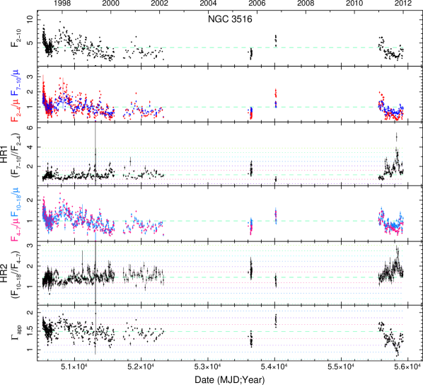
Figure A.23: Same as Fig. A.1, but for the Sy 1.5 NGC 3516.

A.10 Summary of eclipse events manifested via flux-flux plots

If there is an eclipse by a discrete cloud with $N_{\rm H}\sim 10^{22-23}$ cm^-2, as implied by the above spectral fits, then the 2–4 keV band should be impacted much more strongly than the 10–18 keV band. The 10–18 keV band probes the uneclipsed portion of the continuum power-law component in this case. In Figure A.24, we plot 2–4 keV flux as a function of 10–18 keV flux for each observation during each eclipse event, along with flux points representing non-eclipsed periods (the gray points). We use only the 75 data points before and after the putative eclipse (excluding other putative eclipse events) for clarity, to avoid overcrowding the figure. The green dashed line is a best fit to the gray points, using a linear regression algorithm that accounts for uncertainties in both quantities (Fasano & Vio 1988). The green dot-dashed lines indicate the $\pm 1\sigma$ distribution of the gray points. When there is no eclipse, the 2–4 and 10–18 keV bands are both probing the continuum and track variations in the power-law continuum. During each of the secure events, the flux-flux points track the spectral variability away from the main distribution, especially near the peak of each event. These plots do not directly yield quantitative information about $N_{\rm H}$ or $\Gamma$; those quantities are best obtained via time-resolved spectroscopy. However, these plots confirm that the 2–4 keV band is impacted independently of the behavior of the primary power law. For each of the candidate events, however, the low levels of 10–18 kev continuum flux (as indicated in bottom row of panels) introduce ambiguity in terms of our ability to use time-resolved spectroscopy to rule out flattening of the primary power law as the cause of observed spectral flattening.

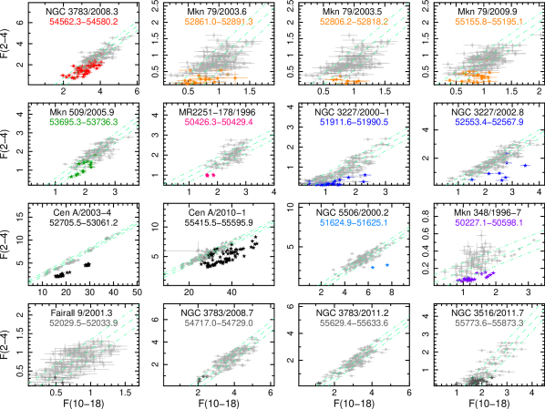
Figure A.24: 2–4 keV flux plotted against 10–18 keV flux for each observation during the secure/candidate eclipse events (colored stars) and for the 75 observations before and after each putative eclipse event (excluding other candidate/secure events; gray open circles). The 12 secure events are in the top three rows; the candidate events are in the bottom row. The green dashed line is a best fit to the non-eclipsed points, with the green dot-dashed lines indicating their $\pm 1\sigma$ distribution. For each of the secure events, the 2–4 keV band is affected independently of the 10–18 keV flux, indicating an eclipse by material with $N_{\rm H}\sim 10^{22-23}$ cm^-2. However, for each candidate event, there exists some ambiguity in modeling the spectral behavior, usually due to low flux in the power-law component (as probed by the 10–18 keV flux).

A.11 Type IIs with $\geq$0.6 years of monitoring

In Figs. A.25–A.30 we plot the long-term continuum and $HR1$ light curves for six type II objects with at least 0.6 years of sustained monitoring. X-ray spectral observations typically confirm the presence of an X-ray column $\ga 10^{22}$ cm^-2 in each of these objects (e.g., REN02). As hardness ratios are sensitive to changes in either $\Gamma$ or $N_{\rm H}$, the lack of any obvious systematic trends (above 2.0$\sigma$ from $\langle HR1\rangle$, and/or trends $\sim 50$ per cent greater than $\langle HR1\rangle$) suggests the lack of strong variations in either of these parameters. If we assume that $\Gamma$ is intrinsically constant, then we can use the average and 1$\sigma$ standard deviation of $HR1$ and the best-fitting time-averaged parameters from Rivers et al. (2013) to estimate the corresponding maximum change in $N_{\rm H}$; these estimates of $\Delta$$N_{\rm H}$ are listed in Table 15.

Table 15: Estimated sensitivity to $\Delta$$N_{\rm H}$ for type IIs based on $HR1$ light curves

			Typical	Typical	$\Delta$$N_{\rm H}$
Source	$\langle HR1\rangle$	$\sigma$	$N_{\rm H}$ ($10^{22}$ cm-2)	$\Gamma$	($10^{22}$ cm-2)
IRAS 04575–7537	0.56	0.06	$3.6\pm 2.6$ (R13)	$2.48\pm 0.22$ (R13)	$\sim 0.6$
Mkn 348 (2011 only)	2.35	0.84	$16.6\pm 1.6$ (TW); $\sim 11-16$ (R02)	$1.69\pm 0.06$ (TW)	$\sim 5$
NGC 1052	1.93	0.87	$13.6\pm 5.2$ (R13); $31^{+11}_{-26}$ (B11)	$1.71\pm 0.29$ (R13); $1.7^{+0.1}_{-0.2}$ (B11)	$\sim 6$
NGC 2992	0.84	0.17	0.4–1.6 (R02); $0.41\pm 0.17$ (B11)	$1.78\pm 0.18$ (R13); $1.59\pm 0.03$ (B11)	$\la 4$
NGC 4258	1.21	0.61	$8.4\pm 3.9$ (R13); $\sim 9-14$ (R02)	$1.80\pm 0.17$ (R13)	$\sim 5$
NGC 5506†	0.89	0.10	$1.9\pm 0.5$ (R11); $\sim 2-4$ (R02)	$1.93\pm 0.03$ (R11); $1.82^{+0.05}_{-0.04}$ (B11)	$\sim 1$
NGC 6251	0.36	0.49	$\la 0.4$ (G09)	$2.38\pm 0.23$ (R13); $1.67\pm 0.06$ (E06)	$\la 9$
NGC 7314	0.68	0.09	$\sim 0.8-1.3$ (R02); $0.60^{+0.01}_{-0.03}$ (B11)	$1.99\pm 0.10$ (R13); $1.95^{+0.02}_{-0.01}$ (B11)	$\sim 2$

Estimates of $\Delta$$N_{\rm H}$ corresponding to the standard deviations $\sigma$ of $HR1$. ^†For NGC 5506, the two observations at MJD 51624.94 and 51625.14 during an eclipse event are excluded. References for typical values of $\Gamma$ and $N_{\rm H}$ are: B11 = Brightman & Nandra (2011); E06 = Evans et al. (2006); G09 = González-Martín et al. (2009); R11 = Rivers et al. (2011a); R13 = Rivers et al. (2013); R02 = Risaliti, Elvis & Nicastro (2002) and references therein; TW = this work (Mkn 348: average of the three values derived from time-resolved fitting).

For NGC 4258, the average value of $HR1$ drops from 1.46 (stand. dev. 0.35) for the 1997–2000 data to 1.07 (stand. dev. 0.68) for the 2005–2011 data. While such a drop is consistent with the average values of $\Gamma$ or $N_{\rm H}$ systematically varying, spectral fitting on data summed over 1997–2000 and over 2005–2011 failed to provide evidence for changes in $\Gamma$ or $N_{\rm H}$, as uncertainties on these parameters were extremely large. Similarly, the average value of $HR1$ for NGC 5506 (Fig. A.18) also seems to fall very slightly towards the end of 1999: $\langle HR1\rangle$ = 1.03 (stand. dev. 0.08) for data before MJD 51300, and 0.85 (stand. dev. 0.06) for data after MJD 51500 (excluding the eclipse event covering the two observations at MJD 51624.94 and 51625.14). Spectral fitting on these two data sets, however, yields values of $N_{\rm H}$ consistent with the average at 90 per cent confidence.

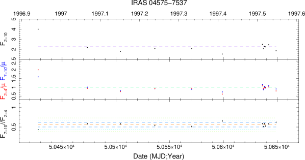
Figure A.25: Long-term continuum flux [$F_{\rm 2-10}$, top panel; $F_{\rm 2-4}$ (red) and $F_{\rm 7-10}$ (blue), middle panel] and $HR1$ light curves (bottom panel) for the Sy 2 IRAS 04575–7537.

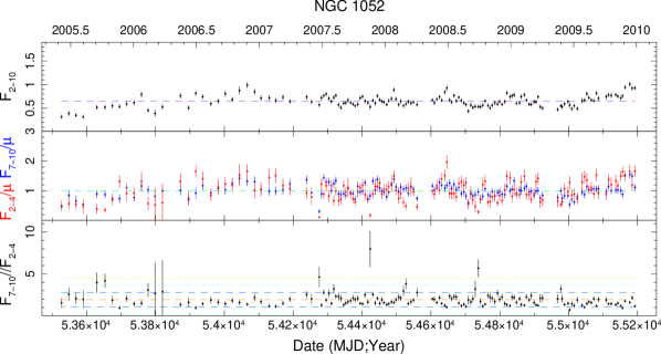
Figure A.26: Same as Fig. A.25, but for the radio-loud Sy 2 NGC 1052.

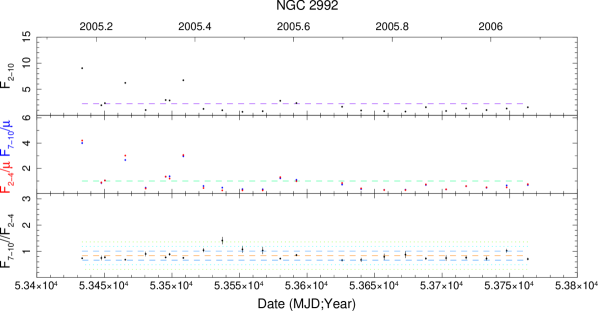
Figure A.27: Same as Fig. A.25, but for the Sy 2 NGC 2992.

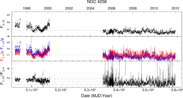
Figure A.28: Same as Fig. A.25, but for the Sy 2/LLAGN NGC 4258.

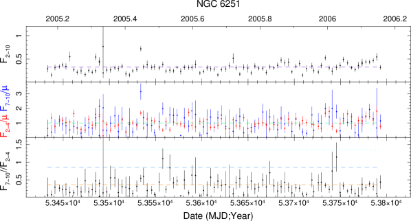
Figure A.29: Same as Fig. A.25, but for the Sy 2/LERG NGC 6251.

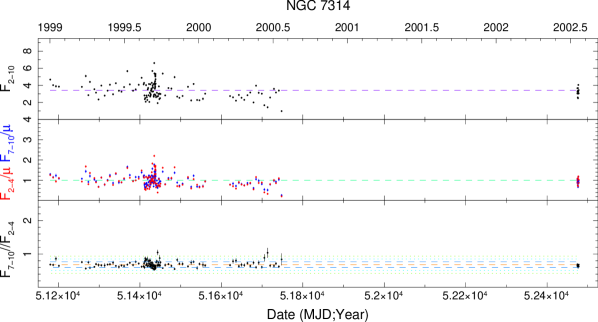
Figure A.30: Same as Fig. A.25, but for the Sy 1.9 NGC 7314.

Appendix B Inferred radial distances of various emission/absorption components in our eight primary sources

In this appendix, we provide the inferred distances from the central black hole of various emission/absorption components in our eight sources with “secure” eclipse events; Fig. 8 is based on these values. In Table B1, we list the X-ray clumps’ minimum and maximum distances as calculated in $\S$5.2: assuming a range of log($\xi$) from –1 to +1 for all events except for the two events in Cen A (log($\xi$) = –1 to 0) and NGC 3227/2000–1 (–0.3 to 0). We also list inferred locations of IR-emitting tori from either interferometry or reverberation mapping, BLR emission lines, and Fe K$\alpha$ line-emitting gas. The reader is reminded that even if distances from the black hole are commensurate, structures may not physically overlap (e.g., emission originating from out of the line of sight versus X-ray absorption along the line of sight).

Table 16: Inferred radial distances of various structures in objects with “secure” eclipses

Source	Component	Radius (light-days)	Radius ($R_{\rm g}$)	Ref.
NGC 3783	He ii	$1.4^{+0.8}_{-0.5}$	$850^{+480}_{-300}$	P04
	Si iv	$2.0^{+0.9}_{-1.1}$	$1210^{+550}_{-670}$	P04
	C iv	$3.8^{+1.0}_{-0.9}$	$2300^{+610}_{-550}$	P04
	H$\beta$	$10.2^{+3.3}_{-2.3}$	$6180^{+2000}_{-1390}$	P04
	He i$\lambda$2.058$\mu$	$14.7^{+4.7}_{-3.2}$	$8570^{+2740}_{-1870}$	R02
	Br$\gamma$ (broad)	$21.4^{+1.5}_{-1.3}$	$1.253^{+0.083}_{-0.075}\times 10^{4}$	R02
	Fe K$\alpha$ width, HETGS	$66^{+39}_{-20}$	$3.9^{+2.2}_{-1.2}\times 10^{4}$	S10
	IR torus (B08, Model A)	48–76	$2.8-4.4\times 10^{4}$	B08
	$H$-band-emitting dust	$66^{+6}_{-7}$	$3.9\pm 0.4\times 10^{4}$	L11
	$K$-band-emitting dust	$76^{+11}_{-17}$	$4.4^{+0.6}_{-1.0}\times 10^{4}$	L11
	X-ray clump	55–400	3.2–23 $\times 10^{4}$	This work
	$R_{\rm d}$	240	$13.9\times 10^{4}$	This work
	IR torus (B08, Model B)	250–357	$14.6-20.9\times 10^{4}$	B08
Mkn 79	Fe K$\alpha$ width, EPIC	$3.0^{+0.7}_{-0.8}$	$990^{+210}_{-240}$	Ga11
	H$\beta$	$9.0^{+8.3}_{-7.8}$	$3100^{+2800}_{-2600}$	P04
	H$\beta$	$16.0^{+6.4}_{-5.8}$	$5400^{+2200}_{-2000}$	P04
	H$\beta$	$16.1\pm 6.6$	$5500\pm 2200$	P04
	C iv	16.9	5590	K07
	Br$\gamma$	20.5	6750	L08
	H$\alpha$	23.3	7660	L08
	H$\beta$	26.4	8690	L08
	He i$\lambda$5876	27.9	9170	L08
	O i$\lambda$1.1287$\mu$	30.7	10090	L08
	Pa$\alpha$, Pa$\beta$, Pa$\delta$, Pa$\epsilon$	29.0–31.5	9530– 10360	L08
	O i$\lambda$8446	32.6	10720	L08
	He i$\lambda$1.0830$\mu$	57.1	18800	L08
	$R_{\rm d}$	340	$11.1\times 10^{4}$	This work
	X-ray clump	60–1020	$2.0-34\times 10^{4}$	This work
Mkn 509	He ii	$33.5^{+8.2}_{-7.1}$	$3870^{+950}_{-820}$	P04
	He i$\lambda$5876	59	6550	L08
	H$\beta$	68	7570	L08
	H$\beta$	$79.6^{+6.1}_{-5.4}$	$9190^{+700}_{-620}$	P04
	Pa$\alpha$, Pa$\beta$, Pa$\gamma$, Pa$\delta$, Pa$\epsilon$	93–120	10330–13340	L08
	O i$\lambda$8446	99	11020	L08
	H$\alpha$	100	11180	L08
	H$\gamma$	103	11450	L08
	Br$\gamma$	111	12390	L08
	He i$\lambda$1.0830$\mu$	119	13320	L08
	Fe K$\alpha$ line width, HETGS	$123^{+254}_{-89}$	$1.4^{+2.8}_{-1.0}\times 10^{4}$	S10
	O i$\lambda$1.1287$\mu$	126	14010	L08
	$R_{\rm d}$	610	$6.7\times 10^{4}$	This work
	X-ray clump	230–2800	2.6–31 $\times 10^{4}$	This work
MR 2251–178	Fe K$\alpha$ width, Suzaku	$>$9	$>$750	Go11
	H$\beta$	27	2300	S07
	C iv	$85^{+15}_{-13}$	$7230^{+1310}_{-1040}$	S07
	$R_{\rm d}$	910	$8.1\times 10^{4}$	This work
	X-ray clump	200–2500	1.7–120 $\times 10^{4}$	This work

Table 1: Inferred radial distances of various structures in objects with “secure” eclipses, continued

Source	Component	Radius (light-days)	Radius ($R_{\rm g}$)	Ref.
NGC 3227	He i$\lambda$5876	2.0	4580	L08
	H$\beta$	3.4	7640	L08
	Pa$\epsilon$	3.4	7690	L08
	H$\gamma$	3.7	8330	L08
	O i$\lambda$8446	4.0	8980	L08
	H$\beta$	$3.8\pm 0.8$	$9000\pm 1890$	D10
	Br$\gamma$	4.0	9010	L08
	H$\alpha$	4.4	10010	L08
	O i$\lambda$1.1287$\mu$	4.9	11220	L08
	He i$\lambda$1.0830$\mu$	5.7	12860	L08
	Pa$\beta$, Pa$\delta$	6.0	13600	L08
	Fe K$\alpha$ width, EPIC	$7.2^{+12.7}_{-4.9}$	$1.7^{+3.0}_{-1.2}\times 10^{4}$	M09
	H$\alpha$	$18.9^{+8.7}_{-11.3}$	$4.48^{+2.06}_{-2.68}\times 10^{4}$	P04
	$K$-band-emitting dust	$\sim$20	$4.74\times 10^{4}$	S06
	X-ray clump	6.5–91	$1.5-21\times 10^{4}$	This work
	$R_{\rm d}$	85	$19.2\times 10^{4}$	This work
	Fe K$\alpha$ variability	$<$ 700	$<1.7\times 10^{6}$	M09
Cen A	$R_{\rm d}$	42	$1.22\times 10^{4}$	This work
	Fe K$\alpha$ width, Suzaku	$>$ 66	$>1.9\times 10^{4}$	Ma07
	IR Torus	120–360	3.5–11 $\times 10^{4}$	Me07
	X-ray clump	94–710	2.7–20 $\times 10^{4}$	This work
NGC 5506	X-ray clump	15–220	$0.3-4.4\times 10^{4}$	This work
	Pa$\beta$	$\sim$190	$3.7\times 10^{4}$	N02
	Fe K$\alpha$ width, HETGS	$220^{+764}_{-127}$	$4.4^{+15.2}_{-2.5}\times 10^{4}$	S10 (68$\%$ err.)
	$R_{\rm d}$	240	$4.8\times 10^{4}$	This work
	Br$\gamma$	$250^{+40}_{-30}$	$5.0^{+0.7}_{-0.6}\times 10^{4}$	N02
	Br$\alpha$	$420^{+70}_{-60}$	$8.3^{+1.6}_{-1.2}\times 10^{4}$	L02
Mkn 348	H$\beta$	$1.19\pm 0.03$	1340$\pm$30	T95
	H$\alpha$	$1.47^{+0.10}_{-0.11}$	$1650^{+130}_{-110}$	T95
	Br$\gamma$	$\sim$ 16.6	$1.87\times 10^{4}$	V97
	Pa$\beta$	$\sim$ 30.4	$3.42\times 10^{4}$	V97
	$R_{\rm d}$	235	$26.8\times 10^{4}$	This work
	X-ray Clump	140–1290	$16-150\times 10^{4}$	This work

For BLR line lags from reverberation mapping (P04, D10), $\tau_{\rm cent}$ is used if available. For Mkn 79, we use “unflagged” H$\beta$ values only. $R_{\rm d}$ denotes the approximate outer boundary of the DSZ, i.e., dust residing at distances greater than $R_{\rm d}$ likely does not sublimate, while distances smaller than $\sim\frac{1}{2}-\frac{1}{3}R_{\rm d}$ are likely to be dust-free. References for Column (5) are: B08 = Beckert et al. (2008), D10 = Denney et al. (2010), Ga11 = Gallo et al. (2011), Go11 = Gofford et al. (2011), K07 = Kelly & Bechtold (2007), L02 = Lutz et al. (2002), L08 = Landt et al. (2008), L11 = Lira et al. (2011), Ma07 = Markowitz et al.  (2007), M09 = Markowitz et al. (2009), Me07 = Meisenheimer et al.  (2007), N02 = Nagar et al. (2002), P04 = Peterson et al. (2004), R03 = Reunanen et al. (2003), S06 = Suganuma et al. (2006), S07 = Sulentic et al. (2007), S10 = Shu et al. (2010; 68 per cent uncertainties used), T95 = Tran (1995), V97 = Veilleux et al. (1997).

References

- (1) Abdo, A.A., et al. 2010, ApJ, 719, 1433
- (2) Akylas A., Georgantopoulos I., Griffiths R.G., Papadakis I.E., Mastichiadis A., Warwick R.S., Nandra K., Smith D.A., 2002, MNRAS, 332, L23
- (3) Alonso-Herrero A., et al. 2011, ApJ, 736, 82
- (4) Anders E., Grevesse N., 1989, Geochim. Cosmochim. Acta, 53, 197
- (5) Antonucci R.R.J., Miller J.S., 1985, ApJ, 297, 621
- (6) Arévalo P., Uttley P., Kaspi S., Breedt E., Lira P., McHardy I.M., 2008, MNRAS, 389, 1479
- (7) Aretxaga I., Joguet B., Kunth D., Melnick J., Terlevich R.J., 1999, ApJ, 519, L123
- (8) Asensio Ramos A., Ramos Almeida C., 2009, ApJ, 696, 2075
- (9) Awaki H. et al., 2008, PASJ, 60S, 293
- (10) Barr P., White N.E., Sanford P.W., Ives J.C., 1977, MNRAS, 181, 43P
- (11) Barth A., Filippenko A.V., Moran E.C., 1999, ApJ, 515, L61
- (12) Beckert T., Dribe T., Hönig S.F., Weigelt G., 2008, A&A, 486, L17
- (13) Bianchi S., Guainazzi M., 2007, in Antonelli, L.A., et al., eds, AIP Conf. Ser. Vol. 924, The Multicolored Landscape of Compact Objects and Their Explosive Origins, Am. Inst. Phys., New York, p. 822
- (14) Bianchi S., Piconcelli E., Chiaberge M., Bailón E.J., Matt G., Fiore F., 2009, ApJ, 695, 781
- (15) Breedt E. et al., 2009, MNRAS, 394, 427
- (16) Brightman M., Nandra K., 2011, MNRAS, 413, 1206
- (17) Burtscher L., Meisenheimer K., Jaffe W., Tristram K.R.W., Röttgering H.J.A., 2010, PASA, 27, 290
- (18) Chartas G., Kochanek C.S., Dai X., Moore D., Mosquera A.M., Blackburne J.A., 2012, ApJ, 757, 137
- (19) Chatterjee R. et al., 2011, ApJ, 734, 43
- (20) Chen B., Dai X., Kochanek C.S., Chartas G., Blackburne J.A., Morgan C.W., 2012, ApJ, 755, 24
- (21) Chiaberge M., Capetti A., Celotti A., 2001, MNRAS, 324, L33
- (22) Cohen R.D., Puetter R.C., Rudy R.J., Ake T.B., Foltz C.B., 1986, ApJ, 311, 135
- (23) Collmar W. et al., 2010, A&A, 522, A66
- (24) Czerny B., Hryniewicz K., 2011, A&A, 525, L8
- (25) Dadina M., 2007, A&A, 461, 1209
- (26) Dapp W.B., Basu S., 2009, MNRAS, 395, 1092
- (27) Denney K.D. et al., 2010, ApJ, 721, 715
- (28) de Rosa A., Piro L., Perola G.C., Capalbi M., Cappi M., Grandi P., Maraschi L., Petrucci P.O., 2007, A&A, 463, 903
- (29) Done C., Gierliński M., 2005, MNRAS, 364, 208
- (30) Dorodnitsyn A., Kallman T., 2012, ApJ, 761, 70
- (31) Dorodnitsyn A., Kallman T., Bisnovatyi-Kogan G.S., 2012, ApJ, 747, 8
- (32) Driver S.P., Popescu C.C., Tuffs R.J., Liske J., Graham A.W., Allen P.D., de Propris R., 2007, MNRAS, 379, 1022
- (33) Ebneter K., Balick B., 1983, PASP, 95, 675
- (34) Elitzur M., 2007, in Ho. L.C., Wang, J.-M., eds, ASP Conf. Ser. Vol. 373, The Central Engine of Active Galactic Nuclei, Astron. Soc. Pac., San Francisco, p. 415
- (35) Elitzur M., Ho L.C., 2009, ApJ, 701, L91
- (36) Elitzur M., Shlosman I., 2006, ApJ, 648, L101
- (37) Elvis M., 2012, J. Phys. Conf. Ser., 372, 012032
- (38) Evans D.A., Worrall D.M., Hardcastle M.J., Kraft R.P., Birkinshaw M., 2006, ApJ, 642, 96
- (39) Evans I.N., Ford H.C., Kriss G.A., Tsvetanov Z., 1994, in Bicknell G.V., Dopita, M.A., Quinn P.J., eds, ASP Conf. Ser. Vol. 54, The First Stromlo Symposium: The Physics of Active Galaxies, Astron. Soc. Pac., San Francisco, p. 3
- (40) Fasano G., Vio R., 1988, Bull. Inf. Cent. Données Stellaires, 35, 191
- (41) Fukumura K., Kazanas D., Contopoulos I., Behar E., 2010, ApJ, 715, 636
- (42) Gallo L.C., Miniutti G., Miller J.M., Brenneman L.W., Fabian A.C., Guainazzi M., Reynolds C.S., 2011, MNRAS, 411, 607
- (43) Garcet O. et al., 2007, A&A, 474, 473
- (44) Gaskell C.M., Goosmann R.W., Klimek E.S., 2008, Mem. Soc. Astron. Ital., 79, 1090
- (45) Gibson R.R., Marshall H.L., Canizares C.R., Lee J.C., 2005, ApJ, 627, 83
- (46) Gofford J. et al., 2011, MNRAS, 414, 3307
- (47) González-Martín O. et al., 2009, A&A, 506, 1107
- (48) Goodrich R.W., 1989, ApJ, 340, 190
- (49) Goodrich R.W., Veilleux S., Hill G.J., 1994, ApJ, 422, 521
- (50) Haardt F., Maraschi L., Ghisellini G., 1997, ApJ, 432, L95
- (51) Hao L., Weedman D.W., Spoon H.W.W., Marshall J.A., Levenson N.A., Elitzur M., Houck J.R., 2007, ApJ, 655, L77
- (52) Herrnstein J. et al., 1999, Nature, 400, 539
- (53) Holt S.S., Mushotzky R.F., Boldt E.A., Serlemitsos P.J., Becker R.H., Szymkowiak A.E., White N.E., 1980, ApJ, 241, L13
- (54) Hönig S.F., 2013, in Packham C., Mason R., Alonso-Herrero A., eds, Proc. of the Torus Workshop 2012, San Antonio, preprint (arXiv:1301.1349)
- (55) Horst H., Smette A., Gandhi P., Duschl W.J., 2006, A&A, 457, L17
- (56) Hunt L.K., Malkan M.A., Rush B., Bicay M.D., Nelson B.O., Stanga R.M., Webb, W., 1999, ApJS, 125, 349
- (57) Jaffe W. et al., 2004, Nature, 429, 47
- (58) Jahoda K., Markwardt C.B., Radeva Y., Rots A.H., Stark M.J., Swank J.H., Strohmayer T.E., Zhang W., 2006, ApJS, 163, 401
- (59) Jarrett T.H., Chester T., Cutri R., Schneider S.E., Huchra J.P., 2003, AJ, 125, 525
- (60) Kalberla P.M.W. et al., 2005, A&A, 440, 775
- (61) Kaspi S., Netzer H., Chelouche D., George I.M., Nandra K., Turner T.J., 2004, ApJ, 611, 68
- (62) Kelly B.C., Bechtold J., 2007, ApJS, 168, 1
- (63) Kishimoto M., Hönig S.F., Antonucci R., Barvainis R., Kotani T., Tristram K., Weigelt G., Levin K., 2011, A&A, 527, A121
- (64) Kishimoto M., Hönig S.F., Antonucci R., Kotani T., Barvainis R., Tristram K., Weigelt G., 2009, A&A, 507, L57
- (65) Konigl A., Kartje J.F., 1994, ApJ, 434, 446
- (66) Krawczynski H., Coppi P.S., Aharonian F., 2002, MNRAS, 336, 721
- (67) Krolik J., 2007, ApJ, 661, 52
- (68) Krolik J., Begelman M.C., 1986, ApJ, 308, L55
- (69) Krolik J., Begelman M.C., 1988, ApJ, 329, 702
- (70) Lamer G., Uttley P., McHardy I.M., 2003, MNRAS, 342, L41
- (71) Landt H., Bentz M.C., Ward M.J., Elvis M., Peterson B.M., Korista K.T., Karovska M., 2008, ApJS, 174, 282
- (72) Lasota J.-P., Abramowicz M.A., Chen X., Krolik J., Narayan R., Yi I., 1996, ApJ, 462, L142
- (73) Lira P., Ward M.J., Zezas A., Murray S.S., 2002, MNRAS, 333, 709
- (74) Lira P., Arévalo P., Uttley P., McHardy I., Breedt E., 2011, MNRAS, 415, 1290
- (75) Lohfink A., Reynolds C.S., Mushotzky R.F, Wilms J., 2012, ApJ, 749, L31
- (76) Lumsden S.L., Alexander D.M., Hough J.H., 2004, MNRAS, 348, 1451
- (77) Lutz D., Maiolino R., Moorwood A.F.M., Netzer H., Wagner S.J., Sturm E., Genzel R., 2002, A&A, 396, 439
- (78) Lutz D., Maiolino R., Spoon H.W.W., Moorwood A.F.M., 2004, A&A, 418, 465
- (79) Maiolino R., Marconi A., Salvati M., Risaliti G., Severgnini P., Oliva E., La Franca F., Vanzi, L., 2001, A&A, 365, 28
- (80) Maiolino R. et al., 2010, A&A, 517, A47
- (81) Malkan M.A., Gorjian V., Tam R., 1998, ApJS, 117, 25
- (82) Marconi A., Risaliti G., Gilli R., Hunt, L.K., Maiolino R., Salvati M., 2004, MNRAS, 351, 169
- (83) Markoff S., Nowak M.A., Wilms J., 2005, ApJ, 635, 1203
- (84) Markowitz A. et al., 2003, ApJ, 593, 96
- (85) Markowitz A. et al., 2007, ApJ, 665, 209
- (86) Markowitz A. et al., 2008, PASJ, 60, S277
- (87) Markowitz A., Reeves J.N., George I.M., Braito V., Smith R., Vaughan S., Arévalo P., Tombesi F., 2009, ApJ, 691, 922
- (88) Mateos S. et al., 2010, A&A, 510, A35
- (89) McClintock J.E., Remillard R.A., 2003, in ”Compact Stellar X-ray Sources,” eds. Lewin W.H.G., van der Klis M., Cambridge University Press (astro-ph/0306213)
- (90) McHardy I.M., Koerding E., Knigge C., Uttley P., Fender R.P. 2006, Nature, 444, 730
- (91) Meisenheimer K. et al., 2007, A&A, 471, 453
- (92) Miller J.S., Goodrich R.W., 1990, ApJ, 355, 456
- (93) Minezaki T., Yoshii Y., Kobayashi Y., Enya K., Suganuma M., Tomita H., Aoki T., Peterson B.A., 2004, ApJ, 600, L35
- (94) Miniutti G., et al., 2014, MNRAS, 437, 1776
- (95) Miyoshi M., Moran J., Herrnstein J., Greenhill L., Nakai N., Diamond P., Inoue M., 1995, Nature, 373, 127
- (96) Moran E.C., Barth A., Kay L.E., Filippenko A.V., 2000, ApJ, 540, L73
- (97) Nagar N.M., Oliva E., Marconi A., Maiolino R., 2002, A&A, 391, L21
- (98) Nandra K., Le T., George I.M., Edelson R.A., Mushotzky R.F., Peterson B.M., Turner T.J., 2000, ApJ, 544, 734
- (99) Nenkova M., Sirocky M., Ivezić Ž., Elitzur M., 2008a, ApJ, 685, 147
- (100) Nenkova M., Sirocky M., Nikutta R., Ivezić Ž., Elitzur M., 2008b, ApJ, 685, 160
- (101) Netzer H., Laor A., 1993, ApJ, 404, L51
- (102) Nikutta R., Elitzur M., Lacy M., 2009, ApJ, 707, 1550
- (103) Osterbrock D.E., 1981, ApJ, 249, 462
- (104) Papadakis I.E., 2004, MNRAS, 348, 207
- (105) Papadakis I.E., Petrucci P.O., Maraschi L., McHardy I.M., Uttley P., Haardt F., 2002, ApJ, 573, 92
- (106) Patrick A.R., Reeves J.N., Porquet D., Markowitz A., Braito V., Lobban A.P., 2012, MNRAS, 426, 2522
- (107) Perola G.C. et al., 2004, A&A, 421, 491
- (108) Peterson B.M. et al., 2004, ApJ, 613, 682
- (109) Poncelet A., Perrin G., Sol H., 2006, A&A, 450, 483
- (110) Pott J.-U., Malkan M.A., Elitzur M., Ghez A.M., Herbst T.M., Schödel R., Woillez, J., 2010, ApJ, 713, 736
- (111) Predehl P., Schmidt J., 1995, A&A, 293, 889
- (112) Predehl P. et al., 2011, Proc. SPIE, 8145, 247
- (113) Puccetti S., Fiore F., Risaliti G., Capalbi M., Elvis M., Nicastro F., 2007, MNRAS, 377, 607
- (114) Raban D., Jaffe W., Röttgering H., Meisenheimer K., Tristram K., 2009, MNRAS, 394, 1325
- (115) Ramos Almeida C. et al., 2009, ApJ, 702, 1127 (RA09)
- (116) Ramos Almeida C. et al., 2011, ApJ, 731, 92 (RA11)
- (117) Reeves J.N., Turner M., 2000, MNRAS, 316, 234
- (118) Reeves J.N., Nandra K., George I.M., Pounds K., Turner T.J., Yaqoob T., 2004, ApJ, 602, 648
- (119) Reis R.C., Miller, J.M., 2013, ApJ, 769, L7
- (120) Reunanen J., Kotilainen J.K., Prieto M.A., 2003, MNRAS, 343, 192
- (121) Risaliti G., Elvis M., Nicastro F., 2002, ApJ, 571, 234 (REN02)
- (122) Risaliti G., Elvis M., Fabbiano G., Baldi A., Zezas A., 2005, ApJ, 623, L93
- (123) Risaliti G., Elvis M., Fabbiano G., Baldi A., Zezas A., Salvati M., 2007, ApJ, 659, L111
- (124) Risaliti G. et al., 2009a, MNRAS, 393, L1
- (125) Risaliti G. et al., 2009b, ApJ, 696, 160
- (126) Risaliti G., Nardini E., Salvati M., Elvis E., Fabbiano G., Maiolino R., Pietrini P., Torricelli-Ciamponi G., 2011, MNRAS, 410, 1027
- (127) Rivers E.S., Markowitz A., Rothschild R.E., 2011a, ApJS, 193, 3
- (128) Rivers E.S., Markowitz A., Rothschild R.E., 2011b, ApJ, 742, L29
- (129) Rivers E.S., Markowitz A., Rothschild R.E., 2013, ApJ, 772, 114
- (130) Rothschild R.E., Markowitz A., Rivers E.S., Suchy S., Pottschmidt K., Kadler M., Müller C., Wilms J., 2011, ApJ, 733, 23
- (131) Roustazadeh P., Böttcher M., 2011, ApJ, 728, 134
- (132) Sanfrutos M., Miniutti G., Agís-González B., Fabian A.C., Miller J.M., Panessa F., Zoghbi A., 2013, MNRAS, 436, 1588
- (133) Schartmann M., Meisenheimer K., Camenzind M., Wolf S., Henning T., 2005, A&A, 437, 861
- (134) Schurch N., Warwick R.S., 2002, MNRAS, 334, 811
- (135) Shao Z., Xiao Q., Shen S., Mo H.J., Xia X., Deng Z., 2007, ApJ, 659, 1159
- (136) Shih D.C., Iwasawa K., Fabian A.C., 2002, MNRAS, 333, 687
- (137) Shu X.W., Yaqoob T., Wang J.X., 2010, ApJS, 187, 581
- (138) Smith D.A., Georgantopoulos I., Warwick R.S., 2001, ApJ, 550, 635
- (139) Sobolewska M.A., Papadakis I.E., 2009, MNRAS, 399, 1597
- (140) Soldi S. et al., 2008, A&A, 486, 411
- (141) Stalevski M., Fritz, J., Baes M., Nakos T., Popović L., 2012, MNRAS, 420, 2756
- (142) Steinle H., 2010, PASA, 27, 431
- (143) Sturm E. et al., 2005, ApJ, 629, L21
- (144) Suganuma M. et al., 2006, ApJ, 639, 46
- (145) Sulentic J.W., Bachev R., Marziani P., Negrete C.A., Dultzin D., 2007, ApJ, 666, 757
- (146) Taylor R.D., Uttley P., McHardy I.M., 2003, MNRAS, 342, L31
- (147) Tran H.D., 1995, ApJ, 440, 565
- (148) Tran H.D., Osterbrock D.E., Martel A., 1992, AJ, 104, 2072
- (149) Tristram K. et al., 2007, A&A, 474, 837
- (150) Tristram K. et al., 2009, A&A, 502, 67
- (151) Turner T.J., Reeves, J.N., Kraemer, S.B., Miller L., 2008, A&A, 483, 161
- (152) Urry C.M., Padovani P., 1995, PASP, 107, 803
- (153) Vasudevan R.V., Fabian A.C., 2009, MNRAS, 392, 1124
- (154) Vasudevan R.V., Fabian A.C., Gandhi P., Winter L.M., Mushotzky R.F., 2010, MNRAS, 402, 1081
- (155) Veilleux S., Goodrich R.W., Hill G.J., 1997, ApJ, 477, 631
- (156) Verner D.A., Ferland G.J., Korista K.T., Yakovlev D.G., 1996, ApJ, 465, 487
- (157) Vestergaard M., Peterson B.M., 2006, ApJ, 641, 689
- (158) Wang J., Mao Y.F., Wei J.Y., 2009, AJ, 137, 3388
- (159) Wang J.-M., Zhang E.-P., 2007, ApJ, 660, 1072
- (160) Wilms J., Allen A., McCray R., 2000, ApJ, 542, 914
- (161) Woo J.-H., Urry C.M., 2002, ApJ, 579, 530
- (162) Yang Y., Wilson A.S., Matt G., Terashima Y., Greenhill, L.J., 2009, ApJ, 691, 131