Self-energy correction to dynamic polaron response

Abstract

We present the first order self-energy correction to the linear response coefficients of polaronic systems within the truncated phase space approach developed by the present authors. Due to the system-bath coupling, the external pertubation induces a retarded internal field which dynamically screens the external force. Whereas the effect on the mobility is of second order, dynamical properties such as the effective mass and the optical absorption are modified in first order. The Fröhlich polaron is used to illustrate the results.

I Introduction

In a previous paper cit:SelsBrosensTruncate we presented an approximate, however systematically improvable, truncation method to derive the linear response coefficients from the quantum Liouville equation for the reduced Wigner function cit:SBreducedLiouville2013 of polaronic systems. The paper mainly addressed the discrepancy between the mobility of the Fröhlich polaron cit:Frohlich1937 ; cit:Frohlich1950 ; cit:Frohlich1954 proposed by Feynman et al. cit:FHIP1962   (hereafter referred to as FHIP) and Kadanoff cit:FHIP1962 . It was shown how a slight modification to each of the two methods, which accounts for their discrepancy and amends their problems, makes them compatible with the presented truncation method. Moreover, the new result turned out to be in agreement with a prediction made by Los’ cit:LOS .

In the present paper we concentrate on the dynamic response properties of the polaron system

$$H=\frac{\mathbf{p}^{2}}{2m}-e\mathbf{E(}t\mathbf{)}\cdot\mathbf{x}+\sum_{\mathbf{k}}\hbar\omega_{\mathbf{k}}\left(b_{\mathbf{k}}^{\dagger}b_{\mathbf{k}}+\frac{1}{2}\right)\\ +\sum_{\mathbf{k}}\left[\gamma(\mathbf{k})\exp\left(i\mathbf{k\cdot x}\right)b_{\mathbf{k}}^{\dagger}+\gamma^{\ast}(\mathbf{k})\exp\left(-i\mathbf{k\cdot x}\right)b_{\mathbf{k}}\right],$$ (I.1)

where $\left(\mathbf{x,p}\right)$ represents the particle which is coupled to some bosonic field $b_{\mathbf{k}}$ in a isotropic translational invariant way, i.e. $\gamma(\mathbf{k})=\gamma(\left|\mathbf{k}\right|)$ and $\omega_{\mathbf{k}}=\omega_{\left|\mathbf{k}\right|}$. The particle, which we consider to be charged, is subject to a small time dependent electric field $\mathbf{E(}t\mathbf{)}$ and we are concerned with finding the time dependent response of the system in the form of the conductivity

$$\mathbf{J}(t)=\int_{-\infty}^{t}\sigma(t-s)\mathbf{E(}s\mathbf{)}\mathrm{d}s=\frac{e}{m}\int\mathbf{p}f\left(\mathbf{p},t\right)\mathrm{d}\mathbf{p,}$$ (I.2)

where $f\left(\mathbf{p},t\right)$ is the reduced momentum distribution of the system.

II Self-energy correction and dynamical screening

Following Ref. cit:SelsBrosensTruncate we wish to derive an equation of motion for the current density under the assumption that the bosonic field $b_{\mathbf{k}}$ was initially in thermal equilibrium. It follows from definition (I.2) and from the relevant equations (2.5-2.7) of Ref. cit:SelsBrosensTruncate that the current density satisfies

$$\frac{d\mathbf{J}(t)}{dt}-\frac{e^{2}}{m}\mathbf{E(}t\mathbf{)}=-\sum_{k}\frac{2\left|\gamma(\mathbf{k})\right|^{2}}{\hbar}\mathbf{\mathbf{k}}\frac{e}{m}\int\mathrm{d}\mathbf{p}\int_{-\infty}^{t}dt^{\prime}\\ \times\left\{\begin{array}[c]{c}n_{B}(\omega_{k})\sin\left[\left(\frac{\mathbf{\hbar\mathbf{k}}^{2}}{2m}-\omega_{k}\right)(t-t^{\prime})\right]\\ +\left(n_{B}(\omega_{k})+1\right)\sin\left[\left(\frac{\mathbf{\hbar\mathbf{k}}^{2}}{2m}+\omega_{k}\right)(t-t^{\prime})\right]\end{array}\right\}\\ \times\sin\left(\mathbf{k\cdot}\left[\frac{\mathbf{p}}{m}(t-t^{\prime})+\int_{t^{\prime}}^{t}\int_{t^{\prime}}^{\tau}\frac{e\mathbf{E}(s)}{m}\mathrm{d}s\mathrm{d}\tau\right]\right)f\left(\mathbf{p},t^{\prime}\right).$$ (II.1)

At low temperature and for weak coupling, the momentum distribution function is assumed to be peaked around a small average value of $\mathbf{p}$, because the perturbation $\mathbf{E}$ is assumed to be weak. It thus seems reasonable to expand the sine function. Truncating the expansion up to first order results in

$$\frac{\partial}{\partial t}\mathbf{J}(t)+\int_{-\infty}^{t}\chi(t-s)\mathbf{J}(s)\mathrm{d}s=\frac{e^{2}}{m}\mathbf{E(}t\mathbf{)}\\ \mathbf{-}\frac{e^{2}}{m}\int_{-\infty}^{t}\kappa(t-s)\mathbf{E}(s)\mathrm{d}s,$$ (II.2)

where we have adopted the notation of cit:SelsBrosensTruncate , such that memory function $\chi$ of the system is given by

$$\chi(t)=t\sum_{k}\frac{2\left|\gamma(\mathbf{k})\right|^{2}}{3\hbar}\frac{\mathbf{\mathbf{k}}^{2}}{m}\\ \times\left\{\begin{array}[c]{c}n_{B}(\omega_{k})\sin\left(\left[\frac{\hbar\mathbf{k}^{2}}{2m}-\omega_{k}\right]t\right)\\ +\left(n_{B}(\omega_{k})+1\right)\sin\left(\left[\frac{\hbar\mathbf{k}^{2}}{2m}+\omega_{k}\right]t\right)\end{array}\right\},$$

and the polarizability $\kappa$ becomes

$$\kappa(t)=t\int_{t}^{\infty}\mathrm{d}\tau\frac{\chi(\tau)}{\tau}.$$ (II.3)

Consequently, according to Eq. (I.2), the Laplace transform $\mathcal{L}\left(\sigma,\Omega\right)$ of the conductivity satisfies

$$\mathcal{L}\left(\sigma,\Omega\right)=\frac{e^{2}}{m}\frac{1-\mathcal{L}\left(\kappa,\Omega\right)}{\Omega+\mathcal{L}\left(\chi,\Omega\right)}.$$ (II.4)

A more accurate conductivity can be found using a resummation argument similar to that in cit:SBreducedLiouville2013 , which yields

$$\mathcal{L}\left(\sigma,\Omega\right)\approx\frac{e^{2}}{m}\frac{1}{\Omega+\left(\Omega\mathcal{L}\left(\kappa,\Omega\right)+\mathcal{L}\left(\chi,\Omega\right)\right)}.$$ (II.5)

The resummation approximately takes into account that the proper polarizability $\kappa$ depends on the response $\sigma$ of the system itself. Of course at very small coupling it would not matter. It ought to be clear that expression (II.5) for the conductivity reduces to expression (3.4) in Ref. cit:SelsBrosensTruncate under the condition that $\Omega\mathcal{L}\left(\kappa,\Omega\right)=0.$ Consequently, for every finite $\kappa_{0}=\mathcal{L}\left(\kappa,0\right)$ the dc-conductivity is equal to the dc-conductivity discussed in cit:SelsBrosensTruncate . Corrections to the mobility due to dynamical screening are thus of second order. However, consider a Taylor expansion around $\Omega=0$ of the memory function $\chi$ and the polarizability $\kappa$

$$\mathcal{L}\left(\chi,\Omega\right) =\chi_{0}+\chi_{1}\Omega+O(\Omega^{2}),$$

$$\mathcal{L}\left(\kappa,\Omega\right) =\kappa_{0}+\kappa_{1}\Omega+O(\Omega^{2}).$$

Then we find the low energy optical absorption

$$\operatorname{Re}\left[\mathcal{L}\left(\sigma,i\omega\right)\right]\approx\frac{e^{2}\pi}{m\left(1+\chi_{1}+\kappa_{0}\right)}\left[\frac{1}{\pi}\frac{\gamma}{\omega^{2}+\gamma^{2}}\right],$$

where $\gamma=\chi_{0}\left(1+\chi_{1}+\kappa_{0}\right)^{-1}.$ This implies that the effective mass is given by

$$\frac{m^{\ast}}{m}=\left(1+\chi_{1}+\kappa_{0}\right)=1+\frac{\chi_{1}}{2}.$$ (II.6)

The latter equality immediately follows from the definition (II.3) of $\kappa(t)$ in terms of $\chi(t).$ In contrast to the mobility, which remains unchanged to first order, the effective mass of the system is significantly altered by dynamical screening. In fact the relative change in the mass is only half of the change without dynamical screening. It should be noted that effective mass is a dynamical quantity and it depends on the entire spectral function through the polaron-f-sum rule cit:DLVRsumrule by Devreese et al.. Consequently, a redistribution of spectral weight must accompany the change in effective mass. Let us illustrate this with the Fröhlich polaron cit:Frohlich1937 ; cit:Frohlich1950 ; cit:Frohlich1954 .

III Fröhlich polaron

We take $\hbar=m=1.$ For the Fröhlich polaron we moreover consider $\omega_{k}=\omega_{LO}=1$ and $\left|\gamma\left(k\right)\right|^{2}=2\sqrt{2}\pi\alpha V^{-1}k^{-2}.$ According to Ref. cit:SelsBrosensTruncate , the Laplace transform of $\chi$ is

$$\mathcal{L}\left(\chi,\Omega\right)=\frac{\alpha}{3\sqrt{\Omega^{2}+1}}\left(\begin{array}[c]{c}\left(2n_{B}+1\right)\sqrt{\sqrt{\Omega^{2}+1}+\Omega}\\ -\sqrt{\sqrt{\Omega^{2}+1}-\Omega}\end{array}\right).$$ (III.1)

By expanding around $\Omega=0$ one readily finds $\chi_{1}=\alpha\left(n_{B}+1\right)/3,$ such that the zero temperature effective mass is

$$\frac{m^{\ast}}{m}=1+\frac{\alpha}{6},$$

in agreement with standard weak coupling theories, for which we refer to cit:AlexandrovDevreese2010 ; cit:DevreeseVarenna . The $T=0$ Laplace transform $\mathcal{L}\left(\kappa,\Omega\right)$ of the polarizability is given by the following integral

$$\mathcal{L}\left(\kappa,\Omega\right)=\frac{4\alpha}{3\pi}\int_{-\infty}^{\infty}\mathrm{d}u~{}u^{2}\frac{\Omega^{2}-\left(u^{2}+1\right)^{2}}{\left(u^{2}+1\right)\left(\left(u^{2}+1\right)^{2}+\Omega^{2}\right)^{2}},$$

which can readily be done by using Cauchy’s residue theorem, which yields

$$\mathcal{L}\left(\kappa,\Omega\right)=\frac{\sqrt{2}\alpha}{3\Omega^{2}}\frac{\Omega^{2}+2+2\sqrt{\Omega^{2}+1}}{\sqrt{\Omega^{2}+1}\sqrt{\sqrt{\Omega^{2}+1}+1}}-\frac{4\alpha}{3\Omega^{2}}.$$

For $\Omega=0$ this indeed results in $\kappa_{0}=$ $\mathcal{L}\left(\kappa,0\right)=-\alpha/6.$ The $T=0$ optical absorption is depicted in Fig. (III.1) and Fig. (III.2) for $\alpha=0.01$ and $\alpha=1$ respectively.

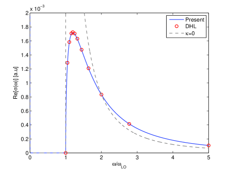
Figure III.1: Optical absorption coefficient for Fröhlich polaron at $T=0$ for $\alpha=0.01.$ The full blue line represent the present result, the dashed gray line ($\kappa=0$) would be the result obtained without screening cit:SelsBrosensTruncate and the red circles (DHL) is a perturbative result by Devreese et al. cit:DHL .

Fig. (III.1) clearly shows the effect of dynamical screening on the optical absorption. When the effect of the induced electric field is ignored, i.e. $\kappa=0,$ the absorption becomes more singular near the absorption threshold and the high frequency absorption is slightly reduced. As implied by the polaron-f-sum rule cit:DLVRsumrule , the total absorption for $\omega>\omega_{LO}$ is smaller when dynamical screening is taken into account. In agreement with the polaron-f-sum rule, the reduction of the total absorption beyond threshold reduces the relative change in the mass by a factor 2. For comparison Fig. (III.1) also shows a weak coupling result due to Devreese et al. cit:DHL (hereafter referred to as DHL). Their result is perturbative in $\alpha$ and thus becomes exact for $\alpha\rightarrow 0.$ For $\alpha=0.01$ their result is indistinguishable from the present result, which implies the present truncation scheme correctly predicts the weak coupling optical absorption. For $\alpha=1$ we show the absorption spectrum in Fig. (III.2).

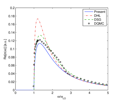
Figure III.2: Optical absorption coefficient for Fröhlich polaron at $T=0$ for $\alpha=1.$ The full blue line represent the present result, the dashed red line (DHL) is a perturbative result by Devreese et al. cit:DHL . Furthermore, the dashed green line (DSG) is a variational result due to Devreese et al. cit:DSG and the circles (DQMC) show a numerical result due to Mishchenko et al. cit:DQMC . DSG and DQMC data copied with permission of the authors from cit:KliminDevreese .

At this point there is a clear distinction between the present approach and the DHL result. We therefore compare the result with the absorption obtained from a diagrammatic quantum Monte Carlo calculation cit:DQMC which should give numerically exact answers for all $\alpha.$ Although the present result is distinguishable from the Monte Carlo calculation, it is clearly more accurate than the perturbative result of DHL. Moreover, the present result is remarkably close to the nonperturbative method presented in Ref. cit:DSG . The method, due to Devreese et al. cit:DSG , employs the impedance function approximation of FHIP cit:FHIP1962 . The method is thus nonperturbative in the sense that no expansion in the coupling constant is assumed.

IV Conclusion

In conclusion we have presented the first order self-energy correction to the linear response coefficients of polaronic systems within the truncated phase space approach developed by the present authors in cit:SelsBrosensTruncate . It is shown how the change of the self-energy due to the external perturbation induces an internal field. The first order correction thus comes in terms of a dynamic polarizability $\kappa.$ It is shown that the relative change in the effective mass is only half of the change without dynamical screening. Consequently, a significant amount of spectral weight must be moved to the central peak. Explicit expressions for the conductivity of the Fröhlich polaron are obtained. The results are shown to be in agreement with standard weak coupling theories for $\alpha\ll 1.$ Comparing with numerically exact data, we found that the present approach significantly improves on the standard weak coupling perturbation theory and extends the validity up to $\alpha\approx 1.$

- (1) D. Sels and F. Brosens, Phys. Rev. E 89, 012124 (2014)
- (2) D. Sels and F. Brosens, Phys. Rev. E 88, 042101 (2013)
- (3) H. Fröhlich, H., Proc. R. Soc. Lond. A160, 230 (1937).
- (4) H. Fröhlich, H. Pelzer, S. Zienau, Phil. Mag. 41, 221 (1950).
- (5) H. Fröhlich, Adv. Phys. 3, 325 (1954).
- (6) R. Feynman, R. Hellwarth, C. Iddings, and P. Platzman, Phys. Rev. 127, 1004 (1962).
- (7) L. P. Kadanoff, Phys. Rev. 130, 4 (1963).
- (8) V. F. Los’, Theor. and Math. Phys. 60, 703 (1984).
- (9) J. T. Devreese, L. Lemmens, and J. Van Royen, Phys. Rev. B 15, 1212–1214 (1977)
- (10) A. S. Alexandrov and J. T. Devreese, Advances in Polaron Physics, Springer-Verlag Berlin Heidelberg (2010).
- (11) J. T. Devreese, Lectures on Fröhlich Polarons from 3D to 0D, arXiv:1012.4576
- (12) J.T. Devreese, W. Huybrechts, and L. Lemmens, Phys. Stat.Sol. (b) 48, 77 (1971)
- (13) J.T. Devreese, J. De Sitter, and M. Goovaerts, Phys. Rev. B 5, 2367 (1972).
- (14) A.S. Mishchenko, N. Nagaosa, N. V. Prokof’ev, A. Sakamoto, and B. V. Svistunov, Phys. Rev. Lett. 91, 236401 (2003).
- (15) J.T. Devreese and S. Klimin, private communication