Abstract

The conditional autoregressive model is a routinely used statistical model for areal data that arise from, for instances, epidemiological, socio-economic or ecological studies. Various multivariate conditional autoregressive models have also been extensively studied in the literature and it has been shown that extending from the univariate case to the multivariate case is not trivial. The difficulties lie in many aspects, including validity, interpretability, flexibility and computational feasibility of the model. In this paper, we approach the multivariate modeling from an element-based perspective instead of the traditional vector-based perspective. We focus on the joint adjacency structure of elements and discuss graphical structures for both the spatial and non-spatial domains. We assume that the graph for the spatial domain is generally known and fixed while the graph for the non-spatial domain can be unknown and random. We propose a very general specification for the multivariate conditional modeling and then focus on three special cases, which are linked to well known models in the literature. Bayesian inference for parameter learning and graph learning is provided for the focused cases, and finally, an example with public health data is illustrated.

Keywords: Areal data; Disease mapping; Graphical model; G-Wishart distribution; Markov random field; Reversible jump.

1 Introduction

Areal data, sometimes called lattice data, are usually represented by an undirected graph where each vertex represents an areal unit and each edge represents a neighboring relationship. A finite set of random variables on an undirected graph, where each vertex is a random variable, is called a Markov random field if it has the Markov property. Hence, the Markov random field models are often used for the areal data. The univariate conditional autoregressive (CAR) model, originated from Besag (1974), is a Gaussian Markov random field model, for which the joint distribution is multivariate Gaussian. Let $\bm{u}=(u_{1},\ldots,u_{I})^{T}$ be a vector of random variables on $I$ areal units (i.e. $I$ vertices). The zero-centered conditional autoregressive model specifies full conditional Gaussian distributions

$$u_{i}\mid u_{-i}\sim\mbox{N}\left(\sum_{i^{\prime}\neq i}b_{ii^{\prime}}u_{i^{\prime}},\tau_{i}^{2}\right),~{}~{}~{}i=1,\ldots,I,$$

where $u_{-i}$ is the collection of $u_{i^{\prime}}$ for $i^{\prime}\neq i$. The resulting joint distribution, derived using Brook’s lemma, has a density function as follows,

$$f(\bm{u}\mid\bm{T}_{\textsc{CAR}},\bm{B}_{\textsc{CAR}})\propto\mbox{exp}\left\{-\frac{1}{2}\bm{u}^{T}\bm{T}^{-1}_{\textsc{CAR}}(\bm{I}-\bm{B}_{\textsc{CAR}})\bm{u}\right\},$$

where $\bm{I}$ is an identity matrix; $\bm{B}_{\textsc{CAR}}$ is an $I\times I$ matrix whose off-diagonal entries are $b_{ii^{\prime}}$ and diagonal entries are zeros, and $\bm{T}_{\textsc{CAR}}=\operatorname{diag}\{\tau_{1}^{2},\ldots,\tau_{I}^{2}\}$. The joint distribution is multivariate Gaussian if and only if $\bm{T}^{-1}_{\textsc{CAR}}(\bm{I}-\bm{B}_{\textsc{CAR}})$ is symmetric and positive definite. A further parameterization on $\bm{B}_{\textsc{CAR}}$ and $\bm{T}_{\textsc{CAR}}$ is needed to reduce the number of parameters in the model. Consider a so-called adjacency matrix $\bm{C}_{\textsc{CAR}}$ for the undirected graph, where the $ii^{\prime}$th entry $C_{ii^{\prime}}=1$ if unit $i$ and unit $i^{\prime}$ are neighbors (denoted as $i\sim i^{\prime}$) and $C_{ii^{\prime}}=0$ otherwise. One popular parameterization is to let $b_{ii^{\prime}}=\rho C_{ii^{\prime}}/C_{i+}$ and $\tau_{i}^{2}=\sigma^{2}/C_{i+}$, where $C_{i+}$ is the $i$th row sum of $\bm{C}_{\textsc{CAR}}$, representing the total number of neighbors of unit $i$. Let $\bm{D}_{\textsc{CAR}}=\operatorname{diag}\{C_{1+},\ldots,C_{I+}\}$. When $\rho$ is strictly between the smallest and largest eigenvalues of $\bm{D}_{\textsc{CAR}}^{-1/2}\bm{C}_{\textsc{CAR}}\bm{D}_{\textsc{CAR}}^{-1/2}$, or sufficiently, when $|\rho|<1$, and $\sigma^{2}>0$, the joint distribution of $\bm{u}$ is a zero-mean multivariate Gaussian distribution: $\bm{u}\sim N\{{\bf 0},\sigma^{2}(\bm{D}_{\textsc{CAR}}-\rho\bm{C}_{\textsc{CAR}})^{-1}\}$. This is called the proper conditional autoregressive model in the literature. When $\rho=1$, it is called the intrinsic conditional autoregressive model which is an improper distribution due to the singular covariance matrix.

Turning to the multivariate case, consider $J$ responses (e.g. multiple diseases) on $I$ areal units. Let $\bm{U}$ be an $I\times J$ matrix-variate where the $ij$th entry $u_{ij}$ is a random variable for the $i$th areal unit and $j$th response. Each column of $\bm{U}$ is an areal vector for a single response and hence can be modeled by the univariate conditional autoregressive model. However, a multivariate model is desired for the matrix-variate $\bm{U}$ in order to simultaneously model the dependence across responses. Initially proposed by Mardia (1988), the multivariate conditional autoregressive model specifies full conditional distributions on row vectors of $\bm{U}$. Let $\bm{u}_{i}$ be the $i$th row vector of $\bm{U}$. Following Besag (1974), specify

$$\bm{u}_{i}\mid\bm{u}_{-i}\sim\mbox{N}\left(\sum_{i^{\prime}\neq i}\bm{B}_{ii^{\prime}}\bm{u}_{i^{\prime}},\bm{\Sigma}_{i}\right),~{}~{}~{}i=1,\ldots,I,$$ (1)

where $\bm{B}_{ii^{\prime}}$ and $\bm{\Sigma}_{i}$ are $J\times J$ matrices needing a further parameterization. To make the joint distribution for $\mathop{\operator@font vec}\nolimits(\bm{U}^{T})$ a multivariate Gaussian, $\bm{B}_{ii^{\prime}}$ and $\bm{\Sigma}_{i}$ must satisfy certain conditions (Mardia, 1988). Gelfand & Vounatsou (2003) showed a convenient parameterization, $\bm{B}_{ii^{\prime}}=(\rho C_{ii^{\prime}}/C_{i+})\bm{I}_{J}$ and $\bm{\Sigma}_{i}=\bm{\Sigma}/C_{i+}$. When $|\rho|<1$ and $\bm{\Sigma}$ is positive definite, $\mathop{\operator@font vec}\nolimits(\bm{U}^{T})$ has a zero-mean multivariate Gaussian distribution: $\mathop{\operator@font vec}\nolimits(\bm{U}^{T})\sim N\{{\bf 0},(\bm{D}_{\textsc{CAR}}-\rho\bm{C}_{\textsc{CAR}})^{-1}\otimes\bm{\Sigma}\}$. It is clear that this multivariate specification is a Kronecker product formula where $(\bm{D}_{\textsc{CAR}}-\rho\bm{C}_{\textsc{CAR}})^{-1}$ models the covariance structure across rows of $\bm{U}$ (spatial domain) and $\bm{\Sigma}$ models the covariance structure across columns of $\bm{U}$ (response domain). From the modeling perspective, Mardia’s specification has a difficulty with parameterization. It is usually difficult to have a meaningful parameterization for $\bm{B}_{ii^{\prime}}$ and $\bm{\Sigma}_{i}$ unless one pursues a simple formulation. It is arguable that the Mardia’s specification presents a conflict, where the between vector variation is specified through an inverse covariance matrix, but the within vector variation is specified through a covariance matrix. It seems more intuitive to either work with the joint covariance or the joint inverse covariance directly. Notice that most multivariate spatial models for point reference data focus on the joint covariance structure. In this paper, we focus on the joint inverse covariance structure of elements in the multivariate areal data. In particular, we consider the joint adjacency structure of the lattice based on graphical structures of both the spatial domain and the response domain. We build a framework for graph based multivariate conditional autoregressive models and discuss parameterizations under this framework. The advantage is that this framework is very general and we demonstrate it through multiple case examples. Furthermore, we allow graph learning for multiple responses in such models, which is potentially useful for many modern applications.

We shall point out other recent work on multivariate conditional autoregressive models. Kim et al. (2001) and Jin et al. (2005) proposed conditional autoregressive models for bivariate areal data. Multivariate models were considered by Gelfand & Vounatsou (2003), Jin et al. (2007), MacNab (2011, 2016), Martinez-Beneito (2013); Martinez-Beneito et al. (2017) among many others. MacNab (2018) reviewed some recent developments on multivariate Gaussian Markov random field models. We will show that some of the earlier work can be reconstructed in our proposed framework and some can be extended to graphical models. The paper is organized as follows. Section 2 presents the general framework and three special parameterizations. Section 3 presents a real data example using the proposed models. Section 5 contains further discussions and remarks. Technical details are given in the appendix.

2 Graph-based Multivariate Conditional Autoregressive Models

2.1 General framework

Instead of specifying full conditional distributions on vectors like (1), we approach this problem from an element-based perspective. Following Besag (1974), specify full conditional distributions for each element $u_{ij}$ in the matrix-variate $\bm{U}$ as follows,

$$u_{ij}\mid u_{-\{ij\}}\sim\mbox{N}\left(\sum_{\{i^{\prime}j^{\prime}\}\neq\{ij\}}b_{\{ij\},\{i^{\prime}j^{\prime}\}}u_{i^{\prime}j^{\prime}},\tau_{ij}^{2}\right),~{}~{}~{}i=1,\ldots,I~{}\mbox{and}~{}j=1,\ldots,J,$$

where $\{i^{\prime}j^{\prime}\}\neq\{ij\}$ means either $i^{\prime}\neq i$ or $j^{\prime}\neq j$. In fact, here we consider a lattice consisting of all elements in $\bm{U}$. Using Brook’s lemma, the resulting joint distribution for $\mathop{\operator@font vec}\nolimits(\bm{U})$ is

$$f(\mathop{\operator@font vec}\nolimits(\bm{U})\mid\bm{B},\bm{T})\propto\exp\left\{-\frac{1}{2}\mathop{\operator@font vec}\nolimits(\bm{U})^{T}\bm{T}^{-1}(\bm{I}-\bm{B})\mathop{\operator@font vec}\nolimits(\bm{U})\right\},$$

where $\bm{I}$ is an $IJ\times IJ$ identity matrix, $\bm{T}=\operatorname{diag}\{\tau_{11}^{2},\ldots,\tau_{I1}^{2},\ldots,\tau_{1J}^{2},\ldots,\tau_{IJ}^{2}\}$ and $\bm{B}$ can be expressed block-wisely,

$$\bm{B}=\begin{pmatrix}\bm{B}_{11}&\cdots&\bm{B}_{1J}\\ \vdots&\ddots&\vdots\\ \bm{B}_{J1}&\cdots&\bm{B}_{JJ}\end{pmatrix}\mbox{~{}~{}~{}where~{}~{}~{}}\bm{B}_{jj^{\prime}}=\begin{pmatrix}b_{\{1j\},\{1j^{\prime}\}}&\cdots&b_{\{1j\},\{Ij^{\prime}\}}\\ \vdots&\ddots&\vdots\\ b_{\{Ij\},\{1j^{\prime}\}}&\cdots&b_{\{Ij\},\{Ij^{\prime}\}}\end{pmatrix},$$

and the diagonal elements $b_{\{ij\},\{ij\}}$ are zeros. The joint distribution for $\mathop{\operator@font vec}\nolimits(\bm{U})$ is multivariate Gaussian if and only if $\bm{T}^{-1}(\bm{I}-\bm{B})$ is symmetric and positive definite. It is desired that $\bm{B}$ and $\bm{T}$ are further parameterized to reduce the number of parameters in the model. We denote this general model $\textsc{MCAR}(\bm{B},\bm{T})$ for later use.

Consider the adjacency structure of the undirected graph for the lattice of $\bm{U}$. In the univariate situation, the adjacency structure is determined by those geographical locations. Two areal units are connected by an edge if they are neighbors geographically. However, it is not obvious which elements should be neighbors in $\bm{U}$. Consider that the $J$ responses can be connected through an undirected graph. Let $\bm{C}^{(s)}$ be the adjacency matrix for all $I$ areal units and $\bm{C}^{(r)}$ be the adjacency matrix for all $J$ responses. Both the spatial graph and the response graph are then uniquely determined by $\bm{C}^{(s)}$ and $\bm{C}^{(r)}$, respectively. Let $\bm{C}$ be the joint adjacency matrix for the lattice of $\bm{U}$. A general construction of $\bm{C}$ can be made through $\bm{C}^{(s)}$ and $\bm{C}^{(r)}$,

$$\bm{C}=\bm{C}^{(r)}\otimes\bm{C}^{(s)}+\bm{C}^{(r)}\otimes\bm{I}_{I}+\bm{I}_{J}\otimes\bm{C}^{(s)}.$$ (2)

This construction connects $u_{ij}$ with $u_{i^{\prime}\sim i,j}$, $u_{i,j^{\prime}\sim j}$ and $u_{i^{\prime}\sim i,j^{\prime}\sim j}$, meaning its spatial neighbor, response neighbor and interaction neighbor, respectively. One may add edges for secondary neighbors or drop edges in a specific modeling. For example, some reduced constructions would be: (i) $\bm{C}=\bm{I}_{J}\otimes\bm{C}^{(s)}$ (independent conditional autoregressive models, no dependence between responses); (ii) $\bm{C}=\bm{C}^{(r)}\otimes\bm{I}_{I}$ (independent multivariate variables, no spatial dependence); (iii) $\bm{C}=\bm{C}^{(r)}\otimes\bm{I}_{I}+\bm{I}_{J}\otimes\bm{C}^{(s)}$ (drop edges for interaction neighbors $u_{i^{\prime}\sim i,j^{\prime}\sim j}$).

Let $C_{\{ij\},\{i^{\prime}j^{\prime}\}}$ denote entries in $\bm{C}$, analogous to the block-wise notation $b_{\{ij\},\{i^{\prime}j^{\prime}\}}$ for $\bm{B}$. Let $d_{j}^{(r)}$ be the $j$th row sum in $\bm{C}^{(r)}$ and $d_{i}^{(s)}$ be the $i$th row sum in $\bm{C}^{(s)}$. Then the $ij$th row sum in $\bm{C}$ is $d_{ij}=d_{j}^{(r)}d_{i}^{(s)}+d_{j}^{(r)}+d_{i}^{(s)}$. Let $\bm{D}^{(r)}=\operatorname{diag}\{d_{1}^{(r)},\ldots,d_{J}^{(r)}\}$, $\bm{D}^{(s)}=\operatorname{diag}\{d_{1}^{(s)},\ldots,d_{I}^{(s)}\}$ and $\bm{D}=\operatorname{diag}\{d_{11},\ldots,d_{I1},\ldots,d_{1J},\ldots,d_{IJ}\}$. With the adjacency constructions and notations, we then explore further parameterization on $\bm{B}$ and $\bm{T}$ in the following subsections, and specifically, we discuss three specifications made from this general framework, all of which are linked to well known models in the literature.

2.2 Model 1: nonseparable multifold specification

Kim et al. (2001) developed a twofold conditional autoregressive model for bivariate areal data ($J=2$), using different linkage parameters for different types of neighbors. Those linkage parameters, in their work, are called smoothing and bridging parameters, representing the strength of information sharing. If we extend their specification to an arbitrary $J$, we can parameterize $\bm{B}$ and $\bm{T}$ in the following way (assuming $i\neq i^{\prime}$ and $j\neq j^{\prime}$):

$$b_{\{ij\},\{i^{\prime}j\}}=\frac{\lambda_{j}}{d_{ij}}C_{\{ij\},\{i^{\prime}j\}},~{}~{}~{}b_{\{ij\},\{ij^{\prime}\}}=\frac{\psi_{jj^{\prime}}}{d_{ij}}\sqrt{\frac{\delta_{j}}{\delta_{j^{\prime}}}}C_{\{ij\},\{ij^{\prime}\}},$$

$$b_{\{ij\},\{i^{\prime}j^{\prime}\}}=\frac{\phi_{jj^{\prime}}}{d_{ij}}\sqrt{\frac{\delta_{j}}{\delta_{j^{\prime}}}}C_{\{ij\},\{i^{\prime}j^{\prime}\}},~{}~{}~{}\tau_{ij}^{2}=\frac{\delta_{j}}{d_{ij}},$$

where $\lambda_{j}$, $\psi_{jj^{\prime}}$ and $\phi_{jj^{\prime}}$ are linkage parameters and $\delta_{j}$ are variance components. Linkage parameters are for three types of neighbor: $u_{i^{\prime}\sim i,j}$, $u_{i,j^{\prime}\sim j}$ and $u_{i^{\prime}\sim i,j^{\prime}\sim j}$. Having this specification, the conditional mean of $u_{ij}$ essentially is

$$\mbox{E}(u_{ij}\mid u_{-\{ij\}})=\frac{1}{d_{ij}}\left(\lambda_{j}\sum_{i^{\prime}\sim i}u_{i^{\prime}j}+\psi_{jj^{\prime}}\sum_{j^{\prime}\sim j}\sqrt{\frac{\delta_{j}}{\delta_{j^{\prime}}}}u_{ij^{\prime}}+\phi_{jj^{\prime}}\sum_{i^{\prime}\sim i}\sum_{j^{\prime}\sim j}\sqrt{\frac{\delta_{j}}{\delta_{j^{\prime}}}}u_{i^{\prime}j^{\prime}}\right),$$

which is a weighted average of all its neighbors in $\bm{C}$. This specification generalizes Kim et al. (2001)’ twofold model and hence could be called a multifold specification. It can be shown that, for this parameterization, the joint precision matrix is

$$\bm{T}^{-1}(\bm{I}-\bm{B}) = (\bm{\Delta}^{-\frac{1}{2}}\otimes\bm{I}_{I})\left\{\bm{D}-\bm{\Lambda}\otimes\bm{C}^{(s)}\right.$$ (3)

$$\left.-(\bm{\Psi}\circ\bm{C}^{(r)})\otimes\bm{I}_{I}-(\bm{\Phi}\circ\bm{C}^{(r)})\otimes\bm{C}^{(s)}\right\}(\bm{\Delta}^{-\frac{1}{2}}\otimes\bm{I}_{I}),$$

where $\bm{\Delta}=\operatorname{diag}\{\delta_{1},\ldots,\delta_{J}\}$, $\bm{\Lambda}=\operatorname{diag}\{\lambda_{1},\ldots,\lambda_{J}\}$, $\bm{\Psi}$ and $\bm{\Phi}$ are $J\times J$ symmetric matrices with entries $\psi_{jj^{\prime}}$ and $\phi_{jj^{\prime}}$, respectively, and the operator $\circ$ means an element-wise product. A derivation of (3) is given in Appendix 1. Note that only nonzero entries of $\bm{\Psi}$ and $\bm{\Phi}$ are parameters in the model, the number of which depends on $\bm{C}^{(r)}$.

In order to make (3) positive definite, constraints on $\lambda_{j}$, $\psi_{jj^{\prime}}$ and $\phi_{jj^{\prime}}$ are needed, assuming that $\delta_{j}>0$. In general, it is difficult to find a sufficient and necessary condition for the positive definiteness of (3). Kim et al. (2001)’s solution to this problem was a sufficient condition: $\mbox{max}\{|\lambda_{j}|,|\psi_{jj^{\prime}}|,|\phi_{jj^{\prime}}|;\forall j,j^{\prime}\}<1$, under which the matrix (3) is diagonally dominant and hence is positive definite. Though their proof was under $J=2$, it is true for any $J$ by the same arguments. The advantage of this condition is that it is simple and implementable. However, this is not a necessary condition meaning that it is impossible to reach all possible positive definite structures for the model under such a condition. In a Bayesian model, priors on parameters $\lambda_{j}$, $\psi_{jj^{\prime}}$ and $\phi_{jj^{\prime}}$ can be chosen based on their actual constraints. In our case, a uniform prior $\mbox{Unif}(-1,1)$ is adequate for these linkage parameters. Priors on the variance components $\delta_{j}$ can be weakly-informative inverse-gamma priors $\mbox{IG}(a_{j},b_{j})$. Inference and computation under this model are given in Appendix 2.

2.3 Model 2: separable specification with homogeneous spatial smoothing

Gelfand & Vounatsou (2003)’s Kronecker-product model is a convenient parameterization of Mardia (1988)’s model. In our framework, this specification can be obtained and extended by having the following parameterization for $\bm{B}$ and $\bm{T}$ (assuming $i\neq i^{\prime}$ and $j\neq j^{\prime}$):

$$b_{\{ij\},\{i^{\prime}j\}}=\frac{\rho}{d_{i}^{(s)}}C_{\{ij\},\{i^{\prime}j\}},~{}~{}~{}b_{\{ij\},\{ij^{\prime}\}}=-\frac{\omega_{jj^{\prime}}}{\omega_{jj}}C_{\{ij\},\{ij^{\prime}\}},$$

$$b_{\{ij\},\{i^{\prime}j^{\prime}\}}=\frac{\rho\omega_{jj^{\prime}}}{d_{i}^{(s)}\omega_{jj}}C_{\{ij\},\{i^{\prime}j^{\prime}\}},~{}~{}~{}\tau_{ij}^{2}=\frac{1}{d_{i}^{(s)}\omega_{jj}},$$

where $\rho$ and $\omega_{jj^{\prime}}$ are linkage parameters, and $1/\omega_{jj}$ are variance components. This parameterization does not seem straightforward, but is much clearer in the form of conditional mean:

$$\mbox{E}\left(u_{ij}-\frac{\rho}{d_{i}^{(s)}}\sum_{i^{\prime}\sim i}u_{i^{\prime}j}~{}\Bigg{|}~{}u_{-\{ij\}}\right)=-\sum_{j^{\prime}\sim j}\frac{\omega_{jj^{\prime}}}{\omega_{jj}}\left(u_{ij^{\prime}}-\frac{\rho}{d_{i}^{(s)}}\sum_{i^{\prime}\sim i}u_{i^{\prime}j^{\prime}}\right).$$ (4)

Note that for a single response, the univariate conditional autoregressive model specifies $\mbox{E}(u_{i}|u_{-i})=\rho\sum_{i^{\prime}\sim i}u_{i^{\prime}}/d_{i}^{(s)}$. In the multivariate setting, $\rho\sum_{i^{\prime}\sim i}u_{i^{\prime}j}/d_{i}^{(s)}$ is no longer the conditional mean for $u_{ij}\mid u_{-\{ij\}}$ and their conditional difference is regressed on other differences through $\omega_{jj^{\prime}}$. This parameterization yields the joint precision matrix

$$\bm{T}^{-1}(\bm{I}-\bm{B}) = \left\{\bm{\Omega}\circ(\bm{I}_{J}+\bm{C}^{(r)})\right\}\otimes(\bm{D}^{(s)}-\rho\bm{C}^{(s)})$$ (5)

$$= \bm{\Omega}_{\bm{C}^{(r)}}\otimes(\bm{D}^{(s)}-\rho\bm{C}^{(s)}),$$

where $\bm{\Omega}$ is a symmetric $J\times J$ matrix with entries $\omega_{jj^{\prime}}$. A derivation of (5) is given in Appendix 1. The linkage parameter $\rho$ is interpreted as a spatial smoothing parameter and $\bm{\Omega}$ controls the dependence across $J$ responses. It is noteworthy that only nonzero entries in $\bm{\Omega}$ are parameters in the model and we denote $\bm{\Omega}_{\bm{C}^{(r)}}=\bm{\Omega}\circ(\bm{I}_{J}+\bm{C}^{(r)})$ for simplicity. The notation $\bm{\Omega}_{\bm{C}^{(r)}}$, commonly used in graphical models, means the precision matrix restricted by graph $\bm{C}^{(r)}$. The model (5) is a natural extension of Gelfand & Vounatsou (2003)’s model. When $\bm{C}^{(r)}$ is the complete graph (any two vertices are connected), $\bm{\Omega}_{\bm{C}^{(r)}}$ is free of zero entries. Then let $\bm{\Sigma}=\bm{\Omega}^{-1}$ and (5) is equivalent to Gelfand & Vounatsou (2003)’s specification. We call this a completely separable specification because the Kronecker product completely separates the spatial domain and the response domain. This complete separation is often not desirable because it makes the spatial smoothing common for all $j$. We call this homogeneous spatial smoothing because the linkage $\rho$ is the same for any $i$ and $i^{\prime}$ which distinguishes Model 2 from Model 3 in the next subsection.

The joint precision matrix (5) is positive definite if $|\rho|<1$ and $\bm{\Omega}_{\bm{C}^{(r)}}$ is positive definite. Let $M^{+}({\bm{C}^{(r)}})$ be the cone of symmetric positive definite matrices restricted by $\bm{C}^{(r)}$ and then $\bm{\Omega}_{\bm{C}^{(r)}}\in M^{+}({\bm{C}^{(r)}})$. In a Bayesian model, a widely used prior on $\bm{\Omega}_{\bm{C}^{(r)}}$ is the G-Wishart distribution (Atay-Kayis & Massam, 2005; Letac & Massam, 2007). The G-Wishart distribution is a conjugate family for the precision matrix of a Gaussian graphical model, whose density function is given by

$$p(\bm{\Omega}_{\bm{C}^{(r)}}\mid b,\bm{V})=I_{\bm{C}^{(r)}}(b,\bm{V})^{-1}\left|\bm{\Omega}_{\bm{C}^{(r)}}\right|^{\frac{b-2}{2}}\mbox{exp}\left\{-\frac{1}{2}\mbox{tr}(\bm{V}\bm{\Omega}_{\bm{C}^{(r)}})\right\}1_{\bm{\Omega}_{\bm{C}^{(r)}}\in M^{+}({\bm{C}^{(r)}})},$$

where $b>2$ is the number of degrees of freedom; $\bm{V}$ is the scale matrix and $I_{\bm{C}^{(r)}}(\cdot)$ is the normalizing constant. It is practically attractive because of its conjugacy. That said, for a prior distribution $\mbox{GWis}(b,\bm{V})$ and a given sample covariance matrix $\bm{S}$ of sample size $n$, the posterior distribution of $\bm{\Omega}_{\bm{C}^{(r)}}$ is $\mbox{GWis}(b+n,\bm{V}+\bm{S})$. Inference and computation under this model are given in Appendix 2.

2.4 Model 3: separable specification with heterogenous spatial smoothing

Dobra et al. (2011) introduced a multivariate lattice model by giving Kronecker product G-Wishart priors to the matrix-variate $\bm{U}$. In our framework, $\bm{B}$ and $\bm{T}$ can be parameterized in the following way (assuming $i\neq i^{\prime}$ and $j\neq j^{\prime}$):

$$b_{\{ij\},\{i^{\prime}j\}}=-\frac{\omega_{ii^{\prime}}^{(s)}}{\omega_{ii}^{(s)}}C_{\{ij\},\{i^{\prime}j\}},~{}~{}~{}b_{\{ij\},\{ij^{\prime}\}}=-\frac{\omega_{jj^{\prime}}^{(r)}}{\omega_{jj}^{(r)}}C_{\{ij\},\{ij^{\prime}\}},$$

$$b_{\{ij\},\{i^{\prime}j^{\prime}\}}=-\frac{\omega_{ii^{\prime}}^{(s)}\omega_{jj^{\prime}}^{(r)}}{\omega_{ii}^{(s)}\omega_{jj}^{(r)}}C_{\{ij\},\{i^{\prime}j^{\prime}\}},~{}~{}~{}\tau_{ij}^{2}=\frac{1}{\omega_{ii}^{(s)}\omega_{jj}^{(r)}},$$

which is equivalent to the version of conditional mean

$$\mbox{E}\left(u_{ij}-\frac{1}{\omega_{ii}^{(s)}}\sum_{i^{\prime}\sim i}\omega_{ii^{\prime}}^{(s)}u_{i^{\prime}j}~{}\Bigg{|}~{}u_{-\{ij\}}\right)=-\sum_{j^{\prime}\sim j}\frac{\omega_{jj^{\prime}}}{\omega_{jj}}\left(u_{ij^{\prime}}-\frac{1}{\omega_{ii}^{(s)}}\sum_{i^{\prime}\sim i}\omega_{ii^{\prime}}^{(s)}u_{i^{\prime}j^{\prime}}\right).$$ (6)

Comparing (6) with (4), instead of a homogeneous spatial smoothing with $\rho$, it has a heterogeneous specification with $\omega_{ii^{\prime}}^{(s)}$. This is hence more flexible in the spatial domain. The resulting joint precision matrix is

$$\bm{T}^{-1}(\bm{I}-\bm{B}) = \left\{\bm{\Omega}^{(r)}\circ(\bm{I}_{J}+\bm{C}^{(r)})\right\}\otimes\left\{\bm{\Omega}^{(s)}\circ(\bm{I}_{I}+\bm{C}^{(s)})\right\}$$ (7)

$$= \bm{\Omega}_{\bm{C}^{(r)}}\otimes\bm{\Omega}_{\bm{C}^{(s)}},$$

where $\bm{\Omega}^{(r)}$ is a symmetric $J\times J$ matrix with entries $\omega^{(r)}_{jj^{\prime}}$ and $\bm{\Omega}^{(s)}$ is a symmetric $I\times I$ matrix with entries $\omega^{(s)}_{ii^{\prime}}$. A derivation of (7) is given in Appendix 1. We again use $\bm{\Omega}_{\bm{C}^{(r)}}$ and $\bm{\Omega}_{\bm{C}^{(s)}}$ for simplicity. In model (5), the spatial part is the conventional conditional autoregressive model while in model (7), it is modeled by a more flexible one $\bm{\Omega}_{\bm{C}^{(s)}}$.

The precision matrix (7) is positive definite if both $\bm{\Omega}_{\bm{C}^{(r)}}$ and $\bm{\Omega}_{\bm{C}^{(s)}}$ are positive definite. In a Bayesian model, both can have G-Wishart priors. The specification has an obvious problem of identification: $\bm{\Omega}_{\bm{C}^{(r)}}\otimes\bm{\Omega}_{\bm{C}^{(s)}}=z\bm{\Omega}_{\bm{C}^{(r)}}\otimes(1/z)\bm{\Omega}_{\bm{C}^{(s)}}$, where $z$ is an arbitrary constant scalar. Following Wang & West (2009), one can impose a constraint $\bm{\Omega}_{\bm{C}^{(r)},11}=1$ and add an auxiliary variable $z$. Then specify a joint prior on $(z,z\bm{\Omega}_{\bm{C}^{(r)}})$:

$$p(z,z\bm{\Omega}_{\bm{C}^{(r)}}\mid b^{(r)},\bm{V}^{(r)})\propto p_{GWis}(z\bm{\Omega}_{\bm{C}^{(r)}}\mid b^{(r)},\bm{V}^{(r)})\cdot 1,$$ (8)

where $p_{GWis}(\cdot)$ is the density of G-Wishart distribution. Transform this joint density to $(z,\bm{\Omega}_{\bm{C}^{(r)}})$ and we obtain the desired joint prior. There is no additional constraint imposed on $\bm{\Omega}_{\bm{C}^{(s)}}$ and let $\bm{\Omega}_{\bm{C}^{(s)}}\sim\mbox{GWis}(b^{(s)},\bm{V}^{(s)})$. Inference and computation under this model are given in Appendix 2.

2.5 Priors for the graph

The two types of graphs used in this modeling framework should be treated differently. On one hand, the spatial graph should be treated known and fixed because the geographical locations and their neighboring structure is fixed in most scenarios. On the other hand, the response graph should be treated unknown because we often know little about the relationship between multiple responses. In the literature of Gaussian graphical model determination, usually the unknown graph is assumed random and a prior on the graph is assigned. The Markov chain Monte Carlo (MCMC) sampling scheme, such as the reversible jump MCMC (Green, 1995), is often used to sample graphs from the posterior distribution. In this paper, we adopt and slightly modify existing MCMC algorithms for the graph determination (Wang & Li, 2012; Dobra et al., 2011), with computational details given in Appendix 2, for each aforementioned model. For the prior choice of $\bm{C}^{(r)}$, consider

$$P(\bm{C}^{(r)})\propto B(a+\mbox{size}(\bm{C}^{(r)}),b+m-\mbox{size}(\bm{C}^{(r)}))/B(a,b),$$ (9)

where $B(\cdot,\cdot)$ is the beta function, $m$ is the total number of possible edges $J\choose 2$, $\mbox{size}(\bm{C}^{(r)})\in\{0,1,\ldots,m\}$, and $a$ and $b$ are given hyperparameters. More details about this prior can be found in Scott & Berger (2006) and Scott & Carvalho (2009). The following prior is often used as well (Dobra et al., 2011):

$$P(\bm{C}^{(r)})\propto\pi^{\mbox{size}(\bm{C}^{(r)})}(1-\pi)^{m-\mbox{size}(\bm{C}^{(r)})},$$ (10)

where $\pi\in(0,1)$ is a given hyperparameter. Sparser graphs can be favored by choosing a small value for $\pi$. The prior (9) can be obtained by integrating $\pi$ out with a hyperprior $\mbox{Beta}(a,b)$ on $\pi$.

3 An Application

We illustrate the proposed models with a real example of disease mapping. It is known that smoking is linked with multiple diseases in the population, of which leading diseases include lung diseases and heart diseases. The dataset under consideration here includes six variables, among which four variables are related to the smoke exposure and the other two are diseases. Obtained from the 2011 Missouri County Level Survey, the four smoke exposure variables are: Current Cigarette Smoking, Current Smokeless Tobacco Use, Current Other Tobacco Use, Exposure to Secondhand Smoke. Data are binary responses to the survey questionnaires (Yes or No), aggregated to each county level. The other two variables, obtained from the Surveillance, Epidemiology and End Results (SEER) program, are the Lung Cancer Mortality and the Heart Diseases Mortality, both of which are counts for each county within a specified time period. To summarize, we have $I=115$ counties and $J=6$ response variables. Let $n_{i1},\ldots,n_{i4}$ be the numbers of respondents in the survey and let $E_{i5}$ and $E_{i6}$ be the age-adjusted expected mortality for the two diseases. Then, the proportions $y_{ij}/n_{ij},~{}j=1,\ldots,4$ are empirical estimates of the prevalences of the survey variables, and the proportions $y_{ij}/E_{ij},~{}j=5,6$ are standardized mortality ratios of the diseases.

Consider a Bayesian hierarchical model for $y_{ij}$. We use the binomial-logit model and the Poisson-lognormal model (Banerjee et al., 2004) for $y_{i,1-4}$ and $y_{i,5-6}$, respectively, i.e.

$$y_{ij}\sim\mbox{Bin}(n_{ij},p_{ij}),~{}~{}~{}\mbox{logit}(p_{ij})=\beta_{j}+u_{ij},~{}~{}~{}i=1,\ldots,115\mbox{ and }j=1,\dots,4;$$

$$y_{ij}\sim\mbox{Poi}(E_{ij}\eta_{ij}),~{}~{}~{}\mbox{log}(\eta_{ij})=\beta_{j}+u_{ij},~{}~{}~{}i=1,\ldots,115\mbox{ and }j=5,6.$$

For simplicity, we do not consider other covariates in this example. The primary interest here is to model the random effects $u_{ij}$, which are expected to be correlated in both the spatial domain and the response domain. To complete the model specification, specify a weakly-informative normal prior for the intercepts $\beta_{j}$ and a multivariate conditional autoregressive model $\textsc{MCAR}(\bm{B},\bm{T})$ for the random effects $\bm{U}=\{u_{ij}\}$. We apply the three proposed versions of $\textsc{MCAR}(\bm{B},\bm{T})$ here. Hyperparameters for prior distributions are specified as follows. For the graph, noticing that the choice of $\pi$ in (10) can influence the posterior inference, we consider the prior (10) with both $\pi=0.2$ in favor of a sparse graph and $\pi=0.5$ as no preference. All other priors are chosen to be only weakly-informative and have little impact on the posterior inference. In Model 1, we specify hyperparameters in the inverse gamma prior as $a_{j}=b_{j}=0.5$. In Model 2, we specify hyperparameters in the G-Wishart prior as $b=3$ and $\bm{V}=\bm{I}$. In Model 3, we specify hyperparameters in the two G-Wishart priors as $b=3,\bm{V}=\bm{I},b^{(s)}=24$ and $\bm{V}^{(s)}=(b^{(s)}-2)(\bm{D}-0.95\bm{C})^{-1}$, which implies a prior mode at a proper conditional autoregressive model. For each model, we perform the Markov chain Monte Carlo for 150,000 iterations with a burn-in size of 50,000. Posterior results are based on the remaining samples. Figure 1 shows the convergence of the log-joint-posterior and notice that they all converge quickly.

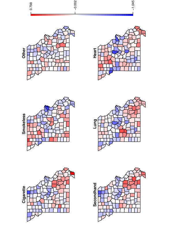
Figure 2: Posterior means of spatial random effects $u_{ij}$ under Model 1.

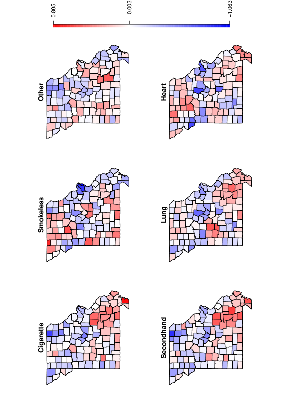
Figure 3: Posterior means of spatial random effects $u_{ij}$ under Model 2.

Table 1 shows the posterior edge inclusion probabilities for the response graph $\bm{C}^{(r)}$. First, all three models seem to agree on the link between Cigarette Smoking and Secondhand Smoke Exposure, as well as the link between Lung Diseases Mortality and Heart Diseases Mortality. There is a moderate agreement on the links between Secondhand Smoke Exposure and Lung Diseases Mortality, and between Cigarette Smoking and Lung Diseases Mortality. In general, Model 1 tends to be a sparser graph, which is possibly due to the diagonal dominance condition. Model 2 is the simplest model as reflected by its pD, the effective number of parameters, but has the largest DIC. Model 3 is the most flexible model among the three, and the inferred graph tends to be denser than the other two. It is as expected that its pD is larger but the overall criterion DIC is much smaller than the other two. Second, the edge inclusion probabilities are in general higher when $\pi=0.5$, as expected, but it has little material impact on the final inferred graph. The DIC has little change with different $\pi$ values. Lastly, Figures 1 - 3 show the maps of spatial random effects $u_{ij}$ for the three models, respectively, and for a problem of disease mapping, this is often the eventual output for practitioners.

4 Simulation

To validate the proposed algorithms, we perform a simulation study on a $7\times 7$ regular grid ($I=49$ area units) with $J=4$ response variables. Consider the true response graph with two edges $C^{(r)}_{13}$ and $C^{(r)}_{24}$. In this simulation study, we do not consider the scenario with misspecified models, and therefore, data are generated under each of the three models and the correct model is then used for inference. The parameter settings are given as follows. For Model 1, $\lambda_{j}=0.95$, $\phi_{jj^{\prime}}=\psi_{jj^{\prime}}=0.9$, $\delta_{j}=1$ and $\beta_{j}=1$. For Model 2, $\rho=0.9$, $\omega_{jj}=4$, $\omega_{13}=\omega_{24}=-3.2$ and $\beta_{j}=1$. For Model 3, parameters are the same as Model 2 but $\bm{\Omega}_{\bm{C}^{(s)}}$ is generated from $\mbox{GWis}(10,8(\bm{D}-0.9\bm{C})^{-1})$. We repeat the simulation and inference process for $L=50$ times and for each time, the MCMC iteration number is 5,000. We consider three measures for validating and comparing the three algorithms. The first measure is the mean inclusion probability matrix with standard deviations. We call the second measure the error rate of mis-identified edges. If we use 0.5 as the threshold for identifying an edge in the graph, for each replication, we obtain an inferred graph and then compare with the true graph to record a proportion of wrong edges/non-edges. The error rate is the average proportion of $L$ replications. The third measure is the mean absolute error (MAE) of random effects in the model,

$$\mbox{MAE}=\frac{1}{L}\frac{1}{J}\frac{1}{I}\sum_{l}\sum_{j}\sum_{i}\left|\frac{\hat{u}_{ijl}-u_{ijl}}{u_{ijl}}\right|$$

where $u_{ijl}$ is the true value and $\hat{u}_{ijl}$ is the posterior mean.

Simulation results are given in Table 2. For all three models, the algorithms can correctly identify the true edges. The algorithm for Model 1 appears to be unstable as the standard deviation is large and tends to underestimate inclusion probabilities, while the algorithm for Model 3 tends to overestimate inclusion probabilities for non-edges. The algorithm for Model 2 presents the smallest error rate and MAE. Note that this simulation study validates the proposed algorithms under correct model specifications and hence the result cannot imply that Model 2 is the best model for a real dataset. In fact, as shown in the data analysis, Model 2 is the simplest specification and is the least preferred model in that case according to DIC.

5 Further Discussion

In this paper, we proposed a modeling framework for multivariate areal data from a graphical model perspective. We rebuilt three well known models in our framework and developed Bayesian inference tools for the proposed models. It is our perspective that this framework is very general and can contain other models that are beyond the cases discussed in the paper. For example, Jin et al. (2007) specified a co-regionalized areal data model, in which their Case 3 is a very general specification. We show that this specification can be reproduced and extended in our framework. Consider the Cholesky decomposition $\bm{\Sigma}=\bm{A}\bm{A}^{T}$. Jin et al. (2007)’s Case 3 specification of the joint covariance matrix is $(\bm{A}\otimes\bm{I}_{I})(\bm{I}_{J}\otimes\bm{D}^{(s)}-\bm{\Phi}\otimes\bm{C}^{(s)})^{-1}(\bm{A}\otimes\bm{I}_{I})^{T}$ whose inverse is then

$$(\bm{A}\bm{A}^{T})^{-1}\otimes\bm{D}^{(s)}-(\bm{A}^{-1})^{T}\bm{\Phi}\bm{A}^{-1}\otimes\bm{C}^{(s)}$$ (11)

where $\bm{\Phi}$ is a symmetric $J\times J$ matrix. Let $\bm{\Omega}=\bm{\Sigma}^{-1}=(\bm{A}\bm{A}^{T})^{-1}$ and $\bm{Q}=(\bm{A}^{-1})^{T}\bm{\Phi}\bm{A}^{-1}$. Obviously it is one-to-one from $(\bm{A},\bm{\Phi})$ to $(\bm{\Omega},\bm{Q})$. Specification (11) is hence equivalent to

$$\bm{\Omega}\otimes\bm{D}^{(s)}-\bm{Q}\otimes\bm{C}^{(s)},$$ (12)

where $\bm{Q}$ is a symmetric $J\times J$ matrix with entries $q_{jj^{\prime}}$. To reproduce this specification in our framework, parameterize $\bm{B}$ and $\bm{T}$ as follows (assuming $i\neq i^{\prime}$ and $j\neq j^{\prime}$):

$$b_{\{ij\},\{i^{\prime}j\}}=\frac{q_{jj}}{d_{i}^{(s)}\omega_{jj}}C_{\{ij\},\{i^{\prime}j\}},~{}~{}~{}b_{\{ij\},\{ij^{\prime}\}}=-\frac{\omega_{jj^{\prime}}}{\omega_{jj}}C_{\{ij\},\{ij^{\prime}\}},$$

$$b_{\{ij\},\{i^{\prime}j^{\prime}\}}=\frac{q_{jj^{\prime}}}{d_{i}^{(s)}\omega_{jj}}C_{\{ij\},\{i^{\prime}j^{\prime}\}},~{}~{}~{}\tau_{ij}^{2}=\frac{1}{d_{i}^{(s)}\omega_{jj}}.$$

This parameterization leads to the joint precision matrix

$$\bm{T}^{-1}(\bm{I}-\bm{B}) = \left\{\bm{\Omega}\circ(\bm{I}_{J}+\bm{C}^{(r)})\right\}\otimes\bm{D}^{(s)}-\left\{\bm{Q}\circ(\bm{I}_{J}+\bm{C}^{(r)})\right\}\otimes\bm{C}^{(s)}$$ (13)

$$= \bm{\Omega}_{\bm{C}^{(r)}}\otimes\bm{D}^{(s)}-\bm{Q}_{\bm{C}^{(r)}}\otimes\bm{C}^{(s)}.$$

The expression (13) reduces to (12) which is equivalent to Jin et al. (2007)’s (11) when $\bm{C}^{(r)}$ is a complete graph. A derivation of (13) is given in Appendix 1. The validity of this model relies on the positive definiteness of (13). Jin et al. (2007) showed that it is positive definite if $\bm{\Omega}$ is positive definite and eigenvalues of $\bm{\Phi}=\bm{A}^{T}\bm{Q}\bm{A}$ are between $1/\xi_{\mbox{min}}$ and $1/\xi_{\mbox{max}}$, reciprocals of the smallest and largest eigenvalues of $\bm{D}^{(s)-1/2}\bm{C}^{(s)}\bm{D}^{(s)-1/2}$, which are known constants. The graphical version (13) must also satisfy this condition, that is, $1/\xi_{\mbox{min}}\leq\lambda(\bm{\Omega}_{\bm{C}^{(r)}}^{-1}\bm{Q}_{\bm{C}^{(r)}})\leq 1/\xi_{\mbox{max}}$, where $\lambda(\bm{M})$ is any eigenvalue of $\bm{M}$. Considering that both $\bm{\Omega}_{\bm{C}^{(r)}}$ and $\bm{Q}_{\bm{C}^{(r)}}$ are restricted by the underlying graph, the eigenvalue condition is not easy to implement in computations. This matter is worth investigating in the future.

In general, flexible models are desired for modeling multivariate areal data because overly simplistic models may misspecify the true underlying covariance structure. However, there is almost always a trade-off between the simplicity and the flexibility of a model. It is probably reasonable to allow certain flexibilities for specific purposes, such as in this paper, for learning a graphical relationship between multiple responses. It is usually the practitioner’s choice whether a more flexible but complicated model is needed for the problem at hand, especially when the performance improvement is negligible.

Appendix 1: Derivations

Derivation of equation (3)

With the parameterization in Model 1, we have $\bm{T}=\bm{D}^{-1}(\bm{\Delta}\otimes\bm{I}_{I})$ and

$$\bm{B}=(\bm{\Delta}^{\frac{1}{2}}\otimes\bm{I}_{I})\bm{D}^{-1}\left\{\bm{\Lambda}\otimes\bm{C}^{(s)}+(\bm{\Psi}\circ\bm{C}^{(r)})\otimes\bm{I}_{I}+(\bm{\Phi}\circ\bm{C}^{(r)})\otimes\bm{C}^{(s)}\right\}(\bm{\Delta}^{-\frac{1}{2}}\otimes\bm{I}_{I}).$$

Then immediately we have expression (3) for $\bm{T}^{-1}(\bm{I}-\bm{B})$.

Derivation of equation (5)

With the parameterization in Model 2, we have $\bm{T}=\left(\operatorname{diag}(\bm{\Omega})\otimes\bm{D}^{(s)}\right)^{-1}$ and

$$\bm{B}=\rho\bm{I}_{J}\otimes\bm{D}^{(s)-1}\bm{C}^{(s)}-\left(\operatorname{diag}(\bm{\Omega})^{-1}\bm{\Omega}\circ\bm{C}^{(r)}\right)\otimes\bm{I}_{I}+\rho\left(\operatorname{diag}(\bm{\Omega})^{-1}\bm{\Omega}\circ\bm{C}^{(r)}\right)\otimes\bm{D}^{(s)-1}\bm{C}^{(s)}.$$

Then

$$\bm{T}^{-1}(\bm{I}-\bm{B}) = \operatorname{diag}(\bm{\Omega})\otimes\bm{D}^{(s)}-\rho\operatorname{diag}(\bm{\Omega})\otimes\bm{C}^{(s)}+(\bm{\Omega}\circ\bm{C}^{(r)})\otimes\bm{D}^{(s)}-\rho(\bm{\Omega}\circ\bm{C}^{(r)})\otimes\bm{C}^{(s)}$$

$$= \left\{\bm{\Omega}\circ(\bm{I}_{J}+\bm{C}^{(r)})\right\}\otimes\bm{D}^{(s)}-\left\{\bm{\Omega}\circ(\bm{I}_{J}+\bm{C}^{(r)})\right\}\otimes\rho\bm{C}^{(s)}$$

$$= \left\{\bm{\Omega}\circ(\bm{I}_{J}+\bm{C}^{(r)})\right\}\otimes(\bm{D}^{(s)}-\rho\bm{C}^{(s)}),$$

which is expression (5).

Derivation of equation (7)

With the parameterization in Model 3, we have $\bm{T}=\left(\operatorname{diag}(\bm{\Omega}^{(r)})\otimes\operatorname{diag}(\bm{\Omega}^{(s)})\right)^{-1}$ and

$$\bm{B} = -\bm{I}_{J}\otimes\left(\operatorname{diag}(\bm{\Omega}^{(s)})^{-1}\bm{\Omega}^{(s)}\circ\bm{C}^{(s)}\right)-\left(\operatorname{diag}(\bm{\Omega}^{(r)})^{-1}\bm{\Omega}^{(r)}\circ\bm{C}^{(r)}\right)\otimes\bm{I}_{I}$$

$$-\left(\operatorname{diag}(\bm{\Omega}^{(r)})^{-1}\bm{\Omega}^{(r)}\circ\bm{C}^{(r)}\right)\otimes\left(\operatorname{diag}(\bm{\Omega}^{(s)})^{-1}\bm{\Omega}^{(s)}\circ\bm{C}^{(s)}\right).$$

Then

$$\bm{T}^{-1}(\bm{I}-\bm{B}) = \operatorname{diag}(\bm{\Omega}^{(r)})\otimes\operatorname{diag}(\bm{\Omega}^{(s)})+\operatorname{diag}(\bm{\Omega}^{(r)})\otimes(\bm{\Omega}^{(s)}\circ\bm{C}^{(s)})$$

$$+(\bm{\Omega}^{(r)}\circ\bm{C}^{(r)})\otimes\operatorname{diag}(\bm{\Omega}^{(s)})+(\bm{\Omega}^{(r)}\circ\bm{C}^{(r)})\otimes(\bm{\Omega}^{(s)}\circ\bm{C}^{(s)})$$

$$= \left\{\bm{\Omega}^{(r)}\circ(\bm{I}_{J}+\bm{C}^{(r)})\right\}\otimes\left\{\bm{\Omega}^{(s)}\circ(\bm{I}_{I}+\bm{C}^{(s)})\right\},$$

which is expression (7).

Derivation of equation (13)

With the parameterization in Model 4, we have $\bm{T}=\left(\operatorname{diag}(\bm{\Omega})\otimes\bm{D}^{(s)}\right)^{-1}$ and

$$\bm{B} = \operatorname{diag}(\bm{\Omega})^{-1}\operatorname{diag}(\bm{Q})\otimes\bm{D}^{(s)-1}\bm{C}^{(s)}-\operatorname{diag}(\bm{\Omega})^{-1}\bm{\Omega}\circ\bm{C}^{(r)}\otimes\bm{I}_{I}$$

$$+\operatorname{diag}(\bm{\Omega})^{-1}\bm{Q}\circ\bm{C}^{(r)}\otimes\bm{D}^{(s)-1}\bm{C}^{(s)}.$$

Then

$$\bm{T}^{-1}(\bm{I}-\bm{B}) = \operatorname{diag}(\bm{\Omega})\otimes\bm{D}^{(s)}-\operatorname{diag}(\bm{Q})\otimes\bm{C}^{(s)}+\bm{\Omega}\circ\bm{C}^{(r)}\otimes\bm{D}^{(s)}-\bm{Q}\circ\bm{C}^{(r)}\otimes\bm{C}^{(s)}$$

$$= \left\{\bm{\Omega}\circ(\bm{I}_{J}+\bm{C}^{(r)})\right\}\otimes\bm{D}^{(s)}-\left\{\bm{Q}\circ(\bm{I}_{J}+\bm{C}^{(r)})\right\}\otimes\bm{C}^{(s)},$$

which is expression (13).

Appendix 2: Bayesian Computations

A hierarchical generalized linear model

For illustration, we now assume a full Bayesian hierarchical model and give computational details for this model. Assume binomial counts $y_{ij}/n_{ij}$ for $J$ responses and $I$ areal units. Specify a Bayesian model as follows, for $i=1,\ldots,I$ and $j=1,\dots,J$,

$$y_{ij}\mid p_{ij}\sim\mbox{Bin}(n_{ij},p_{ij}),~{}~{}~{}~{}~{}~{}~{}~{}\mbox{logit}(p_{ij})=\beta_{j}+u_{ij},$$

$$\beta_{j}\sim\mbox{N}(0,\tau_{0}^{2}),~{}~{}~{}~{}~{}~{}~{}~{}\bm{U}\mid\bm{B},\bm{T}\sim\textsc{MCAR}(\bm{B},\bm{T}),$$

where $\tau_{0}^{2}$ is a given constant, $\bm{U}$ is the matrix-variate of $u_{ij}$, and priors for $\bm{B}$ and $\bm{T}$ depend on the specific parameterization. This section is organized as follows: we first give details of updating effects parameters $\beta_{j}$ and $u_{ij}$, and then, separately for each model, details of updating parameters of MCAR and updating the random response graph $\bm{C}^{(r)}$.

Updating effects parameters

Our experience has shown that the convergence is poor if we directly update $\beta_{j}$ and $u_{ij}$. We apply the hierarchical centering technique (Gelfand et al., 1995) and block sampling. Let $\gamma_{ij}=\beta_{j}+u_{ij}$ and $\bm{\gamma}=\mathop{\operator@font vec}\nolimits[(\gamma_{ij})_{I\times J}]$ has a non-centered MCAR prior. We update $(\gamma_{ij},\beta_{j})$ instead of $(u_{ij},\beta_{j})$. The full conditional distribution of $\gamma_{ij}$ is

$$p(\gamma_{ij}\mid\cdot)\propto\frac{e^{y_{ij}\gamma_{ij}}}{(1+e^{\gamma_{ij}})^{n_{ij}}}\exp\left\{-\frac{1}{2\tau_{ij}^{2}}\left(\gamma_{ij}-\beta_{j}-\sum_{\{i^{\prime}j^{\prime}\}\neq\{ij\}}b_{\{ij\},\{i^{\prime}j^{\prime}\}}(\gamma_{i^{\prime}j^{\prime}}-\beta_{j^{\prime}})\right)\right\}.$$

We use Metropolis-Hastings algorithm to sample $\gamma_{ij}$ from this conditional density. We block sample $\bm{\beta}$ in the following way. For now denote $\bm{M}=\bm{T}^{-1}(\bm{I}-\bm{B})$, the joint precision matrix. Let $\bm{\gamma}^{*}=\bm{M}\bm{\gamma}$ and $\bm{\gamma}^{**}$ be a $J\times 1$ vector such that $\gamma^{**}_{1}$ is the sum of the first $I$ elements in $\bm{\gamma}^{*}$, $\gamma^{**}_{2}$ is the sum of the second $I$ elements in $\bm{\gamma}^{*}$ and so on. Partition $\bm{M}$ into $J\times J$ blocks and define

$$\bm{H}=\begin{pmatrix}{\bf 1}^{T}\bm{M}_{11}{\bf 1}&\cdots&{\bf 1}^{T}\bm{M}_{1J}{\bf 1}\\ \vdots&\ddots&\vdots\\ {\bf 1}^{T}\bm{M}_{J1}{\bf 1}&\cdots&{\bf 1}^{T}\bm{M}_{JJ}{\bf 1},\end{pmatrix}$$

where ${\bf 1}$ is the all-one vector. Then the full conditional distribution for the vector $\bm{\beta}$ is

$$(\bm{\beta}\mid\cdot)\sim\mbox{N}\left[(\bm{H}+1/\tau_{0}^{2}\bm{I})^{-1}\bm{\gamma}^{**},(\bm{H}+1/\tau_{0}^{2}\bm{I})^{-1}\right].$$

Model 1: updating $\delta_{j}$, $\lambda_{j}$, $\psi_{jj^{\prime}}$, $\phi_{jj^{\prime}}$ and $\bm{C}^{(r)}$

Given the current graph $\bm{C}^{(r)}$, parameters are updated through Gibbs sampling. Recall priors on these parameters: $\delta_{j}\sim\mbox{IG}(a_{j},b_{j})$ and $\lambda_{j},\psi_{jj^{\prime}},\phi_{jj^{\prime}}\sim\mbox{Unif}(-1,1)$. Let $\bm{u}_{j}$ be the $j$th column vector of $\bm{U}$, $j=1,\ldots,J$ and $\bm{D}_{j}$ be the $j$th diagonal block of $\bm{D}$. The full conditional distribution of $\delta_{j}$ is given by

$$p(\delta_{j}\mid\cdot)\propto\delta_{j}^{-\frac{I}{2}-a_{j}-1}\exp\left\{-\frac{1}{2\delta_{j}}\bm{u}_{j}^{T}(\bm{D}_{j}-\lambda_{j}\bm{C}^{(s)})\bm{u}_{j}+\sum_{j^{\prime}\sim j}\frac{1}{\sqrt{\delta_{j}\delta_{j^{\prime}}}}\bm{u}_{j}^{T}(\psi_{jj^{\prime}}\bm{I}_{I}+\phi_{jj^{\prime}}\bm{C}^{(s)})\bm{u}_{j^{\prime}}-\frac{b_{j}}{\delta_{j}}\right\}.$$

It can be shown that the transformed one $(\sqrt{1/\delta_{j}}\mid\cdot)$ is log-concave when $I+2a_{j}-1>0$. Thus, we use the adaptive rejection sampling to update $\delta_{j}$.

Let $\bm{W}$ be an $I\times J$ matrix, where $\mathop{\operator@font vec}\nolimits(\bm{W})=(\bm{\Delta}^{-1/2}\otimes\bm{I}_{I})\mathop{\operator@font vec}\nolimits(\bm{U})$ and $\bm{w}_{j}$ be the $j$th column vector of $\bm{W}$. Let $\bm{M}=\bm{D}-\bm{\Lambda}\otimes\bm{C}^{(s)}-(\bm{\Psi}\circ\bm{C}^{(r)})\otimes\bm{I}_{I}-(\bm{\Phi}\circ\bm{C}^{(r)})\otimes\bm{C}^{(s)}$ as in (3). Then $\lambda_{j}$, $\psi_{jj^{\prime}}$ and $\phi_{jj^{\prime}}$ are sequentially updated through following full conditional distributions,

$$p(\lambda_{j}\mid\cdot) \propto \left|\bm{M}(\lambda_{j})\right|^{\frac{1}{2}}\exp\left(\frac{1}{2}\lambda_{j}\bm{w}_{j}^{T}\bm{C}^{(s)}\bm{w}_{j}\right),$$

$$p(\psi_{jj^{\prime}}\mid\cdot) \propto \left|\bm{M}(\psi_{jj^{\prime}})\right|^{\frac{1}{2}}\exp\left(\psi_{jj^{\prime}}\bm{w}_{j}^{T}\bm{w}_{j^{\prime}}\right),$$

$$p(\phi_{jj^{\prime}}\mid\cdot) \propto \left|\bm{M}(\phi_{jj^{\prime}})\right|^{\frac{1}{2}}\exp\left(\phi_{jj^{\prime}}\bm{w}_{j}^{T}\bm{C}^{(s)}\bm{w}_{j^{\prime}}\right).$$

We use Metropolis-Hastings algorithm to update these parameters. Note that evaluating the sparse $|\bm{M}|$ could be computationally intensive. An efficient algorithm, usually based on the Cholesky decomposition, on sparse matrices is helpful.

The graph $\bm{C}^{(r)}$ is updated through a simple reversible jump MCMC algorithm. Propose a new graph $\bm{C}^{(r)*}$ by only adding or deleting one edge from $\bm{C}^{(r)}$. Without loss of generality, suppose that one edge $\{j0,k0\}$ is added to the new graph. Dimension has been changed by $2$ from $(\bm{C}^{(r)},\bm{\Psi},\bm{\Phi})$ to $(\bm{C}^{(r)*},\bm{\Psi}^{*},\bm{\Phi}^{*})$. Propose $u_{1}\sim U(-1,1)$ and $u_{2}\sim U(-1,1)$, and let $\psi^{*}_{j0,k0}=u_{1}$ and $\phi^{*}_{j0,k0}=u_{2}$. The Jacobian from $(\bm{\Psi},\bm{\Phi},u_{1},u_{2})$ to $(\bm{\Psi}^{*},\bm{\Phi}^{*})$ hence is $1$. Choose a Bernoulli jump proposal with odds $q(\bm{C}^{(r)*},\bm{C}^{(r)})/q(\bm{C}^{(r)},\bm{C}^{(r)*})=p(\bm{C}^{(r)})/p(\bm{C}^{(r)*})$ and systematically scan through the graph for updating. Accept the move from $\bm{C}^{(r)}$ to $\bm{C}^{(r)*}$ with probability $\min\{1,\alpha\}$ where

$$\alpha=\frac{|\bm{M}^{*}|^{\frac{1}{2}}}{|\bm{M}|^{\frac{1}{2}}}\exp\left\{-\frac{1}{2}\mathop{\operator@font vec}\nolimits(\bm{W})(\bm{M}^{*}-\bm{M})\mathop{\operator@font vec}\nolimits(\bm{W})\right\}.$$

Model 2: updating $\rho$, $\bm{\Omega}_{\bm{C}^{(r)}}$ and $\bm{C}^{(r)}$

Given the current graph $\bm{C}^{(r)}$, parameters are updated through Gibbs sampling. Recall priors on these parameters: $\rho\sim U(-1,1)$ and $\bm{\Omega}_{\bm{C}^{(r)}}\sim\mbox{GWis}(b,\bm{V})$. Use Metropolis-Hastings algorithm to update $\rho$. It can be shown that the full conditional distribution for $\rho$ is

$$p(\rho\mid\cdot)\propto\left|\bm{D}^{(s)}-\rho\bm{C}^{(s)}\right|^{\frac{J}{2}}\exp\left\{\frac{\rho}{2}\mathop{\operator@font vec}\nolimits(\bm{U})^{T}(\bm{\Omega}_{\bm{C}^{(r)}}\otimes\bm{C}^{(s)})\mathop{\operator@font vec}\nolimits(\bm{U})\right\}.$$

Let $\bm{W}_{1}$ be an $I\times J$ matrix, where $\mathop{\operator@font vec}\nolimits(\bm{W}_{1})=[\bm{I}_{J}\otimes(\bm{D}^{(s)}-\rho\bm{C}^{(s)})^{1/2}]\mathop{\operator@font vec}\nolimits(\bm{U})$ and $\bm{w}_{1,j}$ be the $j$th column vector of $\bm{W}_{1}$. Let $\bm{S}$ be an $J\times J$ matrix with $s_{jj^{\prime}}=\bm{w}_{1,j}^{T}\bm{w}_{1,j^{\prime}}$. Then the full conditional distribution of $\bm{\Omega}_{\bm{C}^{(r)}}$ is

$$p(\bm{\Omega}_{\bm{C}^{(r)}}\mid\cdot)\propto\left|\bm{\Omega}_{\bm{C}^{(r)}}\right|^{\frac{b+I-2}{2}}\exp\left[-\frac{1}{2}\operatorname{tr}\left\{\bm{\Omega}_{\bm{C}^{(r)}}(\bm{V}+\bm{S})\right\}\right]1_{\bm{\Omega}_{\bm{C}^{(r)}}\in M^{+}({\bm{C}^{(r)}})},$$

which is GWis($b+I,\bm{V}+\bm{S}$). For sampling from the G-Wishart distribution, we use the block Gibbs sampler, given the set of maximum cliques, introduced by Wang & Li (2012).

The graph $\bm{C}^{(r)}$ is updated using Wang & Li (2012)’s partial analytic structure algorithm (p. 188, Algorithm 2).

Model 3: updating $\bm{\Omega}_{\bm{C}^{(r)}}$, $\bm{\Omega}_{\bm{C}^{(s)}}$ and $\bm{C}^{(r)}$

Given the current graph $\bm{C}^{(r)}$, parameters are updated through Gibbs sampling. Recall that we impose a constraint and use a joint prior (8) on $(z,z\bm{\Omega}_{\bm{C}^{(r)}})$ and have $\bm{\Omega}_{\bm{C}^{(s)}}\sim\mbox{GWis}(b^{(s)},\bm{V}^{(s)})$. Let both $\bm{W}^{(r)}$ and $\bm{W}^{(s)}$ be $I\times J$ matrices, where $\mathop{\operator@font vec}\nolimits(\bm{W}^{(r)})=(\bm{I}_{J}\otimes\bm{\Omega}_{\bm{C}^{(s)}}^{1/2})\mathop{\operator@font vec}\nolimits(\bm{U})$ and $\mathop{\operator@font vec}\nolimits(\bm{W}^{(s)})=(\bm{\Omega}_{\bm{C}^{(r)}}^{1/2}\otimes\bm{I}_{I})\mathop{\operator@font vec}\nolimits(\bm{U})$. Let $\bm{w}_{j}^{(r)}$ be the $j$th column vector of $\bm{W}^{(r)}$ and $\bm{w}_{i}^{(s)}$ be the $i$th row vector of $\bm{W}^{(s)}$. Then let $\bm{S}^{(r)}$ be $J\times J$ with $s_{jj^{\prime}}^{(r)}=\bm{w}_{j}^{(r)T}\bm{w}_{j}^{(r)}$ and $\bm{S}^{(s)}$ be $I\times I$ with $s_{ii^{\prime}}^{(s)}=\bm{w}_{i}^{(s)T}\bm{w}_{i}^{(s)}$. With these notations, we have

$$(z\mid\cdot)\sim Ga(a_{z},b_{z}),$$

where $a_{z}=J(b-2)/2+\nu(\bm{C}^{(r)})$ and $b_{z}=\operatorname{tr}(\bm{\Omega}_{\bm{C}^{(r)}}\bm{V}^{(r)})/2$;

$$(\bm{\Omega}_{\bm{C}^{(r)}}\mid\cdot)\sim\mbox{GWis}(b^{(r)}+I,z\bm{V}^{(r)}+\bm{S}^{(r)})$$

and

$$(\bm{\Omega}_{\bm{C}^{(s)}}\mid\cdot)\sim\mbox{GWis}(b^{(s)}+J,\bm{V}^{(s)}+\bm{S}^{(s)}).$$

The graph $\bm{C}^{(r)}$ is updated using Wang & Li (2012)’s partial analytic structure algorithm (p. 188, Algorithm 2).

Model 1
	Cigarette	Smokeless	Other	Secondhand	Lung	Heart	pD	DIC
Cigarette		0	0.165	0.963	0.276	0	460.8	5766.5
Smokeless	0		0.181	0	0	0.002
Other	0.258	0		0.032	0.014	0.005
Secondhand	0.983	0	0.062		0.453	0
Lung	0.301	0	0.040	0.544		0.533
Heart	0.005	0	0.039	0.007	0.772		460.2	5765.0
Model 2
	Cigarette	Smokeless	Other	Secondhand	Lung	Heart	pD	DIC
Cigarette		0.213	0.919	1	0.756	0.373	445.1	5813.8
Smokeless	0.340		0.207	0.281	0.249	0.706
Other	0.872	0.316		0.390	0.346	0.898
Secondhand	1	0.527	0.475		0.732	0.343
Lung	0.584	0.407	0.412	0.871		1
Heart	0.352	0.942	0.838	0.400	1		447.2	5812.6
Model 3
	Cigarette	Smokeless	Other	Secondhand	Lung	Heart	pD	DIC
Cigarette		0.268	0.328	0.827	0.541	0.436	543.3	5630.4
Smokeless	0.249		0.417	0.692	0.515	0.726
Other	0.317	0.403		0.534	0.453	0.510
Secondhand	0.819	0.694	0.531		0.936	0.801
Lung	0.521	0.500	0.435	0.941		0.997
Heart	0.411	0.732	0.508	0.805	0.998		543.1	5629.2

Table 1: Data analysis: Posterior edge inclusion probabilities for the response graph and deviance information criterion for Models 1 - 3 respectively. Inclusion probabilities higher than 0.5 are in bold. The upper-right panel is for $\pi=0.2$ and the lower-left panel is for $\pi=0.5$.

Model 1
	Var 2	Var 3	Var 4	Error Rate	MAE
Var 1	0.128 (0.214)	0.664 (0.358)	0.088 (0.107)	0.15	3.167
Var 2		0.100 (0.148)	0.615 (0.352)
Var 3			0.087 (0.155)
Model 2
	Var 2	Var 3	Var 4	Error Rate	MAE
Var 1	0.211 (0.108)	1 (0)	0.200 (0.086)	0.02	2.153
Var 2		0.213 (0.134)	1 (0)
Var 3			0.199 (0.107)
Model 3
	Var 2	Var 3	Var 4	Error Rate	MAE
Var 1	0.246 (0.037)	0.961 (0.051)	0.292 (0.054)	0.07	2.218
Var 2		0.438 (0.092)	0.996 (0.008)
Var 3			0.426 (0.083)

Table 2: Simulation: Mean posterior edge inclusion probabilities (standard deviations in parentheses), error rates of mis-identified edges, and the mean absolute errors of random effects. True edges are in bold.

Figure 1: Convergence of the log joint posterior under the three models (first 50,000 iterations).

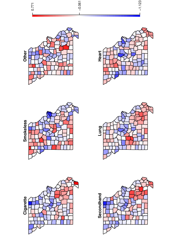
Figure 4: Posterior means of spatial random effects $u_{ij}$ under Model 3.

References

• (1)
• Atay-Kayis & Massam (2005) Atay-Kayis, A. & Massam, H. (2005), ‘A Monte Carlo method for computing the marginal likelihood in nondecomposable Gaussian graphical models’, Biometrika 92, 317–335.
• Banerjee et al. (2004) Banerjee, S., Gelfand, A. & Carlin, B. (2004), Hierarchical modeling and analysis for spatial data, CRC Press/Chapman & Hall.
• Besag (1974) Besag, J. (1974), ‘Spatial interaction and the statistical analysis of lattice systems’, Journal of the Royal Statistical Society. Series B 36, 192–236.
• Dobra et al. (2011) Dobra, A., A., L. & Rodriguez, A. (2011), ‘Bayesian inference for general Gaussian graphical models with applications to multivariate lattice data’, Journal of the American Statistical Association 106, 1418–1433.
• Gelfand et al. (1995) Gelfand, A., Sahu, S. & Carlin, B. (1995), ‘Efficient parameterizations for normal linear mixed models’, Biometrika 82, 479–488.