DGP braneworld with a bubble of nothing

Abstract

We construct exact solutions with the bubble of nothing in the Dvali-Gabadadze-Porrati braneworld model. The configuration with a single brane can be constructed, unlike in the Randall-Sundrum braneworld model. The geometry on the single brane looks like the Einstein-Rosen bridge. We also discuss the junction of multibranes. Surprisingly, even without any artificial matter fields on the branes such as three-dimensional tension of the codimension-two objects, two branes can be connected in certain configurations. We investigate solutions of multibranes too. The presence of solutions may indicate the semiclassical instability of the models.

I Introduction

The Dvali-Gabadadze-Porrati (DGP) braneworld is a model that may be able to explain the current acceleration of the Universe without introducing the cosmological constant DGP . Therein the four-dimensional universe is treated as a membrane with the induced gravity. The braneworld model is one of natural pictures of our Universe inspired by string theory, and the induced gravity is expected via the quantum correction into the matter fields on the brane loop . In the DGP models we often have the two type cosmological solutions Deffayet ; Gregory2006 , that is, the normal branch and the self-accelerating branch. The latter was expected to explain the current acceleration of the Universe. But, it was shown that the self-accelerating branch of the single brane model in the DGP braneworld is not compatible with observations Fang and also suffers from ghost instability Koyama:2005tx ; Izumi:2006ca (see Ref. Koyama for a review). However, there are still rooms for two branes models, which may realize the nonlinear massive gravity theory dRGT and/or bi-gravity theory bigravity (see Ref. deRham2014 for review) as an effective one Padilla , and the normal branch for single brane model.

In general, the spacetime with compact extra dimensions is semiclassically unstable if there is no fundamental fermion and/or supersymmetry. The spacetime decays to so-called Kaluza-Klein(KK) bubble-type spacetimes Witten . The bubble of nothing is nucleated via the quantum gravity effect. For the four-dimensional observers, the spacetime is incomplete at the surface on the bubble and the surface will expand with almost light velocity. The transition rate from the KK vacuum to the bubble depends on the size of the initial bubble. When the size is larger than the Planck scale, it is exponentially suppressed.

For the Randall-Sundrum braneworld model RS , the similar feature was reported Ida . In this paper, we discuss the same issue in the DGP braneworld context and focus on the construction of the braneworld model with the bubble of nothing. We will consider the normal branch on the brane although one may be interested in the self-accelerating branch. See Refs. Gregory2007 ; Izumi2007 for the related work (therein another decay channel was discussed, not bubble of nothing).

The remaining part of this paper is organized as follows. In Sec. II, we give the set-up for the DGP braneworld and the bulk spacetime. We also have a general remark. In Sec. III, we derive the junction condition on the brane for the current concrete case. In Sec. IV, the local embedding of branes in the bulk spacetime is discussed. In Sec. V, we derive the condition for connecting branes. In Sec. VI, we construct the spacetime globally for the single and multibranes cases. Finally we give the summary and discussion in Sec. VII.

II Setup

For simplicity, we consider the original DGP models described by the action DGP

$$S = 2M^{3}\int_{\rm bulk}d^{5}x{\sqrt{-g}}R$$ (1)

$$+2M^{3}\sum_{i}r_{i}\int_{{\rm{brane~{}}}i}d^{4}x{\sqrt{-q_{i}}}{}^{(4)}R(q_{i})$$

$$+\sum_{i}S_{{\rm{brane}}~{}i,~{}{\rm matter}}\ ,$$

where $R$ and ${}^{(4)}R$ are the five-dimensional Ricci scalar and the four-dimensional Ricci scalar of the branes. The index $i$ labels the branes. $g_{\mu\nu}$ and $q_{i\mu\nu}$ are the metric of the bulk and the branes. $M$ is the Planck scale in the five dimensions. $r_{i}$ has a length scale. Contrasted to the conventional higher dimensional theories, the five-dimensional effect will be crucial at a larger scale than $r_{i}$. $S_{{\rm{brane}}~{}i,~{}{\rm matter}}$ is the action for the matters localized on the branes.

Under the $Z_{2}$ symmetry, the junction condition is Israel

$$K_{i,\mu\nu}-K_{i}q_{i,\mu\nu}=r_{i}{}^{(4)}G_{\mu\nu}(q_{i})-\frac{1}{2M^{3}}T_{i,\mu\nu},$$ (2)

where $K_{i,\mu\nu}$ is the extrinsic curvature of the branes, ${}^{(4)}G_{\mu\nu}(q_{i})$ is the Einstein tensor for the metric $q_{i}$ and $T_{i,\mu\nu}$ is the energy-momentum tensor for the matters localized on the branes. The junction condition gives us the boundary condition for the bulk gravitational field equation, that is, the five-dimensional Einstein equation. The Greek indices $\{\mu,\nu,\ldots\}$ stand for the coordinate of the four-dimensional spacetime. Here, the unit normal vector $n^{\mu}$ required for the definition of the extrinsic curvature, $K_{i,\mu\nu}:=q_{i,\mu}{}^{\lambda}\nabla_{\lambda}n_{\nu}$, is oriented to the bulk.

For simplicity, we consider the vacuum cases, $T_{i,\mu\nu}=0$. Using the Gauss equation and the Weyl tensor, we have the equation on the brane as

$${}^{(4)}G_{\mu\nu} = r_{i}^{2}\Bigl{[}\frac{2}{3}{}^{(4)}R{}^{(4)}R_{\mu\nu}-{}^{(4)}R_{\mu\alpha}{}^{(4)}R_{\nu}^{~{}\alpha}$$

$$+\frac{1}{2}q_{\mu\nu}\Bigl{(}{}^{(4)}R_{\alpha\beta}{}^{(4)}R^{\alpha\beta}-\frac{1}{2}{}^{(4)}R^{2}\Bigr{)}\Bigr{]}-E_{\mu\nu},$$

where we have omitted $q_{i}$. $E_{\mu\nu}$ is the electric part of the Weyl tensor defined by $E_{\mu\nu}:={}^{(5)}C_{\mu\alpha\nu\beta}n^{\alpha}n^{\beta}$. This is the DGP version of the gravitational equation on branes for the Randall-Sundrum model SMS . Since the above is the quadratic equation with respect to the four-dimensional Ricci tensor, we can guess that there are two branches for the solutions. When $E_{\mu\nu}=0$ and ${}^{(4)}R_{\mu\nu}(q_{i})=\Lambda_{i}q_{i\mu\nu}$, we have $\Lambda_{i}(1-r_{i}^{2}\Lambda_{i}/3)=0$, and then $\Lambda_{i}=0$ (normal branch) or $\Lambda_{i}=3/r_{i}^{2}$ (self-accelerating branch).

The bulk spacetime follows the five-dimensional vacuum Einstein equation. As the simplest case, the bulk spacetime is just the five-dimensional Minkowski spacetime. In the canonical coordinate, the metric is $\eta_{5}=dy^{2}+\eta_{4}$, where $\eta_{4}$ is the metric of the four-dimensional Minkowski spacetime. The brane can be located at $y=$const. Indeed, this is a rather trivial case. This corresponds to the normal branch. Here we identify it with the DGP vacuum. The bulk metric is also written as the spherical Rindler coordinate $\eta_{5}=dz^{2}+z^{2}\gamma_{4}$, where $\gamma_{4}$ is the four-dimensional de Sitter solution with the positive cosmological constant of $3/r_{i}^{2}$. This belongs to the self-accelerating branch.

In this paper we suppose that the bulk spacetime is locally identical with the KK bubble spacetimes Witten

$$ds^{2}=f(r)d\chi^{2}+f(r)^{-1}dr^{2}+r^{2}\gamma_{ab}dx^{a}dx^{b},$$ (4)

where $f(r)=1\mp(r_{0}/r)^{2}$ and $\gamma_{ab}$ is the metric of the three-dimensional unit de Sitter spacetime. This spacetime is obtained through the double Wick rotation of the five-dimensional Schwarzschild spacetime. $f(r)$ with the negative (positive) sign is corresponding to the Schwarzschild spacetime with the positive (negative) mass. The Latin indices stand for the coordinate of the three-dimensional de Sitter spacetime.

For the KK bubble spacetime with the positive mass the periodicity $2\pi r_{0}$ for the coordinate $\chi$ makes the spacetime regular Witten , while in the KK bubble spacetime with the negative mass singularity always appears at $r=0$. For the moment, however, we do not care about the periodicity and the singularity, because we will use the KK bubble spacetime locally.

Here we have a comment on the simplest case, that is, the brane is located at $\chi=$const. In this case, the extrinsic curvature of the brane vanishes. Therefore,

$${}^{(4)}G_{\mu\nu}(q_{i})=\frac{1}{2M^{3}r_{i}}T_{i,\mu\nu}$$ (5)

must hold on the branes. The brane metric is

$$q_{i} = f(r)^{-1}dr^{2}+r^{2}\gamma_{ab}dx^{a}dx^{b}$$ (6)

$$= -r^{2}d\tau^{2}+f(r)^{-1}dr^{2}+r^{2}\left(\cosh\tau\right)^{2}d\Omega_{2}^{2},$$

where $d\Omega_{2}^{2}$ is the metric of the unit sphere. Then, the Einstein tensor on the brane is computed as

$${}^{(4)}G^{\mu}{}_{\nu}(q_{i})=\pm\frac{r_{0}^{2}}{r^{4}}(1,-3,1,1).$$ (7)

We must put the matter on the brane to be consistent with Eq. (5). This means that the energy-momentum tensor of the matter is proportional to the above. Then it is easy to see that the energy condition is broken. Therefore, if we suppose that the brane is at $\chi=$const, it is difficult to construct the physically acceptable braneworld model in the classical level. But, we may be able to realize it if one considers semiclassical treatment. This is beyond the scope of this paper.

III Local structure of DGP vacuum brane

In this section, we consider the local properties of the DGP braneworld such that the bulk spacetimes are locally given by the KK bubble spacetime of Eq. (4). For simplicity, we discuss vacuum branes. We write down the junction condition on the brane to have the equation that determines the location of the brane in the bulk.

Let us suppose that the brane is located at

$$\chi=\bar{\chi}_{i}(r).$$ (8)

The induced metric of the brane becomes

$$q_{i}=\alpha_{i}^{-2}dr^{2}+r^{2}\gamma_{ab}dx^{a}dx^{b},$$ (9)

where

$$\alpha_{i}:=(\bar{\chi}_{i}^{\prime 2}f+f^{-1})^{-1/2}>0.$$ (10)

The normal vector to the brane is

$$n_{i}=\alpha_{i}(d\chi-\bar{\chi}_{i}^{\prime}dr),$$ (11)

and then nonzero components of the extrinsic curvature of the brane are derived as

$$K^{r}{}_{r}=\alpha_{i}^{3}\Bigl{(}-\frac{3}{2}\bar{\chi}_{i}^{\prime}\frac{f^{\prime}}{f}-\frac{1}{2}\bar{\chi}_{i}^{\prime 3}ff^{\prime}-\bar{\chi}_{i}^{\prime\prime}\Bigr{)}$$ (12)

and

$$K^{a}{}_{b}=-\delta^{a}_{b}\frac{\bar{\chi}^{\prime}_{i}f}{r}.$$ (13)

From the induced metric, the nonzero components of the Ricci tensor are

$${}^{(4)}R^{r}{}_{r}=-3\frac{\alpha_{i}\alpha_{i}^{\prime}}{r}$$ (14)

and

$${}^{(4)}R^{a}{}_{b}=\frac{1}{r^{2}}\Bigl{[}2(1-\alpha_{i}^{2})-\alpha_{i}\alpha_{i}^{\prime}r\Bigr{]}\delta^{a}_{b}.$$ (15)

The Ricci scalar is

$${}^{(4)}R=\frac{6}{r^{2}}(1-\alpha_{i}^{2})-6\frac{\alpha_{i}\alpha_{i}^{\prime}}{r}.$$ (16)

It is ready to consider the junction condition. The $(a,b)$ components give us

$$\bar{\chi}_{i}^{\prime}=-\frac{r_{i}}{rf\alpha_{i}}(1-\alpha_{i}^{2}).$$ (17)

The $(r,r)$ component implies

$$\alpha_{i}^{3}\Bigl{(}\frac{3}{2}\bar{\chi}_{i}^{\prime}\frac{f^{\prime}}{f}+\frac{1}{2}\bar{\chi}_{i}^{\prime 2}ff^{\prime}+\bar{\chi}_{i}^{\prime\prime}\Bigr{)}$$

$$~{}~{}=r_{i}\Bigl{(}2\frac{\alpha_{i}\alpha_{i}^{\prime}}{r}+\frac{1}{r^{2}}(1-\alpha_{i}^{2})\Bigr{)}.$$ (18)

Note that this must be automatically satisfied when Eq. (17) holds, because they are related through the energy conservation law on the brane (for example, see Ref. Sasaki:1999mi ).

Together with the definition of $\alpha_{i}$, Eq. (17) gives us two solutions of $\alpha_{i}^{2}$ as

$$\alpha_{\pm,i}^{2}=\frac{-1+2(r_{i}/r)^{2}\pm{\sqrt{1-4(r_{0}/r)^{2}(r_{i}/r)^{2}}}}{2(r_{i}/r)^{2}}$$ (19)

for the positive mass case and

$$\alpha_{\pm,i}^{2}=\frac{-1+2(r_{i}/r)^{2}\pm{\sqrt{1+4(r_{0}/r)^{2}(r_{i}/r)^{2}}}}{2(r_{i}/r)^{2}}$$ (20)

for the negative mass case. In the limit $r\to\infty$, $\alpha_{+,i}$ approaches unity, while $\alpha_{-,i}$ does not have solutions. It means that the brane with $\alpha_{+,i}$ has asymptotically flat structure and thus the same asymptotic structure as that of the normal branch for the Minkowski bulk. On the other hand, the brane with $\alpha_{-,i}$ does not exist in the asymptotic region (although it could exist within certain finite $r$).

IV Trajectories of Single Brane

The number of solutions of $\alpha_{i}$ depends on the ratio of $r_{i}$ to $r_{0}$, which stems from requiring the presence of the square root in Eq. (19) or (20) and the positivity of $\alpha_{i}^{2}$. Below we will discuss the four cases (A)-(D), separately. Most of the trajectories of the brane in the ($r,\chi$) plane of the bulk terminate with the finite length or hit singularity. Only a trajectory for $r_{0}>r_{i}$ with the positive mass bulk goes to infinity, and thus, it would be geodesically complete. In this section, however, we do not care about the incompleteness of the trajectories and the singularities at the “edge” of the trajectories. The purpose in this section is deriving all possibilities of the local embedding of branes in the bulk spacetime with the metric of Eq. (4).

Hereafter we call the brane satisfying Eq. (19) or (20) for $\alpha_{+,i}$ ($\alpha_{-,i}$) the $+(-)$brane regardless of the positive or negative mass bulk.

IV.1 $r_{0}>r_{i}$ in positive mass bulk

The presence of the square root in Eq. (19) implies the condition $r\geq\sqrt{2r_{0}r_{i}}$ on the brane. $\alpha_{+,i}^{2}$ is positive only for $r\geq r_{*,i}:=\sqrt{r_{0}^{2}+r_{i}^{2}}$, while $\alpha_{-,i}^{2}$ always becomes negative. As a result, only $+$branes can exist in the range $r\geq r_{*,i}$.

The bulk (and the forbidden region) can be fixed by the direction of the unit normal vector $n_{\mu}$ as commented below Eq. (2). The unit normal vector $n_{\mu}$ is defined in Eq. (11) and the coefficient of $dr$ is $-\alpha_{i}{\bar{\chi}_{i}}^{\prime}$. From the definition of $\alpha_{i}$, i.e. Eq. (10), $\alpha_{i}$ must be smaller than unity. Combining this result with Eq. (17), it is easy to show the positivity of $-\alpha_{i}{\bar{\chi}_{i}}^{\prime}$. This means that the unit normal vector $n_{\mu}$ is pointing in the direction of increasing $r$, and thus, the region, where the coordinate $r$ is smaller than that on the brane with the same value of $\chi$, is forbidden and the remaining region becomes bulk (see Fig. 1). At the brane, the $Z_{2}$ symmetry is imposed.

By the integration of Eq. (17) with the boundary condition ${\bar{\chi}_{i}}(r_{*,i})=0$, we can obtain the trajectory of a $+$brane. However, the surface of $\chi={\bar{\chi}_{i}}(r)$, say $B_{p}$, is incomplete at $r=r_{*,i}$. This can be geodesically complete by reflecting with respect to the $\chi=0$ surface. The sum with the reflected surface $B_{m}$ of $\chi=-{\bar{\chi}_{i}}(r)$, $B=B_{p}\cup B_{m}$, is geodesically complete. The bulk spacetime is the region of $r\geq r_{0}$ removing the gray region as Fig. 1.

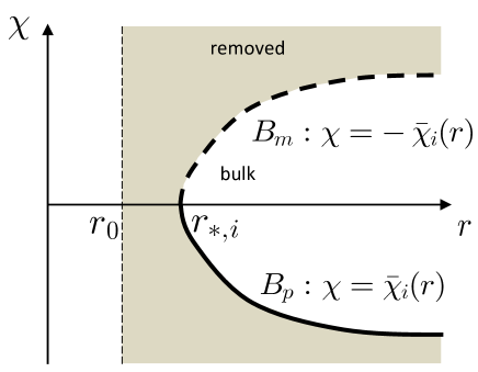
Figure 1: The location of the $+$brane in the ($\chi,r$) plane for $r_{0}>r_{i}$ and the positive mass bulk: The gray region is removed. This is only a regular solution with the single brane.

IV.2 $r_{0}<r_{i}$ in positive mass bulk

The presence of the square root in Eq. (19) constrains a lower limit of $r$ on the brane as $r\geq\sqrt{2r_{0}r_{i}}$. The positivity of $\alpha_{i}^{2}$ implies the upper limit $r_{*,i}={\sqrt{r_{0}^{2}+r_{i}^{2}}}$ only for $\alpha_{-,i}$. As a result, the $+$brane is embedded in the range $\sqrt{2r_{0}r_{i}}\leq r$ and the $-$brane is in the range $\sqrt{2r_{0}r_{i}}\leq r\leq r_{*,i}$. The argument of choosing the bulk region is the same as that in the previous case (see Fig. 2).

Unlike in the previous case, the $+$brane cannot be smoothly connected with its reflected image at the minimum value of $r$, ${\sqrt{2r_{0}r_{i}}}$. On the other hand, we can connect a $-$brane with its reflected image at $r=r_{*,i}$ in the same way of the previous case for $+$branes. Then, we have two possible solutions, on both branes of which geodesics are incomplete at $r=\sqrt{2r_{0}r_{i}}$ (see Figs. 2 and 3).

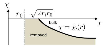
Figure 2: The location of the $+$brane in the ($\chi,r$) plane for $r_{0}<r_{i}$ and the positive mass bulk: The gray region is removed. The trajectory of the brane cannot be extended beyond $r=\sqrt{2r_{i}r_{0}}$

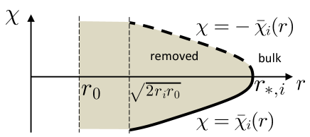
Figure 3: The location of the $-$brane in the ($\chi,r$) plane for $r_{0}<r_{i}$ and the positive mass bulk: The gray region is removed. The trajectory of the brane cannot be extended to the region of $r\leq\sqrt{2r_{i}r_{0}}$.

IV.3 $r_{0}<r_{i}$ in negative mass bulk

The square root in Eq. (20) is always positive, and thus, there are no restrictions for the range of $r$. The positivity of $\alpha_{i}^{2}$ gives the upper limit ${\bar{r}}_{*,i}:=\sqrt{r_{i}^{2}-r_{0}^{2}}$ only for the $-$brane. The bulk geometry has a singularity at $r=0$, and all single branes touch the singularity. As in the previous case, only the $-$brane can be connected with its reflected image at $r={\bar{r}}_{*,i}$.

The bulk region for the $\pm$branes is determined as shown in Figs. 4 and 5. Here we note that $\alpha_{+,i}^{2}$ always becomes larger than unity, which can be directly seen from Eq. (20), and this makes the sign of $(1-\alpha_{i}^{2})$ flipped. Then the position of bulk (Fig. 4) appears on the opposite side compared to the $-$brane case (Fig. 5).

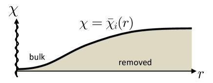
Figure 4: The location of the $+$brane in the ($\chi,r$) plane for the negative mass bulk: The gray region is removed. The trajectory of the brane hits the singularity at $r=0$.

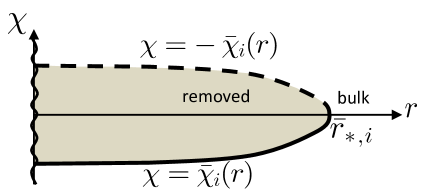
Figure 5: The location of the $-$brane in the ($\chi,r$) plane for the negative mass bulk: The gray region is removed. The trajectory of the brane hits the singularity at $r=0$.

IV.4 $r_{0}>r_{i}$ in negative mass bulk

For $+$branes, the discussion is the same as the previous one. Meanwhile, $\alpha_{-,i}^{2}$ always becomes negative, and thus, the $-$branes configuration does not exist. As a result, we have only a +branes configuration (see Fig. 4).

V Brane junction

In this section we shall discuss the possible brane junctions locally. In general, several branes intersect each other. At the junctions between branes, there is a restriction from field equations. In this section, we derive the equations for that.

We perform the integration of the equation for the vicinity of the junction point and then take the limit such that the integration domain goes to zero, as in the derivation of the junction condition for singular surfaces Israel . The integration of the $(a,b)$ component of the five-dimensional Einstein equation with respect to $\chi$ and $r$ gives

$$2M^{3}\int_{{\rm{bulk}}}d\chi dr\ G^{a}{}_{b}+2M^{3}\sum_{i}r_{i}\int_{{\rm{brane~{}}}i}dr\ {}^{(4)}G(q_{i})^{a}{}_{b}$$

$$\qquad\qquad\qquad-\frac{1}{2}\sum_{i}\int_{{\rm{brane~{}}}i}dr\ T_{i,}{}^{a}{}_{b}=0,$$ (21)

where $G^{a}{}_{b}$ is the five-dimensional Einstein tensor.

We classify the brane junctions into the four cases (Figs. 6-9). The first three, Figs. 6-8, are brane junctions in the positive mass bulk or $-$brane junctions in the negative mass bulk, where $\alpha_{i}$ is always smaller than unity. The last one, Fig. 9, describes the junctions of the $+$brane and the $-$brane in the negative mass bulk. We will look at them in detail.

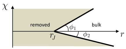
Figure 6: Case 1: Both branes approach the junction point $r=r_{J}$ from larger $r$.

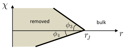
Figure 7: Case 2: Both branes approach the junction point $r=r_{J}$ from smaller $r$.

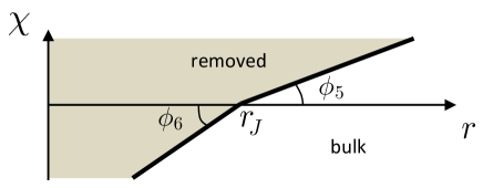
Figure 8: Case 3: One brane approaches the junction point $r=r_{J}$ from larger $r$, while another approaches the point $r=r_{J}$ from smaller $r$.

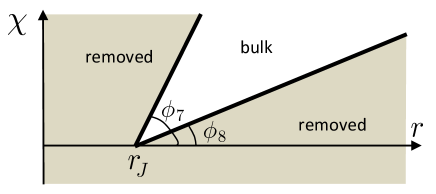
Figure 9: Case 4: The $-$brane is connected with a $+$brane for negative mass bulk.

V.1 Contribution from five-dimensional bulk gravity

The first term of Eq. (21) is evaluated through the contribution from the deficit angle $\phi$ as Israel:1976vc

$$\int dx^{2}\ G^{a}{}_{b}=-\frac{\phi}{2}\delta^{a}_{b}.$$ (22)

Therefore, what we have to do is only deriving the deficit angle. Then we compute it for each case.

(i) In case 1 (Fig. 6), both branes go to the direction of increasing $r$ from the junction point. Since the $Z_{2}$ symmetry is imposed across the branes, we can construct the bulk locally as Fig. 10. Then, the deficit angle is estimated at $2\pi-2\phi_{1}-2\phi_{2}$, where $\phi_{1}$ and $\phi_{2}$ are defined in Fig. 6 and they are taken to be a smaller value than $\pi$.

Using the bulk metric (4), the angle $\phi_{i}$ can be written as

$$\phi_{i} = \arctan\left|\frac{f^{1/2}}{f^{-1/2}}\frac{d\chi}{dr}\right|_{r=r_{J}}$$ (23)

$$= \left.\arctan\left(\frac{r_{i}}{r}\frac{1-\alpha_{i}^{2}}{\alpha_{i}}\right)\right|_{r=r_{J}},$$

where the branes are connected at $r=r_{J}$. Finally, from Eqs. (22) and (23), we see

$$\int d\chi dr\ G^{a}{}_{b}=\left.\sum_{i=1,2}\left[-\frac{\pi}{2}+\arctan\left(\frac{r_{i}}{r}\frac{1-\alpha_{i}^{2}}{\alpha_{i}}\right)\right]\right|_{r=r_{J}}\!\!\!\!\!\!\!\!\!\!\!\!\delta^{a}_{b}.$$

(24)

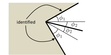
Figure 10: Gluing the mirror image due to $Z_{2}$-symmetry: The deficit angle becomes $2\pi-2\phi_{1}-2\phi_{2}$.

(ii) For case 2 (Fig. 7), both branes go to the direction of decreasing $r$ from the junction point. We can see the deficit angle becomes

$$2\pi-2(2\pi-\phi_{3}-\phi_{4})=-2\pi+2\phi_{3}+2\phi_{4}.$$ (25)

Then,

$$\int d\chi dr\ G^{a}{}_{b}=\left.\sum_{i=3,4}-\left[-\frac{\pi}{2}+\arctan\left(\frac{r_{i}}{r}\frac{1-\alpha_{i}^{2}}{\alpha_{i}}\right)\right]\right|_{r=r_{J}}\!\!\!\!\!\!\!\!\!\!\!\!\delta^{a}_{b}.$$

(iii) In case 3 (Fig. 8), the branes go to the opposite directions from each other with respect to $r$. In the same method the deficit angle becomes

$$2\pi-2(\pi+\phi_{5}-\phi_{6})=-2\phi_{5}+2\phi_{6},$$ (27)

and then

$$\int d\chi dr\ G^{a}{}_{b}=\left.\sum_{i=5,6}\epsilon_{i}\left[-\frac{\pi}{2}+\arctan\left(\frac{r_{i}}{r}\frac{1-\alpha_{i}^{2}}{\alpha_{i}}\right)\right]\right|_{r=r_{J}}\!\!\!\!\!\!\!\!\!\!\!\!\delta^{a}_{b},$$

where $\epsilon_{i}$ is unity for $\phi_{5}$ and $-1$ for $\phi_{6}$.

(iv) In case 4 (Fig. 9), both branes go to the direction of increasing both $\chi$ and $r$ from the junction point. Since $|{\bar{\chi}_{i}}^{\prime}|$ for the $-$brane is larger than that for the $+$brane, the $-$brane corresponds to one with the angle $\phi_{7}$ in Fig. 9. The deficit angle is $2\pi-2(\phi_{7}-\phi_{8})$. Here note that the sign of $(1-\alpha^{2})$ for the $+$brane is different from that in the previous cases, and then we compute as

$$\phi_{8} = \arctan\left|\frac{f^{1/2}}{f^{-1/2}}\frac{d\chi}{dr}\right|_{r=r_{J}}$$ (29)

$$= \left.-\arctan\left(\frac{r_{8}}{r}\frac{1-\alpha_{8}^{2}}{\alpha_{8}}\right)\right|_{r=r_{J}}.$$

For $\phi_{7}$, we can use Eq. (23), and then we arrive at Eq. (24).

V.2 Contribution from four-dimensional induced gravity

The second term of Eq. (21) comes from the discontinuity of the first derivative of the induced metric on the brane. Without loss of generality, we use the Gaussian normal coordinate $\bar{r}$ on the brane

$$d\bar{r}=\frac{dr}{\alpha_{i}}.$$ (30)

Then, the induced metric on the brane is written as

$$q_{i}=d{\bar{r}}^{2}+r^{2}(\bar{r})\gamma_{ab}dx^{a}dx^{b}.$$ (31)

On the brane, the extrinsic curvature $H_{ab}$ of the $\bar{r}=$const surfaces is given by

$$H_{ab} := \frac{1}{2}\frac{\partial}{\partial\bar{r}}\left(r^{2}(\bar{r})\gamma_{ab}\right)$$ (32)

$$= \frac{\alpha_{i}}{r(\bar{r})}r^{2}(\bar{r})\gamma_{ab}.$$

Since ${}^{(4)}G^{a}{}_{b}=-\partial_{\bar{r}}H^{a}{}_{b}+\partial_{\bar{r}}H^{c}{}_{c}\delta^{a}_{b}+\cdots$, the integration of the four-dimensional gravity term becomes

$$\sum_{i}r_{i}\int_{{\rm{brane~{}}}i}dr\ {}^{(4)}G(q_{i})^{a}{}_{b}=\left.\sum_{i}2\epsilon_{i}\frac{r_{i}}{r}\alpha_{i}\right|_{r=r_{J}}\!\!\!\!\!\!\!\!\!\!\!\!\delta^{a}_{b},$$ (33)

where $\epsilon_{i}=1$ if the brane goes from the junction point to the direction of increasing $r$ (e.g. both branes in Fig. 6) and $\epsilon_{i}=-1$ with the opposite direction.

V.3 Condition for brane junction

Now we are ready to derive the explicit form of the condition Eq. (21). Since the first and second terms in Eq. (21) are proportional to $\delta^{a}_{b}$, the energy-momentum tensor of matter $T_{i,}{}^{a}{}_{b}$, if it exists, should be so. Thus, we introduce only three-dimensional tension:

$$T_{i,}{}^{a}{}_{b}=-\mu_{i}\delta^{a}_{b}.$$ (34)

Summing up all, finally we obtain the junction condition,

$$\sum_{i}\left[\epsilon_{i}h_{i}(r_{J})+\frac{\mu_{i}}{4M^{3}}\right]=0,$$ (35)

with

$$h_{i}(r):=-\frac{\pi}{2}+\arctan\left(\frac{r_{i}}{r}\frac{1-\alpha_{i}^{2}}{\alpha_{i}}\right)+2\frac{r_{i}}{r}\alpha_{i}.$$ (36)

VI Global Solutions

In this section, we construct the global solutions that are asymptotically flat on the branes. The simplest one is the single brane configuration discussed in Sec. IV.1 A. Moreover, if we consider the junction of two or multibranes, we can construct many nontrivial configurations. For instance, by considering the junction of two $+$branes, we can construct the configurations where the induced metric on the branes approaches flatness at both asymptotic regions (see Fig. 11). Another asymptotically flat brane configuration is achieved by connecting two $+$branes with $-$branes as shown in Fig. 12. At each junction, Eq. (35) must be satisfied. Generically we need the three-dimensional tension, i.e. the energy momentum tensor of the domain wall on the branes. For certain configurations, however, the three-dimensional tension is absent. This happens when the contribution from the five-dimensional gravity to the deficit angle is balanced with that from the four-dimensional gravity. This is significant difference from the Randall-Sundrum model where the balance does not work.

VI.1 Single brane case

The simplest global solution accommodated with the asymptotically flat condition is that with a single brane discussed in Sec. IV.1 A. The condition $r_{0}>r_{i}$ is required for the guarantee of the existence of the global solution. This means that the bulk spacetime contains a large bubble of nothing. Note that the minimum size of the bubble is $r_{*,i}$, which is larger than $r_{0}$.

We shall discuss the geometry on the brane shortly. Introducing the null coordinates $u_{\pm}$ defined by $du_{\pm}=d\tau\pm dr/(r\alpha_{i})$, the induced metric is written as

$$q_{i}=-r^{2}du_{+}du_{-}+{\cal R}^{2}(u_{+},u_{-})d\Omega_{2}^{2},$$ (37)

where ${\cal R}=r\cosh\tau$. The expansion of null is given by

$$\theta_{\pm}=\frac{\partial\ln{\cal R}}{\partial u_{\pm}}=\frac{1}{2}(\pm\alpha_{i}+\tanh\tau).$$ (38)

We see that $\theta_{+}$ or $\theta_{-}$ vanishes at

$$r^{2}(\tau)=\frac{r_{c}^{2}}{\cosh^{2}\tau}+r_{0}^{2}\cosh^{2}\tau.$$ (39)

Since the right-hand side of the above equation is larger than or equal to $r_{*,i}^{2}$ for $r_{0}>r_{c}$, the solution to the above always exists. Moreover, it is easy to show that the hypersurface ${\cal H}$ specified by the above is timelike. Along the hypersurface, $\theta_{+}=0,\theta_{-}=\tanh\tau\leq 0$ for $\tau\leq 0$ and $\theta_{+}=\tanh\tau\geq 0,\theta_{-}=0$ for $\tau\geq 0$. Note that $\theta_{\pm}=0$ at $\tau=0$. Therefore, ${\cal H}$ is like the apparent horizon for $\tau<0$ and the cosmological horizon for $\tau>0$. The brane has two asymptotically flat regions, and then we see that the geometry is like the Einstein-Rosen bridge and is similar with that in the Randall-Sundrum models with a bubble of nothing Ida . Since we consider the vacuum brane in the DGP braneworld model, all of the dominant, null and weak energy conditions are trivially satisfied. Meanwhile, one may want to regard the right-hand side of Eq. (LABEL:effeq) as the effective energy-momentum tensor. It is easy to see that it does not satisfy all of the energy conditions.

VI.2 Multibranes case

We investigate the possibility to connect branes with and without tension terms of codimension-two object. For simplicity, we consider the cases where all branes have the same $r_{i}$, say $r_{c}$. Here, we concentrate on the three cases: (a) two $+$branes (Fig. 11), (b) two $+$branes with a single $-$brane (Fig. 12) and (c) two $+$branes with multi $-$branes (Fig. 13). We call $h_{i}$ with $\alpha_{+,i}$ ($\alpha_{-,i}$) $h_{+}$ ($h_{-}$).

For later convenience, we note that $h_{i}(r)$ is a monotonically decreasing function with respect to $r$. Using Eqs. (19) and (20), indeed, we can derive

$$\frac{dh_{i}(r)}{dr}=$$

$$-\frac{r_{i}\left[\alpha_{i}^{2}\left\{r^{2}\left(1+\alpha_{i}^{2}\right)+2r_{i}^{2}\left(1-\alpha_{i}^{2}\right)^{2}\right\}+r^{2}\left(1-\alpha_{i}^{2}\right)^{2}\right]}{r^{2}\alpha_{i}\left(r^{2}\alpha_{i}^{2}+r_{i}^{2}(1-\alpha_{i}^{2})^{2}\right)}$$

$$\qquad\qquad\qquad\qquad\qquad\qquad\qquad\qquad\qquad\qquad<0.$$ (40)

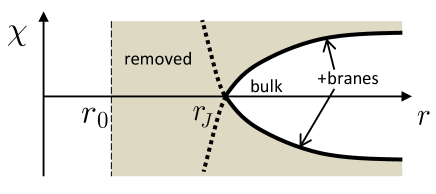
Figure 11: Global configuration composed of two $+$branes.

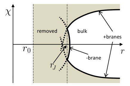
Figure 12: Global configuration composed of two $+$branes with a single $-$brane: Two +branes are connected with a $-$brane at $r=r_{J}$. In the local aspect of the junctions, this case belongs to case 1 in Sec. V.

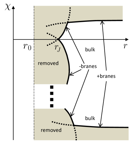
Figure 13: Global configuration composed of two $+$branes with multi $-$branes. The junction here belongs to cases 1 and 3 in Sec. V.

(a) Two $+$branes

This configuration is possible only for a positive mass bulk. From the definition it is easy to see that $h_{+}(r)$ approaches $-\pi/2$ in the limit $r\to\infty$.

For $r_{0}>r_{c}$, the possible minimum value of $r_{J}$ is $r_{*}:=\sqrt{r_{c}^{2}+r_{0}^{2}}$, and $h_{+}(r_{*})$ becomes zero. At the point $r_{J}$ satisfying $h_{+}(r_{J})=0$, we see from Eq. (35) that two branes can be connected without introducing tension $\mu_{i}$. However, the connection at $r=r_{*}$ becomes regular, and it is nothing but a single brane given in SEc. IV.1 A. For $r_{J}>r_{*}$, $h_{+}(r_{J})$ becomes negative because of its monotonically decreasing feature, and thus, we need to introduce codimension-two object with positive tensions to be consistent with Eq. (35).

Next, we consider the cases of $r_{0}<r_{c}$. We will ask if there is a case such that we can construct nontrivial configurations without introducing the codimension-two object with tension. To do so we will examine the existence of $r_{t}$ such that $h(r_{t})=0$. We first evaluate $h_{+}(r)$ at $r=r_{*}$

$$h_{+}(r_{*})=-\frac{\pi}{2}+\arctan\left(\frac{r_{0}^{2}}{\sqrt{r_{c}^{4}-r_{0}^{4}}}\right)+2\sqrt{\frac{r_{c}^{2}-r_{0}^{2}}{r_{c}^{2}+r_{0}^{2}}}.$$ (41)

We can show the positivity of this. Introducing the parameter $y$ defined by

$$r_{0}^{2}=r_{c}^{2}-y^{2},~{}(0<y<r_{c})$$ (42)

and regarding $h_{+}(r_{*})$ as the function of $y$, $F(y)$, we see

$$\frac{dF(y)}{dy}=\frac{2\left(\cos\theta_{y}\right)^{2}r_{c}^{4}}{\left(2r_{c}^{2}-y^{2}\right)^{\frac{5}{2}}}>0,$$ (43)

where

$$\theta_{y}:=\arctan\left(\frac{r_{0}^{2}-y^{2}}{\sqrt{r_{c}^{4}-r_{0}^{4}}}\right).$$ (44)

Since $F(0)=0$, the above tells us the positivity of $F(y)$, that is, $h_{+}(r_{*})>0$. Because in the asymptotic region (i.e. large $r$) $h_{+}(r)$ become negative, there is the point $r=r_{t}>r_{*}$ such that $h_{+}(r_{t})=0$. At $r=r_{t}$, therefore, we can connect two $+$branes without tension terms. If the junction point $r_{J}$ is $r_{J}>r_{t}$, we need positive tension terms to connect two $+$branes, while negative tension terms are needed if $\sqrt{2r_{0}r_{c}}<r_{J}<r_{t}$.

(b) Two $+$branes with a single $-$brane

This configuration is possible only in the case with $r_{0}<r_{c}$.

Since the $-$brane can be in the range $\sqrt{2r_{c}r_{0}}<r<r_{*}$ for the positive mass, branes should be connected in this region. We can easily obtain $h_{-}(r_{*})=0$ while we saw $h_{+}(r_{*})>0$. Since $h_{i}(r)$ is a monotonically decreasing function of $r$, $h_{+}(r)+h_{-}(r)$ is always positive for $\sqrt{2r_{c}r_{0}}<r<r_{*}$. Therefore, we see from Eq. (35) that only negative tension terms can make the branes connected.

For the negative mass bulk, the situation is similar to the positive mass case. First of all, it is easy to see $h_{-}(\bar{r}_{*})=0$ through the direct calculation, where $\bar{r}_{*}=\sqrt{r_{c}^{2}-r_{0}^{2}}$. The value of $h_{+}(\bar{r}_{*})$ is written as

$$h_{+}(\bar{r}_{*})=-\frac{\pi}{2}+\arctan\left(\frac{-r_{0}^{2}}{\sqrt{r_{c}^{4}-r_{0}^{4}}}\right)+2\sqrt{\frac{r_{c}^{2}+r_{0}^{2}}{r_{c}^{2}-r_{0}^{2}}}.$$ (45)

Introducing the parameter $y$ as

$$r_{0}^{2}=y^{2}-r_{c}^{2},\quad\mbox{with}\quad r_{c}<y<\sqrt{2}r_{c},$$ (46)

we regard $h_{+}(\bar{r}_{*})$ as the function of $y$ as

$$h_{+}(\bar{r}_{*})=F(y).$$ (47)

Here note that $F(y)$ is the same as that introduced before. Since we have already shown the positivity of $F(y)$ for $y>0$, $h_{+}(\bar{r}_{*})$ is positive. Then the monotonically decreasing property of $h_{i}(r)$ implies the positivity of $h_{+}(r)+h_{-}(r)$ for $0<r<\bar{r}_{*}$, and Eq. (35) shows us that the negative tension terms are needed to connect the branes.

As a result, for this configuration of branes, we need a negative tension term in this configuration. It is probably unphysical because of the negative energy density.

(c) Two $+$branes with multi $-$branes

This configuration is possible only for $r_{0}<r_{c}$. We can consider both cases of positive and negative mass bulks. This configuration always has the junction between two $-$branes. Let us look at the details shortly.

$h_{-}(r)$ becomes zero at $r=r_{*}$ for a positive mass bulk and at $r=\bar{r}_{*}$ for a negative mass bulk. The monotonically decreasing property of $h_{-}(r)$ leads to the positivity of $h_{-}(r)$. As a result, it is impossible to construct physically interesting solutions without introducing negative tension terms.

VII summary and discussion

In this paper we constructed the DGP braneworld with a bubble of nothing. Surprisingly, we could have the single brane solutions. This is impressive because we could not for the Randall-Sundrum braneworld. The solution with a single brane exists only for $r_{0}>r_{i}$, while for $r_{0}<r_{i}$ solutions with connected two branes can be constructed even without any matter fields on branes. Therein, the contribution of deficit structure on five-dimensional spacetime is balanced with that of a singular surface on the brane, that is, codimension-two objects in the bulk aspect. As discussed in Ref. Izumi2007 , it may be out of applicable range of the DGP-braneworld description because both contributions diverge. However, the tensionless solution sets the expectation that even in an UV completion for the DGP model less matter field is to construct the solution with two branes.

In general, the existence of the configuration founded here could lead to the semiclassical instability of DGP braneworld. If so, this may be fatal to the DGP braneworld model. But, as stressed in Ref. Witten , the supersymmetry may protect such instability. Moreover, there is a question for the initial state before the decay; that is, is the DGP vacuum with the single brane the initial state for the solution founded here? Since the size of the junction point is larger than $r_{i}$, the bubble size is also large. $r_{i}$ is expected to be a cosmological scale, and then the decay rate of the DGP vacuum to the bubble is exponentially suppressed. This is because the decay to spacetimes with large volume has a tendency to be suppressed as usual. The solutions constructed in this paper have the same asymptotic structure as the normal branch solutions on the Minkowski bulk with compactification to the extra direction. Thus, the solutions probably describe the spacetime after the decay of the normal branch. However, if one could have the solutions for the self-accelerating branch, the suppression for the decay rate to the single-brane solution might be relaxed. The detailed analysis based on quantum gravity will be interesting. There is also a problem that the self-accelerating brane is copiously nucleated Gregory2007 .

We emphasize that our solutions themselves could be worth investigating. The geometry on a single brane is like the Einstein-Rosen bridge. Since we consider the vacuum brane, any energy conditions are not violated. This is an example of wormhole spacetime which satisfies the energy conditions. The detailed analysis will be reported in the near future tomikawa .

- (1) G. R. Dvali, G. Gabadadze and M. Porrati, Phys. Lett. B 485, 208 (2000).
- (2) D. M. Capper, Nuovo Cim. A 25, 29 (1975); S. L. Adler, Phys. Rev. Lett. 44, 1567 (1980); A. Zee, Phys. Rev. Lett. 48, 295 (1982).
- (3) C. Deffayet, Phys. Lett. B 502, 199 (2001).
- (4) C. Charmousis, R. Gregory, N. Kaloper and A. Padilla, JHEP 0610, 066 (2006).
- (5) W. Fang, S. Wang, W. Hu, Z. Haiman, L. Hui and M. May, Phys. Rev. D 78, 103509 (2008).
- (6) K. Izumi and T. Tanaka, Prog. Theor. Phys. 121, 419 (2009) [arXiv:0709.0199 [gr-qc]].
- (7) K. Izumi and T. Tanaka, Prog. Theor. Phys. 121, 427 (2009) [arXiv:0810.4811 [hep-th]].
- (8) K. Koyama, Phys. Rev. D 72, 123511 (2005) [hep-th/0503191].
- (9) K. Izumi, K. Koyama and T. Tanaka, JHEP 0704, 053 (2007) [hep-th/0610282].
- (10) R. Maartens and K. Koyama, Living Rev. Rel. 13, 5 (2010) [arXiv:1004.3962 [hep-th]].
- (11) C. de Rham, G. Gabadadze and A. J. Tolley, Phys. Rev. Lett. 106, 231101 (2011).
- (12) S. F. Hassan and R. A. Rosen, JHEP 1202, 126 (2012).
- (13) C. de Rham, arXiv:1401.4173 [hep-th].
- (14) A. Padilla, Class. Quant. Grav. 21, 2899 (2004); Y. Yamashita and T. Tanaka, arXiv:1401.4336 [hep-th].
- (15) E. Witten, Nucl. Phys. B 195, 481 (1982).
- (16) L. Randall and R. Sundrum, Phys. Rev. Lett. 83, 3370 (1999); Phys. Rev. Lett. 83, 4690 (1999).
- (17) D. Ida, T. Shiromizu and H. Ochiai, Phys. Rev. D 65, 023504 (2002); H. Ochiai, D. Ida and T. Shiromizu, Prog. Theor. Phys. 107, 703 (2002).
- (18) R. Gregory, N. Kaloper, R. C. Myers and A. Padilla, JHEP 0710, 069 (2007).
- (19) K. Izumi, K. Koyama, O. Pujolas and T. Tanaka, Phys. Rev. D 76, 104041 (2007).
- (20) J. W. York, Jr., Phys. Rev. Lett. 28, 1082-1085 (1972).
- (21) G. W. Gibbons, S. W. Hawking, Phys. Rev. D15, 2752-2756 (1977).
- (22) W. Israel, Nuovo Cim. B 44S10, 1 (1966) [Erratum-ibid. B 48, 463 (1967)] [Nuovo Cim. B 44, 1 (1966)].
- (23) T. Shiromizu, K. -i. Maeda and M. Sasaki, Phys. Rev. D 62, 024012 (2000).
- (24) M. Sasaki, T. Shiromizu and K. -i. Maeda, Phys. Rev. D 62, 024008 (2000)
- (25) W. Israel, Phys. Rev. D 15, 935 (1977).
- (26) M. G. Richarte, Phys. Rev. D 82, 044021 (2010)
- (27) M. G. Richarte, Phys. Rev. D 87, 067503 (2013)
- (28) Y. Tomikawa, T. Shiromizu and K. Izumi, (to be published).