Different critical points of chiral and deconfinement phase transitions in (2+1)-dimensional fermion-gauge interacting model

Abstract

Based on the truncated Dyson-Schwinger equations for fermion and massive boson propagators in QED₃, the fermion chiral condensate and the mass singularities of the fermion propagator via the Schwinger function are investigated. It is shown that the critical point of chiral phase transition is apparently different from that of deconfinement phase transition and in Nambu phase the fermion is confined only for small gauge boson mass.

I introduction

The chiral and deconfinement phase transitions of nonperaturbative systems are important issues of continuous interests both theoretically and experimentally. Although the mechanism is unknown, the originally chiral symmetric system may undergo chiral phase transition (CPT) into a phase with dynamical chiral symmetry breaking (DCSB) which explains the origin of constituent-quark masses in QCD and underlies the success of chiral effective field theory a1 ; a2 . In the chiral limit, the order parameter of CPT is defined via the fermion propagator

$$\langle\bar{\psi}\psi\rangle=Tr[S(x\equiv 0)]=\int\frac{\mathrm{d}^{d}p}{(2\pi)^{d}}\frac{4B(p^{2})}{A^{2}(p^{2})p^{2}+B^{2}(p^{2})}.$$ (1)

The two functions $A(p^{2})$ and $B(p^{2})$ in the above equation are related to the inverse fermion propagator

$$S^{-1}(p)=i\gamma\cdot pA(p^{2})+B(p^{2}).$$ (2)

The deconfinement phase transition is then related to the observation of the free particle and also the corresponding propagator. If the full fermion propagator has no mass singularity in the timelike region, it can never be on mass shell and the free particle can never be observed where the confinement happens a3 . Accordingly, the appearance of the mass singularity in the system directly implies deconfinement. So in this way we can learn the deconfinement phase transition from the analytic structure of the fermion propagator.

To indicate DCSB and confinement, it is very suggestive to study some model that reveals the general nonperaturbative features while being simpler. Three-dimensional quantum electrodynamics (QED₃) is just such a model which has many features similar to quantum chromodynamics (QCD), such as DCSB and confinement a2 ; a3 ; a5 ; a6 ; a6a ; a6b ; a6c . Moreover, its superrenormalization obviate the ultraviolet divergence which is present in QED₄. Due to these reasons, it can serve as a toy model of QCD. In parallel with its relevance as a tool through which to develop insight into aspects of QCD, QED₃ is also found to be equivalent to the low-energy effective theories of strongly correlated electronic systems. Recently, QED₃ has been widely studied in graphene a7 ; a8 ; a9 and high-T_c cuprate superconductors a10 ; a11 ; a12 ; a13 .

The study of DCSB in QED₃ has been an active subject near 30 years since Appelquist et al. found that DCSB vanishes when the flavor of massless fermions reaches a critical number $N_{c}\approx 3.24$ a14 . They gain this conclusion by solving the truncated Dyson-Schwinger equation (DSE) for the fermion propagator in the chiral limit. Later, extensive analytical and numerical investigations showed that the existence of DCSB in QED₃ remains the same after including higher order corrections to the DSE a15 ; a16 . On the other hand, the achievement in research of the mass singularity and confinement in QED₃ is caused by a paper of P. Maris who found that the fermion is confined by the truncated DSE for the full fermion and boson propagators at $N<N_{c}$ a3 where chiral symmetry is broken. This result might imply that the existence of confinement and DCSB depend on the same boundary conditions. Moreover, the authors of Ref. a2 ; a16a pointed out that restoration of chiral symmetry and deconfinement are coincident owing to an abrupt change in the analytic properties of the fermion propagator when a nonzero scalar self-energy becomes insupportable.

Nevertheless, the above result will be altered when the gauge boson acquires a finite mass $\zeta$ through the Higgs mechanism a17 ; a18 . For a fixed $N(<N_{c})$ and with the increasing boson mass, the fermion chiral condensate falls and diminishes at a critical value $\zeta_{c}$ (which, of course, depends on $N$) and then chiral symmetry restores. Since DCSB and confinement are nonperaturbative phenomena, both of them occur in the low energy region and might disappear with the rise of boson mass. Therefore, it is very interesting to investigate whether or not both phase transitions occur at the same critical point in this case. In this paper, we will adopt the truncated DSEs for the full propagators to study the behaviors of the mass singularity and the fermion chiral condensate with a range of gauge boson mass and try to answer this question.

II Schwinger function

The Lagrangian for massless QED₃ in a general covariant gauge in Euclidean space can be written as

$$\mathcal{L}=\bar{\psi}(\not\!{\partial}-i\mathrm{e}\not\!\!{A})\psi+\frac{1}{4}F^{2}_{\sigma\nu}+\frac{1}{2\xi}(\partial_{\sigma}A_{\sigma})^{2},$$ (3)

where the 4-component spinor $\psi$ is the massless fermion field, $\xi$ is the gauge parameter. This system has chiral symmetry and the symmetry group is $U(2)$. The original $U(2)$ symmetry reduces to $U(1)\times U(1)$ when the massless fermion acquires a nonzero mass due to nonperaturbative effects. Just as mentioned in Sec. I, the chiral symmetry is broken by the dynamical generation of the fermion mass (here $N=1$). If one adopts the full boson propagator, the results of Euclidean-time Schwinger function reveal that the fermion propagator has a complex mass singularity and thus corresponds to a nonphysical observable state a3 which means the appearance of confinement. On the contrary, if the Schwinger function exhibits a real mass singularity of the propagator, the fermion is observable and the fermion is not confined a19 ; a20 . Therefore, we also adopt this method to analyze those nonperaturbative phenomena.

The Schwinger function can be written as

$$\Omega(t)=\int\mathrm{d}^{2}\vec{x}\int\frac{\mathrm{d}^{3}p}{(2\pi)^{3}}e^{i(p_{0}t+\vec{p}\cdot\vec{x})}\frac{M(p^{2})}{p^{2}+M^{2}(p^{2})}$$ (4)

with $M(p^{2})=B(p^{2})/A(p^{2})$. If there are two complex conjugate mass singularities $m^{*}=a\pm ib$ associated with the fermion propagator, the function will show an oscillating behavior

$$\Omega(t)\sim e^{-at}\cos(bt+\phi)$$ (5)

for large (Euclidean) $t$. However, the system reveals a stable observable asymptotic state with a mass $m$ for the fermion propagator, then

$$\Omega(t)\sim e^{-mt}\Rightarrow\lim_{t\rightarrow\infty}\ln\Omega(t)\sim-mt.$$ (6)

By this way, the analysis of mass singularity can be used to determine whether or not the fermion is confined. Since the Schwinger function is determined by the fermion propagator and the DSEs provide us an powerful tool to study it, we shall use the coupled gap equations to calculate this function.

III truncated DSE

Now let us turn to the calculation of $A(p^{2})$ and $B(p^{2})$. These functions can be obtained by solving DSEs for the fermion propagator,

$$S^{-1}(p)=S^{-1}_{0}(p)+\int\frac{\mathrm{d}^{3}k}{(2\pi)^{3}}[\gamma_{\sigma}S(k)\Gamma_{\nu}(p,k)D_{\sigma\nu}(q)],$$ (7)

where $\Gamma_{\nu}(p,k)$ is the full fermion-photon vertex and $q=p-k$. The coupling constant $\alpha=\mathrm{e}^{2}$ has dimension one and provides us with a mass scale. For simplicity, in this paper temperature, mass and momentum are all measured in unit of $\alpha$, namely, we choose a kind of natural units in which $\alpha=1$. Form Eq. (2) and Eq. (7), we obtain the equation satisfied by $A(p^{2})$ and $B(p^{2})$

$$A(p^{2}) = 1-\frac{1}{4p^{2}}\int\frac{\mathrm{d}^{3}k}{(2\pi)^{3}}Tr[i(\gamma p)\gamma_{\sigma}S(k)\Gamma_{\nu}(p,k)D_{\sigma\nu}(q)],$$ (8)

$$B(p^{2}) = \frac{1}{4}\int\frac{\mathrm{d}^{3}k}{(2\pi)^{3}}Tr\left[\gamma_{\sigma}S(k)\Gamma_{\nu}(p,k)D_{\sigma\nu}(q)\right].$$ (9)

Another involved function $D_{\sigma\nu}(q)$ is the full gauge boson propagator which is given bya17 ; a18

$$D_{\sigma\nu}(q)=\frac{\delta_{\sigma\nu}-q_{\sigma}q_{\nu}/q^{2}}{q^{2}[1+\Pi(q^{2})]+\zeta^{2}}+\xi\frac{q_{\sigma}q_{\nu}}{q^{4}},$$ (10)

where $\Pi(q^{2})$ is the vacuum polarization for the gauge boson which is satisfied by the polarization tensor

$$\Pi_{\sigma\nu}(q^{2})=-\int\frac{\mathrm{d}^{3}k}{(2\pi)^{3}}Tr\left[S(k)\gamma_{\sigma}S(q+k)\Gamma_{\nu}(p,k)\right]$$ (11)

and $\zeta$ is the gauge boson mass which is acquired though Higgs mechanism which happens when the gauge field interacts with a scalar filed in the phase with spontaneous gauge symmetry breaking (Here, we adopt the massive boson propagator to investigate the oscillation behavior of Schwinger function in DCSB phase, more details about Higgs mechanism in QED₃ can be found in Ref. a17 ; a18a ).

Using the relation between the vacuum polarization $\Pi(q^{2})$ and $\Pi_{\sigma\nu}(q^{2})$,

$$\Pi_{\sigma\nu}(q^{2})=(q^{2}\delta_{\sigma\nu}-q_{\sigma}q_{\nu})\Pi(q^{2}),$$ (12)

we can obtain an equation for $\Pi(q^{2})$ which has an ultraviolet divergence. Fortunately, it is present only in the longitudinal part and is proportional to $\delta_{\sigma\nu}$. This divergence can be removed by the projection operator

$$\mathcal{P}_{\sigma\nu}=\delta_{\sigma\nu}-3\frac{q_{\sigma}q_{\nu}}{q^{2}},$$ (13)

and then we obtain a finite vacuum polarizationa5a ; a6 .

Finally, we choose to work in the Landau gauge, since the Landau gauge is the most convenient and commonly used one. Once the fermion-boson vertex is known, we immediately obtain the truncated DSEs for the fermion propagator and then analyze the deconfinement and chiral phase transitions in this Higgs model.

III.1 Rainbow approximation

The simplest and most commonly used truncated scheme for the DSEs is the rainbow approximation,

$$\Gamma_{\nu}\rightarrow\gamma_{\nu},$$ (14)

since it gives us rainbow diagrams in the fermion DSE and ladder diagrams in the Bethe-salpeter equation for the fermion-antifermion bound state amplitude. In the framework of this approximation, the coupled equations for massless fermion and massive boson propagators reduce to the three coupled equations for $A(p^{2})$, $B(p^{2})$ and $\Pi(q^{2})$,

$$A(p^{2}) = 1+\int\frac{\mathrm{d}^{3}k}{(2\pi)^{3}}\frac{2A(k^{2})(pq)(kq)/q^{2}}{p^{2}G(k^{2})[q^{2}(1+\Pi(q^{2}))+\zeta^{2}]},$$ (15)

$$B(p^{2}) = \int\frac{\mathrm{d}^{3}k}{(2\pi)^{3}}\frac{2B(k^{2})}{G(k^{2})[q^{2}(1+\Pi(q^{2}))+\zeta^{2}]},$$ (16)

$$\Pi(q^{2}) = \int\frac{\mathrm{d}^{3}k}{(2\pi)^{3}}\frac{2A(k^{2})A(p^{2})}{q^{2}G(k^{2})G(p^{2})}\times$$ (17)

$$[2k^{2}-4(k\cdot q)-6(k\cdot q)^{2}/q^{2}],$$

with $G(k^{2})=A^{2}(k^{2})k^{2}+B^{2}(k^{2})$. By application of iterative methods, we can obtain $A,~{}B$ and $\Pi$.

III.2 Improved scheme for DSE

To improve the truncated scheme for DSE, there are several attempts to determine the functional form for the full fermion-gauge-boson vertex a20a ; a21 ; a22 ; a23 , but none of them completely resolve the problem. However, the Ward-Takahashi identity

$$(p-k)_{\nu}\Gamma_{\nu}(p,k)=S^{-1}(p)-S^{-1}(k),$$ (18)

provides us an effectual tool to obtain a reasonable ansatze for the full vertex a24 . The portion of the dressed vertex which is free of kinematic singularities, i.e. BC vertex, can be written as,

$$\Gamma_{\nu}(p,k) = \frac{A(p^{2})+A(k^{2})}{2}\gamma_{\nu}+\frac{B(p^{2})-B(k^{2})}{p^{2}-k^{2}}(p+k)_{\nu}$$ (19)

$$+(\not\!p+\not\!k)\frac{A(p^{2})-A(k^{2})}{2(p^{2}-k^{2})}(p+k)_{\nu}.$$

Since the numerical results obtained using the first part of the vertex coincide very well with earlier investigations a16 , we choose this one as a suitable ansatze

$$\Gamma_{\nu}^{BC_{1}}(p,k)\simeq\frac{1}{2}\left[A(p^{2})+A(k^{2})\right]\gamma_{\nu}$$ (20)

to be used in our calculation. Following the procedure in rainbow approximation, we also obtain the three coupled equations for $A(p^{2}),~{}B(p^{2})$ and $\Pi(q^{2})$ in the improved truncated scheme for DSEs,

$$A(p^{2})=1+\int\frac{\mathrm{d}^{3}k}{(2\pi)^{3}}\frac{A(k^{2})[A(p^{2})+A(k^{2})](pq)(kq)/q^{2}}{p^{2}G(k^{2})[q^{2}(1+\Pi(q^{2}))+\zeta^{2}]},$$ (21)

$$B(p^{2})=\int\frac{\mathrm{d}^{3}k}{(2\pi)^{3}}\frac{[A(p^{2})+A(k^{2})]B(k^{2})}{G(k^{2})[q^{2}(1+\Pi(q^{2}))+\zeta^{2}]},$$ (22)

$$\Pi(q^{2})=\int\frac{\mathrm{d}^{3}k}{(2\pi)^{3}}\frac{A(k^{2})A(p^{2})[A(p^{2})+A(k^{2})]}{q^{2}G(k^{2})G(p^{2})}\times$$

$$~{}~{}~{}~{}~{}~{}~{}~{}~{}~{}~{}~{}~{}~{}~{}~{}~{}~{}~{}~{}[2k^{2}-4(k\cdot q)-6(k\cdot q)^{2}/q^{2}],$$ (23)

IV numerical results

After solving the above coupled DSEs in rainbow approximation by means of the iteration method, we can obtain the three function $A,~{}B,~{}\Pi$ for the propagator and plot them in Fig. 1.

Figure 1: The typical behaviors of $A(p^{2}),~{}B(p^{2}),~{}\Pi(q^{2})$ (Left) and their infrared values (Right) as functions of the boson mass in DCSB phase.

From Fig. 1 it can be seen that $A(p^{2})$ increases with increasing momenta but almost equal to one at large $p^{2}$. In the range of small momenta, it decreases but does not vanish when $p^{2}\rightarrow 0$. Both of the other two functions $B(p^{2})$ and $\Pi(q^{2})$ decrease at large momenta but their rates of decreasing are different. $B(p^{2})$ decreases as rapidly as $\sim 1/p^{2}$, while $\Pi(q^{2})$ decreases as rapidly as $\sim 1/\sqrt{q^{2}}$. In addition, all the three functions are constant in the infrared region. Thus, we can obtain the values of the corresponding functions $A,~{}B$ and $\Pi$ at zero momenta, which, as functions of the gauge boson mass $\zeta$, are also shown in Fig. 1. As $\zeta$ increases, both $A(0)$ and $B(0)$ decrease, and $B(0)$ vanishes when $\zeta$ reaches a critical gauge boson mass $\zeta^{R}_{c}\approx 0.102$, whereas the function $\Pi(0)$ rises and diverges at the same critical boson mass $\zeta^{R}_{c}$. Based on Eq. (1), the critical boson mass can be regarded as the point of chiral phase transition.

Then, substituting the obtained $A$ and $B$ into Eq. (4), we immediately obtain the behavior of the Schwinger function with nonzero boson mass which is shown in Fig. 2. At small $\zeta$, the Schwinger function reveals its typical oscillating behavior which illustrates the conjugate mass singularities like $m^{*}=a\pm ib$

$$m^{*} \sim 0.043\pm 0.063i~{}\mathrm{at}~{}\zeta=0.01,$$ (24)

$$m^{*} \sim 0.023\pm 0.025i~{}\mathrm{at}~{}\zeta=0.06,$$ (25)

associated with the fermion propagator and thus the free particle can never be observed where the fermion is confined. As the rise of $\zeta$, the oscillating behavior remains but it vanishes at another critical value $\zeta^{R}_{dc}\approx 0.068$ and around which both of the propagators do not exhibit any singularity.

Beyond $\zeta^{R}_{dc}$, the function $\ln[\Omega(t)]\sim-mt$ where the stable asymptotic state of the fermion is observable

$$m \approx 0.021~{}\mathrm{at}~{}\zeta=0.07,$$ (26)

$$m \approx 0.0041~{}\mathrm{at}~{}\zeta=0.09$$ (27)

and hence the deconfinement phase transition happens, but the DCSB remains. With the enlargement of $\zeta$, the absolute slope of $\ln[\Omega(t)]$ decreases and $m$ disappears at $\zeta^{R}_{c}$.

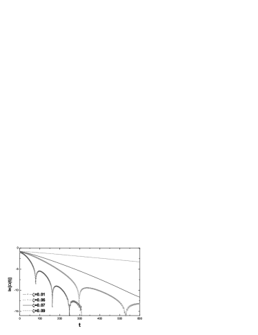
Figure 2: Logarithm of the absolute value of the Schwinger function with several $\zeta$ for the rainbow approximation.

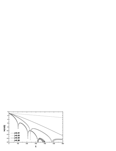
Figure 3: The value of fermion chiral condensate (top) and the logarithm (bottom) in the framework of BC₁ vertex with a range of $\zeta$.

To validate the difference between $\zeta_{c}$ and $\zeta_{dc}$, we also give the behavior of the Schwinger function beyond rainbow approximation in Fig. 3. In the BC₁ truncated scheme for DSE, the oscillation of the Schwinger function only appears at small $\zeta$, which denotes the existence of confinement, but it disappears at $\zeta^{BC_{1}}_{dc}\approx 0.038$, which exhibits that deconfinement phase transition occurs but here $\langle\bar{\psi}\psi\rangle\neq 0$. As the rise of $\zeta$, the Schwinger function shows the real mass singularity of the propagator and chiral symmetry gets restored when the boson mass reaches $\zeta^{BC_{1}}_{c}\approx 0.071$.

V conclusions

The primary goal of this paper is to investigate chiral and deconfinement phase transition by application of an Abelian Higgs model through a continuum study of the Schwinger function. Based on the rainbow approximation of the truncated DSEs for the fermion propagator and numerical model calculations, we study the behavior of the Schwinger function and the fermion chiral condensate. It is found that, with the rise of the gauge boson mass, the vanishing point ($\zeta_{dc}$) of the oscillation behavior of the Schwinger function is apparently less than that of the fermion chiral condensate and each of the propagators does not reveal any singularity near $\zeta_{dc}$. To make know the difference between the two critical points, we also work in an improved scheme for the truncated DSEs and show that the above conclusion remains despite the two critical numerical values alter. The result indicates that, with the increasing gauge boson mass in the chiral model, the occurrence of de-confinement phase transition is apparently earlier than that of chiral phase transition.

VI acknowledgements

We would like to thank Prof. Wei-min Sun and Guo-zhu Liu for their helpful discussions. This work was supported by the National Natural Science Foundation of China (under Grant Nos. 11105029, 11275097 and 11205227) and the Fundamental Research Funds for the Central Universities (under Grant No 2242014R30011).

References

- (1) C.D. Roberts, Prog. Part. Nucl. Phys. 61, 50 (2008).
- (2) A. Bashir, A. Raya, I.C. Cloet and C.D. Roberts, Phys. Rev. C 78, 055201 (2008).
- (3) P. Maris, Phys. Rev. D 52, 6087 (1995).
- (4) M. R. Pennington and D. Walsh, Phys. Lett. B 253, 246 (1991).
- (5) C.J. Burden, J. Praschifka, and C.D. Roberts, Phys. Rev. D 46, 2695 (1992).
- (6) H.T. Feng, B. Wang, W.M. Sun, and H.S. Zong, Euro. Phys. J. C 73, 2444 (2013).
- (7) H.T. Feng, B. Wang, W.M. Sun, and H.S. Zong, Phys. Rev. D 86, 105042 (2012).
- (8) H.T. Feng, Y.Q. Zhou, P.L. Yin, and H.S. Zong, Phys. Rev. D 88, 125022 (2013).
- (9) D.V. Khveshchenko, Phys. Rev. Lett. 87, 246802 (2001).
- (10) V.P. Gusynin and S.G. Sharapov, Phys. Rev. Lett. 95, 146801 (2005).
- (11) J.E. Drut and T.A. Lahde, Phys. Rev. Lett. 102, 026802 (2009).
- (12) N. Dorey and N. E. Mavromatos, Nucl. Phys. B386, 614 (1992).
- (13) M. Franz, Z. Tesanovic, and O. Vafek, Phys. Rev. B 66, 054535 (2002).
- (14) W. Rantner and X.G. Wen, Phys. Rev. B 66, 144501 (2002).
- (15) P.A. Lee, N. Nagaosa, and X.G. Wen, Rev. Mod. Phys. 78, 17 (2006).
- (16) T. Appelquist, D. Nash, and L.C.R. Wijewardhana, Phys. Rev. Lett. 60, 2575 (1988).
- (17) D. Nash, Phys. Rev. Lett. 62, 3024 (1989).
- (18) C.S. Fischer, R. Alkofer, T. Dahm, and P. Maris, Phys. Rev. D 70, 073007 (2004).
- (19) C.P. Hofmann, A. Raya, and S.S. Madrigal, Phys. Rev. D 82, 096011 ( 2010).
- (20) G.Z. Liu and G. Cheng, Phys. Rev. D 67, 065010(2003).
- (21) H.T. Feng, W.M. Sun, F. Hu, and H.S. Zong, Inter. J. Mod. Phys. A 20(13), 2753 (2005).
- (22) J.F. Li, H.T. Feng, Y. Jiang, W.M. Sun, and H.S. Zong, Mod. Phys. Lett. A 27, 1250026 (2012).
- (23) N. Brown and M.R. Pennington, Phys. Rev. D 39, 2723 (1989).
- (24) L.C.L. Hollenberg, C.D. Roberts, and B.H.J. McKellar, Phys. Rev. C 46, 2057 (1992).
- (25) C.D. Roberts and A.G. Williams, Prog. Part. Nucl. Phys. 33, 477(1994).
- (26) D.C. Curtis and M.R. Pennington, Phys. Rev. D 42, 4165 (1990).
- (27) M.R. Pennington and D. Walsh, Phys. Lett. B 253, 246 (1991).
- (28) K.-I. Kondo and P. Maris, Phys. Rev. Lett. 74, 18 (1995).
- (29) G.W. Semenoff, P. Suranyi, and L.C.R. Wijewardhana, Phys. Rev. D 50, 1060 (1994).
- (30) J.S. Ball and T.W. Chiu, Phys. Rev. D 22, 2542 (1980).