MCMC algorithms for Bayesian variable selection in the logistic regression model for large-scale genomic applications

Abstract.

In large-scale genomic applications vast numbers of molecular features are scanned in order to find a small number of candidates which are linked to a particular disease or phenotype. This is a variable selection problem in the “large $p$, small $n$” paradigm where many more variables than samples are available. Additionally, a complex dependence structure is often observed among the markers/genes due to their joint involvement in biological processes and pathways.

Bayesian variable selection methods that introduce sparseness through additional priors on the model size are well suited to the problem. However, the model space is very large and standard Markov chain Monte Carlo (MCMC) algorithms such as a Gibbs sampler sweeping over all $p$ variables in each iteration are often computationally infeasible. We propose to employ the dependence structure in the data to decide which variables should always be updated together and which are nearly conditionally independent and hence do not need to be considered together.

Here, we focus on binary classification applications. We follow the implementation of the Bayesian probit regression model by Albert and Chib (1993) and the Bayesian logistic regression model by Holmes and Held (2006) which both lead to marginal Gaussian distributions. We investigate several MCMC samplers using the dependence structure in different ways. The mixing and convergence performances of the resulting Markov chains are evaluated and compared to standard samplers in two simulation studies and in an application to a real gene expression data set.

1. Introduction

Advances in high-throughput technologies in the medical and biosciences since the mid-1990s have resulted in a shift towards datasets with a vast number of variables $p$ and a comparably small sample size $n$. In this setup we typically have many more variables than samples, i.e. $p>>n$. It is often reasonable to assume that only a very small subset of all measured variables is sufficient to predict the biological condition or phenotype of interest. This leads to the introduction of sparse regression models where the estimated regression coefficients $\beta_{i}$ ($i=1,...,p$) are assumed to be zero for most input variables. In a Bayesian framework this can be achieved easily by introducing a binary indicator vector $\boldsymbol{\gamma}=(\gamma_{1},...,\gamma_{p})$, which indicates whether a variable $\boldsymbol{x}_{i}$ is considered to be included in the model ($\gamma_{i}=1$) or not ($\gamma_{i}=0$). Sparsity is induced by setting the prior probability of including a variable to a small value, reflecting the expected model size.

Here, we are particularly interested in applying this Bayesian variable selection (BVS) framework in the binary regression context for modelling the effect of a high-dimensional gene expression data matrix $\boldsymbol{x}\in\mathbb{R}^{n\times p}$ (with $p>>n$) on a dichotomous outcome vector $\boldsymbol{y}\in\{0,1\}^{n}$ such as treatment response (response versus non-response) or the categorisation of samples into tumour samples versus healthy tissue. Throughout this manuscript we sometimes refer to covariates $\boldsymbol{x}_{i}$ ($i=1,...,p$) as genes or probe sets. Other authors who have used BVS in this context have focussed on the probit regression model for which an auxiliary variable implementation is available that leads to conjugate Gaussian priors (Albert and Chib 1993). In recent years there have been many attempts to develop similar data augmentation methods for the logistic regression model, for example Holmes and Held (2006), Frühwirth-Schnatter and Frühwirth (2010), Gramacy and Polson (2012), Polson et al. (2013) (see Polson et al. (2013) for a recent overview). In this manuscript we apply the approach by Holmes and Held (2006), which leads to marginal Gaussian distributions after the introduction of an additional layer of parameters in the Bayesian hierarchical model.

Because of the vastness of the model space, posterior inference by Markov chain Monte Carlo (MCMC) using standard samplers such as full Gibbs sampling is computationally very demanding, which is a big hurdle for practical applications. A Bayesian variable selection model with Gibbs sampling has therefore not been used often in an application setting with several thousand variables, one example being an application based on microarray gene expression data for binary classification by probit regression by Lee et al. (2003). With a view to these practical limitations of the Gibbs sampler Hans et al. (2007) proposed the shotgun stochastic search (SSS) algorithm as an alternative method. SSS is related to MCMC but does not sample from the full posterior distribution. Instead it performs a stochastic search in the model space to quickly hone into the regions of high posterior probability.

Other approaches have remained in the MCMC setting and attempted to replace the Gibbs sampler by faster MCMC algorithms. In particular, an add/delete(/swap) Metropolis-Hastings algorithm has been proposed, where in each iteration the state of one variable is proposed to be swapped from $\gamma_{i}=0$ to $\gamma_{i}=1$ (add move) or from $\gamma_{i}=1$ to $\gamma_{i}=0$ (delete move) (Brown et al. 1998b, Sha et al. 2004). Sometimes a swap move is included as well where the states of two variables $\gamma_{i}$ and $\gamma_{k}$ are proposed to be exchanged. The add/delete(/swap) algorithm is computationally very fast. However, it has been noted that such proposals experience problems if $p>>n$ in that the acceptance probability for deleting variables tends to zero (Hans et al. 2007). Also, mixing is a problem, since only one or two randomly selected variables are proposed to be updated in each iteration. This is especially problematic with $p>>n$, where one usually assumes sparseness, i.e. only a small number of covariates are related to the response variable, while most do not carry information regarding the response. In this situation, the randomly selected covariates are very unlikely to be related to the response and will thus not be updated in most MCMC iterations. In addition, the sampler does not make use of the correlation structure among the covariates, which increases the likelihood of the sampler getting stuck: Imagine a situation where two covariates $\boldsymbol{x}_{i}$ and $\boldsymbol{x}_{k}$ are moderately correlated with each other, and $\boldsymbol{x}_{i}$ has a strong effect on the response while $\boldsymbol{x}_{k}$ only has a comparably small effect on $\boldsymbol{y}$. If $\boldsymbol{x}_{k}$ is included first by the Metropolis-Hastings sampler then it might prevent the inclusion $\boldsymbol{x}_{i}$ as long as it remains in the model, although inclusion of $\boldsymbol{x}_{i}$ might result in a better model fit.

A complex dependence structure is often observed among genes in high-throughput biological data due to their joint involvement in biological processes and pathways. Luckily it is often reasonable to assume that the conditional dependence structure for such data is sparse, that is each of the variables is only correlated with a small number of covariates when conditioning on all other variables in the data set (e.g. West 2003). Thus it might not be necessary to do full Gibbs sampling updating all covariates in each iteration in order to avoid mixing problems as the one described above. Rather, one could enjoy the same fast mixing by exploiting the dependence structure in the data to decide which variables should always be updated together and which are nearly conditionally independent and hence do not need to be considered together. Such a sampler is not as computationally demanding as full Gibbs sampling and should result in better mixing relative to the required computation time per iteration.

All these MCMC samplers can be implemented within a parallel tempering framework (Geyer 1991). Parallel tempering methods are designed to help overcome local optima by running different Markov chains at higher temperatures in parallel with the original Markov chain and proposing to switch the states of the chains in an additional Metropolis-Hastings step. The aim is to trickle the faster mixing effects in the higher-temperature chains down to the original sampler, while still maintaining the proper target invariant distribution for the original chain.

In the following section the Bayesian variable selection model for logistic regression is presented. Then, the MCMC algorithm for sampling from the logistic variable selection model is described including the add/delete and Gibbs samplers. We develop our alternative samplers (which we call neighbourhood samplers) using the dependence structure between covariates and we outline how we estimate the dependence structure. The mixing and convergence performances of the MCMC samplers are evaluated and compared in two simulation studies in Section 6. The add/delete sampler and one representative neighbourhood Gibbs sampler are applied to a real gene expression data set in Section 7, where we combine these samplers with parallel tempering. The paper concludes with a discussion of our findings.

The software for sampling from the logistic as well as the probit BVS model is available as MATLAB (The MathWorks 2006) toolbox BVS (http://www.bgx.org.uk/software.html). Most options of the logistic BVS model are also implemented in the R statistical computing environment (R Core Team 2013) with computationally intensive parts of the MCMC algorithm outsourced to C, in the bvsflex package available on R-forge
(http://bvsflex.r-forge.r-project.org) (Zucknick 2013).

2. Bayesian variable selection for logistic regression

A conjugate formulation for a Bayesian binary regression model with response $\boldsymbol{y}\in\{0,1\}^{n}$ was first developed for the probit model by Albert and Chib (1993) by introducing a latent variable $z_{j}$ for all $j=1,...,n$, which has a normal prior distribution and hence a conjugate normal posterior distribution. The binary response $y_{j}$ for subject $j=1,...,n$ is modelled by the probit link in a deterministic manner:

(3) $$y_{j} = \left\{\begin{array}[]{ll}1&\mbox{if }z_{j}>0\\ 0&\mbox{otherwise}\end{array}\right.$$

$$z_{j} = \boldsymbol{x}_{j}\boldsymbol{\beta}+\epsilon_{j}$$

$$\epsilon_{j} \sim N(0,1)$$

$$\boldsymbol{\beta} \sim N(\boldsymbol{b},\boldsymbol{v}),$$

where the regression coefficient vector $\boldsymbol{\beta}=(\beta_{i})_{i=1}^{p}$ has a normal prior distribution with mean vector $\boldsymbol{b}$ and covariance matrix $\boldsymbol{v}$.

Often, the logistic regression model is preferred over the probit model in statistical applications, as it provides regression coefficients that are more interpretable due to their connection to odds ratios. Holmes and Held (2006) have developed an auxiliary variable formulation of the logistic model in the Bayesian context, which uses a latent variable $\boldsymbol{z}$ with conjugate normal priors:

(6) $$y_{j} = \left\{\begin{array}[]{ll}1&\mbox{if }z_{j}>0\\ 0&\mbox{otherwise}\end{array}\right.$$

$$z_{j} = \boldsymbol{x}_{j}\boldsymbol{\beta}+\epsilon_{j}$$

$$\epsilon_{j} \sim N(0,\lambda_{jj})$$

$$\lambda_{jj} = (2\phi_{j})^{2}$$

$$\phi_{j} \sim$$ Kolmogorov-Smirnov (i.i.d.)

$$\boldsymbol{\beta} \sim N(\boldsymbol{b},\boldsymbol{v}).$$

The auxiliary variables $\phi_{j}$, $j=1,...,n$, are independent random variables following the Kolmogorov-Smirnov distribution. This leads to a normal scale mixture distribution for $\epsilon_{j}$ resulting in a marginal logistic distribution, so that this model is equivalent to a Bayesian logistic regression model (Andrews and Mallows 1974). Since the prior distribution of $\boldsymbol{\beta}$ is normal, the posterior distribution of $\boldsymbol{\beta}$ is still normal with mean $\boldsymbol{B}$ and covariance matrix $\boldsymbol{V}$, according to standard Bayesian modelling theory (e.g. Lindley and Smith 1972):

(7) $$\boldsymbol{\beta}|\boldsymbol{z},\boldsymbol{\lambda} \sim N(\boldsymbol{B},\boldsymbol{V})$$

$$\boldsymbol{B} = \boldsymbol{V}(\boldsymbol{v}^{-1}\boldsymbol{b}+\boldsymbol{x}^{\prime}\boldsymbol{\lambda}^{-1}\boldsymbol{z})$$

$$\boldsymbol{V} = (\boldsymbol{v}^{-1}+\boldsymbol{x}^{\prime}\boldsymbol{\lambda}^{-1}\boldsymbol{x})^{-1}$$

$$\boldsymbol{\lambda}^{-1} = \mbox{diag}(\lambda_{11},...,\lambda_{nn})^{-1}.$$

Holmes and Held (2006) extend their Bayesian logistic regression model to incorporate variable selection by including a covariate indicator variable $\boldsymbol{\gamma}\in\{0,1\}^{p}$. We denote the size of the active covariate set by $p_{\gamma}=\sum_{i=1}^{p}{I(\gamma_{i}=1)}$, where $I$ is an indicator function. Then, the Bayesian logistic model for variable selection is given by

(10) $$y_{j} = \left\{\begin{array}[]{ll}1&\mbox{if }z_{\gamma j}>0\\ 0&\mbox{otherwise}\end{array}\right.$$

$$z_{\gamma j} = \boldsymbol{x}_{\gamma j}\boldsymbol{\beta}_{\gamma}+\epsilon_{j}$$

$$\epsilon_{j} \sim N(0,\lambda_{jj})$$

$$\lambda_{jj} = (2\phi_{j})^{2}$$

$$\phi_{j} \sim$$ Kolmogorov-Smirnov (i.i.d.)

$$\boldsymbol{\beta}_{\gamma} \sim p(\boldsymbol{\beta}_{\gamma})$$

$$\boldsymbol{\gamma} \sim p(\boldsymbol{\gamma})=\prod_{i=1}^{p}{\pi_{i}^{\gamma_{i}}(1-\pi_{i})^{1-\gamma_{i}}}$$

The $\boldsymbol{\gamma}$ subscripts indicate that the model is only defined for those components $i$ for which $\gamma_{i}=1$. The prior on the model space is specified in terms of the prior distribution $p(\boldsymbol{\gamma})$, which in this case is a binomial prior with individual prior probabilities $\pi_{i}$ for each indicator variable $\gamma_{i}$. Throughout this paper we assume constant prior probabilities $\pi_{i}=p^{*}/p$ for all $\gamma_{i}$ so that the expected number of covariates a priori is $p^{*}$. The prior distribution on the regression coefficient vector $\boldsymbol{\beta}_{\gamma}$ is $N(\boldsymbol{b}_{\gamma},\boldsymbol{v}_{\gamma})$, where $\boldsymbol{b}_{\gamma}=\boldsymbol{0}_{p_{\gamma}}$ is typically chosen ($\boldsymbol{0}_{p_{\gamma}}$ denotes the zero vector of length $p_{\gamma}$). Throughout this manuscript we use the independence prior, which is defined by $\boldsymbol{v}_{\gamma}=c^{2}\boldsymbol{I}_{p_{\gamma}}$, where $\boldsymbol{I}_{p_{\gamma}}$ is the identity matrix of dimension $p_{\gamma}\times p_{\gamma}$. An alternative would be Zellner’s g-prior, i.e. if $\boldsymbol{v}_{\gamma}=c^{2}(\boldsymbol{x}_{\gamma}^{\prime}\boldsymbol{x}_{\gamma})^{-1}$ is chosen, where $\boldsymbol{x}_{\gamma}$ is a sub-matrix of $\boldsymbol{x}$ where only those columns $i\in\{1,...,p\}$ are kept for which $\gamma_{i}=1$.

The hierarchical logistic regression model (10) leads to the following joint posterior distribution for $\{\boldsymbol{\beta}_{\gamma},\boldsymbol{\gamma},\boldsymbol{z},\boldsymbol{\lambda}\}$ (Holmes and Held 2006):

$$p(\boldsymbol{\beta}_{\gamma},\boldsymbol{\gamma},\boldsymbol{z},\boldsymbol{\lambda}|\boldsymbol{x},\boldsymbol{y}) \propto p(\boldsymbol{\beta}_{\gamma},\boldsymbol{\gamma},\boldsymbol{z},\boldsymbol{\lambda},\boldsymbol{y}|\boldsymbol{x})$$

$$= p(\boldsymbol{y}|\boldsymbol{z})p(\boldsymbol{z}|\boldsymbol{\lambda},\boldsymbol{\beta},\boldsymbol{\gamma},\boldsymbol{x})p(\boldsymbol{\beta}_{\gamma}|\boldsymbol{\gamma})p(\boldsymbol{\gamma})p(\boldsymbol{\lambda})$$

where

$$p(\lambda_{jj})\sim\frac{1}{4\sqrt{\lambda_{jj}}}KS(0.5\sqrt{\lambda_{jj}})$$

and

$$p(\boldsymbol{z}|\boldsymbol{\lambda},\boldsymbol{\beta},\boldsymbol{\gamma},\boldsymbol{x})=N(\boldsymbol{x}_{\gamma}\boldsymbol{\beta}_{\gamma},\boldsymbol{\lambda}).$$

3. MCMC algorithms

Variables are quite highly correlated due to the way they are constructed, especially $\boldsymbol{\beta}_{\gamma}$ with $\boldsymbol{\gamma}$ and $\boldsymbol{z}$ with $\boldsymbol{\lambda}$. We can implement the MCMC sampler efficiently by using a blocked Gibbs sampler where $\{\boldsymbol{z},\boldsymbol{\lambda}\}$ and $\{\boldsymbol{\gamma},\boldsymbol{\beta}_{\gamma}\}$ are updated jointly, respectively. Such a sampler has the additional advantage that it allows for efficient updating within the neighbourhoods, because sampling from all distributions involved can be done in a fast manner, see Table 1 below.

Table 1. Outline of MCMC sampling algorithm: Gibbs sampling from full conditional distributions $p(\boldsymbol{z},\boldsymbol{\lambda}|\boldsymbol{\beta},\boldsymbol{\gamma},\boldsymbol{x},\boldsymbol{y})$ and $p(\boldsymbol{\beta}_{\gamma},\boldsymbol{\gamma}|\boldsymbol{z},\boldsymbol{\lambda},\boldsymbol{x})$. Note that by $\mbox{Logistic}(\mu,\sigma)$ we denote a logistic distribution with location parameter $\mu$ and scale parameter $\sigma>0$.

(1)	Sample from $p(\boldsymbol{z},\boldsymbol{\lambda}|\boldsymbol{\beta},\boldsymbol{\gamma},\boldsymbol{x},\boldsymbol{y})=p(\boldsymbol{\lambda}|\boldsymbol{z},\boldsymbol{\beta},\boldsymbol{\gamma},\boldsymbol{x})p(\boldsymbol{z}|\boldsymbol{\beta},\boldsymbol{\gamma},\boldsymbol{x},\boldsymbol{y})$
(a)	$p(\lambda_{jj}|z_{j},\boldsymbol{\beta},\boldsymbol{\gamma},\boldsymbol{x}_{j})\propto p(z_{j}|\lambda_{jj},\boldsymbol{\beta},\boldsymbol{\gamma},\boldsymbol{x}_{j})p(\lambda_{jj})$ $\forall j$, where	Rejection sampling
	$p(z_{j}|\lambda_{jj},\boldsymbol{\beta},\boldsymbol{\gamma},\boldsymbol{x}_{j})=N(\boldsymbol{x}_{\gamma,j}^{\prime}\boldsymbol{\beta}_{\gamma},\lambda_{jj})$ and $p(\lambda_{jj})=\frac{1}{4\sqrt{\lambda_{jj}}}\mbox{KS}(0.5\sqrt{\lambda_{jj}})$
(b)	$p(z_{j}|\boldsymbol{\beta},\boldsymbol{\gamma},\boldsymbol{x},\boldsymbol{y})=\left\{\begin{array}[]{ll}\mbox{Logistic}(\boldsymbol{x}_{\gamma,j}^{\prime}\boldsymbol{\beta}_{\gamma},1)I(z_{j}>0),&y_{j}=1\\ \mbox{Logistic}(\boldsymbol{x}_{\gamma,j}^{\prime}\boldsymbol{\beta}_{\gamma},1)I(z_{j}\leq 0),&y_{j}=0\end{array}\right.$ $\forall j$	Inversion method
(2)	Sample from $p(\boldsymbol{\beta}_{\gamma},\boldsymbol{\gamma}|\boldsymbol{z},\boldsymbol{\lambda},\boldsymbol{x})=p(\boldsymbol{\gamma}|\boldsymbol{z},\boldsymbol{\lambda},\boldsymbol{x})p(\boldsymbol{\beta}_{\gamma}|\boldsymbol{\gamma},\boldsymbol{z},\boldsymbol{\lambda},\boldsymbol{x})$
(a)	$p(\boldsymbol{\gamma}|\boldsymbol{z},\boldsymbol{\lambda},\boldsymbol{x})\propto p(\boldsymbol{z}|\boldsymbol{\lambda},\boldsymbol{x},\boldsymbol{\gamma})p(\boldsymbol{\gamma})$	Various samplers
		(see Section 5)
(b)	$p(\boldsymbol{\beta}_{\gamma}|\boldsymbol{\gamma},\boldsymbol{z},\boldsymbol{\lambda},\boldsymbol{x})=N(\boldsymbol{B}_{\gamma},\boldsymbol{V}_{\gamma})$, where	Direct sampling
	$\boldsymbol{B}_{\gamma}=\boldsymbol{V}_{\gamma}\boldsymbol{x}_{\gamma}^{\prime}\boldsymbol{\lambda}^{-1}\boldsymbol{z}$ and $\boldsymbol{V}_{\gamma}=(\boldsymbol{x}_{\gamma}^{\prime}\boldsymbol{\lambda}^{-1}\boldsymbol{x}_{\gamma}+\boldsymbol{v}_{\gamma}^{-1})^{-1}$

Holmes and Held (2006) propose to use an add/delete proposal distribution $q(\boldsymbol{\gamma})$ in the Metropolis-Hastings step for updating $p(\boldsymbol{\beta}_{\gamma},\boldsymbol{\gamma}|\boldsymbol{z},\lambda,\boldsymbol{x})$, which is similar to the add/delete/swap algorithm proposed by for example Brown et al. (1998b). That is, the proposal distribution for a randomly selected $\gamma_{i}$ is defined as

(12) $$q(\gamma^{*}_{i})=\left\{\begin{array}[]{ll}1&\mbox{if }\gamma_{i}=0\\ 0&\mbox{if }\gamma_{i}=1\end{array}\right..$$

This results in the following Metropolis-Hastings acceptance probability for $\gamma_{i}$ (Holmes and Held 2006):

(13) $$\alpha=\min\left\{1,\frac{|\boldsymbol{V}_{\boldsymbol{\gamma}^{*}}|^{1/2}|\boldsymbol{v}_{\gamma}|^{1/2}}{|\boldsymbol{V}_{\gamma}|^{1/2}|\boldsymbol{v}_{\gamma^{*}}|^{1/2}}\frac{\exp(0.5\boldsymbol{B}^{\prime}_{\gamma^{*}}\boldsymbol{V}^{-1}_{\gamma^{*}}\boldsymbol{B}_{\gamma^{*}})}{\exp(0.5\boldsymbol{B}^{\prime}_{\gamma}\boldsymbol{V}^{-1}_{\gamma}\boldsymbol{B}_{\gamma})}\frac{1-\pi_{i}}{\pi_{i}}\right\}$$

Note that $\boldsymbol{\beta}_{\gamma}$ and $\boldsymbol{\beta}_{\gamma^{*}}$ do not occur in the acceptance probability and hence only need to be sampled if the move is accepted. The add/delete sampler is fast and efficient, but because only one randomly selected covariate is proposed to be updated per iteration it results in very slow mixing of the Markov chain if the number of covariates $p$ is large.

The other extreme is the use of an “inner” Gibbs sampler for $\boldsymbol{\gamma}$, which updates all $\gamma_{i}$ ($i=1,...,p$) in each iteration of the “outer” Gibbs sampler by sampling from the full conditional distributions

(14) $$p(\gamma_{i}|\boldsymbol{\gamma}_{-i},\boldsymbol{z},\boldsymbol{x},\boldsymbol{\lambda})\propto p(\boldsymbol{z}|\boldsymbol{\lambda},\boldsymbol{x},\boldsymbol{\gamma})p(\gamma_{i})=N(\boldsymbol{0}_{n},\boldsymbol{\lambda}+\boldsymbol{x}_{\gamma}\boldsymbol{v}_{\gamma}\boldsymbol{x}_{\gamma}^{\prime})\pi_{i}^{\gamma_{i}}(1-\pi_{i})^{1-\gamma_{i}}$$

It fits the algorithm outlined in Table 1 by setting $\boldsymbol{I}=\{1,...,p\}$. Note that here also $\boldsymbol{\beta}_{\gamma}$ only needs to be updated once after $\boldsymbol{\gamma}$ has been updated, which saves computation time. This sampler has also been applied to large-scale gene expression data (Lee et al. 2003). It is much more computationally intensive per iteration than the add/delete sampler, but it also results in better mixing of the Markov chains.

We are interested in comparing the chain mixing relative to required CPU time for these two MCMC sampler in sparse $p>>n$ situations, and consequently whether an improved sampler can be constructed which is more efficient in mixing relative to CPU time than both of these vanilla samplers. For improving the sampler we assume that $\boldsymbol{\gamma}$ has a sparse dependence structure and that hence there is no need to update all variables together in each iteration, but only covariates which are related. In the following section we outline how we estimate the dependence structure between covariates in this study and in Section 5 we describe the alternatives which are compared with respect to their relative improvements in Markov chain mixing relative to computation time.

Throughout this manuscript, $N$ denotes the overall number of iterations for which an MCMC sampler was evaluated; $B$ is the length of the burn-in period, i.e. the number of MCMC iterations in the initial period where the sampler has not yet converged to the target distribution. For posterior inference, only the $M=N-B$ iterations after burn-in are used, where the MCMC samples are considered to be from the target distribution. In this context we denote by $(\theta_{i,m})_{m=1}^{M}$ the vector of MCMC samples (after burn-in) of any variable $\theta_{i}$. In order to simplify the notation, the vector $(\theta_{i,m})_{m=1}^{M}$ is also sometimes written as $\theta_{i}$. The meaning should always be clear from the context.

4. Estimating the dependence structure

One can assess the dependence of the variables in terms of their covariance matrix $\boldsymbol{S}=(s_{ik})_{i,k=1,...,p}$ and corresponding correlation matrix $\boldsymbol{R}=(r_{ik})_{i,k=1,...,p}$. Recall that under the assumption that the matrix of covariates $\boldsymbol{x}$ follows a multivariate normal distribution, a correlation of zero between two covariates $\boldsymbol{x}_{i}$ and $\boldsymbol{x}_{k}$ implies that they are marginally independent. However, we are rather interested in the conditional independence of variables, and so the above relationship cannot be used directly. The matrix of partial correlations $(\rho_{ik})_{i,k=1,...,p}$, on the other hand, can be used to infer conditional independences, as under the assumption of normal distributions of the covariates a partial correlation $\rho_{ik}$ of zero implies that variables $i$ and $k$ are conditionally independent given all the other variables $j\neq i,k$. Note that the partial correlation matrix is related to the inverse of the standard covariance matrix $\boldsymbol{S}$ in the following way (Whittaker 1990):

(15) $$\rho_{ik}=-\frac{s^{-1}_{ik}}{\sqrt{s^{-1}_{ii}s^{-1}_{kk}}},$$

where $\boldsymbol{S}^{-1}=(s^{-1}_{ik})_{i,k=1,...,p}$ is the inverse of the covariance matrix $\boldsymbol{S}=(s_{ik})_{i,k=1,...,p}$.

In the $p>>n$ paradigm, the classic maximum-likelihood and related empirical covariance matrix estimators $\boldsymbol{\hat{S}}_{ML}$ and $\boldsymbol{\hat{S}}_{E}=\frac{n}{n-1}\boldsymbol{\hat{S}}_{ML}$ can be greatly improved upon by using biased shrinkage estimators, where a small introduced bias, e.g. towards a target matrix $\boldsymbol{T}$ with imposed restrictions, can result in a much reduced mean squared error (e.g. Stein 1956, Efron 1975, Schäfer and Strimmer 2005). The restricted target matrix has assumptions imposed, which result in a smaller number of parameters to be estimated and thus in a reduced dimensionality. Here, we follow the approach proposed by Schäfer and Strimmer (2005) who use the linear shrinkage equation

(16) $$\boldsymbol{\hat{S}}=(1-\Lambda)\boldsymbol{\hat{S}}_{E}+\Lambda\boldsymbol{T},$$

where the estimate is a linear combination of the unbiased empirical covariance estimate and the target matrix $\boldsymbol{T}$. Note that if $\boldsymbol{T}$ is the identity matrix, this is very close to the ridge estimator with penalty parameter $\Lambda$, which results from equation (16) when the unbiased estimator $\boldsymbol{\hat{S}}_{E}$ is replaced by the maximum-likelihood estimator. Following Schäfer and Strimmer (2005) we use a slightly more general target matrix, which is also diagonal but allows for unequal variance entries on the diagonal. This implies that only the off-diagonal elements of $\boldsymbol{\hat{S}}$ are shrunken. Because of this, it is more convenient to parametrise the covariance matrix $\boldsymbol{S}$ in terms of variances $s_{ii}$ ($i=1,...,p$) and correlations with

(17) $$s_{ik}=r_{ik}\sqrt{s_{ii}s_{kk}}.$$

Schäfer and Strimmer (2005) propose to determine the shrinkage parameter $\Lambda$ analytically using the lemma of Ledoit and Wolf (2003), minimising the risk function $R(\Lambda)$ associated with the mean squared error loss

(18) $$\boldsymbol{R}(\Lambda)=E(\sum_{i=1}^{p}(\boldsymbol{\hat{s}}_{i}-\boldsymbol{s_{i}})^{2}),$$

where $\boldsymbol{\hat{s}}_{i}$ and $\boldsymbol{s}_{i}$ are the column vectors of the shrinkage estimator $\boldsymbol{\hat{S}}$ in equation (16) and the covariance matrix $\boldsymbol{S}$, respectively. In the case of our target matrix $\boldsymbol{T}$ this results in the following optimal value for $\Lambda$:

(19) $$\Lambda^{*}=\frac{\sum_{i\neq k}{\mbox{Var}(\hat{r}_{ik})}}{\sum_{i\neq k}{\hat{r}^{2}_{ik}}},$$

where $\hat{r}_{ik}$ is estimated from the empirical covariance matrix $\boldsymbol{\hat{S}}_{E}=(\hat{s}_{Eik})$ plugged into equation (17). In practice, $\mbox{Var}(\hat{r}_{ik})$ is being substituted by an unbiased estimate $\widehat{\mbox{Var}}(\hat{r}_{ik})$ (Schäfer and Strimmer 2005). The R package corpcor (Schäfer et al. 2007) was used for the estimation of correlation and partial correlation matrices.

The estimated correlation and partial correlation matrices are used to determine which variables should be updated together in the MCMC algorithm. This could be done by testing $r_{ik}=0$ (or $\rho_{ik}=0$) for all pairs of variables $\boldsymbol{x}_{i}\neq\boldsymbol{x}_{k}$. All coefficient entries in the correlation matrix $\boldsymbol{R}=(r_{ik})_{i,k=1,...,p}$, which are not considered to be significantly different from zero, can be interpreted as implying marginal independence between the corresponding variables $\boldsymbol{x}_{i}$ and $\boldsymbol{x}_{k}$ when we assume that all variables follow a normal distribution. Under the same assumption, all partial correlation coefficients $\rho_{ik}$, which are not significantly different from zero, can be seen as conditionally independent.

Instead of estimating the covariance or correlation matrix and then inferring partial correlation estimates by using equation (15) and then inducing sparsity by setting non-significant partial correlations to zero, one can also use the fact that partial correlations can also be estimated directly by linearly regressing each variable on all others. This results in a very large set of regression equations, effectively one for each partial correlation coefficient. Sparseness can be introduced by combining the regression analysis with variable selection. Dobra et al. (2004) have implemented a Bayesian variable selection approach, while recently Meinshausen and Bühlmann (2006) have used lasso (Tibshirani 1996) to reduce the number of non-zero coefficient estimates.

Since we want to use the correlations and partial correlations only to guide the determination of neighbourhoods to decide for which covariate indices the corresponding entries of $\gamma$ should be updated together in a Gibbs sampler, we are not interested in the statistical significance of (partial) correlations in itself. Rather, we use the statistical test results for each pair of covariates to sort them (e.g. by raw p-values or p-values adjusted for multiple testing), and then we apply several threshold values covering a range of average neighbourhood sizes in our simulation studies in the following section to allow for comparisons of performances of MCMC samplers with varying neighbourhood sizes. This gives us an insight into how the average neighbourhood size relates to the mixing performance of the Markov chain relative to CPU time per iteration. We characterise the threshold values $C$ in terms of percentiles of the distributions of (partial) correlation coefficients. All pairs of variables, for which the absolute value of the pairwise partial correlation coefficient value $|\rho_{ik}|$ is below the threshold, are treated as if they were conditionally independent, and the corresponding $\boldsymbol{\gamma}$ values are not updated together in the MCMC algorithm. In addition, for comparison within the simulation studies in Section 6, the pairwise absolute correlation values $|r_{ik}|$ are also used to construct the neighbourhoods, although they only relate to marginal rather than conditional independence. By replacing all those correlation or partial correlation matrix entries, for which the absolute values are below the threshold $C$, by zero, a sparse matrix is created. Finally, in one of the simulation scenarios in Section 6, we will also construct neighbourhoods simply by randomly drawing variables, matching the neighbourhood sizes with the mean neighbourhood sizes observed for the partial-correlation-based and correlation-based neighbourhood structures for comparison, in order to see whether the structure of the neighbourhoods influences mixing, rather than neighbourhood size alone.

A sparse matrix can be illustrated by a graph where all non-zero entries represent edges between the nodes which represent the variables (see for example Figure 1). A graph corresponding to a sparse covariance or correlation matrix is commonly referred to as a relevance network and a graph representing a partial correlation matrix is known as a conditional independence graph (e.g. Whittaker 1990).

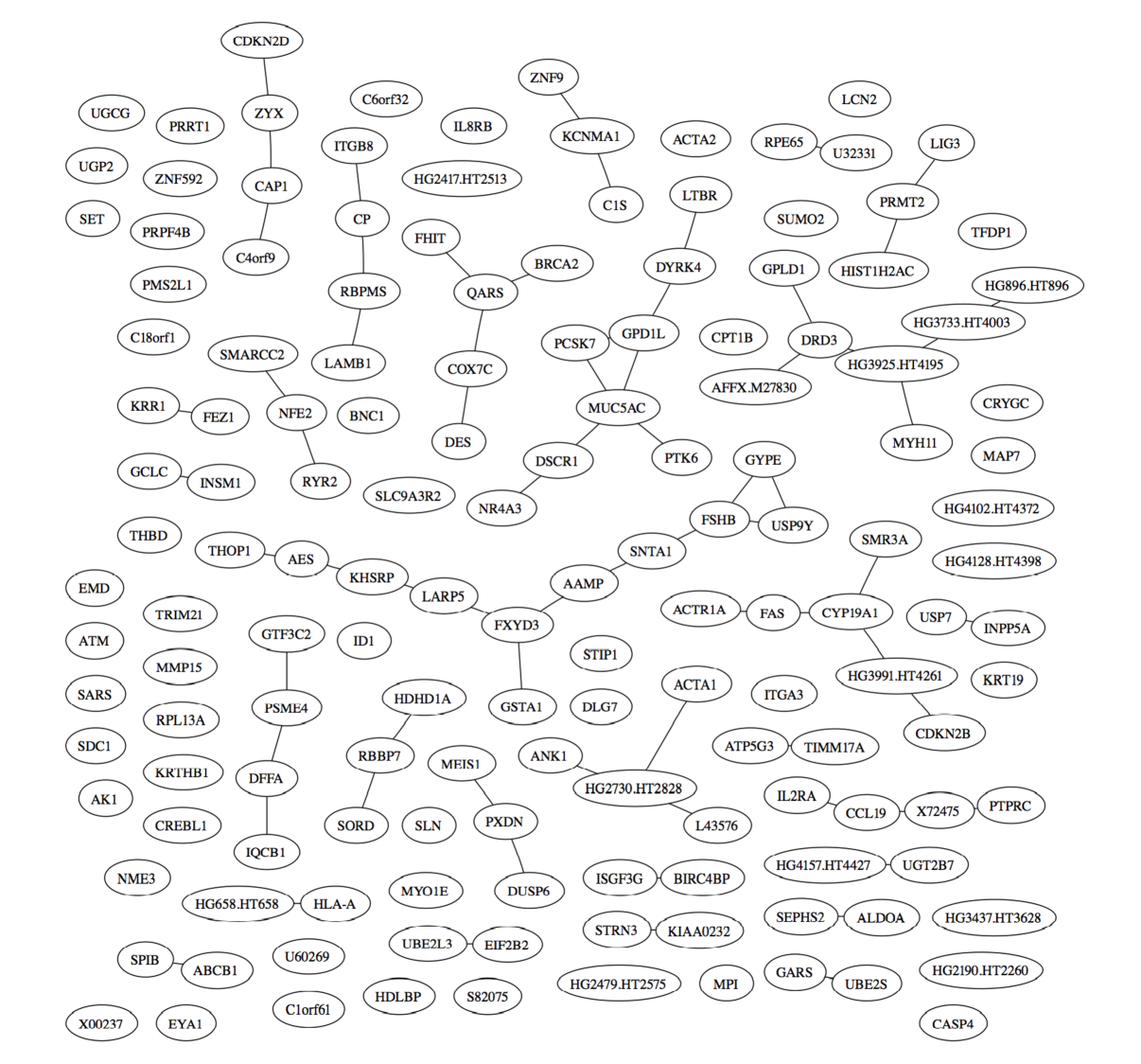
Figure 1. Conditional independence graph for the Schwartz et al. (2002) gene expression data set (random subset of 150 probe sets), based on a sparse shrinkage estimate of the partial correlation matrix. Only the partial correlations with absolute values larger than the $C=50\%$ percentile are considered significantly different from zero and shown as edges. The nodes represent probe sets, which are labelled by the corresponding gene symbols if known, otherwise they are identified by their Affymetrix probe set ID’s.

5. MCMC samplers for the covariate indicator $\boldsymbol{\gamma}$

Based on the dependence structure estimated in the way described above, the covariate indicator vector $\boldsymbol{\gamma}$ in the Bayesian variable selection model could be updated in each MCMC iteration by first selecting a variable at random and then updating this variable and in addition all those in the same neighbourhood, that is the variables which are considered to be related based on the estimated dependence matrix. In a straight-forward implementation of the graph structure described above, one could use all separate sub-graphs as neighbourhoods, which would produce a natural neighbourhood structure. This is especially the case when constructing the graph based on the partial correlations $\rho_{ik}$, since then all nodes (i.e. gene variables), which are not connected through edges, can be considered conditionally independent. However, these conditional independence graphs constructed from gene expression data tend to consist of a few large sub-graphs (neighbourhoods) and many very small neighbourhoods, most of them singletons (see Figure 1 for a small-scale example). This would mean that whenever a gene in one of the largest sub-graphs is selected for sampling, this iteration would take quite long and genes in these sub-graphs would be covered by the MCMC algorithm much more often than genes, which are in small sub-graphs. Based on the results of preliminary test runs where we assessed Markov chain mixing relative to required CPU time, an alternative approach for neighbourhood-building is preferred here: only the direct neighbours of a variable, defined as all nodes to which it is directly connected via an edge in the graph, are considered to be in a neighbourhood with this variable. Note that this implies that there is no fixed structure of non-overlapping neighbourhoods. We have implemented and tried other variations of this neighbourhood approach, in particular the possibility to use not only the first-order neighbours but also a random selection of up to $k$ second-order neighbours. Since preliminary test runs did not yield promising results, this was not pursued further, but the implementation is available in the MATLAB toolbox BVS.

For each MCMC iteration, the elements of $\boldsymbol{\gamma}$ within the selected neighbourhood of variables $i\in\boldsymbol{I}$ are proposed to be updated. This can be done by any MCMC sampler. Here we propose the univariate Gibbs sampler, updating each $\gamma_{i}$ by sampling from its full conditional distribution $p(\gamma_{i}|\boldsymbol{\gamma}_{-i},\boldsymbol{z},\boldsymbol{x},\boldsymbol{\lambda})$. In addition, one can argue that a joint update for all $\gamma_{i}$ ($i\in\boldsymbol{I}$), sampling from the joint conditional distribution $p(\boldsymbol{\gamma}_{I}|\boldsymbol{\gamma}_{-I},\boldsymbol{z},\boldsymbol{x},\boldsymbol{\lambda})$, might be advantageous, especially here, where the variables within a neighbourhood are selected because they are considered to be related. Hence, in the simulation studies in Section 6, the following MCMC algorithms are assessed and compared with respect to mixing and convergence performances relative to CPU time per iteration:

1. Neighbourhood samplers: select $\gamma_{k}$ randomly, find the set of neighbours $nb(k)$ and within neighbourhood $\boldsymbol{I}_{k}=\{k\}\cup nb(k)$ update using:

   1. Univariate Gibbs ($Gibbs$): for each $\gamma_{i}\in\boldsymbol{I}_{k}$ sample from its full conditional distribution $p(\gamma_{i}|\boldsymbol{\gamma}_{-i},\boldsymbol{z},\boldsymbol{x},\boldsymbol{\lambda})$.

   2. Restricted joint Gibbs ($Joint<d>$): for vector $\boldsymbol{\gamma}_{I_{kd}}$ ($\boldsymbol{I}_{kd}\subseteq\boldsymbol{I}_{k}$) sample from joint full conditional distribution $p(\boldsymbol{\gamma}_{I_{kd}}|\boldsymbol{\gamma}_{-I_{kd}},\boldsymbol{z},\boldsymbol{x},\boldsymbol{\lambda})$ . The size of $\boldsymbol{I}_{kd}$ is restricted to $d$ for computational reasons, by randomly sampling $\min(d,\#\boldsymbol{I}_{k})$ variables from the set $\boldsymbol{I}_{k}$, where $\#\boldsymbol{I}_{k}$ denotes the size of $\boldsymbol{I}_{k}$.

   3. Restricted univariate Gibbs ($RGibbs<d>$): like univariate Gibbs, but only considering $\gamma_{i}$ with $i\in\boldsymbol{I}_{kd}$ in order to allow direct comparison with $Joint<d>$.

2. Vanilla samplers for comparison:

   1. Add/delete ($AD$): select one $\gamma_{i}$ at random and propose to change state with a Metropolis-Hastings step

   2. Full Gibbs ($Full$): update the entire vector $(\gamma_{i})_{i=1}^{p}$ in each MCMC iteration by sampling from the respective full conditional distributions $p(\gamma_{i}|\boldsymbol{\gamma}_{-i},\boldsymbol{z},\boldsymbol{x},\boldsymbol{\lambda})$ for all $i=1,...,p$.

5.1. Evaluation of the performance of MCMC algorithms

Our main aim is to improve the mixing performance of MCMC samplers with respect to $\boldsymbol{\gamma}$. The mixing of candidate MCMC samplers is assessed visually by plotting the traces of the model deviance (i.e. $-2\times$ log-likelihood), the current size of the model $p_{\gamma}$, and most importantly the $\boldsymbol{\gamma}$ vector itself. Also, mixing is measured by the effective sample sizes $\mbox{ESS}(\gamma_{i})$ (Neal 1993, Kass et al. 1998) of the indicator variables $\gamma_{i}$. The effective sample size is based on the autocorrelations between MCMC steps and intends to assess to what sample size the observed MCMC sample size would correspond to, in terms of information contained in the sample, if the samples were independent observations from the target distribution rather than highly dependent MCMC samples. For each $\gamma_{i}$ it is defined as

(20) $$\mbox{ESS}(\gamma_{i})=\frac{M}{\tau(\gamma_{i})},$$

where

(21) $$\tau(\gamma_{i})=1+2\sum_{\kappa=1}^{\infty}{\varrho_{\kappa}(\gamma_{i})}$$

is the integrated auto-correlation for estimating $\gamma_{i}$ using the Markov chain, with $\varrho_{\kappa}(\gamma_{i})$ denoting the auto-correlation at lag $\kappa$. This definition is motivated by the fact, that $\tau(\gamma_{i})$ is equal to one iff all auto-correlations $\varrho_{\kappa}(\gamma_{i})$ are equal to zero, that is if the samples were independent. Usually, an MCMC sampler will provide strongly positively correlated samples, resulting in a reduction of $\mbox{ESS}(\gamma_{i})$ compared to the sample size $M$.

The effective sample sizes are estimated using the R package coda (Plummer et al. 2006). In coda, in order to provide robust estimators of the integrated auto-correlation, the Markov chain is viewed as a time series and an autoregressive model $AR(k)$ of order $k$ is fitted, assuming the following relationship between the MCMC sample of $\gamma_{i}$ in iteration $m$ and its $k$ previous MCMC samples:

(22) $$\gamma_{i,m}=\alpha_{i1}\gamma_{i,m-1}+...+\alpha_{ik}\gamma_{i,m-k}+\epsilon_{i,m}.$$

The auto-correlations are then estimated from the fitted $AR(k)$ model and plugged into (21) in order to estimate $\tau(\gamma_{i})$ with $\hat{\tau}(\gamma_{i})=1+2\sum_{\kappa=1}^{k}{\hat{\varrho}_{\kappa}(\gamma_{i})}$. The order $k$ of the autoregressive model is determined via the Akaike Information Criterion. However, the maximum possible order that can be fitted is restricted to $10\log_{10}(M)$, as is suggested by Plummer et al. (2006), to reduce the computational burden as well as reduce the variance of the estimator by removing the small and highly unstable auto-correlation estimates of high lag $\kappa$. Note that the stochastic process $(\epsilon_{i,m})_{m=1}^{M}$ is assumed to be a white-noise process and autoregressive processes are commonly used to model continuous normally distributed data. Hence, the $AR(k)$ process is not completely appropriate for modelling a Markov chain of samples for the binary indicator variable $\gamma_{i}$. However, we are not interested in the autoregressive model itself but rather in using it to estimate the effective sample sizes. For this purpose our approach is found to work well, although in extreme situations $\mbox{ESS}(\gamma_{i})$ can take values which can be counter-intuitive to the understanding of mixing. In particular, for an MCMC sample $(\gamma_{i,m})_{m=1}^{M}$, which consists of $M-1$ entries of value $0$ and one entry $1$, then $\mbox{ESS}(\gamma_{i})=M$, although one might expect a much smaller effective sample size value. In reality, such extreme cases are very rare though. In addition, we use the median as a summary measure to represent the mixing properties of the MCMC chains for the entire $\boldsymbol{\gamma}$ vector, since the median is robust to such outliers. Also note that the effective sample size measures $\mbox{ESS}(\gamma_{i})$ are only used to compare mixing effectiveness of various MCMC samplers which are all applied to the same data set using the same prior specifications. Hence, the same posterior distributions are investigated as target distributions for the MCMC samplers, which ensures that the ESS values of the various MCMC algorithms are comparable.

In large-scale applications such as gene expression microarray data analysis it can happen that the majority of the genes is never selected by an MCMC algorithm sampling from a sparse model, i.e. that $\gamma_{i,m}=0\quad\forall m$ for more than half of the variables. Then, the straightforward $\mbox{median}_{i=1}^{p}\mbox{ESS}(\gamma_{i})$ is zero, because $\mbox{ESS}(\gamma_{i})=0$ for all variables $i$, that were not selected at all during the run of the Markov chain. This makes comparisons of the mixing properties between samplers impossible based on this measure. We hence prefer a weighted mean, averaging over the median of all variables that get selected at least once and the median of those which never get included in the model:

(23) $$\mbox{ESS}^{*}(\boldsymbol{\gamma}) = \frac{\#\boldsymbol{I}_{\gamma}}{p}\times\mbox{median}_{i\in\boldsymbol{I}_{\gamma}}\mbox{ESS}(\gamma_{i})+\frac{p-\#\boldsymbol{I}_{\gamma}}{p}\times\mbox{median}_{i\not\in\boldsymbol{I}_{\gamma}}\mbox{ESS}(\gamma_{i})$$

$$= \frac{\#\boldsymbol{I}_{\gamma}}{p}\times\mbox{median}_{i\in\boldsymbol{I}_{\gamma}}\mbox{ESS}(\gamma_{i}),$$

where $\boldsymbol{I}_{\gamma}:=\{i:(\sum_{m=1}^{M}{\gamma_{i,m}})>0\}$.

There is a trade-off between the mixing performance of a Markov chain and the computational complexity of the MCMC algorithm. Thus, we also compare the ratios $R$ of average effective sample sizes to CPU times $t$ required for the $M$ MCMC iterations after burn-in

(24) $$R(\boldsymbol{\gamma})=\frac{\mbox{ESS}^{*}(\boldsymbol{\gamma})}{t}.$$

Global convergence of the Markov chains to their target distribution is monitored by plotting the traces of univariate summary statistics, in particular model size $p_{\gamma}=\sum_{i=1}^{p}{\gamma_{i}}$ and model deviance $-2\log p(\boldsymbol{y}|\boldsymbol{x},\boldsymbol{\beta})=2\sum_{j=1}^{n}{\log(1+\exp(-y_{j}\boldsymbol{x}^{\prime}_{j}\boldsymbol{\beta}))}$. Also, the trace of the indicator variable vector $\boldsymbol{\gamma}$ is plotted by indicating variables which are included in the model as points; variables which are excluded from the model are not shown. Finally, in simulation studies the plots of marginal posterior probabilities $p(\gamma_{i}|\boldsymbol{x},\boldsymbol{y})$ can be used to check how consistently the “true” model is found by the MCMC sampler.

Since we are mostly interested in finding the most frequently selected models and variables, we focus on regions of high posterior probability regions, while keeping in mind that it is likely that convergence has not yet been reached in low probability tails of the posterior distribution. A bigger problem here is that the posterior distribution is multi-modal because $p>>n$, and that the chains might not have visited all the modes. That is why good mixing and the ability of the chains to move freely is more important here than elusive convergence to the target distribution.

6. Simulation studies

In the following the results of two simulation studies are presented. For both studies, 25 data sets have been simulated according to a scheme specified below. In an initial step, a variety of possible implementations of the neighbourhood sampler (as outlined in Section 5) is applied to two selected data sets only out of all 25 sets. The purpose of these initial runs is to determine whether there are notable differences between the performances of the various neighbourhood sampling implementations and which setting is doing best. In these initial runs the threshold values $C\in\{99\%,97.5\%,95\%,90\%,80\%,60\%\}$ are tested in both simulation scenarios, corresponding to sparse estimated dependence structures where variable pairs are only considered to be related if their pairwise estimated absolute correlation or partial correlation is larger than (or equal to) the $C^{th}$ percentile of all pairwise coefficients. A threshold value of $C=0$ means that all variables are updated in each iteration, i.e. that the full Gibbs sampler is applied. An overview over the MCMC samplers is given in Table 2. The full Gibbs sampler and the neighbourhood sampler with the $Joint10$ updates within neighbourhoods are run for a smaller number of MCMC iterations than all other samplers because these samplers are extremely slow. Note that all Markov chains are started from randomly sampled starting values for all variables, sampled from their prior distributions.

After the initial runs, the neighbourhood samplers which performed best are applied to all simulated data sets to compare these MCMC neighbourhood algorithms with the vanilla samplers, i.e. the add/delete Metropolis-Hastings and full Gibbs algorithms. The add/delete sampler is also applied to all 25 simulated data sets, but the full Gibbs algorithm is only run for 10 out of all 25 data sets in both simulation scenarios because of its extreme CPU time requirements. MCMC iteration numbers are the same as for the initial runs listed in Table 2.

Because the per-iteration running time for the full Gibbs sampler and the $Joint10$ neighbourhood sampler is exceptionally long, these two samplers were run for a shorter total number of iterations and a shorter burn-in period than the other samplers. Global convergence in terms of trace plots for model deviance and model size was achieved well within the chosen burn-in period for all samplers. Inference on mixing and convergence performance was adjusted for differences in run lengths. Throughout, all post-burn-in samples were used for posterior inference and assessment of MCMC performance, i.e. no thinning was performed.

Table 2. MCMC samplers applied in initial runs to two data sets out of all 25 sets in both simulation scenarios.

Label	MCMC sampler		MCMC run length N (burn-in length B)
			Simulation 1	Simulation 2
$AD$	Add/delete Metropolis-Hastings		$200,000$ $(50,000)$	$250,000$ $(50,000)$
$Full$	Gibbs update of all $(\gamma_{i})_{i=1}^{p}$		$90,000$ $(10,000)$	$110,000$ $(10,000)$
	Neighbourhood samplers
	neighbour-hood type	Update within neighbourhood $\boldsymbol{I}$
$Pcor$ $<C>$	partial correlation	Univariate Gibbs update of all $i\in\boldsymbol{I}$	$200,000$ $(50,000)$	$250,000$ $(50,000)$
$Corr$ $<C>$	correlation	Univariate Gibbs update of all $i\in\boldsymbol{I}$	$200,000$ $(50,000)$	$250,000$ $(50,000)$
$Random$ $<C>$	random selection	Univariate Gibbs update of all $i\in\boldsymbol{I}$	not applied	$250,000$ $(50,000)$
$Rgibbs4$	partial correlation	Univariate Gibbs update of subset of $\boldsymbol{I}$ of size 4	$200,000$ $(50,000)$	$250,000$ $(50,000)$
$Joint4$	partial correlation	Joint Gibbs update of subset of $\boldsymbol{I}$ of size 4	$200,000$ $(50,000)$	$250,000$ $(50,000)$
$Rgibbs10$	partial correlation	Univariate Gibbs update of subset of $\boldsymbol{I}$ of size 10	$200,000$ $(50,000)$	$250,000$ $(50,000)$
$Joint10$	partial correlation	Joint Gibbs update of subset of $\boldsymbol{I}$ of size 10	$90,000$ $(10,000)$	$110,000$ $(10,000)$

6.1. Simulation scenario 1: generated covariance structure

6.1.1. Simulation setup

The algorithm in Table 3 is used to simulate 25 data sets $(\boldsymbol{x},\boldsymbol{y})$, so that the input data sets $\boldsymbol{x}$ have $p=500$ variables and $n=100$ samples, where the first $p^{*}=5$ variables $(\boldsymbol{x}_{1},...,\boldsymbol{x}_{5})$ are related to the binary response $\boldsymbol{y}$ via a logistic link. The variables are simulated, in a similar manner to example 4.2 in George and McCulloch (1993), such that there are five blocks of $100$ variables each, with moderately strong positive correlations between the variables within blocks which are induced by adding the same standard normal variable $\boldsymbol{w}$ to $100$ independent standard normals $\boldsymbol{x}^{*}_{1},...,\boldsymbol{x}^{*}_{100}$. In addition, correlation is also introduced between blocks by using the same variables $\boldsymbol{x}^{*}_{1},...,\boldsymbol{x}^{*}_{100}$ for generating the five blocks (but with different variables $\boldsymbol{w}$ added to them). The correlation structure that is imposed by this data-generating scenario is illustrated by triangular image plot of the squared empirical correlation matrix of one example data set in Figure 2. The variables linked to the response, i.e. $\boldsymbol{x}_{1},...,\boldsymbol{x}_{5}$, are all in the same block. They are thus positively correlated with each other and with all other variables in their block. They are also correlated with the first five variables in all subsequent blocks, that is $\boldsymbol{x}_{1}$ with $\boldsymbol{x}_{101},\boldsymbol{x}_{201},\boldsymbol{x}_{301},\mbox{ and }\boldsymbol{x}_{401}$, etc. In such a scenario it is harder for a sampling algorithm to find the correct model with all five true covariates $\boldsymbol{x}_{1},...,\boldsymbol{x}_{5}$ than if they were unrelated.

Table 3. Simulation scenario 1 with generated covariance structure.

  For $j=1,...,n=100$ do .

1. $x^{*}_{1j},...,x^{*}_{qj}\mbox{ iid }\sim N(0,1)$ with $q=100$

2. For $m=0,...,4$ do

   1. $w_{m}\sim N(0,1)$

   2. $x_{(m\times q+i^{*})j}=x^{*}_{i^{*}j}+w_{m}$ ($i^{*}=1,...,q$)

3. $y_{j}\sim\mbox{Bernoulli}\left(\frac{\exp(\boldsymbol{x}_{j}\boldsymbol{\beta})}{1+\exp(\boldsymbol{x}_{j}\boldsymbol{\beta})}\right)$, with vectors $\boldsymbol{\beta}=(2,2,2,2,2,0,...,0)$ and $\boldsymbol{x}_{j}=(x_{1j},...,x_{pj}$ have length $p=500$.

 

The Bayesian logistic variable selection model outlined in Section 2 is fitted to each of the 25 data sets $(\boldsymbol{x},\boldsymbol{y})$. Based on the convergence and mixing performances observed in the first two data sets, and as shown in the following, the $Pcor90$ sampler was chosen, i.e. the neighbourhood sampler based on the partial correlation matrix with threshold $C=90\%$. The prior parameter $c^{2}$ in the independence prior distribution $p(\boldsymbol{\beta})=N(\boldsymbol{0}_{p_{\gamma}},c^{2}\boldsymbol{I}_{p_{\gamma}})$ was set to $c^{2}=5$ to guarantee a good coverage of the range of values expected for $\boldsymbol{\beta}$. The prior probability for $\gamma_{i}=1$ was set to $\pi_{i}=p^{*}/p=0.01$ so that the prior expected number of selected variables is equivalent to the true number $p^{*}=5$.

Figure 2. Squared empirical correlation structure imposed on data set 1 in simulation scenario 1.

6.1.2. Markov chain mixing performance

Figure 3 shows the traces of model deviance and model size $p_{\gamma}$ for the add/delete, $Pcor90$, and full Gibbs ($Full$) samplers for simulated data set number 1. As expected, mixing is much slower for the add/delete sampler than for the neighbourhood ($Pcor90$) and full Gibbs samplers. In particular this is also the case for the $\boldsymbol{\gamma}$ vector, where for the add/delete sampler the trace plot shows long “lines”, where points are plotted for each iteration over a long period (where a variable stays in the model for a long time), and equivalently long stretches of no plotted points (where variables are not included for a long time). This is confirmed when measuring the mixing performances of the three samplers in terms of the effective sample sizes $\mbox{ESS}^{*}(\boldsymbol{\gamma})$ (see Tables 4 and 5).

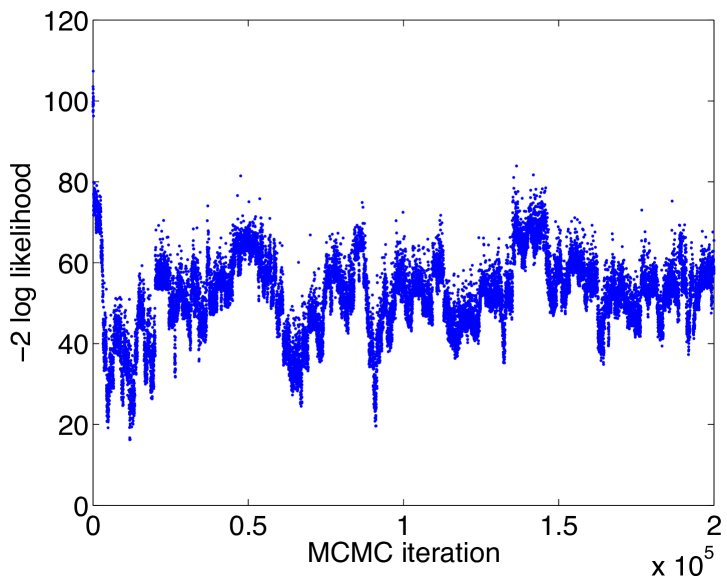
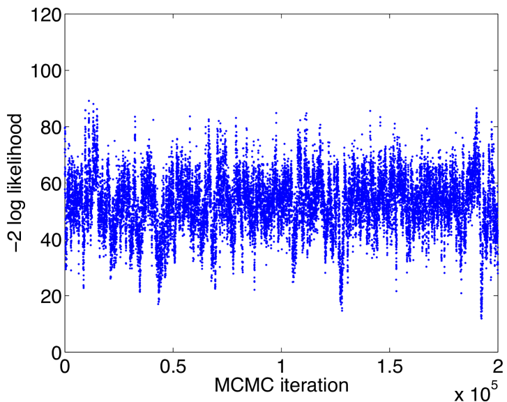
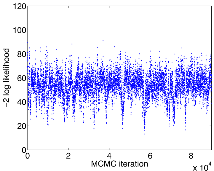
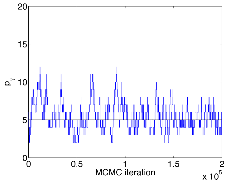
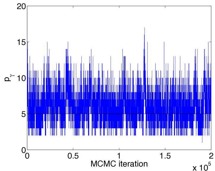
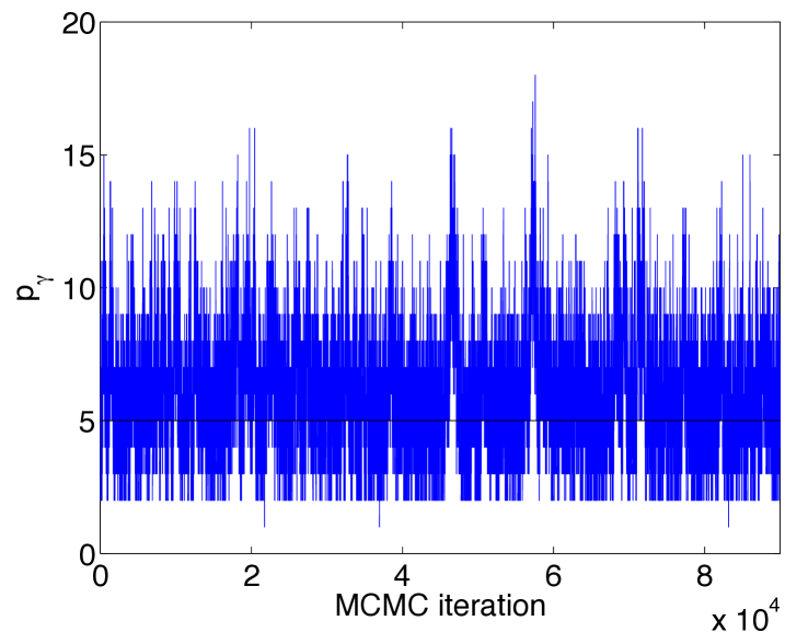
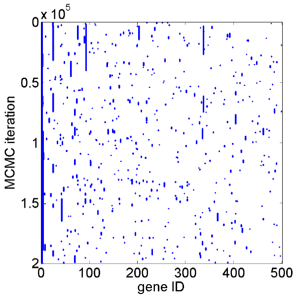
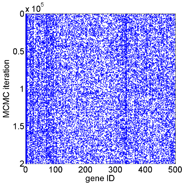
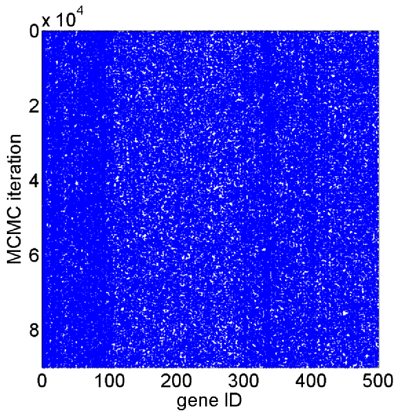
Figure 3. Trace plots of global parameters model deviance (top) and model size $p_{\gamma}$ (middle), as well as trace plots of $\boldsymbol{\gamma}$ vector (bottom) for add/delete sampler (left), one neighbourhood sampler ($Pcor90$) (centre), and for the full Gibbs sampler (right) for data set 1 in scenario 1.

Table 4. Mixing performance results with respect to $\boldsymbol{\gamma}$ for scenario 1 over all 25 data sets (10 data sets for $Full$ sampler, respectively): median values and inter-quartile ranges.

MCMC	CPU time	$\mbox{ESS}^{*}(\boldsymbol{\gamma})$	$R(\boldsymbol{\gamma})$	$\#\boldsymbol{I}^{\sharp}$	# FP†	# FN†
sampler	$t$ (min)
$AD$	38	59	1.58	267	10	1
	(38, 38)	(55, 65)	(1.45, 1.72)	(263, 271)	(8, 14)	(1, 2)
$Pcor90$	168	3024	18.28	500	7	1
	(166, 169)	(2699, 3345)	(16.13, 20.11)	(500, 500)	(5, 12)	(0, 1)
$Full{\ddagger}$	672	10780	17.63	500	8	1
	(664, 676)	(7791, 13700)	(16.07, 21.52)	(500, 500)	(4.5, 10.75)	(0.25, 2)
‡ For $Full$ it is $M=80,000$, compared to $M=150,000$ for all other samplers
♯ $\boldsymbol{I}=\{i:(\sum_{m=1}^{M}{\gamma_{i,m}})>0\}$, i.e. number of variables for which $\gamma_{i}=1$ in at least one MCMC iteration
†false positives and false negatives if cut-off at ratio of posterior to prior probability $>5$, i.e. if
$\hat{p}(\gamma_{i}=1|\boldsymbol{x},\boldsymbol{y})>0.05$

We adjust for the computation time by computing the ratios $R(\boldsymbol{\gamma})$ of effective sample sizes and computation times. These ratios, relative to the ratio $R_{Full}(\boldsymbol{\gamma})$ observed for the full Gibbs algorithm applied to the same data set, are displayed in the left-hand side plot in Figure 4 for all neighbourhood samplers for the first two simulated data sets. In addition, the values $R_{Pcor90}(\boldsymbol{\gamma})$ are shown for the $Pcor90$ samplers applied to all 10 generated data sets for which the full Gibbs sampler was run. The $Pcor90$ sampler is chosen for computation in all data sets and for comparison with the full Gibbs and add/delete samplers, because the comparison of a range of threshold sizes in the first two data sets indicates, that the $90\%$ percentile is within the range of threshold values $C$, for which the neighbourhood samplers are at their highest efficiency in terms of effective sample size per CPU time (see Figure 4 and Table 5). The right-hand side of Figure 4 shows the evolution of computation times (per $10,000$ MCMC samples) for the neighbourhood samplers with increasing neighbourhood sizes.

The effective sample size relative to CPU time $R(\boldsymbol{\gamma})$ is larger for all neighbourhood samplers than for the add/delete sampler and increases with decreasing threshold level (corresponding to larger average neighbourhood sizes). It is also larger than the value for the full Gibbs sampler, for all but the smallest neighbourhood sizes. There is no obvious difference between the neighbourhood samplers constructed using partial correlations and those built from estimated correlation matrices. All $R_{Pcor90}(\boldsymbol{\gamma})/R_{Full}(\boldsymbol{\gamma})$ ratios (for those ten data sets for which $R_{Full}(\boldsymbol{\gamma})$ is available) are larger than one, implicating that in this simulation scenario the $Pcor90$ sampler leads to larger effective sample sizes relative to CPU time requirements than the full Gibbs sampler.

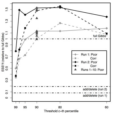
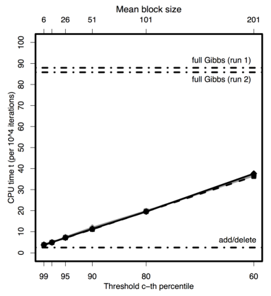
Figure 4. Ratio of effective sample size and CPU time $R(\boldsymbol{\gamma})=\mbox{ESS}^{*}(\boldsymbol{\gamma})/t$ (left), and CPU times per $10^{4}$ iterations (min) (right), plotted against the threshold level $C$ for the neighbourhood samplers for data sets 1 and 2 in simulation setup 1. In addition, for threshold $C=0.9$, $R(\boldsymbol{\gamma})$ is plotted for simulated data sets 1 to 10.

The results for all 25 generated data sets are summarised in Table 4. The median of the $R_{Pcor90}(\boldsymbol{\gamma})$ values $\mbox{median}_{k=1}^{10}{R_{Pcor90}(\boldsymbol{\gamma})}=18.28$ is slightly larger than the median of the full Gibbs values $R_{Full}(\boldsymbol{\gamma})$, which is equal to $\mbox{median}_{k=1}^{25}{R_{Full}(\boldsymbol{\gamma})}=17.63$, and although the inter-quartile ranges overlap, we have seen from Figure 4 that for each pairwise comparison within a generated data set it is $R_{Pcor90}(\boldsymbol{\gamma})>R_{Full}(\boldsymbol{\gamma})$.

An additional indicator of Markov chain mixing, particularly in a high-dimensional setting, is the proportion of all variables that are visited by the Markov chain at least once. While the add/delete algorithm only visited 265 of all 500 variables in the application to simulated data set 1 (see Table 5), this number is larger for all neighbourhood samplers and increases with decreasing threshold values $C$. Comparing the $Pcor$ and $Corr$ samplers with the smallest average neighbourhood sizes, i.e. with the largest values of $C$, the partial-correlation based samplers visit more variables than the corresponding correlation based neighbourhood samplers.

6.1.3. Posterior variable inclusion probabilities

Figure 5 shows the medians and inter-quartile ranges of the MCMC estimates of the posterior variable inclusion probabilities $\hat{p}(\gamma_{i}=1|\boldsymbol{x},\boldsymbol{y})$ for variables $\boldsymbol{x}_{1},...,\boldsymbol{x}_{10}$, over all 25 generated data sets. These include the $p^{*}=5$ “true” predictors $(\boldsymbol{x}_{1},...,\boldsymbol{x}_{5})$ which were generated as being linked to the response variable $\boldsymbol{y}$. In particular, the individual plots in Figure 5 illustrate the evolution of the MCMC estimates $\hat{p}(\gamma_{i}=1|\boldsymbol{x},\boldsymbol{y})$, when the number of post-burn-in MCMC iterations $M$ increases. The results shown for variables $\boldsymbol{x}_{6},...,\boldsymbol{x}_{10}$ are representative of the posterior inclusion probability estimates that we find for all variables which are simulated not to be linked to the response $\boldsymbol{y}$. As expected, the median posterior inclusion probability estimates of these variables are close to zero for all values of $M$ and both samplers, with very small associated inter-quartile ranges. Because in the add/delete sampler individual variables are visited and proposed for a state change so rarely, even after $M=10,000$ post-burn-in iterations the median posterior inclusion frequencies are still either zero or very close to one for the five “true” predictors. Only after all $M=150,000$ iterations do the add/delete sampler median values of the estimates start to move away from the extreme values at which they were fixed simply due to slow mixing of the Markov chain. The $Pcor90$ sampler does not have this problem, with median values of the estimates being different from the extremes zero and one even for $M=1,000$ iterations. In fact, for all $M\in\{1000,10000,50000,150000\}$ the median posterior inclusion frequencies are similar, with inter-quartile ranges becoming narrower with increasing sample sizes, reflecting a convergence to the true posterior variable inclusion probabilities $p(\gamma_{i}=1|\boldsymbol{x},\boldsymbol{y})$ on the level of the individual generated data sets. Overall, the inter-quartile ranges are narrower for the neighbourhood sampler than for the add/delete sampler.

Note that the median values of the estimated posterior inclusion probabilities are considerably smaller than one, and in fact converge to values between around 0.2 and 0.4 with increasing MCMC run lengths. In individual data sets, on average one of the five variables has even an estimated posterior inclusion probability smaller than 0.05. These cases are labelled as false negative in Tables 4 and 5. This is linked to the fact that in individual data sets, other variables ($\boldsymbol{x}_{i}$ with $i\in\{6,...,500\}$) are sometimes found to have high posterior inclusion probability estimates. These variables are counted as false positive in the tables, again using a cut-off at $\hat{p}(\gamma_{i}=1|\boldsymbol{x},\boldsymbol{y})>0.05$. These results can be explained by mixing or convergence problems of the MCMC algorithm, but also by the presence of multi-collinearity in the input data matrix $\boldsymbol{x}$ which necessarily arises when the number of variables $p$ is larger than the sample size $n$.

$M=1000$

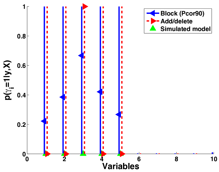
$M=10000$

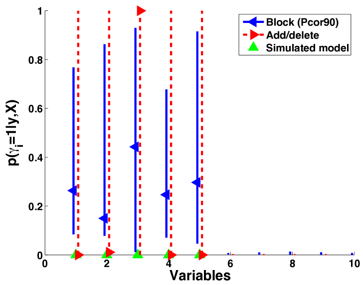
$M=50000$

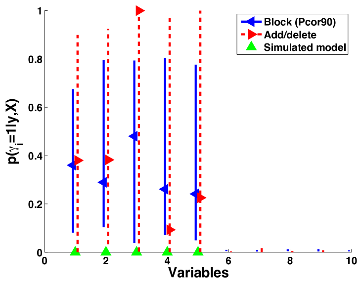
$M=150000$

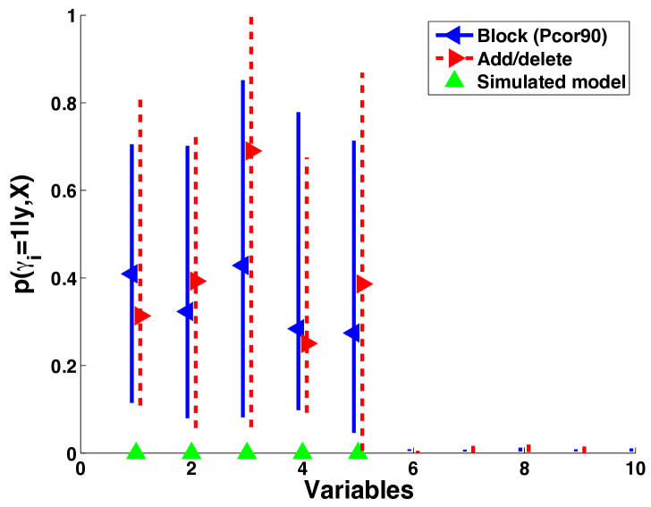
Figure 5. Posterior inclusion frequencies (median and inter-quartile ranges) for variables $1,...,10$ over all 25 replicates of simulation setup 1 (after burn-in period).

6.1.4. Alternative Gibbs updates within the neighbourhoods

As part of this simulation study, we apply multivariate Gibbs sampling with $d\in\{4,10\}$ (denoted $Joint4$ and $Joint10$) to two of the generated data sets for both simulation scenarios. For comparison with regards to computing times we also apply the corresponding restricted univariate Gibbs samplers $Rgibbs4$ and $Rgibbs10$, where the maximum possible number of variables to be updated within an MCMC iteration is also restricted to $\min(\#\boldsymbol{I},d)$ with $d\in\{4,10\}$. For all these samplers, the $Pcor90$ mechanism is used to determine the underlying neighbourhood structure, because the above comparison of neighbourhood samplers with different threshold sizes $C$ has indicated that the $Pcor90$ sampler performs well in terms of the ratio of effective sample size and computation time.

Table 5. Mixing performance results with respect to $\boldsymbol{\gamma}$ for scenario 1: results for one data set (run 1).

MCMC	CPU time	$\mbox{ESS}^{*}(\boldsymbol{\gamma})$	$R(\boldsymbol{\gamma})$	$\#\boldsymbol{I}^{\sharp}$	# FP†	# FN†
sampler	$t$ (min)
$AD$	40	65	1.65	265	7	1
$Full^{\ddagger}$	704	13910	19.77	500	7	1
Neighbourhood sampler
$Pcor99$	56	558	9.88	484	12	1
$Pcor97.5$	74	1193	16.06	497	10	1
$Pcor95$	107	2094	19.57	500	10	1
$Pcor90$	170	3802	22.39	500	7	1
$Pcor80$	293	6559	22.39	500	8	1
$Pcor60$	564	13160	23.34	500	7	1
$Corr99$	56	380	6.80	411	14	1
$Corr97.5$	74	967	13.07	481	8	1
$Corr95$	107	1528	14.33	499	9	1
$Corr90$	166	3309	19.89	500	9	1
$Corr80$	293	7357	25.07	500	8	1
$Corr60$	544	11580	21.27	500	7	1
$Rgibbs4$	56	298	5.29	463	12	1
$Joint4$	88	354	4.03	455	10	0
$Rgibbs10$	71	971	13.64	499	7	1
$Joint10^{\ddagger}$	1423	620	0.44	474	10	1
‡ For $Full$ and $Joint10$ it is $M=80,000$, compared to $M=150,000$ for all other samplers
♯ $\boldsymbol{I}=\{i:(\sum_{m=1}^{M}{\gamma_{i,m}})>0\}$, i.e. number of variables for which $\gamma_{i}=1$ in at least one MCMC iteration
†false positives and false negatives if cut-off at ratio of posterior to prior probability $>5$, i.e. if
$\hat{p}(\gamma_{i}=1|\boldsymbol{x},\boldsymbol{y})>0.05$

The results for one data set of simulation scenario 1 are summarised in Table 5. While the computation time needed for the $Joint4$ run is with 88 minutes only about half the time needed for the univariate Gibbs run ($Pcor90$), the time required to run the $Joint10$ sampler explodes to nearly 24 hours for only $N_{Joint10}=90,000$ MCMC iterations in contrast to $N_{Pcor90}=200,000$ iterations. At the same time, the effective sample sizes $\mbox{ESS}^{*}(\boldsymbol{\gamma})$ are only $9\%$ of $\mbox{ESS}^{*}_{Pcor90}(\boldsymbol{\gamma})$ for the $Joint4$ sampler, and only $31\%$ for the $Joint10$ algorithm when adjusting for the differences in post-burn-in MCMC run lengths ($M_{Pcor90}=150,000$ vs. $M_{Joint10}=80,000$) by assuming a linear relationship between $\mbox{ESS}^{*}(\boldsymbol{\gamma})$ and $M$. Thus, with increasing set sizes $d$ in multivariate-Gibbs-within-neighbourhood samplers $Joint<d>$, the required computation time seems to increase too quickly and to outweigh the improvement achieved in mixing as measured by $\mbox{ESS}^{*}(\boldsymbol{\gamma})$. Also, the effective sample sizes of the multivariate samplers are only modestly larger than those of their corresponding restricted univariate Gibbs samplers ($Rgibbs4$ and $Rgibbs10$): the ratios of the effective sample sizes are about $1.2$ for both $d=4$ and $d=10$, again when adjusting $\mbox{ESS}^{*}_{Joint10}(\boldsymbol{\gamma})$ for the reduced post-burn-in MCMC run length.

We conclude that joint moves, which update a fixed number of variables $d$ jointly, are by themselves not a useful sampling strategy. However, it might be useful to include such updates in a portfolio of moves, if there are covariates which are strongly correlated. Such a flexible sampler, which could select updating moves randomly from a portfolio of possible updates, might benefit from occasional joint updates of strongly correlated covariates.

6.2. Simulation scenario 2: covariance based on gene expression data

6.2.1. Simulation setup

In this second simulation scenario (see Table 6) we use a real gene expression data set (Schwartz et al. 2002) to generate the covariance structure between variables. For that purpose, $p=500$ variables are selected at random from all $7129$ probe sets available in the ovarian cancer gene expression data set provided by Schwartz et al. (2002). This data set is described in more detail and analysed in Section 7. It contains $n=104$ samples which are used for generating the simulated data sets. Again, 25 data sets $(\boldsymbol{x},\boldsymbol{y})$ are generated, so that the first $p^{*}=5$ variables $(\boldsymbol{x}_{1},...,\boldsymbol{x}_{5})$ are related to the binary response $\boldsymbol{y}$ via a logistic link. The natural correlation structure among the 500 randomly selected variables is illustrated by the triangular image plot of the squared empirical correlation matrix of one of the 25 generated data sets in Figure 6. Pairwise empirical correlations range from $-0.7$ to $0.9$. Again, the prior parameter $c^{2}$ in the independence prior distribution $p(\boldsymbol{\beta})=N(\boldsymbol{0}_{p_{\gamma}},c^{2}\boldsymbol{I}_{p_{\gamma}})$ is set to $c^{2}=5$. The prior probability for $\gamma_{i}=1$ is set to $\pi_{i}=p^{*}/p=0.01$.

Table 6. Simulation scenario 2 based on gene expression data by Schwartz et al. (2002).

 

1. $\boldsymbol{x}$ (input matrix of dimension $n\times p$): select $p=500$ gene variables at random from pre-processed and normalised gene expression microarray data set $\tilde{x}$ of dimension $\tilde{p}\times n=7129\times 104$ by Schwartz et al. (2002) (described in Section 7), standardise all variables to have zero mean and unit variance.

2. For $j=1,...,n=104$ do
   $y_{j}\sim\mbox{Bernoulli}\left(\frac{\exp(\boldsymbol{x}_{j}\boldsymbol{\beta})}{1+\exp(\boldsymbol{x}_{j}\boldsymbol{\beta})}\right)$, with vector $\boldsymbol{\beta}=(2,2,2,2,2,0,...,0)$ of length $p=500$ and $\boldsymbol{x}_{j}$ ($j=1,...,n$) denoting the column vectors of $\boldsymbol{x}$.

 

Figure 6. Squared empirical correlation structure of one data set simulated according to simulation scenario 2.

6.2.2. Markov chain mixing performance

We follow the structure of analysis outlined for the simulation scenario 1 in the previous section. Figure 7 shows the trace plots of model deviance (top) and model size (middle) and the individual traces for all $\gamma_{i}$ with $i=1,...,500$ (bottom) for the add/delete Metropolis-Hastings sampler, the $Pcor90$ sampler and the full Gibbs algorithm for one generated data set. The conclusions are much the same as for simulation scenario 1, that is mixing with respect to sampling $\boldsymbol{\gamma}$ is much slower for the add/delete sampler than for the $Pcor90$ and full Gibbs algorithms. In addition, there is also an obvious improvement in mixing for the full Gibbs sampler compared to the neighbourhood sampler, when viewing the trace plots of $\boldsymbol{\gamma}$. In terms of the effective sample sizes $\mbox{ESS}^{*}(\boldsymbol{\gamma})$ (see Table 8 for the results for data set 1), values increase about 40-fold for the neighbourhood sampler compared to add/delete algorithm and more than 220-fold for the full Gibbs sampler after adjustment for the reduced post-burn-in run length $M_{Full}=100,000$ (compared to $M_{AD}=M_{Pcor90}=200,000$), which is a slightly smaller improvement than what we had observed in simulation scenario 1.

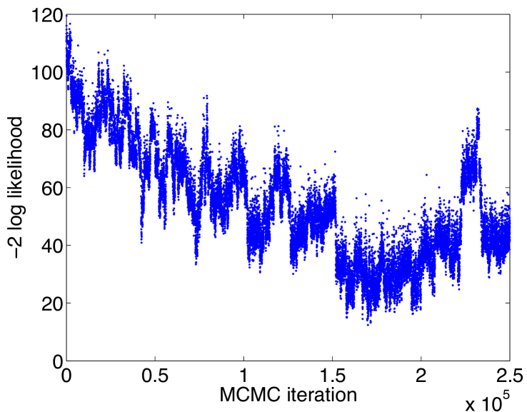
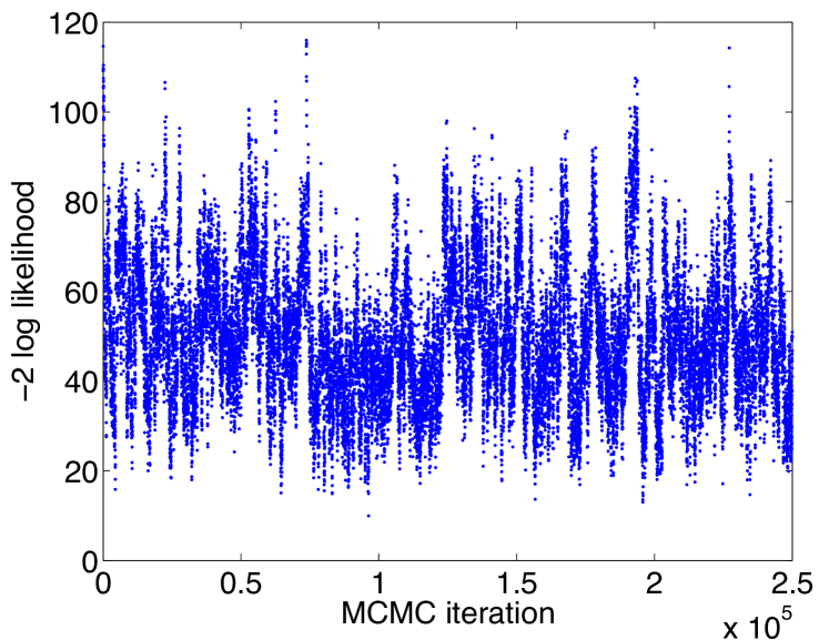
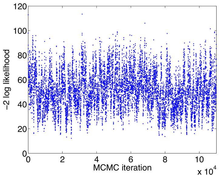
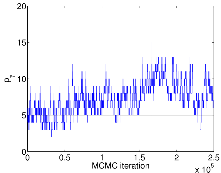
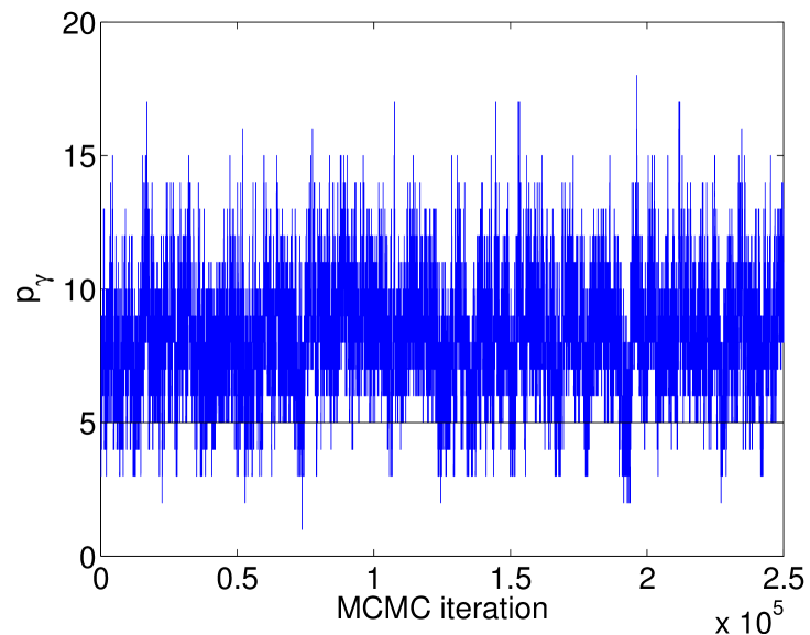
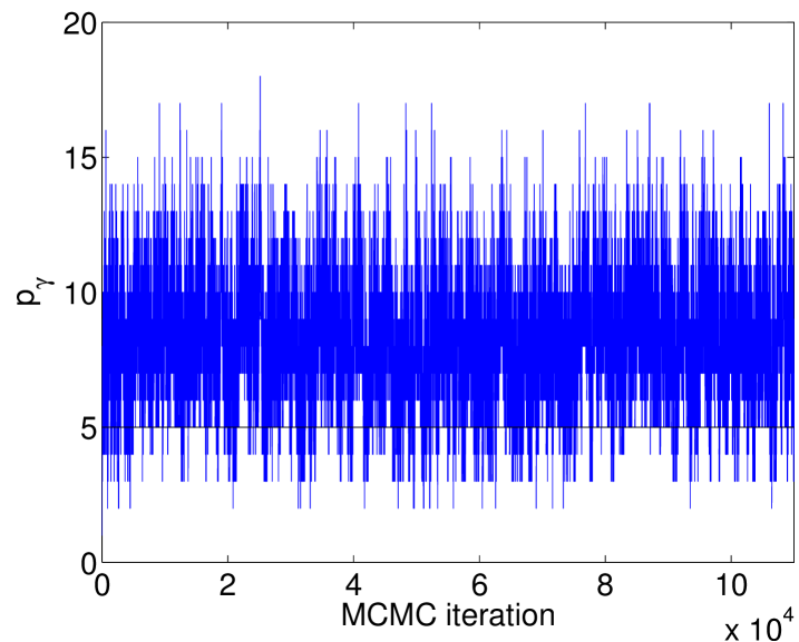
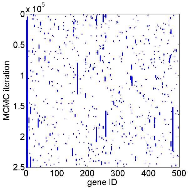
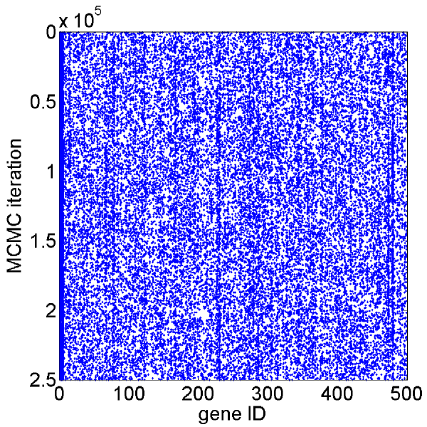
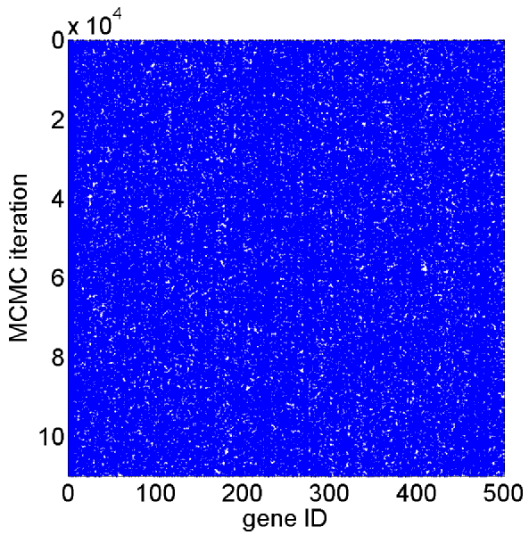
Figure 7. Trace plots of global parameters model deviance (top) and model size $p_{\gamma}$ (middle), as well as trace plots of $\boldsymbol{\gamma}$ vector (bottom) for add/delete sampler (left), one neighbourhood sampler ($Pcor90$) (centre), and for the full Gibbs sampler (right) for data set 1 in scenario 2.

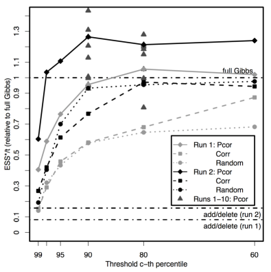
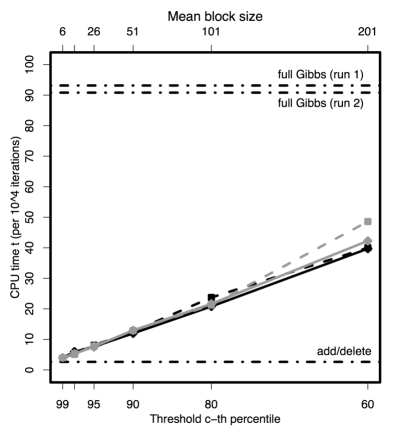
Figure 8. Ratio of effective sample size and CPU time $R(\boldsymbol{\gamma})=\mbox{ESS}^{*}(\boldsymbol{\gamma})/t$ (left), and CPU times per $10^{4}$ iterations (min) (right), plotted against the threshold level $C$ for the neighbourhood samplers for data sets 1 and 2 in scenario 2. In addition, for thresholds $C=0.9$ and $C=0.8$, $R(\boldsymbol{\gamma})$ is plotted for simulated data sets 1 to 10.

The ratios $R(\boldsymbol{\gamma})$ of effective sample sizes and computation times, relative to the ratio $R_{Full}(\boldsymbol{\gamma})$ for the full Gibbs algorithm, are displayed in the left-hand side plot in Figure 8 for all neighbourhood samplers for the first two simulated data sets. Also, the ratios $R_{Pcor90}(\boldsymbol{\gamma})/R_{Full}(\boldsymbol{\gamma})$ and $R_{Pcor80}(\boldsymbol{\gamma})/R_{Full}(\boldsymbol{\gamma})$ are shown for the $Pcor90$ and $Pcor80$ samplers applied to those 10 generated data sets for which the full Gibbs sampler has been run. As before, the right-hand side of Figure 8 shows the linear evolution of computation times (per $10,000$ MCMC samples) for the neighbourhood samplers with increasing neighbourhood sizes.

The effective sample sizes relative to CPU time $R(\boldsymbol{\gamma})$ are larger for all neighbourhood samplers than for the add/delete sampler and increase with decreasing threshold level (corresponding to larger average neighbourhood sizes), until levelling off between $C=0.9$ and $C=0.8$. Contrary to simulation scenario 1, the partial-correlation based neighbourhood samplers now have considerably larger effective sample sizes and hence larger values of $R(\boldsymbol{\gamma})$ than the samplers using correlation estimates for neighbourhood construction. In fact, now the $Corr$ samplers do not outperform the full Gibbs sampler in terms of $R(\boldsymbol{\gamma})$ for the two displayed data sets, while the $Pcor$ algorithms do result in better mixing than full Gibbs sampling if the threshold is large enough. Seven out of ten $R_{Pcor90}(\boldsymbol{\gamma})/R_{Full}(\boldsymbol{\gamma})$ ratios, for which $R_{Full}(\boldsymbol{\gamma})$ is available, are larger than one.

Table 7. Mixing performance results with respect to $\boldsymbol{\gamma}$ for scenario 2 over all 25 data sets (10 data sets for $Full$ sampler, respectively): median values and inter-quartile ranges.

MCMC	CPU time	$\mbox{ESS}^{*}(\boldsymbol{\gamma})$	$R(\boldsymbol{\gamma})$	$\#\boldsymbol{I}^{\sharp}$	# FP†	# FN†
sampler	$t$ (min)
$AD$	53	103	1.96	316	10	1
	(53, 53)	(100, 105)	(1.88, 1.99)	(303, 321)	(6, 15)	(0, 2)
Neighbourhood	241	5148	21.46	500	8	0
($Pcor90$)	(239, 243)	(4773, 6000)	(20.11, 24.89)	(500, 500)	(4, 9)	(0, 1)
$Full^{\ddagger}$	931	16690	17.94	500	9	0
	(928, 932)	(12320, 23170)	(13.20, 25.00)	(500, 500)	(5, 9.75)	(0, 2)
‡ For $Full$ it is $M=100,000$, compared to $M=200,000$ for all other samplers
♯ $\boldsymbol{I}=\{i:(\sum_{m=1}^{M}{\gamma_{i,m}})>0\}$, i.e. number of variables for which $\gamma_{i}=1$ in at least one MCMC iteration
†false positives and false negatives if cut-off at ratio of posterior to prior probability $>5$, i.e. if
$\hat{p}(\gamma_{i}=1|\boldsymbol{x},\boldsymbol{y})>0.05$

The results for all 25 generated data sets are summarised in Table 7. The median of the $R_{Pcor90}(\boldsymbol{\gamma})$ values $\mbox{median}_{k=1}^{25}{R_{Pcor90}(\boldsymbol{\gamma})}=21.46$ is larger than the median of the full Gibbs values $R_{Full}(\boldsymbol{\gamma})$ $\mbox{median}_{k=1}^{10}{R_{Full}(\boldsymbol{\gamma})}=17.94$, although again the inter-quartile ranges overlap.

In terms of the number of variables visited by the MCMC algorithms, the picture is the same as for simulation scenario 1. While the add/delete algorithm only visited 323 of all 500 variables at least once in the application to simulated data set 1 (see Table 8), this number is larger for all neighbourhood samplers and increases with decreasing threshold values $C$. Comparing the $Pcor$ and $Corr$ samplers with large thresholds $C$, the partial-correlation based samplers visit more variables than the correlation based neighbourhood samplers.

6.2.3. Posterior variable inclusion probabilities

Figure 9 shows the median values and inter-quartile ranges of the MCMC estimates of the posterior variable inclusion probabilities $\hat{p}(\gamma_{i}=1|\boldsymbol{x},\boldsymbol{y})$ for variables $(\boldsymbol{x}_{1},...,\boldsymbol{x}_{10})$, over all 25 generated data sets. These include the $p^{*}=5$ “true” predictors $(\boldsymbol{x}_{1},...,\boldsymbol{x}_{5})$, which were generated as being linked to the response variable $\boldsymbol{y}$. The results shown for variables $(\boldsymbol{x}_{6},...,\boldsymbol{x}_{10})$ are representative for all variables, which are simulated not to be correlated with the response $\boldsymbol{y}$, and again, the median posterior inclusion probability estimates of these variables are close to zero for all values of $M$ and both samplers. After $M=200,000$ post-burn-in iterations the median estimates for the five “true” predictors for the neighbourhood sampler converge at values of around 0.8. Overall, the inter-quartile ranges are again narrower for the neighbourhood sampler than for the add/delete sampler, but seem to be wider after $M=200,000$ than in simulation scenario 1 after $M=150,000$ iterations. The median values of the estimated posterior inclusion probabilities are between about 0.7 and 0.9 for the neighbourhood sampler and between 0.3 and 0.9 for the add/delete algorithm at $M=200,000$. In individual data sets, the median number of false negatives is zero for the neighbourhood and full Gibbs samplers, but one for the add/delete algorithm (Tables 7 and 8). The median numbers of false positives range from 8 ($Pcor90$) to 10 ($AD$), when using the same cut-off as that used for marking the false negatives, at $\hat{p}(\gamma_{i}=1|\boldsymbol{x},\boldsymbol{y})>0.05$.

$M=1000$

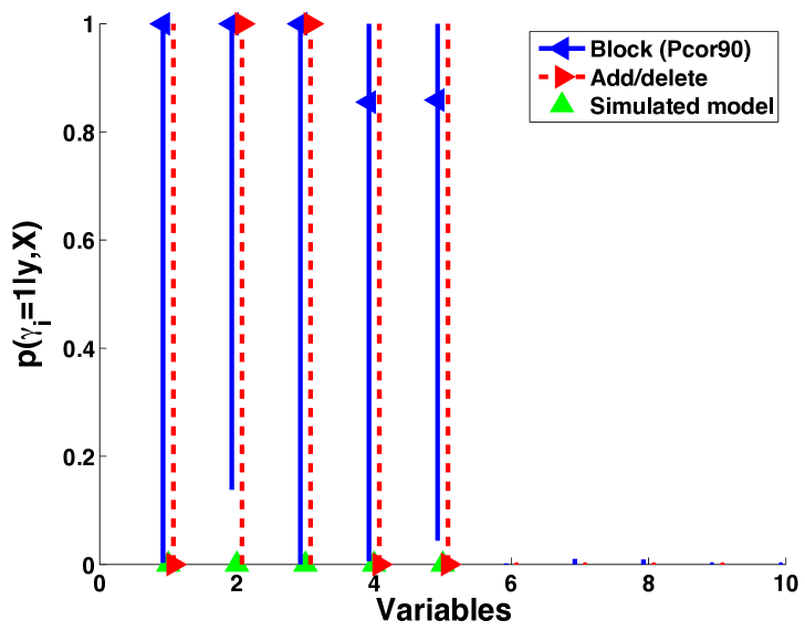
$M=10000$

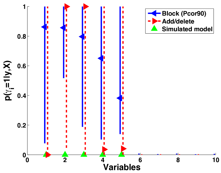
$M=50000$

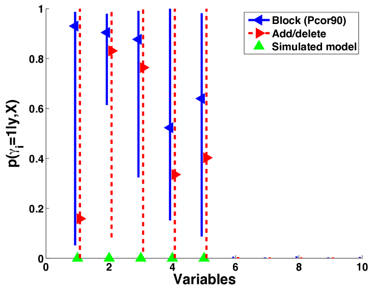
$M=200000$

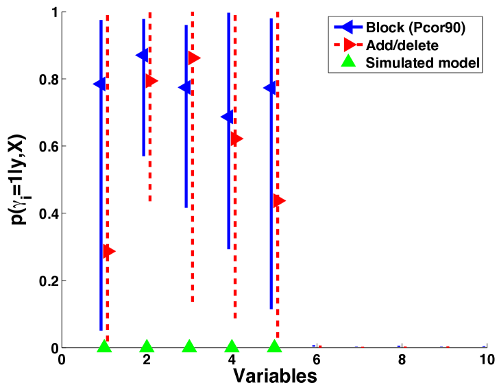
Figure 9. Posterior inclusion frequencies (median and inter-quartile ranges) for variables $1,...,10$ over all 25 replicates of simulation setup 2 (after burn-in period).

6.2.4. Alternative Gibbs samplers within the neighbourhoods

We again apply the restricted joint Gibbs samplers $Joint4$ and $Joint10$, and in addition the corresponding restricted univariate Gibbs samplers $Rgibbs4$ and $Rgibbs10$. Again, the $Pcor90$ mechanism is used to determine the underlying neighbourhood structure. The results of data set 1 of simulation scenario 2 are summarised in Table 8. While the computation time needed for the $Joint4$ run is with 112 minutes less than half the time needed for the univariate Gibbs run ($Pcor90$), the time required to run the $Joint10$ sampler is 30 hours for only $N_{Joint10}=110,000$ MCMC iterations instead of $N_{Pcor90}=250,000$ iterations. At the same time, the effective sample sizes $\mbox{ESS}^{*}(\boldsymbol{\gamma})$ are only $11\%$ of $\mbox{ESS}^{*}_{Pcor90}(\boldsymbol{\gamma})$ for the $Joint4$ sampler, and only $30\%$ for the $Joint10$ algorithm when adjusting for the differences in post-burn-in MCMC run lengths ($M_{Pcor90}=200,000$ vs. $M_{Joint10}=100,000$). We draw the same conclusions as before, i.e. that any improvement in mixing with increasing set sizes $d$ in multivariate-Gibbs-within-neighbourhood samplers $Joint<d>$ is outweighed by the exponentially increasing computation time. Also, the effective sample sizes of the multivariate samplers are only modestly larger than those of their corresponding restricted univariate Gibbs samplers ($Rgibbs4$ and $Rgibbs10$), with ratios of the effective sample sizes being about $1.1$ for both $d=4$ and $d=10$ (when adjusting $\mbox{ESS}^{*}_{Joint10}(\boldsymbol{\gamma})$ for the reduced post-burn-in MCMC run length).

6.2.5. Random construction of neighbourhoods

In addition to neighbourhoods constructed by means of estimated correlation and partial correlation matrices, for comparison reasons we here also construct neighbourhoods simply by randomly drawing variables into neighbourhoods, matching the neighbourhood sizes with the mean sizes observed for the partial-correlation-based and correlation-based neighbourhood structures for the given threshold values $C$. These $Random<C>$ neighbourhood samplers are applied to the first two of the 25 generated data sets. The results for data set 1 are listed in Table 8, and the curves of the ratios $R_{Random}(\boldsymbol{\gamma})$ values relative to $R_{Full}(\boldsymbol{\gamma})$ are shown in Figure 8. The effective sample sizes and consequently the ratios $R(\boldsymbol{\gamma})=\mbox{ESS}^{*}(\boldsymbol{\gamma})/t$ of the $Random<C>$ samplers are similar to the $Corr<C>$ samplers for the two observed data sets. This suggests that for this simulation scenario, where the correlation structure of the data corresponds to that of a real gene expression data set, the $Corr<C>$ samplers are not doing better in terms of mixing relative to computation time than neighbourhood samplers with the same mean neighbourhood sizes, where the “neighbourhoods” are just random selections of genes. The $Pcor<C>$ samplers, on the other hand, are consistently more efficient than the $Random<C>$ samplers. These observations conform with the idea that the dependence structure in gene expression data can better be explained by a sparse partial correlation structure than by a sparse correlation matrix, i.e. that the sparsity is observed in terms of conditional dependence rather than marginal dependence.

Table 8. Mixing performance results with respect to $\boldsymbol{\gamma}$ for scenario 2: results for one data set (run 1). Diagnostic measures for Markov chain mixing with respect to $\boldsymbol{\gamma}$.

MCMC	CPU time	$\mbox{ESS}^{*}(\boldsymbol{\gamma})$	$R(\boldsymbol{\gamma})$	$\#\boldsymbol{I}^{\sharp}$	# FP†	# FN†
sampler	$t$ (min)
$AD$	53	104	1.96	323	14	0
$Full^{\ddagger}$	932	11640	12.50	500	10	0
Neighbourhood sampler
$Pcor99$	82	618	7.54	473	11	0
$Pcor97.5$	108	1399	12.94	491	14	0
$Pcor95$	153	2120	13.84	499	12	0
$Pcor90$	259	4090	15.80	500	11	0
$Pcor80$	433	6564	15.16	500	9	0
$Pcor60$	845	13100	15.49	500	11	0
$Corr99$	80	268	3.35	377	11	1
$Corr97.5$	109	574	5.26	422	12	0
$Corr95$	156	1196	7.67	463	12	0
$Corr90$	258	2473	9.59	494	11	0
$Corr80$	425	5163	12.14	500	10	0
$Corr60$	972	11460	11.79	500	13	0
$Random99$	77	187	2.41	498	13	0
$Random97.5$	109	554	5.07	500	12	0
$Random95$	153	1340	8.75	500	13	0
$Random90$	247	2877	11.65	500	10	0
$Random80$	457	5447	11.92	500	11	0
$Random60$	846	10312	12.20	500	13	0
$Rgibbs4$	75	412	5.53	479	11	0
$Joint4$	112	448	3.98	482	8	0
$Rgibbs10$	94	1099	11.67	499	8	0
$Joint10^{\ddagger}$	1777	611	0.34	485	12	0
‡ For $Full$ and $Joint10$ it is $M=100,000$, compared to $M=200,000$ for all other samplers
♯ $\boldsymbol{I}=\{i:(\sum_{m=1}^{M}{\gamma_{i,m}})>0\}$, i.e. number of variables for which $\gamma_{i}=1$ in at least one MCMC iteration
†false positives and false negatives if cut-off at ratio of posterior to prior probability $>5$, i.e. if
$\hat{p}(\gamma_{i}=1|\boldsymbol{x},\boldsymbol{y})>0.05$

6.3. Sensitivity analysis for prior variance parameter $c^{2}$

Throughout this section, the covariance parameter $c^{2}$ in $\boldsymbol{\beta}\sim N(\boldsymbol{0}_{p},c^{2}\boldsymbol{I}_{p})$ was set to 5. This value was chosen to provide a relatively flat prior across the expected range coefficient values, and in particular to comfortably include the “true” regression coefficient values $\beta_{1}=...=\beta_{5}=2$, which were used to simulate the five covariates that are linked to the response. To see, how much this choice of $c^{2}=5$ has influenced the posterior distributions, not just of $\boldsymbol{\beta}$, but also of the main parameter of interest $\boldsymbol{\gamma}$, a range of different values for $c^{2}$ has been applied in this section. Both the add/delete and $Pcor90$ samplers have been applied to one of the data sets generated according to simulation scenario 2.

In several previous publications, where the probit model was used for variable selection in binary regression rather than the logistic model (e.g. Brown et al. 1998b, Lee et al. 2003, Tadesse et al. 2005), the authors had warned that the posterior inference about the covariate indicator variable $\boldsymbol{\gamma}$ can be influenced by the choice of the prior covariance parameter $c^{2}$. For g-priors, i.e. $\boldsymbol{\beta}\sim N(\boldsymbol{0}_{p},c^{2}(\boldsymbol{x}^{\prime}\boldsymbol{x})^{-1})$, the suggestion by Smith and Kohn (1996) to use large values of $c^{2}$ ranging between 10 and 100 is often followed. For the independence prior, which is used here, Brown et al. (2002) and Sha et al. (2004) suggest values which are small relative to typically expected regression coefficient values $\boldsymbol{\beta}$ and are chosen in order to allow for good inference about $\boldsymbol{\gamma}$ (rather than $\boldsymbol{\beta}$). In particular, Sha et al. (2004) argue for using a value $c^{2}$ which implies a ratio of prior to posterior precision of between 0.1 and 0.005. The prior precision is $1/c^{2}$ for all variables $\boldsymbol{x}_{i}$ and the posterior precision is $1/c^{2}+e_{i}$ where the vector $(e_{i})_{i=1,...,n-1}$ of eigenvalues of the precision matrix is equal to the inverse of the vector of non-zero eigenvalues of the empirical covariance matrix. Consequently, the range of $c^{2}$ is given by

(25) $$c(\bar{e},0.1)<c^{2}<c(\bar{e},0.005),$$

where $c(e,p)=(1-p)/(pe)$ and $\bar{e}$ denotes the mean eigenvalue. This criterion is proposed for data matrices where the condition number, i.e. the ratio of maximum and minimum eigenvalues, is not too large.

We use the simulation scenario 2 to compare the sensitivity of both, probit and logistic, BVS regression models with regards to the influence of $c^{2}$ on Markov chain mixing and convergence behaviour, and posterior inference about $\boldsymbol{\gamma}$ and $\boldsymbol{\beta}$. The probit regression model is implemented in the auxiliary variable formulation described by Albert and Chib (1993) as given in equation (3). We apply the MCMC sampling algorithms for Bayesian probit regression detailed in Holmes and Held (2006).

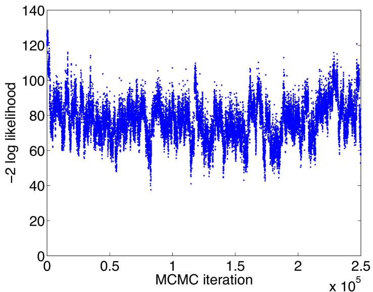
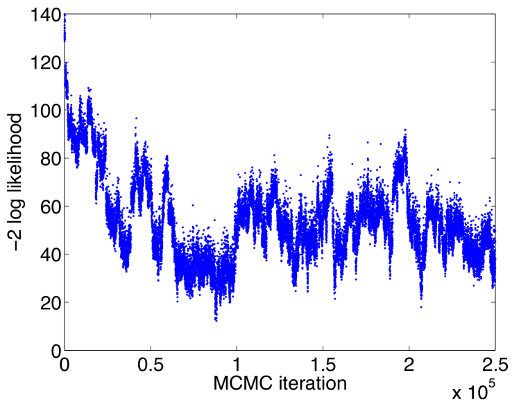
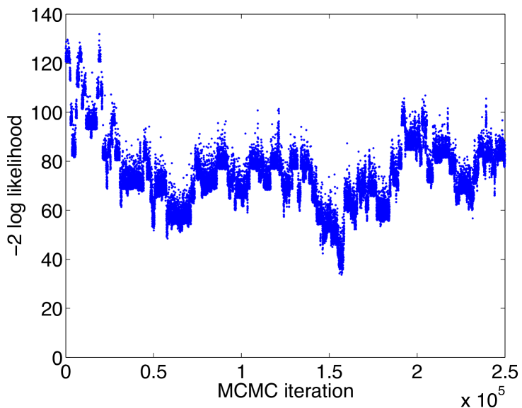
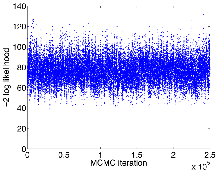
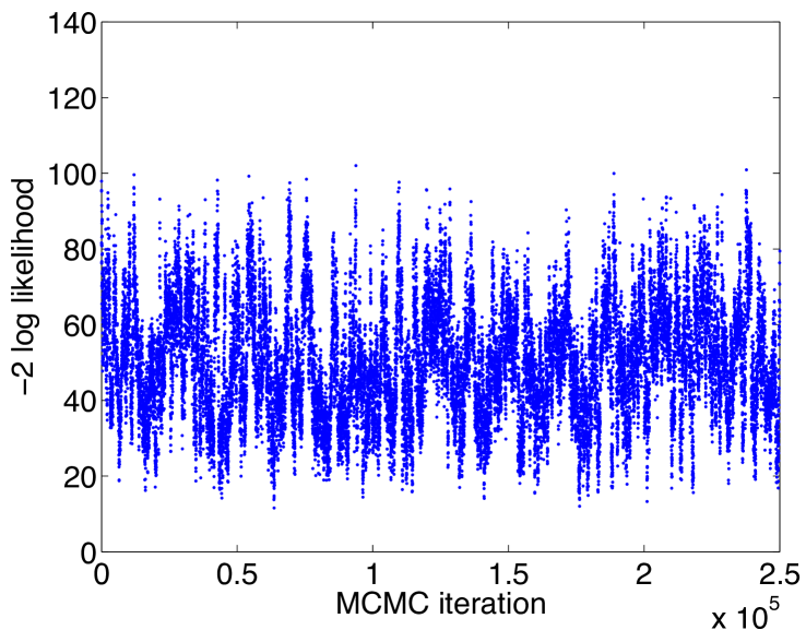
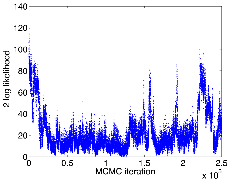
Figure 10. Logistic BVS model: trace plots of model deviance for add/delete samplers (top) and neighbourhood samplers ($Pcor90$) (bottom) with prior covariance parameters $c^{2}=0.5$ (left), $c^{2}=5$ (centre, standard value chosen throughout simulation studies in previous section), and $c^{2}=50$ (right).

Starting with the logistic variable selection model, the trace plots of the model deviances in Figure 10 are used to visually monitor MCMC convergence and mixing. In terms of model deviance, the Markov chains mix better and converge faster, if the prior covariance parameter $c^{2}$ is chosen to be small, for both add/delete and neighbourhood sampling algorithms. This is also true for chain mixing at the level of the individual covariate indicators $\boldsymbol{\gamma}$ as indicated by the effective sample sizes $\mbox{ESS}^{*}$ and the numbers of variables $\#\boldsymbol{I}$ visited by the chains at least once (see Table 9). This behaviour is not unexpected, since decreasing the size of $c^{2}$ restricts the posterior parameter space so that it is easier for Markov chains to cover the entire posterior distribution and find the regions of high density quickly. Note that in the logistic variable selection model, for all choices of $c^{2}\in\{0.5,5,50\}$ Markov chains generated by the $Pcor90$ sampler mix better than the corresponding add/delete Metropolis-Hastings Markov chains.

In addition to monitoring the mixing and convergence properties of the Markov chains, we also look at the posterior mean estimates of $\boldsymbol{\beta}_{\gamma}$ and $\boldsymbol{\gamma}$. Remember that the “true” underlying vector of regression coefficients used to simulate the data set is $\boldsymbol{\beta}=(2,2,2,2,2,0,...,0)$ and the “true” value of $\boldsymbol{\beta}_{\gamma}$ for the model defined by $\boldsymbol{\gamma}=(1,1,1,1,1,0,...,0)$ would be $\boldsymbol{\beta}_{\gamma}=(2,2,2,2,2)$. So in Table 9, the estimates $\boldsymbol{\hat{\beta}}_{\gamma}$ from the posterior distribution are summarised in terms of the ranges (minimum and maximum values) of the variables $\beta_{1},...,\beta_{5}$ on the one hand, and of $\beta_{6},...,\beta_{500}$ on the other hand. While we expect the estimates of the former to be close to the value two, the latter should vary around zero. Indeed, the estimates $\hat{\beta}_{\gamma i}$ for $i=6,...,500$ vary around zero, with the ranges becoming larger with increasing values of $c^{2}$. The values of $\hat{\beta}_{\gamma i}$ for $i=1,...,5$ also depend on the choice of $c^{2}$, with those posterior estimates obtained with the prior covariance paramater $c^{2}=5$ being closest to the expected value 2 (although being slightly too large with ranges of $(2.13,3.03)$ for the add/delete sampler and $(2.22,3.16)$ for the neighbourhood sampler). Note that the $\hat{\beta}_{\gamma i}$ are the marginal estimates computed by averaging over all MCMC iterations after burn-in $m=1,...,M$, where $\gamma_{i,m}=1$, not taking into account, which other variables are included in the model at each iteration. Hence, the estimates are not conditioned to the “true” model, where $\boldsymbol{\gamma}=(1,1,1,1,1,0,...,0)$. More important for the variable selection problem is posterior inference about the covariate indicator vector $\boldsymbol{\gamma}$. The results for $\boldsymbol{\gamma}$ are summarised in terms of false positives and false negatives, defined using the threshold $\hat{p}(\gamma_{i}=1|\boldsymbol{x},\boldsymbol{y})>0.05$ as before in this manuscript. The add/delete sampler with $c^{2}=50$ is the only MCMC run, where not all five “true” predictors are detected at that level, with variable 3 never even having been visited by the Markov chain. There is no obvious difference in the numbers of false positives selected by the samplers at other values of $c^{2}$. In summary, the logistic variable selection model is quite robust to the choice of the prior covariance parameter $c^{2}$ in terms the covariate indicator vector $\boldsymbol{\gamma}$. This allows to use the samplers for inference about variable selection and model selection without need for fine-tuning $c^{2}$.

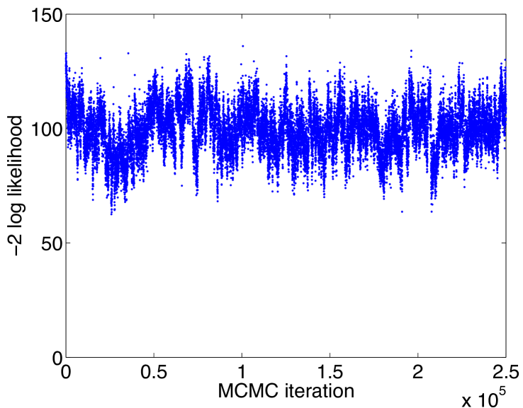
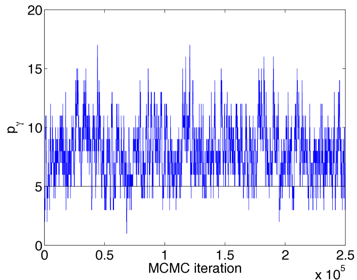
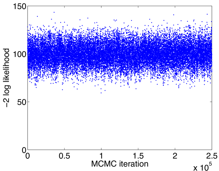
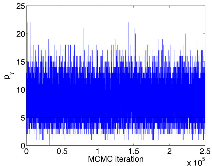
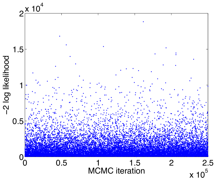
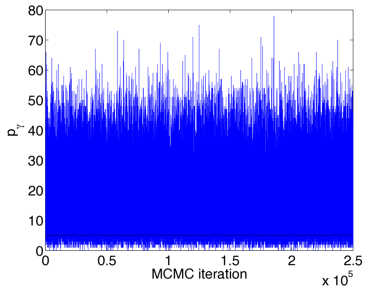
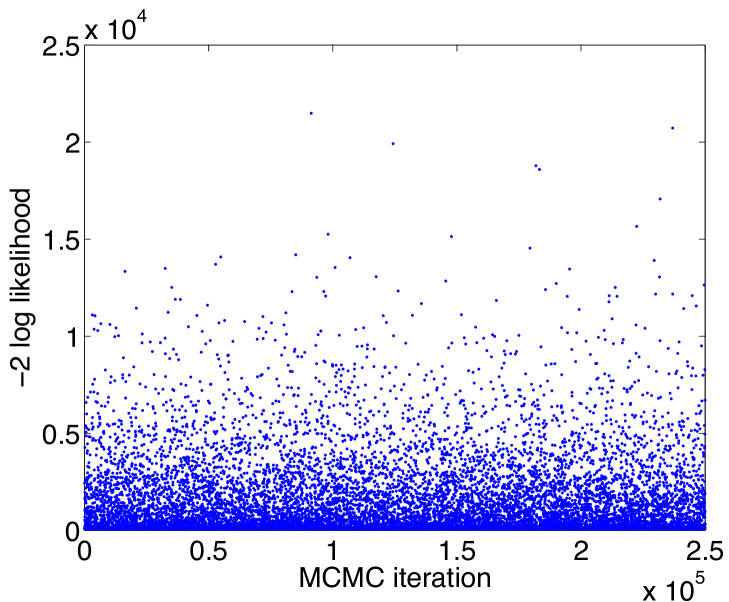
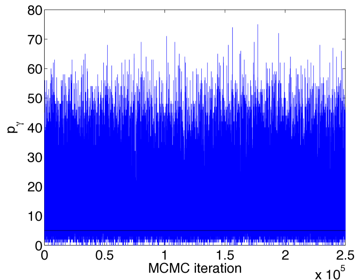
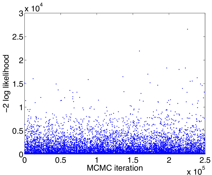
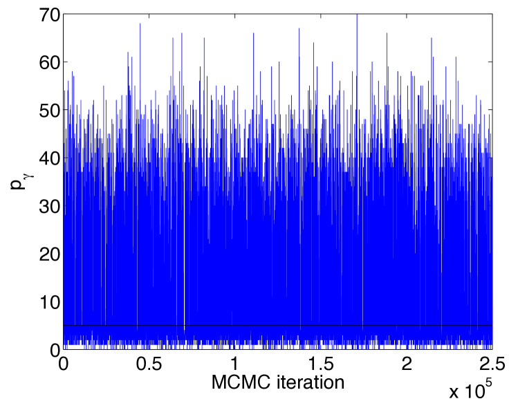
Figure 11. Probit BVS model: trace plots of model deviances (left) and model sizes (right) for add/delete sampler with prior covariance parameter $c^{2}=0.05$ and neighbourhood samplers ($Pcor90$) with $c^{2}=\{0.05,0.5,5,50\}$ (from top to bottom).

The probit variable selection model is much more sensitive to the choice of $c^{2}$, especially the add/delete algorithm, which does not even converge if $c^{2}$ is chosen too large (see Table 9). Instead, the samplers start to include more and more variables until the number of variables in the model became larger than the sample size $n=104$. Consequently, the samplers slow down significantly, due to the necessity to invert large matrices of size $k\times k$ with $k=\min(p_{\gamma},n)$ in every iteration. At that point, the sampling process was stopped manually due to convergence problems. This problem is related to the fact, that in sparse situations with small variable inclusion probability $\pi=p^{*}/p$, the acceptance probability for deleting variables tends to zero with $\pi\to 0$ in the add/delete Metropolis-Hastings algorithm. This in turn means that the algorithm proposes to add variables much more often than to delete variables, leading to the sampler running off to include more and more variables. In our simulation runs the convergence problem could only be avoided by choosing a very small prior covariance parameter value of $c^{2}=0.05$, which then resulted in very small posterior mean estimates $\hat{\beta}_{\gamma i}$, but good posterior inference on the probabilities $\hat{p}(\gamma_{i}=1|\boldsymbol{x},\boldsymbol{y})>0.05$ for variable inclusion (see Table 9). Incidentally, $c^{2}=0.05$ does not fit within the range of values suggested by Sha et al. (2004), as the values in equation (25) correspond to the range $3.33<c^{2}<73.70$ for the data set used in this example. Contrary to the add/delete algorithm, the Gibbs sampler using $Pcor90$ neighbourhoods does not break down, if a large $c^{2}$ is chosen. However, the trace plots of the model size $p_{\gamma}$ (Figure 11) illustrate that large models are often visited with many more variables being included than in the logistic variable selection models with the same value of $c^{2}$. In addition, the model deviance trace plots shown in Figure 11 indicate that the sampler frequently moves into regions of low posterior probability, and the posterior mean estimates of $\boldsymbol{\beta}_{\gamma}$ run off to extreme values with magnitudes up to $10^{12}$ for $c^{2}=50$ (Table 9). However, the posterior inference about variable inclusion probabilities $p(\gamma_{i}=1|\boldsymbol{x},\boldsymbol{y})$ is still quite robust, as reflected by the number of false negatives and false positives (Table 9). Most samplers still find all five “true” predictor variables, but the number of false positives is slightly larger than was observed for the corresponding logistic models for some values of $c^{2}$, in particular for $c^{2}=0.5$. One could circumvent this problem of having to fine-tune $c^{2}$ in a probit BVS model by introducing a hyper-prior distribution for $c^{2}$. For the g-prior $c^{2}(\boldsymbol{x}^{\prime}\boldsymbol{x})^{-1}$ possible hyper-prior implementations $p(c^{2})$ have for example been presented by Bottolo and Richardson (2010).

Finally, in terms of the binomial prior distribution $p(\gamma_{i})=\pi_{i}$ ($i=1,...,p$), it should be mentioned that our strategy to choose the prior so that all $\pi_{i}$ correspond to the expected fraction of true predictors among all variables, might not be the best strategy, if the main interest lies in finding the “true” predictors rather than the overall “true” model. In that situation, choosing a binomial prior probability $\pi_{i}$, which is larger than the expected proportion $p^{*}/p$, would mean that the models which are visited by the Markov chain will tend to be larger than the expected size $p^{*}$, which will increase the chance that all “true” variables of interest will be included in that model.

Table 9. Results of sensitivity analysis regarding the choice of $c^{2}$. MCMC samplers are evaluated on data set 1 in simulation scenario 2.

$c^{2}$	abort due to	$(\min\hat{\beta}_{\gamma i},\max\hat{\beta}_{\gamma i})$	$(\min\hat{\beta}_{\gamma i},\max\hat{\beta}_{\gamma i})^{\ddagger}$	# FP†	# FN†	$\mbox{ESS}^{*}(\boldsymbol{\gamma})$	$\#\boldsymbol{I}^{\sharp}$
	convergence	for $i=1,...,5$	for $i=6,...,500$
	problems?
Logistic BVS model
Add/delete sampler
0.5	no	(0.92, 1.52)	(-0.85, 0.87)	13	0	177	437
5	no	(2.13, 3.03)	(-2.34, 1.88)	15	0	84	330
50	no	(1.61, 3.51)♭	(-1.42, 1.88)	10	2	46	147
Neighbourhood sampler ($Pcor90$, univariate Gibbs within neighbourhoods)
0.5	no	(0.89, 1.49)	(-0.83, 0.92)	14	0	8699	500
5	no	(2.22, 3.16)	(-1.82, 1.96)	12	0	4195	500
50	no	(4.59, 8.95)	(-4.90, 5.65)	18	0	1629	500
Probit BVS model
Add/delete sampler
0.05	no	(0.36, 0.60)	(-0.39, 0.42)	11	0	185	478
0.5	yes	N/A	N/A	N/A	N/A	N/A	N/A
5	yes	N/A	N/A	N/A	N/A	N/A	N/A
50	yes	N/A	N/A	N/A	N/A	N/A	N/A
Neighbourhood sampler ($Pcor90$, univariate Gibbs within neighbourhoods)
0.05	no	(0.35, 0.60)	(-0.38, 0.43)	14	0	10020	500
0.5	no	(103.38, 6.00$e4$)	(-5.64$e5$, 1.09$e9$)	49	0	9116	500
5	no	(2815.56, 1.59$e8$)	(-1.42$e9$, 2.02$e12$)	25	0	8873	500
50	no	(236.82, 4.13$e5$)	(-6.60$e10$, 2.17$e12$)	13	1	8246	500
♯ $\boldsymbol{I}=\{i:(\sum_{m=1}^{M}{\gamma_{i,m}})>0\}$, i.e. number of variables for which $\gamma_{i}=1$ in at least one MCMC iteration
†false positives and false negatives if cut-off at ratio of posterior to prior $>5$ (i.e. $\hat{p}(\gamma_{i}=1|\boldsymbol{x},\boldsymbol{y})>0.05$)
‡only for variables, which were visited at least once by the Markov chain
♭does not include $\beta_{\gamma 3}$, which was never visited by the Markov chain
♮N/A = not applicable

7. Application to ovarian cancer gene expression data

We apply the Bayesian variable selection logistic model to an ovarian cancer gene expression data set (Schwartz et al. 2002) in order to classify between intrinsically chemotherapy-resistant tumours and more responsive histologies. The gene expression data were generated by Affymetrix HuGeneFL gene chips which contain 7129 probe sets, each corresponding to a specific gene. Here, $p=4000$ of these gene variables are used after univariate unspecific filtering. Data are available for $n=104$ ovarian cancer tissue samples, including 18 mucinous and clear-cell samples, which are inherently resistant against the standard platinum-based chemotherapeutic drug, while the 86 serous and endometrioid tumours are usually more responsive to treatment. The microarray data are background-correction by the RMA procedure (Irizarry et al. 2003) and loess-normalised within each array(Cleveland 1979). In addition, all gene variables are centred and scaled to have zero mean and unit variance. In the Bayesian logistic variable selection model the sparsity-inducing hyper-parameters are set to the values $\pi_{i}=5/p=0.00125$ for all $i=1...,p$, so that $5$ variables are expected to be selected a priori. The value $c^{2}=10$ is larger than in the simulation examples in Section 6 to account for the fact that now the true $\beta_{i}$ values are unknown and not set within the range $[-2,2]$, as it was the case with the simulation data.

We compare the performances of four MCMC algorithms for sampling from the logistic BVS model: the vanilla add/delete Metropolis-Hastings sampler, a neighbourhood MCMC sampler (Pcor, C=99%) and in addition both samplers in combination with a parallel tempering algorithm. Parallel tempering is implemented such that only neighbouring Markov chains in the temperature ladder are proposed for state swaps in a Metropolis-Hastings algorithm. We use five parallel Markov chains and a geometric temperature ladder $\{1,\tau,\tau^{2},\tau^{3},\tau^{4}\}$ with $\tau=1.2$. All parallel Markov chains are run un-coupled, i.e. without state swaps, for $B^{PT}=50,000$ iterations before starting the parallel tempering algorithm proper to allow the Markov chains to move towards their target distribution before starting exchange moves between chains. An alternative approach could be the all-exchange parallel tempering scheme by Calvo (2005), where all possible pairwise swap acceptance probabilities are computed for all parallel chains in each iteration and the pair of chains, that is to be swapped, is sampled according to this probability distribution. Both algorithms have been implemented in the MATLAB toolbox BVS available from http://www.bgx.org.uk/software.html. Results are compared with our previous analysis based on lasso logistic regression (Tibshirani 1996), where five genes were found to be especially strongly linked to the response (Zucknick et al. 2008). Between one (untempered $AD$) and four (both MCMC runs with parallel tempering) of these genes are recovered here (see Table 10).

Table 10. Diagnostic measures for Markov chain mixing with respect to $\boldsymbol{\gamma}$; results for $M=1,000,000$ post burn-in MCMC iterations (CPU time for total iteration number $N=1,100,000$).

MCMC	CPU time	$\mbox{ESS}^{*}(\boldsymbol{\gamma})$	$\#\boldsymbol{I}^{\sharp}$	# genes	# genes not
sampler	$t$ (min)			in lasso†	in lasso‡
$AD$	315	8	198	1	23
$Pcor99$	1356	3,793	2856	3	6
Parallel tempering
with $AD$	1726	19,900	1091	4	15
with $Pcor99$	6601	41,985	3752	4	5
${}^{\sharp}\boldsymbol{I}=\{i:(\sum_{m=1}^{M}{\gamma_{i,m}})>0\}$
†How many of the five genes consistently selected by lasso in (Zucknick et al. 2008) are
recovered by BVS, if cut-off at posterior to prior prob. $>10$, i.e. $\hat{p}(\gamma_{i}=1|\boldsymbol{x},\boldsymbol{y})>0.0125$?
‡How many genes are consistently selected besides these five genes (Zucknick et al. 2008)?

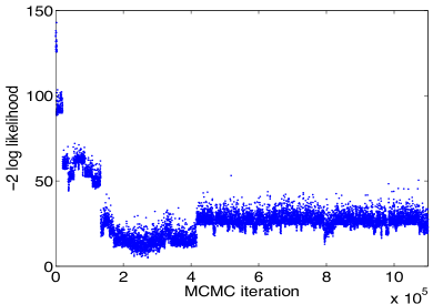
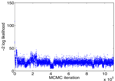
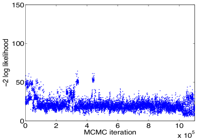
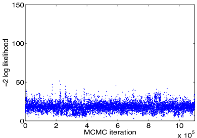
Figure 12. Trace plots of model fit in terms of model deviances for add/delete sampler (left) and neighbourhood sampler (Pcor99) (right), with (bottom) and without (top) parallel tempering in application to gene expression data (Schwartz et al. 2002).

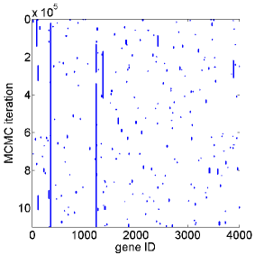
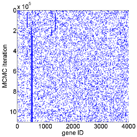
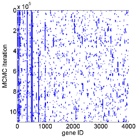
Figure 13. Trace plots of $\boldsymbol{\gamma}$ vector for add/delete sampler (left) and neighbourhood sampler (Pcor99) (right), with (bottom) and without (top) parallel tempering in application to gene expression data (Schwartz et al. 2002).

The add/delete sampler gets stuck with a model that has a worse fit in terms of model deviance than many other models (Figure 12). This model consistently contains two variables with IDs 354 (gene symbol ANX4) and 1232 (TFF1), so that overall these are the only two variables with marginal posterior probability estimates larger than $\hat{p}(\gamma_{i}=1|\boldsymbol{x},\boldsymbol{y})=0.5$. The other three MCMC algorithms all find that two other variables are the only ones with marginal posterior probability estimates larger than $0.5$, namely the genes with ID 501 (CYP2C18) and 540 (SPINK1). ANX4 is also selected by the other three MCMC samplers, while TFF1 gets quickly replaced by CYP2C18 and SPINK1. ANX4, CYP2C18 and SPINK1 are all in the set of five genes found in our previous analysis of this data set (Zucknick et al. 2008) by lasso logistic regression combined with a heuristic version of stability selection (Meinshausen and Bühlmann 2010). In addition, the parallel tempering algorithms also identify a fourth member of this set, namely gene ABP1 with ID 60.

The traces of the individual covariate indicator variables $\gamma_{i}$ for all variables $i=1,...,p=4000$ are shown in Figure 13. The trace plots illustrate the extremely slow mixing of the add/delete sampler at the level of individual $\gamma_{i}$ variables. Mixing improves when adding the parallel tempering algorithm, and also when replacing the add/delete sampling algorithm by the neighbourhood sampler. Based on the trace plots, mixing performance is best for the MCMC neighbourhood sampler combined with parallel tempering. Diagnostic measures for Markov chain mixing listed in Table 10 confirm this impression. The effective sample size is largest for the parallel tempering algorithm when combined with the neighbourhood sampler ($\mbox{ESS}^{*}(\gamma)=41,985$), and about half that with when combined with the add/delete sampler ($\mbox{ESS}^{*}(\gamma)=19,900$). Compared to this acceptable result, the effective sample size is only $\mbox{ESS}^{*}(\gamma)=8$ for the add/delete sampler without parallel tempering, which is clearly not sufficient for valid posterior inference about the $\gamma$ vector. Thus, the improvement in effective sample size from the introduction of parallel tempering is huge for the add/delete Metropolis-Hastings algorithm. It is not as large for the neighbourhood sampler, but the effective sample size still increases about eleven-fold from $\mbox{ESS}^{*}(\gamma)=3,793$ for neighbourhood sampling without parallel tempering, which means that it is still advantageous to perform the parallel tempering algorithm, since the computation time only increases about five-fold due to having to run five Markov chains rather than just one. Note that our parallel tempering implementation is serial, but could of course be done in parallel. In a parallel implementation, the computation time would only increase slightly, so that adding parallel tempering to the MCMC algorithm can increase chain mixing dramatically with near to no cost in terms of increased computation time.

The improvement in mixing by introducing neighbourhood sampling and parallel tempering is also seen in the number of $\gamma_{i}$ variables, which are visited at least once by the MCMC samplers. The parallel tempering with neighbourhood sampling approach visits $\#I=3752$ variables out of all $4000$. The neighbourhood sampler without the added parallel tempering scheme already results in good mixing and visits $\#I=2856$ variables, whereas the mixing of the add/delete sampler is very poor and visits only $\#I=198$ variables.

8. Discussion

Variable selection is a common task for large-scale genomic applications where many thousands of biological entities such as gene expression values or genetic markers are screened in order to identify a very small number of variables which might be linked to the disease or phenotype of interest. In this context Bayesian variable selection methods have the advantage that sparsity can be enforced by the choice of hyper-priors. Also, it has the advantage over non-Bayesian methods that posterior distributions are estimated for all variables. In addition to marginal inference to identify individual variables with large posterior inclusion probabilities, inference based on the joint posterior probabilities of these models allows us to identify combinations of variables that appear frequently together, providing a start for more detailed exploration of the model space.

However, MCMC sampling from the posterior distribution of a Bayesian variable selection model is computationally very demanding for large-scale $p>>n$ applications. In previous publications (e.g. Brown et al. 1998a, b, Lee et al. 2003, Sha et al. 2004) the Gibbs sampler and the add/delete(/swap) Metropolis-Hastings sampler have been used for sampling the indicator variable $\boldsymbol{\gamma}$ that determines the model space. However as we have seen, full Gibbs sampling is computationally very demanding, and while the add/delete sampler is much faster, very slow mixing is a problem, not just in terms of how many iterations it takes to convergence, but also because the sampler can get seriously stuck, as seen in the data application in Section 7.

We proposed and explored a simple way to account for most of the dependence structure among covariates to create a neighbourhood sampler which improves mixing and reduces the probability of the sampler getting stuck in a local optimum, but which is not as computationally demanding as a full Gibbs sampler. In two simulation studies we compared the neighbourhood samplers derived from correlation or partial correlation matrices. We compared the mixing performances as assessed by the effective sample size measure $\mbox{ESS}^{*}(\boldsymbol{\gamma})$ and its relation to the required computation time per 10,000 iterations. In our simulation studies the add/delete sampler always performed worst. The performance of our neighbourhood samplers improved with increased threshold $C$ until it levelled off at a point when the neighbourhood size became so large that the additional gain in mixing was not big enough anymore to offset the increased computation time per iteration. In simulation scenario 1, both correlation- and partial-correlation-based neighbourhood samplers outperformed full Gibbs sampling when the average neighbourhood size was large enough, while in scenario 2 only the samplers with neighbourhood construction based on partial correlations outperformed the full Gibbs sampler. Note that none of the MCMC algorithms have been optimised with respect to computation time and that results might change with optimised samplers.

In summary, our neighbourhood sampling method is easy to implement, and it is successful in speeding up mixing relative to computation time per iteration compared to standard full Gibbs sampling and the add/delete Metropolis-Hastings sampler. A further advantage is that is does not impose any structure on the data because the neighbourhoods are only used as a guide for the MCMC sampler and are not part of the model. A potential disadvantage is that it is quite heuristic, meaning that it is not known in advance how big the threshold for correlation or partial correlation values should be should be to achieve optimal mixing improvements. However, some improvement is easily achieved if the threshold $C$ is not too small. If available, prior knowledge about the average expected number of neighbours for the variables can be used. Such knowledge can be available for example from known biological networks for gene expression data, or from knowledge about the average extent of linkage disequilibrium for genomic markers such as SNP data. The threshold $C$ can be set to a value so that the average neighbourhood size equals that expected neighbourhood size to ensure that enough of the dependence structure is captured in order to improve mixing sufficiently.

Note that the performance of Bayesian variable selection methods is not just influenced by the choice of the MCMC algorithm, which has been the focus of this paper. Other factors are the choice of prior for the regression coefficients $\boldsymbol{\beta}$ and also the prior for the indicator variable $\boldsymbol{\gamma}$. For example, instead of using the independence prior $p(\boldsymbol{\beta})=N(\boldsymbol{b}=\boldsymbol{0}_{p},v=c^{2}\boldsymbol{I}_{p})$, we could have used the g-prior $c^{2}(\boldsymbol{x}^{\prime}\boldsymbol{x})^{-1}$ (e.g. Lee et al. 2003, Bottolo and Richardson 2010). Arguments for both priors can be found in Brown et al. (2002) and Bottolo and Richardson (2010). And instead of fixing the prior probabilities $\pi_{i}$ ($i=1,...,p$) in the binomial prior $p(\boldsymbol{\gamma})=\prod_{i=1}^{p}\pi_{i}^{\gamma_{i}}(1-\pi_{i})^{1-\gamma_{i}}$, we could have assigned a hyper-prior distribution to $\boldsymbol{\pi}$, which would result in a beta-binomial prior for $\boldsymbol{\gamma}$. Bottolo and Richardson (2010) have performed extensive experiments in the linear regression context to investigate and compare the performances of different choices of priors for $\boldsymbol{\beta}$.

A sensitivity analysis for the choice of $c^{2}$ has shown that while the estimates of $\boldsymbol{\beta}_{\gamma}$ are influenced by the choice of $c^{2}$, the estimates of $\boldsymbol{\gamma}$ - which is what we are most interested in here - are not influenced much in the logistic BVS model. So, with respect to the main interest of finding variables and models with high posterior probability for being linked to the response, the logistic BVS model can be applied without the need for extensive fine-tuning of the prior covariance parameter $c^{2}$. Contrary to that, in the probit regression model posterior inference of $\boldsymbol{\gamma}$ was highly sensitive to the choice of $c^{2}$, and if $c^{2}$ was large then the add/delete MCMC sampler broke down completely due to the previously reported problem (Hans et al. 2007, and others), that the acceptance probability for deleting variables will tend to zero for small prior variable inclusion probabilities.

Finally, the neighbourhood updates proposed in this manuscript can be readily combined with other methods for improving Markov chain mixing, e.g. parallel tempering or evolutionary Monte Carlo, as we have demonstrated in the application to a gene expression data set where we combined the samplers with a parallel tempering algorithm involving five Markov chains tempered with a geometric temperature ladder. Further improvements might for example be possible by using the evolutionary stochastic search algorithm (ESS) by Bottolo and Richardson (2010). ESS improves ordinary parallel tempering by combining the running of multiple tempered Markov chains in parallel with sophisticated local and global exchange moves (ideas adopted from genetic algorithms) and an automatic adaptation of the temperature ladder during the burn-in phase.

I. Appendix: Sampling from the Bayesian logistic variable selection model

I.1. Gibbs sampling algorithm

In this section the Gibbs algorithm to sample from the logistic BVS model as proposed by Holmes and Held [2006] is presented in detail. The joint distribution is given as (see equation 2)

(26) $$p(\boldsymbol{\beta}_{\gamma},\boldsymbol{\gamma},\boldsymbol{z},\boldsymbol{\lambda}|\boldsymbol{x},\boldsymbol{y})\propto p(\boldsymbol{y}|\boldsymbol{z})p(\boldsymbol{z}|\boldsymbol{\lambda},\boldsymbol{\beta},\boldsymbol{\gamma},\boldsymbol{x})p(\boldsymbol{\beta}_{\gamma}|\boldsymbol{\gamma})p(\boldsymbol{\gamma})p(\boldsymbol{\lambda}),$$

where

$$p(\lambda_{jj}) \sim \frac{1}{4\sqrt{\lambda_{jj}}}\mbox{KS}(0.5\sqrt{\lambda_{jj}})\quad\mbox{and}$$

$$p(\boldsymbol{z}|\boldsymbol{\lambda},\boldsymbol{\beta},\boldsymbol{\gamma},\boldsymbol{x}) = N(\boldsymbol{x}_{\gamma}\boldsymbol{\beta}_{\gamma},\boldsymbol{\lambda}).$$

$KS()$ denotes the Kolmogorov-Smirnov distribution. It is proposed to sample from this distribution (equation 2) via the full conditionals $p(\boldsymbol{z},\boldsymbol{\lambda}|\boldsymbol{\beta},\boldsymbol{\gamma},\boldsymbol{x},\boldsymbol{y})$ and $p(\boldsymbol{\beta}_{\gamma},\boldsymbol{\gamma}|\boldsymbol{z},\boldsymbol{\lambda},\boldsymbol{x})$. These distributions are as follows

$$p(\boldsymbol{z},\boldsymbol{\lambda}|\boldsymbol{\beta},\boldsymbol{\gamma},\boldsymbol{x},\boldsymbol{y}) = p(\boldsymbol{z}|\boldsymbol{\beta},\boldsymbol{\gamma},\boldsymbol{x},\boldsymbol{y})p(\boldsymbol{\lambda}|\boldsymbol{z},\boldsymbol{\beta},\boldsymbol{\gamma},\boldsymbol{x})$$

(29) $$p(z_{j}|\boldsymbol{\beta},\boldsymbol{\gamma},\boldsymbol{x},\boldsymbol{y}) = \left\{\begin{array}[]{ll}\mbox{Logistic}(\boldsymbol{x}_{\gamma j}\boldsymbol{\beta}_{\gamma},1)I(z_{j}>0),&y_{j}=1\\ \mbox{Logistic}(\boldsymbol{x}_{\gamma j}\boldsymbol{\beta}_{\gamma},1)I(z_{j}\leq 0),&y_{j}=0\end{array}\right.$$

(30) $$p(\lambda_{jj}|\boldsymbol{z},\boldsymbol{\beta},\boldsymbol{\gamma},\boldsymbol{x}) \propto p(z_{j}|\boldsymbol{\lambda},\boldsymbol{\beta},\boldsymbol{\gamma},\boldsymbol{x})p(\lambda_{jj})=N(\boldsymbol{x}_{\gamma j}\boldsymbol{\beta}_{\gamma},\lambda_{jj})\frac{1}{4\sqrt{\lambda_{jj}}}KS(0.5\sqrt{\lambda_{jj}})$$

and

$$p(\boldsymbol{\beta}_{\gamma},\boldsymbol{\gamma}|\boldsymbol{z},\boldsymbol{\lambda},\boldsymbol{x}) = p(\boldsymbol{\gamma}|\boldsymbol{z},\boldsymbol{\lambda},\boldsymbol{x})p(\boldsymbol{\beta}_{\gamma}|\boldsymbol{\gamma},\boldsymbol{z},\boldsymbol{\lambda},\boldsymbol{x})$$

(31) $$p(\boldsymbol{\gamma}|\boldsymbol{z},\boldsymbol{\lambda},\boldsymbol{x}) \propto p(\boldsymbol{z}|\boldsymbol{\lambda},\boldsymbol{\gamma},\boldsymbol{x})p(\boldsymbol{\gamma})=N(\boldsymbol{0}_{n},\boldsymbol{\lambda}+\boldsymbol{x}_{\gamma}\boldsymbol{v}_{\gamma}\boldsymbol{x}_{\gamma}^{\prime})\prod_{i=1}^{p}{\pi_{i}^{\gamma_{i}}(1-\pi_{i})^{1-\gamma_{i}}}$$

(32) $$p(\boldsymbol{\beta}_{\gamma}|\boldsymbol{\gamma},\boldsymbol{z},\boldsymbol{\lambda},\boldsymbol{x}) = N(\boldsymbol{B}_{\gamma},\boldsymbol{V}_{\gamma})$$

$$\boldsymbol{B}_{\gamma} = \boldsymbol{V}_{\gamma}\boldsymbol{x}_{\gamma}^{\prime}\boldsymbol{\lambda}^{-1}\boldsymbol{z}$$

$$\boldsymbol{V}_{\gamma} = (\boldsymbol{x}_{\gamma}^{\prime}\boldsymbol{\lambda}^{-1}\boldsymbol{x}_{\gamma}+\boldsymbol{v}_{\gamma}^{-1})^{-1}.$$

From the conditional distributions (29), (31) and (32) we can sample directly, with various algorithms available for updating $\boldsymbol{\gamma}$, described in Sections 3 and 5. Distribution (30) can be sampled from efficiently in the following way, using a rejection algorithm introduced by Holmes and Held [2006].

The acceptance probability is given as $\alpha(\lambda_{jj})=\frac{\ell(r_{j}^{2},\lambda_{jj})p(\lambda_{jj})}{Mg(\lambda_{jj})}$ with $r_{j}^{2}=(z_{j}-\boldsymbol{x}_{\gamma j}\boldsymbol{\beta}_{\gamma})^{2}$ and $\ell(r_{j}^{2},\lambda_{jj})=p(z_{j}|\boldsymbol{x}_{\gamma j},\boldsymbol{\beta}_{\gamma},\lambda_{jj})=N_{z_{j}}(\boldsymbol{x}_{\gamma j}\boldsymbol{\beta}_{\gamma},\lambda_{jj})$. Here, $g(\lambda_{jj})$ is the rejection sampling density

$$g(\lambda_{jj})=c(|r_{j}|)\lambda_{jj}^{-1/2}\exp(-0.5(\frac{r_{j}^{2}}{\lambda_{jj}}+\lambda_{jj}))$$

with $c(|r_{j}|)$ being a normalising constant not dependent on $\lambda_{jj}$. This corresponds to a Generalised Inverse Gaussian distribution $GIG(0.5,1,r_{j}^{2})=|r_{j}|/IG(1,|r_{j}|)$, where $IG$ denotes an Inverse Gaussian distribution with probability density function [Devroye, 1986, p.148]

$$p(X)=\sqrt{\frac{|r_{j}|}{2\pi X^{3}}}\exp{-\frac{|r_{j}|(X-1)^{2}}{2X}}\quad(X\geq 0).$$

This choice of rejection distribution leads to

(33) $$\alpha(\lambda_{jj})=\exp(0.5\lambda_{jj})p(\lambda_{jj})=\exp(0.5\lambda_{jj})ch(0.5\sqrt{\lambda_{jj}})(1-a_{1}(0.5\sqrt{\lambda_{jj}})+a_{2}(0.5\sqrt{\lambda_{jj}})-...),$$

which is an alternate series expansion representation of $KS(0.5\sqrt{\lambda_{jj}})$, i.e. the Kolmogorov-Smirnov density, with terms $ch(.)$ and $a_{1}(.),a_{2}(.),...$ as in Devroye [1986] (pp.161-167) and Holmes and Held [2006], which allows for efficient sampling.

I.2. Metropolis-Hastings acceptance probability for sampling from $p(\boldsymbol{\beta}_{\gamma},\boldsymbol{\gamma}|\boldsymbol{z},\boldsymbol{\lambda},\boldsymbol{x})$

In the following, we derive the acceptance probability $\alpha(\boldsymbol{\gamma},\boldsymbol{\beta}_{\gamma})$ for sampling from the conditional distribution $p(\boldsymbol{\beta}_{\gamma},\boldsymbol{\gamma}|\boldsymbol{z},\boldsymbol{\lambda},\boldsymbol{x})=p(\boldsymbol{\gamma}|\boldsymbol{z},\boldsymbol{\lambda},\boldsymbol{x})p(\boldsymbol{\beta}_{\gamma}|\boldsymbol{\gamma},\boldsymbol{z},\boldsymbol{\lambda},\boldsymbol{x})$ in the logistic BVS model by Holmes and Held [2006], using the add/delete Metropolis-Hastings sampler. In the add/delete sampler, one indicator variable $k$ is selected at random from $\{1,...,p\}$ and it is proposed to change its state: the proposal distribution $q(\boldsymbol{\gamma}^{*})$ is given by

(34) $$q(\gamma^{*}_{i})=\left\{\begin{array}[]{ll}\gamma_{i}&\mbox{if }i\neq k\\ 1&\mbox{if }i=k\mbox{ and }\gamma_{k}=0\\ 0&\mbox{if }i=k\mbox{ and }\gamma_{k}=1\end{array}\right.\mbox{ for }i=1,...,p.$$

Note that this implies

(35) $$\frac{p(\boldsymbol{\gamma}^{*})q(\boldsymbol{\gamma})}{p(\boldsymbol{\gamma})q(\boldsymbol{\gamma}^{*})}=\left\{\begin{array}[]{ll}\frac{1-\pi_{k}}{\pi_{k}}&\mbox{if }\gamma_{k}=1\\ \frac{\pi_{k}}{1-\pi_{k}}&\mbox{if }\gamma_{k}=0\end{array}\right.,$$

if $p(\boldsymbol{\gamma})=\prod_{i=1}^{p}{\pi_{i}^{\gamma_{i}}(1-\pi_{i})^{1-\gamma_{i}}}$ is the prior distribution for $\boldsymbol{\gamma}$. This results in the following acceptance probability for updating $(\boldsymbol{\gamma},\boldsymbol{\beta}_{\gamma})$:

$$\alpha(\boldsymbol{\gamma},\boldsymbol{\beta}_{\gamma}) = \min\left\{1,\frac{p(\boldsymbol{\beta}^{*},\boldsymbol{\gamma}^{*}|\boldsymbol{z},\boldsymbol{\lambda},\boldsymbol{x})}{p(\boldsymbol{\beta},\boldsymbol{\gamma}|\boldsymbol{z},\boldsymbol{\lambda},\boldsymbol{x})}\frac{q(\boldsymbol{\gamma},\boldsymbol{\beta})}{q(\boldsymbol{\gamma}^{*},\boldsymbol{\beta}^{*})}\right\}$$

$$= \min\left\{1,\frac{p(\boldsymbol{\gamma}^{*}|\boldsymbol{z},\boldsymbol{\lambda},\boldsymbol{x})p(\boldsymbol{\beta}^{*}|\boldsymbol{\gamma}^{*},\boldsymbol{z},\boldsymbol{\lambda})}{p(\boldsymbol{\gamma}|\boldsymbol{z},\boldsymbol{\lambda},\boldsymbol{x})p(\boldsymbol{\beta}|\boldsymbol{\gamma},\boldsymbol{z},\boldsymbol{\lambda})}\frac{p(\boldsymbol{\beta}|\boldsymbol{\gamma},\boldsymbol{z},\boldsymbol{\lambda})q(\boldsymbol{\gamma})}{p(\boldsymbol{\beta}^{*}|\boldsymbol{\gamma}^{*},\boldsymbol{z},\boldsymbol{\lambda})q(\boldsymbol{\gamma}^{*})}\right\}$$

$$= \min\left\{1,\frac{p(\boldsymbol{z}|\boldsymbol{\lambda},\boldsymbol{\gamma}^{*},\boldsymbol{x})}{p(\boldsymbol{z}|\boldsymbol{\lambda},\boldsymbol{\gamma},\boldsymbol{x})}\frac{p(\boldsymbol{\gamma}^{*})q(\boldsymbol{\gamma})}{p(\boldsymbol{\gamma})q(\boldsymbol{\gamma}^{*})}\right\}$$

(39) $$= \min\left\{1,\begin{array}[]{ll}\frac{\displaystyle C(\boldsymbol{\gamma}^{*})\exp(-0.5\boldsymbol{z}^{\prime}(\boldsymbol{\lambda}+\boldsymbol{x}_{\gamma^{*}}\boldsymbol{v}_{\gamma^{*}}\boldsymbol{x}^{\prime}_{\boldsymbol{\gamma}^{*}})^{-1}\boldsymbol{z})}{\displaystyle C(\boldsymbol{\gamma})\exp(-0.5\boldsymbol{z}^{\prime}(\boldsymbol{\lambda}+\boldsymbol{x}_{\gamma}\boldsymbol{v}_{\gamma}\boldsymbol{x}^{\prime}_{\gamma})^{-1}\boldsymbol{z})}\frac{\displaystyle 1-\pi_{k}}{\displaystyle\pi_{k}}&\mbox{if }\gamma_{k}=1\\ \frac{\displaystyle C(\boldsymbol{\gamma}^{*})\exp(-0.5\boldsymbol{z}^{\prime}(\boldsymbol{\lambda}+\boldsymbol{x}_{\gamma^{*}}\boldsymbol{v}_{\gamma^{*}}\boldsymbol{x}^{\prime}_{\gamma^{*}})^{-1}\boldsymbol{z})}{\displaystyle C(\boldsymbol{\gamma})\exp(-0.5\boldsymbol{z}^{\prime}(\boldsymbol{\lambda}+\boldsymbol{x}_{\gamma}\boldsymbol{v}_{\gamma}\boldsymbol{x}^{\prime}_{\gamma})^{-1}\boldsymbol{z})}\frac{\displaystyle\pi_{k}}{\displaystyle 1-\pi_{k}}&\mbox{if }\gamma_{k}=0\end{array}\right\},$$

where $C(.)$ is a normalising constant, which will be defined later. When we apply the Sherman-Morrison-Woodbury matrix inversion formula [e.g. Schott, 1997] to the density $p(\boldsymbol{z}|\boldsymbol{\lambda},\boldsymbol{x},\boldsymbol{\gamma})$ we get

$$p(\boldsymbol{z}|\boldsymbol{\lambda},\boldsymbol{\gamma},\boldsymbol{x}) = C(\boldsymbol{\gamma})\exp(-0.5\boldsymbol{z}^{\prime}(\boldsymbol{\lambda}+\boldsymbol{x}_{\gamma}\boldsymbol{v}_{\gamma}\boldsymbol{x}^{\prime}_{\gamma})^{-1}\boldsymbol{z})$$

$$= C(\boldsymbol{\gamma})\exp(-0.5\boldsymbol{z}^{\prime}(\boldsymbol{\lambda}^{-1}-\boldsymbol{\lambda}^{-1}\boldsymbol{x}_{\gamma}(\boldsymbol{v}_{\gamma}^{-1}+\boldsymbol{x}^{\prime}_{\gamma}\boldsymbol{\lambda}^{-1}\boldsymbol{x}_{\gamma})^{-1}\boldsymbol{x}^{\prime}_{\gamma}\boldsymbol{\lambda}^{-1})\boldsymbol{z}).$$

From here it follows, using the relation between prior covariance $\boldsymbol{v}_{\gamma}$ and posterior covariance $\boldsymbol{V}_{\gamma}$ of $\boldsymbol{\beta}_{\gamma}$ $\boldsymbol{V}_{\gamma}=(\boldsymbol{v}^{-1}_{\gamma}+\boldsymbol{x}^{\prime}_{\gamma}\boldsymbol{\lambda}^{-1}\boldsymbol{x}_{\gamma})^{-1}$ (see (7)):

$$p(\boldsymbol{z}|\boldsymbol{\lambda},\boldsymbol{\gamma},\boldsymbol{x}) = C(\boldsymbol{\gamma})\exp(-0.5\boldsymbol{z}^{\prime}(\boldsymbol{\lambda}^{-1}-\boldsymbol{\lambda}^{-1}\boldsymbol{x}_{\gamma}\boldsymbol{V}_{\gamma}\boldsymbol{x}^{\prime}_{\gamma}\boldsymbol{\lambda}^{-1})\boldsymbol{z})$$

$$= C(\boldsymbol{\gamma})\exp(-0.5\boldsymbol{z}^{\prime}\boldsymbol{\lambda}^{-1}\boldsymbol{z})\exp(0.5\boldsymbol{z}^{\prime}\boldsymbol{\lambda}^{-1}\boldsymbol{x}_{\gamma}\boldsymbol{V}_{\gamma}\boldsymbol{x}^{\prime}_{\gamma}\boldsymbol{\lambda}^{-1}\boldsymbol{z})$$

$$= C(\boldsymbol{\gamma})\exp(-0.5\boldsymbol{z}^{\prime}\boldsymbol{\lambda}^{-1}\boldsymbol{z})\exp(0.5\boldsymbol{B}^{\prime}_{\gamma}\boldsymbol{V}^{-1}_{\gamma}\boldsymbol{B}_{\gamma}),$$

because $\boldsymbol{B}_{\gamma}=\boldsymbol{V}_{\gamma}\boldsymbol{x}^{\prime}_{\gamma}\boldsymbol{\lambda}^{-1}\boldsymbol{z}$. The normalising constant $C(\boldsymbol{\gamma})$ in the normal distribution $p(\boldsymbol{z}|\boldsymbol{\lambda},\boldsymbol{\gamma},\boldsymbol{x})$ is

$$C(\boldsymbol{\gamma}) = (2\pi)^{-n/2}|\boldsymbol{\lambda}+\boldsymbol{x}_{\gamma}\boldsymbol{v}_{\gamma}\boldsymbol{x}^{\prime}_{\gamma}|^{-1/2}$$

$$= (2\pi)^{-n/2}|\boldsymbol{\lambda}|^{1/2}|\boldsymbol{I}+\boldsymbol{\lambda}^{-1}\boldsymbol{x}_{\gamma}\boldsymbol{v}_{\gamma}\boldsymbol{x}^{\prime}_{\gamma}|^{-1/2}$$

$$= (2\pi)^{-n/2}|\boldsymbol{\lambda}|^{1/2}|\boldsymbol{I}+\boldsymbol{x}^{\prime}_{\gamma}\boldsymbol{\lambda}^{-1}\boldsymbol{x}_{\gamma}\boldsymbol{v}_{\gamma}|^{-1/2}$$

$$= (2\pi)^{-n/2}|\boldsymbol{\lambda}|^{1/2}|(\boldsymbol{v}^{-1}_{\gamma}+\boldsymbol{x}^{\prime}_{\gamma}\boldsymbol{\lambda}^{-1}\boldsymbol{x}_{\gamma})\boldsymbol{v}_{\gamma}|^{-1/2}$$

$$= (2\pi)^{-n/2}|\boldsymbol{\lambda}|^{1/2}|\boldsymbol{V}^{-1}_{\gamma}\boldsymbol{v}_{\gamma}|^{-1/2}=(2\pi)^{-n/2}|\boldsymbol{\lambda}|^{1/2}\frac{|\boldsymbol{V}_{\gamma}|^{1/2}}{|\boldsymbol{v}_{\gamma}|^{1/2}}.$$

Hence, following from (I.2) by plugging in (I.2) and (I.2), the acceptance probability is given as

(45) $$\alpha(\boldsymbol{\gamma},\boldsymbol{\beta}_{\gamma}) = \min\left\{1,\begin{array}[]{ll}\frac{\displaystyle C(\boldsymbol{\gamma}^{*})\exp(0.5\boldsymbol{B}^{\prime}_{\gamma^{*}}\boldsymbol{V}^{-1}_{\gamma^{*}}\boldsymbol{B}_{\gamma^{*}})}{\displaystyle C(\boldsymbol{\gamma})\exp(0.5\boldsymbol{B}^{\prime}_{\gamma}\boldsymbol{V}^{-1}_{\gamma}\boldsymbol{B}_{\gamma})}\frac{\displaystyle 1-\pi_{k}}{\displaystyle\pi_{k}}&\mbox{if }\gamma_{k}=1\\ \frac{\displaystyle C(\boldsymbol{\gamma}^{*})\exp(0.5\boldsymbol{B}^{\prime}_{\gamma^{*}}\boldsymbol{V}^{-1}_{\gamma^{*}}\boldsymbol{B}_{\gamma^{*}})}{\displaystyle C(\boldsymbol{\gamma})\exp(0.5\boldsymbol{B}^{\prime}_{\gamma}\boldsymbol{V}^{-1}_{\gamma}\boldsymbol{B}_{\gamma})}\frac{\displaystyle\pi_{k}}{\displaystyle 1-\pi_{k}}&\mbox{if }\gamma_{k}=0\end{array}\right\}$$

(48) $$= \min\left\{1,\begin{array}[]{ll}\frac{\displaystyle|\boldsymbol{V}_{\gamma^{*}}|^{1/2}|\boldsymbol{v}_{\gamma}|^{1/2}}{\displaystyle|\boldsymbol{V}_{\gamma}|^{1/2}|\boldsymbol{v}_{\gamma^{*}}|^{1/2}}\frac{\displaystyle\exp(0.5\boldsymbol{B}^{\prime}_{\gamma^{*}}\boldsymbol{V}^{-1}_{\gamma^{*}}\boldsymbol{B}_{\gamma^{*}})}{\displaystyle\exp(0.5\boldsymbol{B}^{\prime}_{\gamma}\boldsymbol{V}^{-1}_{\gamma}\boldsymbol{B}_{\gamma})}\frac{\displaystyle 1-\pi_{k}}{\displaystyle\pi_{k}}&\mbox{if }\gamma_{k}=1\\ \frac{\displaystyle|\boldsymbol{V}_{\gamma^{*}}|^{1/2}|\boldsymbol{v}_{\gamma}|^{1/2}}{\displaystyle|\boldsymbol{V}_{\gamma}|^{1/2}|\boldsymbol{v}_{\gamma^{*}}|^{1/2}}\frac{\displaystyle\exp(0.5\boldsymbol{B}^{\prime}_{\gamma^{*}}\boldsymbol{V}^{-1}_{\gamma^{*}}\boldsymbol{B}_{\gamma^{*}})}{\displaystyle\exp(0.5\boldsymbol{B}^{\prime}_{\gamma}\boldsymbol{V}^{-1}_{\gamma}\boldsymbol{B}_{\gamma})}\frac{\displaystyle\pi_{k}}{\displaystyle 1-\pi_{k}}&\mbox{if }\gamma_{k}=0\end{array}\right\}.$$

Note that the acceptance probability for a Gibbs sampler, updating either the complete $\boldsymbol{\gamma}$ vector or a subset of components $\boldsymbol{\gamma}_{I}=(\gamma_{i})_{i\in\boldsymbol{I}}$ by the conditional distribution $p(\boldsymbol{\gamma}_{I}|\boldsymbol{\gamma}_{-I},\boldsymbol{z},\boldsymbol{\lambda},\boldsymbol{x})$, is always equal to one:

(49) $$\alpha(\boldsymbol{\gamma},\boldsymbol{\beta}_{\gamma}) = \min\left\{1,\frac{p(\boldsymbol{\beta}^{*}_{\gamma},\boldsymbol{\gamma}^{*}|\boldsymbol{z},\boldsymbol{\lambda},\boldsymbol{x})}{p(\boldsymbol{\beta}_{\gamma},\boldsymbol{\gamma}|\boldsymbol{z},\boldsymbol{\lambda},\boldsymbol{x})}\frac{q(\boldsymbol{\beta}_{\gamma},\boldsymbol{\gamma})}{q(\boldsymbol{\beta}^{*}_{\gamma},\boldsymbol{\gamma}^{*})}\right\}$$

$$= \min\left\{1,\frac{p(\boldsymbol{\beta}^{*}_{\gamma}|\boldsymbol{\gamma}^{*},\boldsymbol{z},\boldsymbol{\lambda},\boldsymbol{x})p(\boldsymbol{\gamma}^{*}|\boldsymbol{z},\boldsymbol{\lambda},\boldsymbol{x})}{p(\boldsymbol{\beta}_{\gamma}|\boldsymbol{\gamma},\boldsymbol{z},\boldsymbol{\lambda},\boldsymbol{x})p(\boldsymbol{\gamma}|\boldsymbol{z},\boldsymbol{\lambda},\boldsymbol{x})}\frac{p(\boldsymbol{\beta}_{\gamma}|\boldsymbol{\gamma},\boldsymbol{z},\boldsymbol{\lambda},\boldsymbol{x})p(\boldsymbol{\gamma}_{I}|\boldsymbol{\gamma}_{-I},\boldsymbol{z},\boldsymbol{\lambda},\boldsymbol{x})}{p(\boldsymbol{\beta}^{*}_{\gamma}|\boldsymbol{\gamma}^{*},\boldsymbol{z},\boldsymbol{\lambda},\boldsymbol{x})p(\boldsymbol{\gamma}^{*}_{I}|\boldsymbol{\gamma}^{*}_{-I},\boldsymbol{z},\boldsymbol{\lambda},\boldsymbol{x})}\right\}$$

$$= \min\left\{1,\frac{\prod_{i=1}^{p}\pi_{i}^{\gamma^{*}_{i}}(1-\pi_{i})^{1-\gamma^{*}_{i}}}{\prod_{i=1}^{p}\pi_{i}^{\gamma_{i}}(1-\pi_{i})^{1-\gamma_{i}}}\frac{\prod_{i\in\boldsymbol{I}}\pi_{i}^{\gamma_{i}}(1-\pi_{i})^{1-\gamma_{i}}}{\prod_{i\in\boldsymbol{I}}\pi_{i}^{\gamma^{*}_{i}}(1-\pi_{i})^{1-\gamma^{*}_{i}}}\right\}=1.$$

I.3. Sampling from a tempered distribution

When the parallel tempering algorithm is applied to the logistic BVS model in Section 7, the hierarchical model is as follows.

$$y_{j} = \left\{\begin{array}[]{ll}1&\mbox{if }z_{\gamma j}>0\\ 0&\mbox{otherwise}\end{array}\right.$$

$$z_{\gamma j} = x_{\gamma j}\boldsymbol{\beta}_{\gamma}+\epsilon_{j}$$

$$\epsilon_{j} \sim N(0,T\lambda_{jj})$$

$$\lambda_{jj} = (2\phi_{j})^{2}$$

$$\phi_{j} \sim$$ Kolmogorov-Smirnov (i.i.d.)

$$\boldsymbol{\beta}_{\gamma} \sim N(\boldsymbol{b}_{\gamma}=\boldsymbol{0}_{p_{\gamma}},\boldsymbol{v}_{\gamma}=c^{2}\boldsymbol{I}_{p_{\gamma}})$$

$$\boldsymbol{\gamma} \sim p(\boldsymbol{\gamma})=\prod_{i=1}^{p}{\pi_{i}^{\gamma_{i}}(1-\pi_{i})^{1-\gamma_{i}}}.$$

This corresponds to the joint posterior distribution

$$p_{T}(\boldsymbol{\beta}_{\gamma},\boldsymbol{\gamma},\boldsymbol{z},\boldsymbol{\lambda}|\boldsymbol{x},\boldsymbol{y}) \propto p_{T}(\boldsymbol{\beta}_{\gamma},\boldsymbol{\gamma},\boldsymbol{z},\boldsymbol{\lambda},\boldsymbol{y}|\boldsymbol{x})$$

$$= p(\boldsymbol{y}|\boldsymbol{z})p_{T}(\boldsymbol{z}|\boldsymbol{\lambda},\boldsymbol{\beta},\boldsymbol{\gamma},\boldsymbol{x})p(\boldsymbol{\beta}_{\gamma}|\boldsymbol{\gamma})p(\boldsymbol{\gamma})p(\boldsymbol{\lambda}),$$

where the prior distributions $p(\boldsymbol{\gamma})$, $p(\boldsymbol{\beta}_{\gamma})$, and $p(\lambda_{jj})\sim\frac{1}{4\sqrt{\lambda_{jj}}}KS(0.5\sqrt{\lambda_{jj}})$ are as previously, but the likelihood $p_{T}(\boldsymbol{z}|\boldsymbol{\lambda},\boldsymbol{\beta},\boldsymbol{\gamma},\boldsymbol{x})=N_{z}(\boldsymbol{x}_{\gamma}\boldsymbol{\beta}_{\gamma},T\boldsymbol{\lambda})$ is tempered with a temperature parameter $T>1$, which is a scalar factor multiplied to the diagonal covariance matrix $\boldsymbol{\lambda}$. Sampling is done via a Gibbs algorithm corresponding to the algorithm described in Appendix I.1, i.e. we sample from the full conditionals $p_{T}(\boldsymbol{z},\boldsymbol{\lambda}|\boldsymbol{\beta},\boldsymbol{\gamma},\boldsymbol{x},\boldsymbol{y})$ and $p_{T}(\boldsymbol{\beta}_{\gamma},\boldsymbol{\gamma}|\boldsymbol{z},\boldsymbol{\lambda},\boldsymbol{x})$ with

• $p_{T}(\boldsymbol{z},\boldsymbol{\lambda}|\boldsymbol{\beta},\boldsymbol{\gamma},\boldsymbol{x},\boldsymbol{y})=p_{T}(\boldsymbol{z}|\boldsymbol{\beta},\boldsymbol{\gamma},\boldsymbol{x},\boldsymbol{y})p_{T}(\boldsymbol{\lambda}|\boldsymbol{z},\boldsymbol{\beta},\boldsymbol{\gamma},\boldsymbol{x})$ with

  • $p_{T}(z_{j}|\boldsymbol{\beta},\boldsymbol{\gamma},\boldsymbol{x},\boldsymbol{y})=\left\{\begin{array}[]{ll}\mbox{Logistic}(\boldsymbol{x}_{\gamma j}\boldsymbol{\beta}_{\gamma},\sqrt{T})I(z_{j}>0),&y_{j}=1\\ \mbox{Logistic}(\boldsymbol{x}_{\gamma j}\boldsymbol{\beta}_{\gamma},\sqrt{T})I(z_{j}\leq 0),&y_{j}=0\end{array}\right.$

  • $p_{T}(\lambda_{jj}|\boldsymbol{z},\boldsymbol{\beta},\boldsymbol{\gamma},\boldsymbol{x})\propto p_{T}(z_{j}|\boldsymbol{\lambda},\boldsymbol{\beta},\boldsymbol{\gamma},\boldsymbol{x})p(\lambda_{jj})=N(\boldsymbol{x}_{\gamma j}\boldsymbol{\beta}_{\gamma},T\lambda_{jj})\frac{1}{4\sqrt{\lambda_{jj}}}KS(0.5\sqrt{\lambda_{jj}})$

• $p_{T}(\boldsymbol{\beta}_{\gamma},\boldsymbol{\gamma}|\boldsymbol{z},\boldsymbol{\lambda},\boldsymbol{x})=p_{T}(\boldsymbol{\gamma}|\boldsymbol{z},\boldsymbol{\lambda},\boldsymbol{x})p_{T}(\boldsymbol{\beta}_{\gamma}|\boldsymbol{\gamma},\boldsymbol{z},\boldsymbol{\lambda},\boldsymbol{x})$ with

  • $p_{T}(\boldsymbol{\gamma}|\boldsymbol{z},\boldsymbol{\lambda},\boldsymbol{x})\propto p_{T}(\boldsymbol{z}|\boldsymbol{\lambda},\boldsymbol{\gamma},\boldsymbol{x})p(\boldsymbol{\gamma})=N(\boldsymbol{0}_{n},T\boldsymbol{\lambda}+\boldsymbol{x}_{\gamma}\boldsymbol{v}_{\gamma}\boldsymbol{x}_{\gamma}^{\prime})\prod_{i=1}^{p}{\pi_{i}^{\gamma_{i}}(1-\pi_{i})^{1-\gamma_{i}}}$

  • $p_{T}(\boldsymbol{\beta}_{\gamma}|\boldsymbol{\gamma},\boldsymbol{z},\boldsymbol{\lambda},\boldsymbol{x})=N(\boldsymbol{B}_{\gamma},\boldsymbol{V}_{\gamma})$

    where $\boldsymbol{B}_{\gamma}=\boldsymbol{V}_{\gamma}\boldsymbol{x}_{\gamma}^{\prime}(T\boldsymbol{\lambda})^{-1}\boldsymbol{z}$ and $\boldsymbol{V}_{\gamma}=(\boldsymbol{x}_{\gamma}^{\prime}(T\boldsymbol{\lambda})^{-1}\boldsymbol{x}_{\gamma}+\boldsymbol{v}_{\gamma}^{-1})^{-1}$. Note that $N(\boldsymbol{0}_{n},T\boldsymbol{\lambda}+\boldsymbol{x}_{\gamma}\boldsymbol{v}_{\gamma}\boldsymbol{x}_{\gamma}^{\prime})=N(\boldsymbol{0}_{n},T(\boldsymbol{\lambda}^{-1}-\boldsymbol{\lambda}^{-1}\boldsymbol{x}_{\gamma}T^{-1}\boldsymbol{V}_{\gamma}\boldsymbol{x}_{\gamma}^{\prime}\boldsymbol{\lambda}^{-1})^{-1})$ according to the Sherman-Morrison-Woodbury matrix inversion formula [Schott, 1997].

For a derivation of these formulae refer to the paragraph below. When proposing to exchange the values of $\theta_{1}=(\boldsymbol{\beta}_{\gamma 1},\boldsymbol{\gamma}_{1},\boldsymbol{\lambda}_{1},\boldsymbol{z}_{1})$ sampled from the distribution of temperature $T_{1}$ and $\theta_{2}=(\boldsymbol{\beta}_{\gamma 2},\boldsymbol{\gamma}_{2},\boldsymbol{\lambda}_{2},\boldsymbol{z}_{2})$ from the distribution of temperature $T_{2}$, then the acceptance probability $\alpha_{12}$ is given as

$$\alpha_{12} = \min\left\{1,\frac{p_{T_{1}}(\boldsymbol{z}_{2}|\boldsymbol{\beta}_{2},\boldsymbol{\gamma}_{2},\boldsymbol{\lambda}_{2},\boldsymbol{x}_{2})p_{T_{2}}(\boldsymbol{z}_{1}|\boldsymbol{\beta}_{1},\boldsymbol{\gamma}_{1},\boldsymbol{\lambda}_{1},\boldsymbol{x}_{1})}{p_{T_{2}}(\boldsymbol{z}_{2}|\boldsymbol{\beta}_{2},\boldsymbol{\gamma}_{2},\boldsymbol{\lambda}_{2},\boldsymbol{x}_{2})p_{T_{1}}(\boldsymbol{z}_{1}|\boldsymbol{\beta}_{1},\boldsymbol{\gamma}_{1},\boldsymbol{\lambda}_{1},\boldsymbol{x}_{1})}\right\}$$

$$= \min\left\{1,\frac{N_{\boldsymbol{z}_{2}}(\boldsymbol{x}_{\gamma 2}\boldsymbol{\beta}_{\gamma 2},T_{1}\boldsymbol{\lambda}_{2})N_{z_{1}}(\boldsymbol{x}_{\gamma 1}\boldsymbol{\beta}_{\gamma 1},T_{2}\boldsymbol{\lambda}_{1})}{N_{z_{2}}(x_{\gamma 2}\boldsymbol{\beta}_{\gamma 2},T_{2}\boldsymbol{\lambda}_{2})N_{z_{1}}(\boldsymbol{x}_{\gamma 1}\boldsymbol{\beta}_{\gamma 1},T_{1}\boldsymbol{\lambda}_{1})}\right\}$$

$$= \min\left\{1,\frac{((2\pi)^{n}|T_{1}\boldsymbol{\lambda}_{2}|)^{-1/2}\exp(-\frac{1}{2T_{1}}(\boldsymbol{z}_{2}-\boldsymbol{x}_{\gamma 2}\boldsymbol{\beta}_{\gamma 2})^{\prime}\boldsymbol{\lambda}_{2}^{-1}(\boldsymbol{z}_{2}-\boldsymbol{x}_{\gamma 2}\boldsymbol{\beta}_{\gamma 2}))}{((2\pi)^{n}|T_{2}\boldsymbol{\lambda}_{2}|)^{-1/2}\exp(-\frac{1}{2T_{2}}(\boldsymbol{z}_{2}-\boldsymbol{x}_{\gamma 2}\boldsymbol{\beta}_{\gamma 2})^{\prime}\boldsymbol{\lambda}_{2}^{-1}(\boldsymbol{z}_{2}-\boldsymbol{x}_{\gamma 2}\boldsymbol{\beta}_{\gamma 2}))}\times\right.$$

$$\hskip 99.58464pt\left.\frac{((2\pi)^{n}|T_{2}\boldsymbol{\lambda}_{1}|)^{-1/2}\exp(-\frac{1}{2T_{2}}(\boldsymbol{z}_{1}-\boldsymbol{x}_{\gamma 1}\boldsymbol{\beta}_{\gamma 1})^{\prime}\boldsymbol{\lambda}_{1}^{-1}(\boldsymbol{z}_{1}-\boldsymbol{x}_{\gamma 1}\boldsymbol{\beta}_{\gamma 1}))}{((2\pi)^{n}|T_{1}\boldsymbol{\lambda}_{1}|)^{-1/2}\exp(-\frac{1}{2T_{1}}(\boldsymbol{z}_{1}-\boldsymbol{x}_{\gamma 1}\boldsymbol{\beta}_{\gamma 1})^{\prime}\boldsymbol{\lambda}_{1}^{-1}(\boldsymbol{z}_{1}-\boldsymbol{x}_{\gamma 1}\boldsymbol{\beta}_{\gamma 1}))}\right\}$$

$$= \min\left\{1,\exp\left((\frac{1}{T_{1}}-\frac{1}{T_{2}})\right.\right.$$

$$\times \quad\quad\left.\left.(-\frac{1}{2}(\boldsymbol{z}_{2}-\boldsymbol{x}_{\gamma 2}\boldsymbol{\beta}_{\gamma 2})^{\prime}\boldsymbol{\lambda}_{2}^{-1}(\boldsymbol{z}_{2}-\boldsymbol{x}_{\gamma 2}\boldsymbol{\beta}_{\gamma 2})+\frac{1}{2}(\boldsymbol{z}_{1}-\boldsymbol{x}_{\gamma 1}\boldsymbol{\beta}_{\gamma 1})^{\prime}\boldsymbol{\lambda}_{1}^{-1}(\boldsymbol{z}_{1}-\boldsymbol{x}_{\gamma 1}\boldsymbol{\beta}_{\gamma 1}))\right)\right\}.$$

In this paragraph we derive how the conditional distributions in the Gibbs sampler change from the untempered to the tempered distribution (as outlined above).

• $\mathbf{p_{T}(z_{j}|\boldsymbol{\beta},\boldsymbol{\gamma},\boldsymbol{x},\boldsymbol{y})}$: We want to show that (for any vector $\boldsymbol{m}$ of length $n$)

  (51) $$p_{T}(\boldsymbol{z}|\boldsymbol{m}) = \int{p_{T}(\boldsymbol{z}|\boldsymbol{m},\boldsymbol{\lambda})p(\boldsymbol{\lambda})d\boldsymbol{\lambda}}=\int{N_{z}(\boldsymbol{m},T\boldsymbol{\lambda})\frac{1}{4\sqrt{\boldsymbol{\lambda}}}KS(0.5\sqrt{\boldsymbol{\lambda}})d\boldsymbol{\lambda}}$$

  (52) $$= \mbox{Logistic}(\boldsymbol{m},\sqrt{T})=\frac{1}{\sqrt{T}}\exp(-\frac{\boldsymbol{z}-m}{\sqrt{T}})(1+\exp(-\frac{\boldsymbol{z}-m}{\sqrt{T}}))^{-2}:$$

  It is known that

  (53) $$p(\boldsymbol{z}) = \int{p(\boldsymbol{z}|\boldsymbol{\lambda})p(\boldsymbol{\lambda})d\boldsymbol{\lambda}}=\int{N_{z}(\boldsymbol{0}_{n},\boldsymbol{\lambda})\frac{1}{4\sqrt{\boldsymbol{\lambda}}}KS(0.5\sqrt{\boldsymbol{\lambda}})d\boldsymbol{\lambda}}$$

  (54) $$= \mbox{Logistic}(0,1)=\exp(-\boldsymbol{z})(1+\exp(-\boldsymbol{z}))^{-2}.$$

  It is easy to see that the variable $\boldsymbol{z}^{*}=\sqrt{T}\boldsymbol{z}+\boldsymbol{m}$ has the density from equation (52) if $\boldsymbol{z}$ has the standard logistic density (equation 54). Hence, the same variable transformation will change the integral in equation (53) to the form in equation (51).

• $\mathbf{p_{T}(\lambda_{jj}|\boldsymbol{z},\boldsymbol{\beta},\boldsymbol{\gamma},\boldsymbol{x})}$: Rejection sampling with acceptance probability

  $\alpha(\lambda_{jj})=\frac{\ell(r_{j}^{2},\lambda_{jj})p(\lambda_{jj})}{Mg(\lambda_{jj})}$ with $r_{j}^{2}=(z_{j}-\boldsymbol{x}_{\gamma j}\boldsymbol{\beta}_{\gamma})^{2}$ and $\ell(r_{j}^{2},\lambda_{jj})=p_{T}(z_{j}|\boldsymbol{x}_{\gamma j},\boldsymbol{\beta}_{\gamma},\lambda_{jj})=N_{z_{j}}(\boldsymbol{x}_{\gamma j}\boldsymbol{\beta}_{\gamma},T\lambda_{jj})$.

  Here, $g(\lambda_{jj})$ is the rejection sampling density $g(\lambda_{jj})=Tc(|r_{j}|)(T\lambda_{jj})^{-1/2}\exp(-0.5(\frac{r_{j}^{2}}{T\lambda_{jj}}+T\lambda_{jj}))$ with $c(|r_{j}|)$ being a normalising constant not dependent on $T$ and $\lambda_{jj}$ with linear transformation $\lambda_{jj}=T^{-1}X$ where $X\sim GIG(0.5,1,r_{j}^{2})=|r_{j}|/IG(1,|r_{j}|)$, $GIG$ denoting the Generalised Inverse Gaussian and $IG$ the Inverse Gaussian densities.

  This leads to

  $$\alpha(\lambda_{jj}) = \exp(0.5T\lambda_{jj})T^{-1}p(\lambda_{jj})$$

  $$= \exp(0.5T\lambda_{jj})T^{-1}ch(0.5\sqrt{\lambda_{jj}})(1-a_{1}(0.5\sqrt{\lambda_{jj}})+a_{2}(0.5\sqrt{\lambda_{jj}})-...),$$

  where $ch$ and $a_{1},a_{2},...$ are from an alternate series expansion for the Kolmogorov-Smirnov density $KS(0.5\sqrt{\lambda_{jj}})$, equivalently to the untempered situation.

• $\mathbf{p_{T}(\boldsymbol{\gamma}|\boldsymbol{z},\boldsymbol{\lambda},\boldsymbol{x})}$: With $p_{T}(\boldsymbol{z}|\boldsymbol{\gamma},\boldsymbol{\beta},\boldsymbol{\lambda},\boldsymbol{x})=N_{z}(\boldsymbol{x}_{\gamma}\boldsymbol{\beta}_{\gamma},T\boldsymbol{\lambda})$ and $p(\boldsymbol{\beta}_{\gamma}|\boldsymbol{\gamma})=N_{\boldsymbol{\beta}_{\gamma}}(\boldsymbol{b}_{\gamma}=\boldsymbol{0}_{p_{\gamma}},\boldsymbol{v}_{\gamma}=c^{2}\boldsymbol{I}_{p_{\gamma}})$ it follows for the marginal distribution [e.g. Lindley and Smith, 1972]

  $$p_{T}(\boldsymbol{z}|\boldsymbol{\gamma},\boldsymbol{\lambda},\boldsymbol{x})=\int{p_{T}(\boldsymbol{z}|\boldsymbol{\beta},\boldsymbol{\gamma},\boldsymbol{\lambda},\boldsymbol{x})p(\boldsymbol{\beta}_{\gamma}|\boldsymbol{\gamma})d\boldsymbol{\beta}_{\gamma}}=N_{z}(\boldsymbol{0}_{n},T\boldsymbol{\lambda}+\boldsymbol{x}_{\gamma}\boldsymbol{v}_{\gamma}\boldsymbol{x}_{\gamma}^{\prime}).$$

• $\mathbf{p_{T}(\boldsymbol{\beta}_{\gamma}|\boldsymbol{\gamma},\boldsymbol{z},\boldsymbol{\lambda},\boldsymbol{x})}$: With $p_{T}(\boldsymbol{z}|\boldsymbol{\beta},\boldsymbol{\gamma},\boldsymbol{\lambda},\boldsymbol{x})=N_{z}(\boldsymbol{x}_{\gamma}\boldsymbol{\beta}_{\gamma},T\boldsymbol{\lambda})$ and $p(\boldsymbol{\beta}_{\gamma}|\boldsymbol{\gamma})=N_{\boldsymbol{\beta}_{\gamma}}(\boldsymbol{b}_{\gamma}=\boldsymbol{0}_{p_{\gamma}},\boldsymbol{v}_{\gamma}=c^{2}\boldsymbol{I}_{p_{\gamma}})$ it follows for the posterior distribution [Lindley and Smith, 1972]

  $$p_{T}(\boldsymbol{\beta}_{\gamma}|\boldsymbol{\gamma},\boldsymbol{z},\boldsymbol{\lambda},\boldsymbol{x}) = N(\boldsymbol{B}_{\gamma},\boldsymbol{V}_{\gamma})$$

  $$\boldsymbol{V}_{\gamma} = (\boldsymbol{x}_{\gamma}^{\prime}(T\boldsymbol{\lambda})^{-1}\boldsymbol{x}_{\gamma}+\boldsymbol{v}_{\gamma}^{-1})^{-1}$$

  $$\boldsymbol{B}_{\gamma} = \boldsymbol{V}_{\gamma}\boldsymbol{x}_{\gamma}^{\prime}(T\boldsymbol{\lambda})^{-1}\boldsymbol{z}.$$

References

- Albert and Chib [1993] J. Albert and S. Chib. Bayesian analysis of binary and polychotomous response data. Journal of the American Statistical Association, 88:669–679, 1993.
- Andrews and Mallows [1974] D.F. Andrews and C.L. Mallows. Scale mixtures of normal distributions. Journal of the Royal Statistical Society, Series B, 36:99–102, 1974.
- Bottolo and Richardson [2010] L. Bottolo and S. Richardson. Evolutionary stochastic search for Bayesian model exploration. Bayesian Analysis, 5(3):429–618, 2010.
- Brown et al. [1998a] P.J. Brown, M. Vannucci, and T. Fearn. Multivariate Bayesian variable selection and prediction. Journal of the Royal Statistical Society, Series B, 60(3):627–641, 1998a.
- Brown et al. [1998b] P.J. Brown, M. Vannucci, and T. Fearn. Bayesian wavelength selection in multicomponent analysis. Journal of Chemometrics, 12:173–182, 1998b.
- Brown et al. [2002] P.J. Brown, M. Vannucci, and T. Fearn. Bayes model averaging with selection of regressors. Journal of the Royal Statistical Society, Series B, 64(3):519–536, 2002.
- Calvo [2005] F. Calvo. All-exchanges parallel tempering. The Journal of Chemical Physics, 123:124106, 2005.
- Cleveland [1979] W.S. Cleveland. Robust locally weighted regression and smoothing scatterplots. Journal of the American Statistical Association, 74:829–836, 1979.
- Devroye [1986] L. Devroye. Non-uniform random variate generation. Springer, New York, 1986.
- Dobra et al. [2004] A. Dobra, C. Hans, B. Jones, J.R. Nevins, and M. West. Sparse graphical models for exploring gene expression data. Journal of Multivariate Analysis, 90:196–212, 2004.
- Efron [1975] B. Efron. Biased versus unbiased estimation. Advances in Mathematics, 16:259–277, 1975.
- Frühwirth-Schnatter and Frühwirth [2010] S. Frühwirth-Schnatter and R. Frühwirth. Data augmentation and MCMC for binary and multinomial logit models. In Statistical Modelling and Regression Structures, pages 111–132. Springer, New York, 2010. Available from UT library online.
- George and McCulloch [1993] E.G. George and R.E. McCulloch. Variable selection via Gibbs sampling. Journal of the American Statistical Association, 88:881–889, 1993.
- Geyer [1991] C.J. Geyer. Markov Chain Monte Carlo Maximum Likelihood. In E.M. Keramidas, editor, Computing Science and Statistics: Proceedings of the 23rd Symposium on the Interface. Interface Foundation, Fairfax Station, 1991.
- Gramacy and Polson [2012] R.B. Gramacy and N.G. Polson. Simulation-based regularized logistic regression. Bayesian Analysis, 7(3):567–590, 2012.
- Hans et al. [2007] C. Hans, A. Dobra, and M. West. Shotgun stochastic search for “large p” regression. Journal of the American Statistical Association, 102:507–516, 2007.
- Holmes and Held [2006] C.C. Holmes and L. Held. Bayesian auxiliary variable models for binary and multinomial regression. Bayesian Analysis, 1:145–168, 2006.
- Irizarry et al. [2003] R.A. Irizarry, B. Hobbs, F. Collin, Y.D. Beazer-Barclay, K.J. Antonellis, U. Scherf, and T.P. Speed. Exploration, normalization, and summaries of high density oligonucleotide array probe level data. Biostatistics, 4:249–264, 2003.
- Kass et al. [1998] R.E. Kass, B.P. Carlin, A. Gelman, and R.M. Neal. Markov Chain Monte Carlo in practice: A roundtable discussion. The American Statistician, 52:93–100, 1998.
- Ledoit and Wolf [2003] O. Ledoit and M. Wolf. Improved estimation of the covariance matrix of stock returns with an application to portfolio selection. Journal of Empirical Finance, 10:603–621, 2003.
- Lee et al. [2003] K.E. Lee, N. Sha, E.R. Dougherty, M. Vannucci, and B.K. Mallick. Gene selection: a Bayesian variable selection approach. Bioinformatics, 19(1):90–97, 2003.
- Lindley and Smith [1972] D.V. Lindley and A.F.M. Smith. Bayes estimates for the linear model. Journal of the Royal Statistical Society, Series B, 34:1–41, 1972.
- Meinshausen and Bühlmann [2006] N. Meinshausen and P. Bühlmann. High dimensional graphs and variable selection with the lasso. Annals of Statistics, 34:1436–1462, 2006.
- Meinshausen and Bühlmann [2010] N. Meinshausen and P. Bühlmann. Stability selection. Journal of the Royal Statistical Society, Series B, 72(4):417–473, 2010.
- Neal [1993] R.M. Neal. Probabilistic inference using Markov chain Monte-Carlo Methods. Technical Report, CRG-TR-93-1, Department of Computer Science, University of Toronto, 1993. URL http://www.cs.toronto.edu/radford/ftp/review.pdf.
- Plummer et al. [2006] M. Plummer, N. Best, K. Cowles, and K. Vines. CODA: Convergence diagnosis and output analysis for MCMC. R News, 6:7–11, 2006. URL http://CRAN.R-project.org/doc/Rnews/Rnews_2006-1.pdf.
- Polson et al. [2013] N.G. Polson, J.G. Scott, and J. Windlec. Bayesian inference for logistic models using Pólya-Gamma latent variables. Journal of the American Statistical Association, 108:1339–1349, 2013.
- R Core Team [2013] R Core Team. R: A Language and Environment for Statistical Computing. R Foundation for Statistical Computing, Vienna, Austria, 2013. URL http://www.R-project.org/.