Effect of the pseudogap on Tc in the cuprates and implications for its origin
Abstract
One of the most intriguing aspects of cuprates is a large pseudogap coexisting with a high superconducting transition temperature. Here, we study pairing in the cuprates from electron-electron interactions by constructing the pair vertex using spectral functions derived from angle resolved photoemission data for a near optimal doped Bi2Sr2CaCu2O8+δ sample that has a pronounced pseudogap. Assuming that that the pseudogap is not due to pairing, we find that the superconducting instability is strongly suppressed, in stark contrast to what is actually observed. Using an analytic approximation for the spectral functions, we can trace this suppression to the destruction of the BCS logarithmic singularity from a combination of the pseudogap and lifetime broadening. Our findings strongly support those theories of the cuprates where the pseudogap is instead due to pairing.
The origin of high temperature superconductivity remains one of the most intriguing problems in physics. A particularly dramatic observation in the cuprates is the presence of a large pseudogap that spans much of the doping-temperature phase diagram Timusk ; NPK . The origin of this pseudogap is as debated as the mechanism for superconductivity. In one class of theories, the pseudogap arises from some instability not related to pairing, typically charge, spin, or orbital current ordering. Recent evidence for this has come from a variety of measurements indicating symmetry breaking Kaminski ; Bourges ; Kapitulnik ; Shekhter . On the other side is a class of theories where the pseudogap is associated with pairing. This ranges from preformed pairs Emery to strong coupling ‘RVB’ theories where singlet spin pairs become charge coherent Wen . To date, numerical simulations, even on simple models such as the single band Hubbard and t-J models, have yet to definitively rule out one class in favor of the other.
For conventional superconductors, the development of the strong coupling Eliashberg approach SSW led to a detailed proof that the electron-phonon interaction was the cause of superconductivity. These equations could be inverted to derive the spectral function of the bosons responsible for the pairing, and this spectrum matched the phonon spectrum observed in the material McMillan . Such methods have been employed as well in cuprates Huang , but remain controversial since the strong momentum dependence of the interaction (responsible for the d-wave pairing) invalidates the approach used by McMillan and Rowell McMillan based on tunneling data, which by definition are momentum averaged. This is in turn greatly complicated by the strongly anisotropic pseudogap, since the underlying assumption is a gapless normal state with weak momentum dependence. Here, we address this issue by directly using angle resolved photoemission (ARPES) data to construct the pair vertex. Under the assumption that the pseudogap is unrelated to pairing, we find no superconducting instability. We trace this effect to the suppression of the BCS logarithmic instability by the pseudogap itself.
To construct the pair vertex, we must first know the single particle Green’s function. An issue is that ARPES only measures occupied states. As in earlier work, we surmount this difficulty under the assumption of particle-hole symmetry with respect to the Fermi energy and Fermi surface ()
| (1) |
where is the photoemission intensity and is measured relative to the chemical potential. Relaxing this approximation should only lead to minor differences in the results. The assumption that the left hand side of the equation can be equated to the spectral function (imaginary part of the single particle Green’s function) requires subtracting any background from the intensity (obtained from data for unoccupied momenta well beyond ), and then normalizing by requiring the integrated weight over frequency to be equal to unity. A similar method has been successfully employed by us in several works, most recently Utpal07 to construct the dynamic susceptibility in cuprates, which was found to be in good agreement with inelastic neutron scattering (INS) data. In fact, the data set we employ here, from a near optimal doped Bi2Sr2CaCu2O8+δ sample with a of 90 K, was used in that work to reproduce the momentum and energy dependence of the INS data in the superconducting state, in particular the unique hourglass-like dispersion observed in a variety of cuprates. In our case, though, we will use normal state data above Tc. For this sample, a relatively complete momentum sweep was done in an octant of the Brillouin zone at a temperature of 140 K Kaminski01 , with data obtained on a 2 meV energy grid down to 322 meV below the Fermi energy, with the background intensity adjusted to match each spectrum at this lower energy cut-off.
To proceed, we will assume that pairing originates from electron-electron interactions. Although the particular approach used here is based on spin fluctuations, we believe the results are general to any electronic pairing mechanism. This first requires constructing the polarization bubble
| (2) |
with the Fermi function and the number of points. The sum is restricted to two dimensions under the further assumption of a single band (for the data set we use, there is no evidence for bilayer splitting). We will then make the standard random phase approximation to construct the full dynamic susceptibility
| (3) |
where is an effective screened Hubbard interaction appropriate for a single band involving hybridized copper 3d and oxygen 2p orbitals.
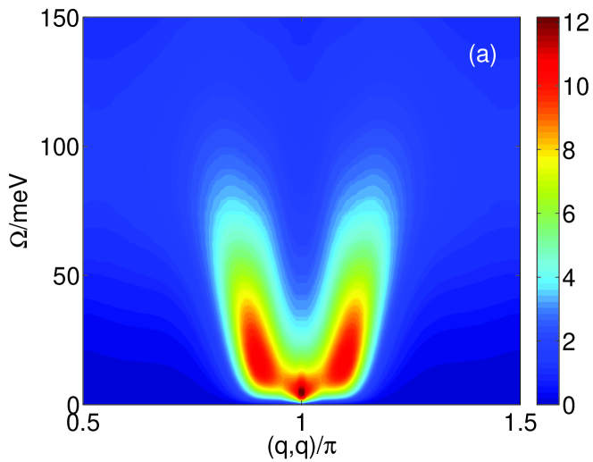
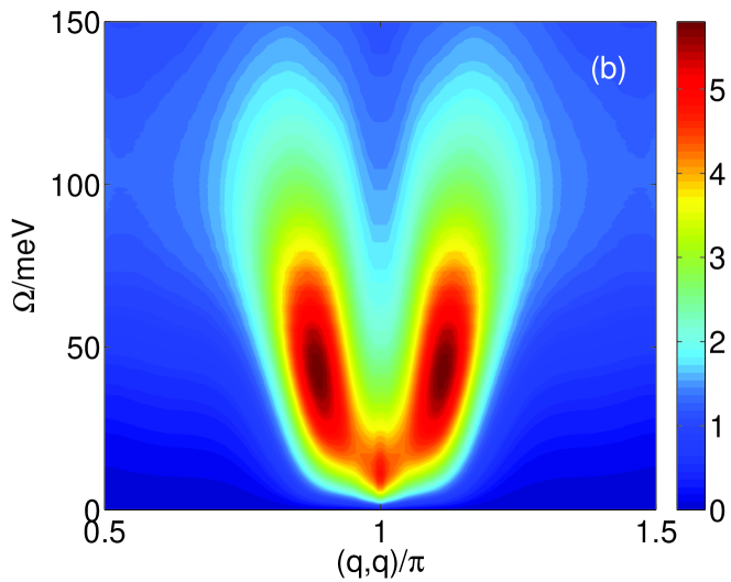
In Fig. 1, we show the imaginary part of for two different values of along the direction. For the larger value of (860 meV), Im is concentrated at low frequencies at the commensurate wavevector . This is typical of very underdoped samples near the commensurate antiferromagnetic phase Stock . We contrast this with a smaller value of (800 meV), where spectral weight is now concentrated at incommensurate wavevectors at a higher energy, being a more appropriate description of INS data Hinkov for slightly underdoped samples (consistent with the ARPES data set employed). Decreasing even further reduces the magnitude of Im , moves the incommensurate weight to even higher energies, and suppresses the lower energy commensurate weight.
Using this , the resulting electron-electron interaction is Monthoux ; Scalapino
| (4) |
where differs from because of vertex corrections Vilk . To set , we will require that the renormalized Fermi velocity at the d-wave node (the Fermi surface along the direction) matches that determined from the ARPES dispersion (1.6 eV) assuming a bare velocity of 3 eV from band theory. The renormalization factor (3/1.6) can be obtained as
| (5) |
where is the real part of the fermion self-energy, and we assume arises from the same interaction as above:
| (6) |
where is the bare fermion Green’s function
| (7) |
and is the bare dispersion (obtained from a tight binding fit to the ARPES dispersion by multiplying by the renormalization factor 3/1.6 mentioned above). The real part of is then obtained by analytic continuation. For the case shown in Fig. 1a, turns out to be the same as . But for the case shown in Fig. 1b, we must increase to 928 meV to obtain the same .
We now turn to the pairing problem. The anomalous (pairing) self-energy in the singlet channel is Monthoux ; Scalapino
| (8) |
with the pairing kernel
| (9) |
It is numerically convenient to solve this ‘linearized’ gap equation in the Matsubara representation (see Supplementary Information)
| (10) |
where is the bosonic (fermionic) Matsubara frequency, for a given bosonic (fermionic) function . In Eq. (9), is the fully dressed Green’s function, which is formally determined by including the self-energy correction Eq. (6) in a completely self-consistent approach. Instead, we obtain from the experimental spectral functions as discussed above using Eq. (10). This is related to the approach of Dahm et al Dahm where INS data were used instead.
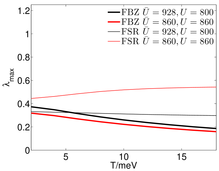
At Tc, the maximum eigenvalue () of Eq. (8) reaches unity and the corresponding eigenvector gives the energy-momentum structure of the superconducting order parameter. Ideally, we would need to know at each temperature. This is impractical when using real experimental data. Instead, we use our experimental normal state data at 140 K, and assume that all temperature dependence arises from the Matsubara frequencies. As we will see below, this is a best case scenario, since if anything, the magnitude of the pseudogap increases as the temperature is lowered.
Our results are shown in Fig. 2, labeled as FBZ (full Brillouin zone). We see that (which occurs for B1g, i.e., d-wave, symmetry) is much less than unity and essentially temperature independent for both cases shown in Fig. 1. This implies that there is no superconductivity. This is the central result of our paper.
To understand this surprising result, we now turn to Fermi surface restricted calculations, which is a commonly employed approximation where the momentum perpendicular to the Fermi surface () is integrated out. This approximation is equivalent to ignoring the dependence of on . This procedure results in an equation which depends only on the angular variation around the Fermi surface:
| (11) |
where is the number of angular points and is
| (12) |
is obtained by numerically integrating Eq. (9) using the experimental over , with the integration direction for each angle determined from the normal given by the tight binding fit to the ARPES data (this same procedure is used to identify in Eq. (1)).
The results are also shown in Fig. 2. Although is now temperature dependent, over the temperature range shown, it is still below unity. Paradoxically, increases with increasing temperature. We have verified that at even higher temperatures, reaches a maximum, and then begins to fall, with the more realistic second case (Fig. 1b) always remaining below unity. Similar behavior for the dependence of was reported by Maier et al Maier .
To understand this behavior, we now turn to some analytic calculations. To a good approximation, we can approximate for the d-wave case in the weak coupling BCS limit as
| (13) |
and assume an isotropic density of states over the Fermi surface coming from . The weak coupling equation for is
| (14) |
For we use a phenomenological form that is a good representation of ARPES data Norm07
| (15) |
Here is the broadening and the anisotropic pseudogap, which consistent with ARPES, is assumed to have a d-wave anisotropy. On the Fermi surface, this can be approximated as . The pairing kernel can now be analytically derived
| (16) |
Here is . To obtain an analytic approximation, we replace the sum by an integral , using the Euler-Maclaurin formula Abramowitz for low temperatures in Eq. (14) and rewrite the condition for Tc as
| (17) |
The integral over can be carried out analytically. The second term is convergent, so we can integrate it to . For the first term, we use a BCS cut-off energy and we assume and in the low limit we get
| (18) |
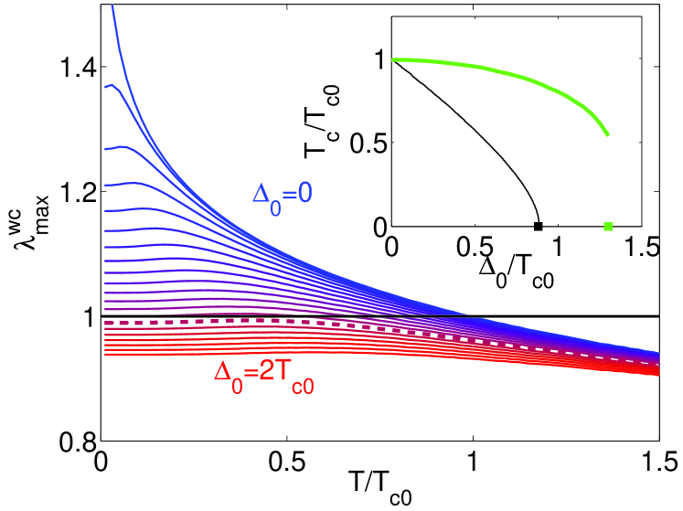
By examining Eq. (18), we can clearly see that the logarithmic divergence of the first term is cut-off by both and , so a solution is no longer guaranteed. We can estimate the critical values of the inverse lifetime and pseudogap to kill superconductivity at =0 for limiting cases. In the clean limit with , Tc0 where is Euler’s constant and Tc0 is Tc for . With no pseudogap, we find a critical inverse lifetime of (Abrikosov-Gor’kov AG ). Fig. 3 shows the numerically evaluated left hand side of Eq. (14) (denoted as ) as a function of temperature for various , with the variation of with or shown in the inset. One clearly sees the logarithmic divergence is cut-off as increases, leading to a maximum in at a particular temperature. Once this maximum falls below unity, no superconducting solution exists.
In order to show that our findings are general and not limited to weak coupling assumptions, we consider a calculation based on a derived from a phenomenological form for MMP ; Abanov :
| (19) |
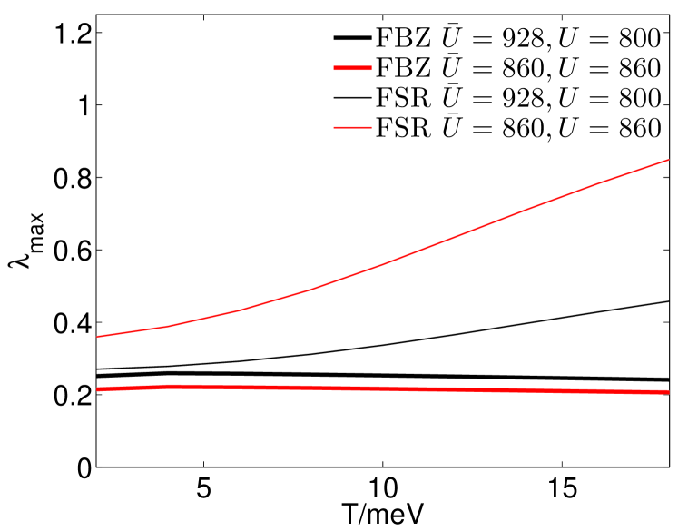
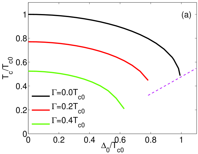
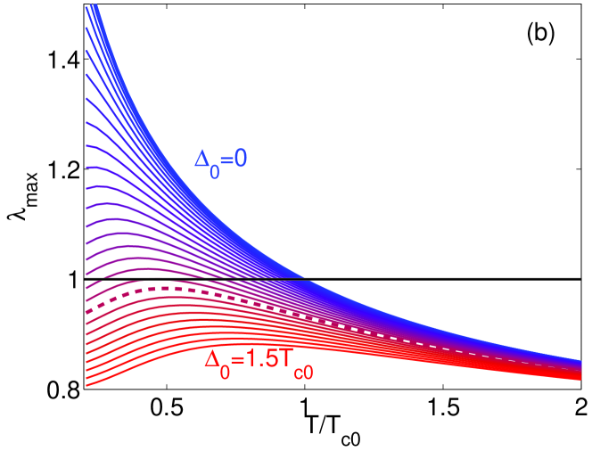
where is the coupling between fermions and spin fluctuations, is the antiferromagnetic coherence length, is the characteristic spin fluctuation energy scale, and is the static susceptibility at the commensurate vector . For illustrative purposes, we take eV, , eV with a cutoff energy for Im of 0.4 eV, though we have studied a variety of parameter sets (particularly variation of ). In general, these parameters are temperature dependent, but for simplicity we ignore this. We use the same model from above which was used to study the weak coupling limit. Fig. 4a shows the variation of with the pseudogap for different values of . As in the weak coupling case, and suppress Tc. As expected, the size of needed to destroy superconductivity is of order Tc0. The behavior of with temperature is similar to the weak coupling case, as illustrated in Fig. 4b. Again, a solution fails to appear once the temperature maximum of falls below unity. The same behavior was found in the Fermi surface restricted results presented in Fig. 1. In turn, use of our phenomenological and in the full Brillouin zone formalism leads to similar behavior to Fig. 1 as well, with weakly temperature dependent having values much less than unity (see Supplementary Information).
Over much of the doping-temperature phase diagram of the cuprates, ARPES reveals strongly lifetime broadened features with a large pseudogap above Tc. Despite this, Tc is large except under extreme underdoping conditions. The work presented above indicates that for such a large pseudogap, there should be no superconducting solution. In our phenomenological studies, this can be mitigated somewhat by using model Green’s functions Norm07 which have Fermi surfaces in the pseudogap phase (as occurs with charge ordering, spin ordering, or more phenomenological considerations like those of Yang, Rice and Zhang YRZ ). On the other hand, the fact that we find this same behavior using experimental Green’s functions indicates that this is a general issue, not specific to any particular model.
There is a way out of this dilemma. If the pseudogap were due to pairing, then all of the above conclusions are invalidated. In this case, the mean field Tc would actually be the temperature at which becomes non-zero, with the true Tc suppressed from this due to fluctuations. In a preformed pairs picture, Tc would be controlled by the phase stiffness of the pairs Emery , whereas in RVB theory, it would be controlled by the coherence temperature of the doped holes Wen . Regardless, our results are in strong support for such models. ARPES Amit ; Yang and tunneling (STM) Kohsaka ; Alldredge are consistent with a pairing pseudogap, since the observed spectra associated with the antinodal region of the zone have a minimum at zero bias as would be expected if the gap were due to pairing (local or otherwise). This does not mean that charge and/or spin ordering does not occur in the pseudogap phase, it is just that our results are consistent with these phenomena not being responsible for the pseudogap itself.
References
- (1)
- (2)
References
Acknowledgments
The authors thank Doug Scalapino for suggesting this work, and he and Andrey Chubukov for several helpful discussions. This work was supported by the US DOE, Office of Science, under contract DE-AC02-06CH11357 and by the Center for Emergent Superconductivity, an Energy Frontier Research Center funded by the US DOE, Basic Energy Sciences, under Award No. DE-AC0298CH1088.
Supplementary material
.1 Pairing equations
For the full Brillouin zone calculations, we use a 64 by 64 point grid in the first Brillouin zone and a Matsubara cut-off of 40. For the Fermi surface restricted calculations, we use an angular step of 1 degree on the Fermi surface, with a Matsubara cut-off of 100. Convergence was tested for both the point sum and the Matsubara cut-off. The tight binding fit used for was that of Kaminski et al Adam05 .
Technically, we should be solving two coupled equations, one for and one for . But since we are equating to the experimental Green’s function from ARPES, we do not solve the equation. We note that the popular ‘trick’ of reducing these two equations to a single master equation in the Fermi surface restricted case does not work in the presence of a pseudogap. That is, the pseudogap can be represented in the functional form Norm07s
| (20) |
which can be easily generalized to include broadening. Here, is for the pairing case, and for density wave ordering at . The important point is because of the strong dependence of on , one cannot collapse to a simple master equation commonly used in Eliashberg calculations Abanov08 . We admit, though, that because we do not solve the equation (except to estimate ), we could be overestimating pair breaking effects.
.2 Temperature dependent models
To mimic the temperature dependence of the spectral function, we can allow and to be dependent in
| (21) |
Based on the ARPES data, we take to be temperature independent. For the Fermi surface restricted calculations, it has the form with a of 50 meV. For the full Brillouin zone calculations, it has the form with a of 54 meV. In both cases, we again use constructed from the experimental Green’s functions, and so the in Eq. (21) is just used in the part of the pair vertex. With a temperature independent =50 meV, we find similar behavior in the pairing equation as when we use the experimental spectral functions. Next we consider a more realistic model where behaves linearly with as in marginal Fermi liquid theory (here, we use a coefficient in front of T of 5.58 to reproduce the pseudogap temperature T∗ of 180 K for this sample, since this form for will becomes gapless at the anti-node Norm07s once ). Again, the behavior of with T is similar to before, as shown in Fig. 5.
References
- (1)
- (2)
References