Cooperative Set Aggregation for Multiple Lagrangian Systems

Abstract

In this paper, we study the cooperative set tracking problem for a group of Lagrangian systems. Each system observes a convex set as its local target. The intersection of these local sets is the group aggregation target. We first propose a control law based on each system’s own target sensing and information exchange with neighbors. With necessary connectivity for both cases of fixed and switching communication graphs, multiple Lagrangian systems are shown to achieve rendezvous on the intersection of all the local target sets while the vectors of generalized coordinate derivatives are driven to zero. Then, we introduce the collision avoidance control term into set aggregation control to ensure group dispersion. By defining an ultimate bound on the final generalized coordinate between each system and the intersection of all the local target sets, we show that multiple Lagrangian systems approach a bounded region near the intersection of all the local target sets while the collision avoidance is guaranteed during the movement. In addition, the vectors of generalized coordinate derivatives of all the mechanical systems are shown to be driven to zero. Simulation results are given to validate the theoretical results.

I Introduction

Along with the rapid development of coordination of multi-agent systems (see e.g., [1, 2, 3, 4, 5, 6, 7, 8]), the study on the distributed control of multiple Lagrangian systems has attracted extensive attention during the last decade. Compared with the single integrator dynamics, a Lagrangian model can be used to describe mechanical systems, such as mobile robots, autonomous vehicles, robotic manipulators, and rigid bodies. Therefore, the study on the distributed control of multiple Lagrangian systems is more applicable to the applications including spacecraft formation flying and relative attitude keeping and control of multiple unmanned aerial vehicles, just named a few.

The key idea of distributed control is to realize a collective task for the overall system by using only neighboring information exchange [9, 10, 11, 12, 13, 14]. Such an algorithm relies on a setting that communication units are equipped for each individual system and thus a natural issue is communication link failure. Therefore, the analysis on the validness of distributed algorithm over a switching communication graph was investigated. Both continuous-time and discrete-time models were studied and many deep understanding was obtained for linear models [9, 15, 16]. Nonlinear multi-agent dynamics has also drawn much attention [17, 18] since in many practical problems the node dynamics is naturally nonlinear, e.g., Vicsek’s model and the Kuramoto’s model [1, 19].

For the coordination problem of multiple Lagrangian systems, the author of [20] proposed distributed model-independent consensus algorithms for multiple Lagrangian systems in a leaderless setting. The case of time-varying leader was studied in [21], where the nonlinear contraction analysis was introduced to obtain globally exponential convergence results. The connectedness maintenance problem was studied for multiple nonholonomic robotics in [22] and finite-time cooperative tracking algorithms were presented in [23] over graphs that are quasi-strongly connected. Distributed containment control was proposed in [24] and a sliding mode based strategy was introduced to estimate the leaders’ generalized coordinate derivative information. A similar problem was also studied in [25], where continuous control algorithms were proposed to guarantee cooperative tracking with bounded errors. The authors of [26] established containment, group dispersion and group cohesion behaviors for multiple Lagrangian systems, where both the cases of constant and time-varying leaders’ velocities were considered. In addition, the applications of the coordination algorithms on shape control and robotic manipulator synchronization were given, respectively, in [27] and [28].

In this work, we focus on the cooperative set tracking problem of multiple Lagrangian systems. The set target is used to describe a common region for all the systems and each system has access to only the constrained information on this common set target. We first propose a control guaranteeing the set aggregation for all the systems over fixed graphs. Then we extend the result to the case of switching graphs and that of the collision avoidance requirements. The main contributions of our results are as follows:

• A cooperative set tracking control is proposed for multiple Lagrangian systems. It is shown that under a general connectivity assumption for both fixed and switching graphs, multiple Lagrangian systems achieve rendezvous on the intersection of all the local target sets while the vectors of generalized coordinate derivatives are driven to zero.

• Collision avoidance is guaranteed during the movement. In addition, we show that multiple Lagrangian systems approach a bounded region near the intersection of all the local target sets while the vectors of generalized coordinate derivatives are driven to zero.

The remainder of the paper is organized as follows. In Section II, we give some basic notations and definitions on convex analysis, graph theory, Dini derivatives, and state the problem definition. A result for fixed interaction graphs is given in Section III. Then the cases with switching graphs and collision avoidance requirements are discussed in Sections IV and V. A brief concluding remark is given in Section VI.

II Preliminaries

In this section, we introduce some mathematical preliminaries on convex analysis [29], graph theory [30], and Dini derivatives [31]. We also state the problem definition of this paper.

II-A Convex analysis

Denote $\|\cdot\|$ the Euclidean norm. For any nonempty set $\mathcal{S}\subseteq\mathbb{R}^{m}$, we use $\|x\|_{\mathcal{S}}=\inf_{y\in\mathcal{S}}\|x-y\|$ to describe the distance between $x\in\mathbb{R}^{m}$ and $\mathcal{S}$. A set $\mathcal{S}\subset\mathbb{R}^{m}$ is called convex if $(1-\zeta)x+\zeta y\in\mathcal{S}$ when $x\in\mathcal{S}$, $y\in\mathcal{S}$, and $0\leq\zeta\leq 1$.

Let $\mathcal{S}$ be a convex set. The convex projection of any $x\in\mathbb{R}^{m}$ onto $\mathcal{S}$ is denoted by $P_{\mathcal{S}}(x)\in\mathcal{S}$ satisfying $\|x-P_{\mathcal{S}}(x)\|=\|x\|_{\mathcal{S}}$. We also know that $\|x\|_{\mathcal{S}}^{2}$ is continuously differentiable for all $x\in\mathbb{R}^{m}$, and its gradient can be explicitly obtained by [29]:

$$\nabla\|x\|_{\mathcal{S}}^{2}=2(x-P_{\mathcal{S}}(x)).$$ (1)

Also, it is trivial to see that

$$(P_{\mathcal{S}}(x)-x)^{\rm\tiny T}(P_{\mathcal{S}}(x)-y)\leq 0,~{}~{}\forall y\in\mathcal{S}.$$ (2)

II-B Graph theory

An undirected graph $\mathcal{G}$ consists of a pair $(\mathcal{V},\mathcal{E})$, where $\mathcal{V}=\{1,2,\ldots,n\}$ is a finite, nonempty set of nodes and $\mathcal{E}\subseteq\mathcal{V}\times\mathcal{V}$ is a set of unordered pairs of nodes. An arc $\{j,i\}\in\mathcal{E}$ denotes that node $i,j$ can obtain each other’ information mutually. All neighbors of node $i$ are denoted $\mathcal{N}_{i}:=\{j:\{j,i\}\in\mathcal{E}\}$. A path is a sequence of arcs of the form $\{i_{1},i_{2}\},\{i_{2},i_{3}\},\dots$. An undirected graph $\mathcal{G}$ is said to be connected if each node has an undirected path to any other node.

The adjacency matrix $A=[a_{ij}]\in\mathbb{R}^{n\times n}$ associated with the graph $\mathcal{G}$ is defined such that $a_{ij}$ is positive if $\{j,i\}\in\mathcal{E}$ and $a_{ij}=0$ otherwise. We also assume that $a_{ij}=a_{ji}$, for all $i,j\in\mathcal{V}$ for the undirected graph in this paper. The Laplacian matrix $L=[l_{ij}]\in\mathbb{R}^{n\times n}$ associated with $A$ is defined as $l_{ii}=\sum_{j\neq i}a_{ij}$ and $l_{ij}=-a_{ij}$, where $i\neq j$.

II-C Dini derivatives

Let $D^{+}V(t,x(t))$ be the upper Dini derivative of $V(t,x(t))$ with respect to $t$, i.e.,

$$D^{+}V(t,x)=\lim_{\tau\rightarrow 0^{+}}\sup\frac{V(t+\tau,x(t+\tau))-V(t,x(t))}{\tau}.$$

The following lemma is useful [32].

Lemma 1

Suppose for each $i\in\mathcal{V}$, $V_{i}:\mathbb{R}\times\mathbb{R}^{m}\rightarrow\mathbb{R}$ is continuously differentiable. Let $V(t,x)=\max_{i\in\mathcal{V}}V_{i}(t,x)$, and let $\mathcal{V}_{1}(t)=\{i\in\mathcal{V}:V_{i}(t,x(t))=V(t,x(t))\}$ be the set of indices where the maximum is reached at time $t$. Then

$$D^{+}V(t,x(t))=\max_{i\in\mathcal{V}_{1}(t)}\dot{V}_{i}(t,x(t)).$$

II-D Problem Definition

Consider a network with $n$ agents labeled by $\mathcal{V}=\{1,2,\ldots,n\}$. The dynamics of agent $i$ is described by the Lagrangian equations

$$M_{i}(q_{i})\ddot{q}_{i}+C_{i}(q_{i},\dot{q}_{i})\dot{q}_{i}=\tau_{i},~{}i=1,2,\dots,n,$$ (3)

where $q_{i}\in\mathbb{R}^{m}$ is the vector of generalized coordinates, $M_{i}(q_{i})\in\mathbb{R}^{m\times m}$ is the $m\times m$ inertia (symmetric) matrix, $C_{i}(q_{i},\dot{q}_{i})\dot{q}_{i}$ is the Coriolis and centrifugal terms, and $\tau_{i}\in\mathbb{R}^{m}$ is the control force. The dynamics of a Lagrangian system satisfies the following properties [33]:

1. $M_{i}(q_{i})$ is positive definite and is bounded for any $q_{i}\in\mathbb{R}^{m}$.

2. $\dot{M}_{i}(q_{i})-2C_{i}(q_{i},\dot{q}_{i})$ is skew symmetric.

3. $C_{i}(q_{i},\dot{q}_{i})$ is bounded with respect to $q_{i}$ and linearly bounded with respect to $\dot{q}_{i}$. More specifically, there is positive constant $k_{C}$ such that $\|C_{i}(q_{i},\dot{q}_{i})\|\leq k_{C}\|\dot{q}_{i}\|$.

The objective of the group is to drive the multi-agent systems converge to a common region. Different from the existing works, we consider a set target objective instead of a point target objective. The exact information of this common region is not available for all the agents. Instead, the constrained information for the region can be obtained by each agent using its’ own sensor. We use set $\mathcal{X}_{i}$, $i\in\mathcal{V}$, to denote this available information for agent $i$. The global objective is to design a set aggregation control such that all the agents converge to the intersection of all $\mathcal{X}_{i}$, $i\in\mathcal{V}$, i.e., $\mathcal{X}_{0}=\bigcap_{i}\mathcal{X}_{i}$. At each time, each agent observes the boundary points of its local available set and obtain the relative distance information between the local available set and itself. Also, the state information of each agent are exchanged by equipping each agent with simple and cheap communication unit. The sketch map of the cooperative set tracking problem is presented in Fig. 1.

Based on these information, we first construct a set aggregation control for fixed graphs and switching graphs. Then, we consider set aggregation problem with collision avoidance control, where the relative distance information between different agents are used to derive a collision avoidance control. In the following, we impose a standing assumption on set $\mathcal{X}_{i}$, $i\in\mathcal{V}$.

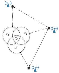
Figure 1: Cooperative set tracking problem

Assumption 1. $\mathcal{X}_{1},\mathcal{X}_{2},\dots,\mathcal{X}_{n}$ are closed convex sets, and $\mathcal{X}_{0}=\bigcap_{i=1}^{n}\mathcal{X}_{i}$ is nonempty and bounded.

We introduce the following definition on cooperative set aggregation.

Definition 1

Multi-agent system (3) achieves cooperative set aggregation if

1. $\lim_{t\rightarrow\infty}\|q_{i}(t)\|_{\mathcal{X}_{0}}=0,\quad\forall i\in\mathcal{V}$,

2. $\lim_{t\rightarrow\infty}(q_{i}(t)-q_{j}(t))=0,\quad\forall i,j\in\mathcal{V}$,

3. $\lim_{t\rightarrow\infty}\dot{q}_{i}(t)=0,\quad\forall i\in\mathcal{V}$.

Remark 1

In fact, this set aggregation problem under convexity assumptions was a classical problem in optimization, where projected consensus algorithm was a standard solution [34]. This algorithm was then generalized to distributed versions via consensus dynamics in [35, 36]. However, all these existing algorithms are designed for agents with first-order dynamics, and are therefore not applicable to the problem studied in this paper.

In order to solve this problem, we construct the following algorithm

$$\tau_{i}=\tau^{non}_{i}+\tau^{v}_{i}+\tau^{s}_{i}+\tau^{in}_{i}+\tau^{a}_{i},$$ (4)

where $\tau^{non}_{i}$ represents nonlinear damping, $\tau^{v}_{i}$ represents generalized coordinate derivative damping, $\tau^{s}_{i}$ represents self-target tracking, $\tau^{in}_{i}$ represents inter coordination of different systems, and $\tau^{a}_{i}$ represents the collision avoidance control. We next specify the designs of different control terms in different cases.

III Cooperative aggregation over fixed communication graphs

Let an undirected graph $\mathcal{G}=(\mathcal{V},\mathcal{E})$ define the communication graph. Moreover, recall that $j$ is a neighbor of $i$ when $\{j,i\}\in\mathcal{E}$, and $\mathcal{N}_{i}$ represents the set of agent $i$’s neighbors. The following control law is proposed for all $i\in\mathcal{V}$:

$$\tau_{i}=\underbrace{-k\dot{q}_{i}}_{\tau^{v}_{i}}\underbrace{-(q_{i}-P_{\mathcal{X}_{i}}(q_{i}))}_{\tau^{s}_{i}}\underbrace{-\sum_{j\in\mathcal{N}_{i}}a_{ij}(q_{i}-q_{j})}_{\tau^{in}_{i}},$$ (5)

where $k>0$ denotes generalized coordinate derivative damping, $a_{ij}>0$ for all $i,j$ marks the strength of the information flow between $i$ and $j$.

Theorem 1

Suppose that Assumption 1 hold. The multi-agent system (3) with (5) achieves set aggregation in the sense of Definition 1 if the fixed communication graph $\mathcal{G}$ is connected.

• Consider the following Lyapunov function:

  $$V= ~{}\frac{1}{2}\sum_{i=1}^{n}\dot{q}_{i}^{\rm\tiny T}M_{i}(q_{i})\dot{q}_{i}+\frac{1}{4}\sum_{i=1}^{n}\sum_{j\in\mathcal{N}_{i}}a_{ij}\|q_{i}-q_{j}\|^{2}$$

  $$+\frac{1}{2}\sum_{i=1}^{n}\|q_{i}-P_{\mathcal{X}_{i}}(q_{i})\|^{2}.$$

  The derivative of $V$ along (3) with (5) is

  $$\dot{V}= ~{}\sum_{i=1}^{n}\dot{q}_{i}^{\rm\tiny T}\left(\frac{1}{2}\dot{M}_{i}(q_{i})\dot{q}_{i}+M_{i}(q_{i})\ddot{q}_{i}\right)$$

  $$\!+\!\frac{1}{2}\sum_{i=1}^{n}\sum_{j\in\mathcal{N}_{i}}a_{ij}(q_{i}-q_{j})^{\rm\tiny T}(\dot{q}_{i}-\dot{q}_{j})\!+\!\!\sum_{i=1}^{n}\dot{q}_{i}^{\rm\tiny T}(q_{i}-P_{\mathcal{X}_{i}}(q_{i}))$$

  $$= ~{}\sum_{i=1}^{n}\dot{q}_{i}^{\rm\tiny T}\left(-k\dot{q}_{i}-\sum_{j\in\mathcal{N}_{i}}a_{ij}(q_{i}-q_{j})-(q_{i}-P_{\mathcal{X}_{i}}(q_{i}))\right)$$

  $$+\sum_{i=1}^{n}\dot{q}_{i}^{\rm\tiny T}\sum_{j\in\mathcal{N}_{i}}a_{ij}(q_{i}-q_{j})+\sum_{i=1}^{n}\dot{q}_{i}^{\rm\tiny T}(q_{i}-P_{\mathcal{X}_{i}}(q_{i}))$$

  $$= ~{}-k\sum_{i=1}^{n}\|\dot{q}_{i}\|^{2}$$

  $$\leq ~{}0,$$

  where we have used (1) to derive the first equality and the fact that $a_{ij}=a_{ji}$ and the second property of Lagrangian dynamics to derive the second equality.

  Therefore, based on LaSalle’s Invariance Principle (Theorem 4.4 of [37]), we know that every solution of (3) with (5) converges to largest invariant set in $\mathcal{M}$, where $\mathcal{M}=\{q_{i}\in\mathbb{R}^{m},\dot{q}_{i}\in\mathbb{R}^{m},~{}\forall i\in\mathcal{V}~{}|~{}\dot{q}_{i}=0,\forall i\in\mathcal{V}\}$. Let $q_{i}(t)$, $\dot{q}_{i}(t)$, $\forall i\in\mathcal{V}$ be a solution that belongs to $\mathcal{M}$:

  $$\dot{q}_{i}\equiv 0,~{}~{}\forall i\in\mathcal{V}\Rightarrow\ddot{q}_{i}\equiv 0,~{}~{}\forall i\in\mathcal{V}.$$

  It then follows from (3) and (5) that for all $i\in\mathcal{V}$,

  $$\tau_{i}\equiv 0\Rightarrow\sum_{j\in\mathcal{N}_{i}}a_{ij}(q_{i}-q_{j})+(q_{i}-P_{\mathcal{X}_{i}}(q_{i}))\equiv 0.$$

  Pick any $q_{0}\in\mathcal{X}_{0}$. Such a $q_{0}$ exists due to Assumption 1. Thus, it follows that for all $i\in\mathcal{V}$,

  $$(q_{i}-q_{0})^{\rm\tiny T}\sum_{j\in\mathcal{N}_{i}}a_{ij}(q_{i}-q_{j})+(q_{i}-q_{0})^{\rm\tiny T} (q_{i}-P_{\mathcal{X}_{i}}(q_{i}))\equiv 0.$$

  We then know that

  $$\sum_{i=1}^{n}(q_{i}-q_{0})^{\rm\tiny T}\sum_{j\in\mathcal{N}_{i}}a_{ij}(q_{i}-q_{j})+\sum_{i=1}^{n}(q_{i}-q_{0})^{\rm\tiny T}(q_{i}-P_{\mathcal{X}_{i}}(q_{i}))\equiv 0.$$

  It follows that $\sum_{i=1}^{n}(q_{i}-q_{0})^{\rm\tiny T}\sum_{j\in\mathcal{N}_{i}}a_{ij}(q_{i}-q_{j})=\frac{1}{2}\sum_{i=1}^{n}\sum_{j\in\mathcal{N}_{i}}a_{ij}\|q_{i}-q_{j}\|^{2}\geq 0$ by noting that $a_{ij}=a_{ji}$. Also, we know from (2) that $(P_{\mathcal{X}_{i}}(q_{i})-q_{0})^{\rm\tiny T}(q_{i}-P_{\mathcal{X}_{i}}(q_{i}))\geq 0$. It then follows that

  $$(q_{i}-q_{0})^{\rm\tiny T}(q_{i}-P_{\mathcal{X}_{i}}(q_{i}))= ~{}\|q_{i}-P_{\mathcal{X}_{i}}(q_{i})\|^{2}$$

  $$+(P_{\mathcal{X}_{i}}(q_{i})-q_{0})^{\rm\tiny T}(q_{i}-P_{\mathcal{X}_{i}}(q_{i}))$$

  $$\geq ~{}\|q_{i}-P_{\mathcal{X}_{i}}(q_{i})\|^{2}$$

  $$\geq ~{}0.$$

  This shows that $\sum_{i=1}^{n}(q_{i}-q_{0})^{\rm\tiny T}\sum_{j\in\mathcal{N}_{i}}a_{ij}(q_{i}-q_{j})\equiv 0$, and $\|q_{i}-P_{\mathcal{X}_{i}}(q_{i})\|\equiv 0$, $\forall i\in\mathcal{V}$. Therefore, we know that $\lim_{t\rightarrow\infty}(q_{i}(t)-P_{\mathcal{X}_{i}}(q_{i}(t)))=0$, $\forall i\in\mathcal{V}$, and $\lim_{t\rightarrow\infty}(q_{i}(t)-q_{j}(t))=0$, $\forall i,j\in\mathcal{V}$. This shows that set aggregation is achieved in the sense of Definition 1.

In the following, we investigate the problem under switching communication graphs and collision avoidance, respectively, where the analysis becomes much more challenging.

IV Cooperative aggregation over switching communication graphs

One issue of introducing the communication unit is the possible communication link failure. The link failure becomes even more important when we consider the real applications including controlling multiple autonomous vehicles in the environments with limited power. Therefore, it is necessary to consider the case of switching communication graph. We associate the switching communication topology with a time-varying graph $\mathcal{G}_{\sigma(t)}=(\mathcal{V},\mathcal{E}_{\sigma(t)})$, where $\sigma:[t_{0},+\infty)\rightarrow\mathcal{P}$ is a piecewise constant function and $\mathcal{P}$ is finite set of all possible graphs. $\mathcal{G}_{\sigma(t)}$ remains constant for $t\in[t_{l},t_{l+1})$, $l=0,1,\dots$ and switches at $t=t_{l}$, $l=1,\dots$. In addition, we assume that $\inf_{l}(t_{l+1}-t_{l})\geq\tau_{d}>0$, $l=1,\dots$, where $\tau_{d}$ is a constant and this dwell time assumption is extensively used in the analysis of switched systems [38]. The joint graph of $\mathcal{G}_{\sigma(t)}$ during time interval $[t_{1},t_{2})$ is defined by $\mathcal{G}_{\sigma(t)}([t_{1},t_{2}))=\bigcup_{t\in[t_{1},t_{2})}\mathcal{G}(t)=(\mathcal{V},\bigcup_{t\in[t_{1},t_{2})}\mathcal{E}(t))$. Moreover, $j$ is a neighbor of $i$ at time $t$ when $\{j,i\}\in\mathcal{E}_{\sigma(t)}$, and $\mathcal{N}(\sigma(t))$ represents the set of agent $i$’s neighbors at time $t$.

Definition 2

$\mathcal{G}_{\sigma(t)}$ is uniformly jointly connected if there exists a constant $T>0$ such that $\mathcal{G}([t,t+T))$ is connected for any $t\geq t_{0}$.

The existence of the switching communication graph complexes the problem significantly. In order to simplify the problem, we assume that the exact information of system dynamical parameters are available and propose the following control

$$\tau_{i}= ~{}\underbrace{C_{i}(q_{i},\dot{q}_{i})\dot{q}_{i}}_{\tau_{i}^{non}}\underbrace{-kM_{i}(q_{i})\dot{q}_{i}}_{\tau_{i}^{v}}\underbrace{-M_{i}(q_{i})(q_{i}-P_{\mathcal{X}_{i}}(q_{i}))}_{\tau_{i}^{s}}$$

$$~{}\underbrace{-M_{i}(q_{i})\sum_{j\in\mathcal{N}_{i}(\sigma(t))}a_{ij}(t)(q_{i}-q_{j})}_{\tau_{i}^{in}},\qquad\forall i\in\mathcal{V},$$ (6)

where $k>0$ denotes generalized coordinate derivative damping, and continuous function $a_{ij}(t)>0$ is the weight of arc $\{j,i\}$ for $i,j\in\mathcal{V}$ at $t$. We also assume that $a_{ij}(t)$ satisfies the following condition:

Assumption 2. There exists constants $a^{*}>0$ and $a_{*}>0$ such that for all $i,j\in\mathcal{V}$,

$$a_{*}\leq a_{ij}(t)\leq a^{*},\quad t\in\mathbb{R}^{+}.$$

Closed-loop system of (3) and (6) is

$$\ddot{q}_{i}=-k\dot{q}_{i}-\sum_{j\in\mathcal{N}_{i}(\sigma(t))}a_{ij}(t)(q_{i}-q_{j})-(q_{i}-P_{\mathcal{X}_{i}}(q_{i})).$$ (7)

We next focus on the closed-loop system (7).

IV-A Local set aggregation

We first present a proposition regarding the local set aggregation of the closed-loop system (7). Based on this proposition, we then show global set aggregation.

Proposition 1

Suppose that Assumptions 1 and 2 hold and choose $k$ large enough. The states of the multi-agent system (3) with (6) achieve local target aggregation, i.e., $\lim_{t\rightarrow\infty}\|q_{i}(t)\|_{\mathcal{X}_{i}}=0$, and $\lim_{t\rightarrow\infty}\dot{q}_{i}(t)=0$, for all $i\in\mathcal{V}$.

• By picking any $q_{0}\in\mathcal{X}_{0}$, we propose the following Lyapunov function:

  $$V= ~{}\frac{1}{2}\sum_{i=1}^{n}\dot{q}_{i}^{\rm\tiny T}\dot{q}_{i}+\sum_{i=1}^{n}(q_{i}-q_{0})^{\rm\tiny T}\dot{q}_{i}+\frac{k}{2}\sum_{i=1}^{n}\|q_{i}-q_{0}\|^{2}$$

  $$+\frac{1}{2}\sum_{i=1}^{n}\|q_{i}-P_{\mathcal{X}_{i}}(q_{i})\|^{2},$$

  where we choose $k>1$ to guarantee $V$ is positive definite. The derivative of $V$ along (7) is

  $$\dot{V}= \sum_{i=1}^{n}\dot{q}_{i}^{\rm\tiny T}\left(\!\!-k\dot{q}_{i}-\!\!\!\!\!\!\sum_{j\in\mathcal{N}_{i}(\sigma(t))}a_{ij}(t)(q_{i}-q_{j})-(q_{i}-P_{\mathcal{X}_{i}}(q_{i}))\!\!\right)$$

  $$+\sum_{i=1}^{n}(q_{i}-q_{0})^{\rm\tiny T}\left(-k\dot{q}_{i}-\sum_{j\in\mathcal{N}_{i}(\sigma(t))}a_{ij}(t)(q_{i}-q_{j})\right.$$

  $$\left.-(q_{i}-P_{\mathcal{X}_{i}}(q_{i}))\!\!\frac{}{}\right)+\sum_{i=1}^{n}\|\dot{q}_{i}\|^{2}+k\sum_{i=1}^{n}(q_{i}-q_{0})^{\rm\tiny T}\dot{q}_{i}$$

  $$+\sum_{i=1}^{n}\dot{q}_{i}^{\rm\tiny T}(q_{i}-P_{\mathcal{X}_{i}}(q_{i}))$$

  $$= ~{}-(k-1)\sum_{i=1}^{n}\|\dot{q}_{i}\|^{2}-\sum_{i=1}^{n}\dot{q}_{i}^{\rm\tiny T}\sum_{j\in\mathcal{N}_{i}(\sigma(t))}a_{ij}(t)(q_{i}-q_{j})$$

  $$-\sum_{i=1}^{n}(q_{i}-q_{0})^{\rm\tiny T}(q_{i}-P_{\mathcal{X}_{i}}(q_{i}))-\sum_{i=1}^{n}(q_{i}-q_{0})^{\rm\tiny T}$$

  $$~{}\times\sum_{j\in\mathcal{N}_{i}(\sigma(t))}a_{ij}(t)(q_{i}-q_{j})$$

  $$\leq ~{}-\left[\begin{array}[]{cc}q(t)&\dot{q}(t)\end{array}\right]\left[\begin{array}[]{cc}L_{\sigma(t)}&\frac{L_{\sigma(t)}}{2}\\ \frac{L_{\sigma(t)}}{2}&(k-2)I_{n}\end{array}\right]\left[\begin{array}[]{c}q(t)\\ \dot{q}(t)\end{array}\right]$$

  $$-\sum_{i=1}^{n}\|q_{i}(t)\|_{\mathcal{X}_{i}}^{2}-\sum_{i=1}^{n}\|\dot{q}_{i}(t)\|^{2},$$

  where $q=[q_{1}^{\rm\tiny T},q_{2}^{\rm\tiny T},\dots,q_{n}^{\rm\tiny T}]^{\rm\tiny T}$, $q=[q_{1}^{\rm\tiny T},q_{2}^{\rm\tiny T},\dots,q_{n}^{\rm\tiny T}]^{\rm\tiny T}$, $L_{\sigma(t)}$ is Laplacian matrix associated with $\mathcal{G}_{\sigma(t)}$ at time $t$ defined in Section II-B, and we have used the fact that $(q_{i}-q_{0})^{\rm\tiny T}(q_{i}-P_{\mathcal{X}_{i}}(q_{i}))\geq\|q_{i}-P_{\mathcal{X}_{i}}(q_{i})\|^{2}$. It is trivial to show that $L_{p}$ is symmetric and positive semi-definite, for all $p\in\mathcal{P}$. Therefore, if $k$ is chosen such that $k>2+\frac{1}{4}\max_{p\in\mathcal{P}}\{\lambda_{\max}(L_{p})\}$, or equivalent, $k>2+\frac{(n-1)a^{*}}{2}$, we can show that $\left[\begin{array}[]{cc}L_{p}&\frac{L_{p}}{2}\\ \frac{L_{p}}{2}&(k-2)I_{n}\end{array}\right]$ is positive semi-definite, for all $p\in\mathcal{P}$. It then follows that

  $$\dot{V}\leq-\sum_{i=1}^{n}\|q_{i}\|_{\mathcal{X}_{i}}^{2}-\sum_{i=1}^{n}\|\dot{q}_{i}\|^{2}\leq 0.$$ (8)

  Therefore, $q_{i}$ and $\dot{q}_{i}$, $\forall i\in\mathcal{V}$ are bounded. We also know that (8) implies that

  $$\int_{t_{0}}^{\infty}\left(\sum_{i=1}^{n}\|q_{i}(t)\|_{\mathcal{X}_{i}}^{2}+\sum_{i=1}^{n}\|\dot{q}_{i}(t)\|^{2}\right){\rm d}t\leq V(t_{0})$$

  is bounded. In addition, it follows that $\frac{{\rm d}}{{\rm d}t}\left(\sum_{i=1}^{n}\|q_{i}(t)\|_{\mathcal{X}_{i}}^{2}+\sum_{i=1}^{n}\|\dot{q}_{i}(t)\|^{2}\right)\\ =~{}2\sum_{i=1}^{n}\left((q_{i}-P_{\mathcal{X}_{i}}(q_{i}))^{\rm\tiny T}\dot{q}_{i}+\dot{q}_{i}^{\rm\tiny T}\ddot{q}_{i}\right).$ Therefore, from (7) and the facts that $q_{i}$ and $\dot{q}_{i}$, $\forall i\in\mathcal{V}$ are bounded, we know that $\frac{{\rm d}}{{\rm d}t}\left(\sum_{i=1}^{n}\|q_{i}(t)\|_{\mathcal{X}_{i}}^{2}+\sum_{i=1}^{n}\|\dot{q}_{i}(t)\|^{2}\right)$ is bounded $\forall t\in\mathbb{R}^{+}$. Then, based on Barbalat’s lemma [37], we can show that $\sum_{i=1}^{n}\|q_{i}(t)\|_{\mathcal{X}_{i}}^{2}+\sum_{i=1}^{n}\|\dot{q}_{i}(t)\|^{2}\rightarrow 0$, as $t\rightarrow\infty$. Therefore, $\lim_{t\rightarrow\infty}\|q_{i}(t)\|_{\mathcal{X}_{i}}=0$, and $\lim_{t\rightarrow\infty}\dot{q}_{i}(t)=0$, for all $i\in\mathcal{V}$.

IV-B Global set aggregation

Next, we rewrite the closed-loop system (7) as

$$\dot{q}_{i}=\dot{q}_{i},$$ (9a)

$$\ddot{q}_{i}=-k\dot{q}_{i}-\sum_{j\in\mathcal{N}_{i}(\sigma(t))}a_{ij}(t)(q_{i}-q_{j})-(q_{i}-P_{\mathcal{X}_{i}}(q_{i})).$$ (9b)

Define $x_{i}=q_{i}$, $x_{n+i}=q_{i}+\frac{2}{k}\dot{q}_{i}$, for all $i\in\mathcal{V}$. After some manipulations, (9) can be written as

$$\dot{x}_{i}=-\frac{k}{2}(x_{i}-x_{n+i}),~{}~{}i=1,2,\dots,n$$ (10)

$$\dot{x}_{n+i}= -\frac{k}{2}(x_{n+i}-x_{i})-\frac{2}{k}\sum_{j\in\mathcal{N}_{i}(\sigma(t))}a_{ij}(t)(x_{n+i}-x_{n+j})$$

$$+\delta_{i}(t),~{}~{}i=1,2,\dots,n.$$

where $\delta_{i}=\frac{4}{k^{2}}\sum_{j\in\mathcal{N}_{i}(\sigma(t))}a_{ij}(t)(\dot{q}_{i}-\dot{q}_{j})-\frac{2}{k}(q_{i}-P_{\mathcal{X}_{i}}(q_{i}))$, for all $i\in\mathcal{V}$. Note that each entry of $x_{i}\in\mathbb{R}^{m}$ is decoupled, without loss of generality, we assume $m=1$ in the following analysis.

Define $\overline{\mathcal{V}}=\{1,2,\dots,2n\}$, and

$$\hbar(t)=\max_{i\in\overline{\mathcal{V}}}\{x_{i}(t)\},~{}~{}\ell(t)=\min_{i\in\overline{\mathcal{V}}}\{x_{i}(t)\}.$$

Lemma 2

For all $t\geq t_{0}\geq 0$, it follows that

$$D^{+}\hbar(t)\leq\max_{i\in\mathcal{V}}\|\delta_{i}\|,\quad D^{+}\ell(t)\geq-\max_{i\in\mathcal{V}}\|\delta_{i}\|.$$

Let $\overline{\mathcal{V}}_{1}(t)$ be the set containing all the agents that reach the maximum at time $t$, i.e., $\overline{\mathcal{V}}_{1}(t)=\{i\in\overline{\mathcal{V}}|x_{i}(t)=\hbar(t)\}$. It then follows from Lemma 1 that

$$D^{+}\hbar(t)\leq ~{}\max_{i\in\overline{\mathcal{V}}_{1}}\dot{x}_{i}(t)$$

$$\leq ~{}\max\left\{~{}\max_{i\in\overline{\mathcal{V}}_{1}\bigcap\{1,2,\dots,n\}}\frac{k}{2}(x_{n+i}-x_{i}),\right.$$

$$\max_{i\in\overline{\mathcal{V}}_{1}\bigcap\{n+1,n+2,\dots,2n\}}\frac{k}{2}(x_{i-n}-x_{i})$$

$$\left.\!\!+\frac{2}{k}\sum_{j\in\mathcal{N}_{i-n}(\sigma(t))}a_{(i-n)j}(t)(x_{n+j}-x_{i})+\delta_{i-n}(t)\!\!\right\}$$

$$\leq ~{}\max_{i\in\mathcal{V}(t)}\delta_{i}(t)$$

$$\leq ~{}\max_{i\in\mathcal{V}}\|\delta_{i}\|.$$

Similarly, we have that $D^{+}\ell(t)\geq-\max_{i\in\mathcal{V}}\|\delta_{i}\|$.

Theorem 2

Suppose that Assumptions 1 and 2 hold and choose $k$ large enough. The multi-agent system (3) with (6) achieves set aggregation in the sense of Definition 1 if the communication graph $\mathcal{G}_{\sigma(t)}$ is uniformly jointly connected.

• It follows from Proposition 1 that $\lim_{t\rightarrow\infty}\delta_{i}(t)=0$, for all $i\in\mathcal{V}$. This shows that for any $\varepsilon>0$, there exists $T_{1}(\varepsilon)>0$ such that

  $$\|\delta_{i}(t)\|\leq\varepsilon,\quad\forall i\in\mathcal{V},\quad t\geq T_{1}.$$

  It also follows from Proposition 1 that $x_{i}(t)$, for all $i\in\overline{\mathcal{V}}$, is bounded for all $t\geq t_{0}\geq 0$. Therefore, $\hbar(T_{1})$ and $\ell(T_{1})$ are bounded.

  The analysis of this theorem is motivated by [36]. Define $\overline{T}=T+2\tau_{d}$. We next focus on the time interval $t\in[T_{1},T_{1}+N\overline{T}]$, where $N=n+1$. It follows from Lemma 2 that

  $$\hbar(t)\leq\hbar(T_{1})+N\overline{T}\varepsilon,\quad\ell(t)\geq\ell(T_{1})-N\overline{T}\varepsilon.$$ (11)

  Without loss of generality, we assume that $\hbar(T_{1})\neq\ell(T_{1})$. Then, we consider a node $i_{0}\in\overline{\mathcal{V}}$, where we assume $i_{0}$ satisfies $x_{i_{0}}(T_{1})\leq\frac{1}{2}\hbar(T_{1})+\frac{1}{2}\ell(T_{1})=\hbar(T_{1})-\varepsilon_{0}$, and $\varepsilon_{0}=\frac{1}{2}(\hbar(T_{1})-\ell(T_{1}))>0$. We first assume that $i_{0}\in\mathcal{V}$. It follows from (11) that for all $t\in[T_{1},T_{1}+N\overline{T}]$,

  $$\dot{x}_{i_{0}}(t)\leq-\frac{k}{2} \left(x_{i_{0}}(t)-\hbar(T_{1})-N\overline{T}\varepsilon\right).$$

  By using Gronwall’s inequality, we know that for all $t\in[T_{1},T_{1}+N\overline{T}]$,

  $$x_{i_{0}}(t)\leq ~{}x_{i_{0}}(T_{1})e^{-\frac{k}{2}(t-T_{1})}+(1-e^{-\frac{k}{2}(t-T_{1})})(\hbar(T_{1})+N\overline{T}\varepsilon)$$

  $$\leq ~{}\hbar(T_{1})-e^{-\frac{k}{2}(t-T_{1})}\varepsilon_{0}+N\overline{T}\varepsilon$$

  $$\leq ~{}\hbar(T_{1})-\overline{\varepsilon}_{0}+N\overline{T}\varepsilon,$$ (12)

  where $\overline{\varepsilon}_{0}=e^{-kN\overline{T}/2}\varepsilon_{0}$. It then follows that for all $t\in[T_{1},T_{1}+N\overline{T}]$,

  $$\dot{x}_{i_{0}+n}(t)\leq ~{}-\frac{k}{2}(x_{i_{0}+n}(t)-x_{i_{0}}(t))-\frac{2}{k}\left(\sum_{j=1}^{n}a_{i_{0}j}(t)\right)$$

  $$~{}\times(x_{i_{0}+n}(t)-\hbar(T_{1})-N\overline{T}\varepsilon)+\varepsilon$$

  It then follows from (12) that

  $$\dot{x}_{i_{0}+n}(t)\leq ~{}-\frac{k}{2}(x_{i_{0}+n}(t)-(\hbar(T_{1})-\overline{\varepsilon}_{0}+N\overline{T}\varepsilon))$$

  $$~{}-\alpha(x_{i_{0}+n}(t)-\hbar(T_{1})-N\overline{T}\varepsilon)+\varepsilon$$

  $$\!\leq -\alpha_{1}(x_{i_{0}+n}(t)-(\hbar(T_{1})-\frac{k}{2\alpha_{1}}\overline{\varepsilon}_{0}+N\overline{T}\varepsilon))+\varepsilon,$$

  where $\alpha=\frac{2}{k}(n-1)a^{*}$ and $\alpha_{1}=\frac{k}{2}+\frac{2}{k}(n-1)a^{*}$. Thus, for all $t\in[T_{1},T_{1}+N\overline{T}]$,

  $$x_{i_{0}+n}(t)\leq ~{}\hbar(T_{1})-(1-e^{-\alpha_{1}(t-T_{1})})\frac{k}{2\alpha_{1}}\overline{\varepsilon}_{0}+(N\overline{T}+\frac{2}{k})\varepsilon$$

  Thus, we know that

  $$x_{i_{0}+n}(T_{1}+\overline{T})\leq ~{}\hbar(T_{1})-(1-e^{-\alpha_{1}\overline{T}})\frac{k}{2\alpha_{1}}\overline{\varepsilon}_{0}$$

  $$+(N\overline{T}+\frac{2}{k})\varepsilon$$

  Therefore, for all $t\in[T_{1}+\overline{T},T_{1}+N\overline{T}]$, it follows that

  $$x_{i_{0}+n}(t)\leq ~{}\hbar(T_{1})-(1-e^{-\alpha_{1}\overline{T}})\frac{k}{2\alpha_{1}}e^{-\alpha_{1}N\overline{T}}\overline{\varepsilon}_{0}$$

  $$+(N\overline{T}+\frac{4}{k})\varepsilon$$

  Instead, if $i_{0}\in\{n+1,n+2,\dots,2n\}$, it follows from (11) that for all $t\in[T_{1},T_{1}+N\overline{T}]$,

  $$\dot{x}_{i_{0}}(t)\leq-\alpha_{1}\left(x_{i_{0}}(t)-\hbar(T_{1})-N\overline{T}\varepsilon\right)+\varepsilon.$$

  By using Gronwall’s inequality, we know that for all $t\in[T_{1},T_{1}+N\overline{T}]$,

  $$x_{i_{0}}(t)\leq~{}\hbar(T_{1})-e^{-\alpha_{1}N\overline{T}}\varepsilon_{0}+(N\overline{T}+\frac{2}{k})\varepsilon,$$

  Therefore, we know that there exists a $i_{0}\in\mathcal{V}$ satisfying

  $$x_{i_{0}+n}(t)\leq~{}\hbar(T_{1})-\overline{\varepsilon}_{1}+(N\overline{T}+\frac{4}{k})\varepsilon$$

  for all $t\in[T_{1}+\overline{T},T_{1}+N\overline{T}]$, where $\overline{\varepsilon}_{1}=(1-e^{-\alpha_{1}\overline{T}})\frac{k}{2\alpha_{1}}e^{-\alpha_{1}N\overline{T}}e^{-\frac{k}{2}N\overline{T}}\varepsilon_{0}$.

  Next, based on the fact that $\mathcal{G}_{\sigma(t)}$ is uniformly jointly connected, we know that $i_{0}+n$ is jointly connected to other node $j\in\{n+1,n+2,\dots,2n\}/(i_{0}+n)$ during the time interval $[T_{1}+\overline{T},T_{1}+\overline{T}+T]$. Therefore, there exists $[T_{2},T_{2}+\tau_{d}]\subset[T_{1}+\overline{T},T_{1}+2\overline{T}]$ such that there is a $j\in\{n+1,n+2,\dots,2n\}/(i_{0}+n)$ being the neighbor of $i_{0}+n$ during $[T_{2},T_{2}+\tau_{d}]$. Denote this node as $i_{1}+n$. We next establish an upper bound for $x_{i_{1}+n}(t)$. For any $t\in[T_{2},T_{2}+\tau_{d}]$, we consider two cases:

  Case I: $x_{i_{1}+n}(t)>x_{i_{0}+n}(t)$ for all $t\in[T_{2},T_{2}+\tau_{d}]$. It then follows that

  $$\dot{x}_{i_{1}+n}(t)\leq ~{}-\left(\frac{k}{2}+\frac{2}{k}a^{*}(n-2)\right)\left(x_{i_{1}+n}-\hbar(T_{1})-N\overline{T}\varepsilon\right)$$

  $$~{}-\frac{2}{k}a_{i_{1}i_{0}}(t)\left(x_{i_{1}+n}(t)-x_{i_{0}+n}(t)\right)+\varepsilon$$

  $$\leq ~{}-\left(\frac{k}{2}+\frac{2}{k}a^{*}(n-2)\right)\left(x_{i_{1}+n}-\hbar(T_{1})-N\overline{T}\varepsilon\right)$$

  $$~{}-\frac{2}{k}a_{*}\left(x_{i_{1}+n}-(\hbar(T_{1})-\overline{\varepsilon}_{1}+(N\overline{T}+\frac{4}{k})\varepsilon)\right)$$

  $$~{}+\varepsilon$$

  $$\leq ~{}-\alpha_{2}\left(x_{i_{1}+n}-\hbar(T_{1})+\frac{2a_{*}}{k\alpha_{2}}\overline{\varepsilon}_{1}-(2N\overline{T}+\frac{4}{k})\varepsilon\right)$$

  $$~{}+\varepsilon,$$

  where $\alpha_{2}=\frac{k}{2}+\frac{2}{k}a^{*}(n-2)+\frac{2}{k}a_{*}$ It then follows that

  $$x_{i_{1}+n}(T_{2}+\tau_{d})\leq ~{}\hbar(T_{1})-\left(1-e^{-\tau_{d}\alpha_{2}}\right)\frac{2a_{*}}{k\alpha_{2}}\overline{\varepsilon}_{1}$$

  $$~{}+(2N\overline{T}+\frac{6}{k})\varepsilon$$

  Therefore, it follows that for all $t\in[T_{2}+\tau_{d},T_{1}+N\overline{T}]$,

  $$x_{i_{1}+n}(t)\leq ~{}\hbar(T_{1})-e^{-N\overline{T}\alpha_{1}}\left(1-e^{-\tau_{d}\alpha_{2}}\right)\frac{2a_{*}}{k\alpha_{2}}\overline{\varepsilon}_{1}$$

  $$~{}+(2N\overline{T}+\frac{8}{k})\varepsilon.$$

  Case II: there exists a $t^{*}\in[T_{2},T_{2}+\tau_{d}]$ such that $x_{i_{1}+n}(t^{*})\leq x_{i_{0}+n}(t^{*})$. It thus follows that

  $$x_{i_{1}+n}(t^{*})\leq\hbar(T_{1})-\overline{\varepsilon}_{1}+(N\overline{T}+\frac{4}{k})\varepsilon.$$

  Therefore, we know that for all $t\in[t^{*},T_{1}+N\overline{T}]$,

  $$\dot{x}_{i_{1}+n}(t)\leq ~{}-\alpha_{1}\left(x_{i_{1}+n}(t)-\hbar(T_{1})-N\overline{T}\varepsilon\right)+\varepsilon.$$

  It then follows that

  $$x_{i_{1}+n}(t)\leq ~{}\hbar(T_{1})-e^{-N\overline{T}\alpha_{1}}\overline{\varepsilon}_{1}+(N\overline{T}+\frac{6}{k})\varepsilon.$$

  Combing Cases I and II, we know that for all $t\in[T_{2}+\tau_{d},T_{1}+N\overline{T}]$,

  $$x_{i_{1}+n}(t)\leq ~{}\hbar(T_{1})-\overline{\varepsilon}_{2}+(2N\overline{T}+\frac{8}{k})\varepsilon,$$

  where $\overline{\varepsilon}_{2}=e^{-N\overline{T}\alpha_{1}}\left(1-e^{-\tau_{d}\alpha_{2}}\right)\frac{2a_{*}}{k\alpha_{2}}\overline{\varepsilon}_{1}$.

  By repeating the above process during the time interval $[T_{1}+\gamma\overline{T},T_{1}+(\gamma+1)\overline{T}]$, $\gamma=2,3,\dots n-1$, we can show that for all $i\in\mathcal{V}$ and $t\in[T_{1}+n\overline{T},T_{1}+N\overline{T}]$,

  $$x_{i+n}(t)\leq~{}\hbar(T_{1})-\overline{\varepsilon}_{n}+(N\overline{T}+\frac{4}{k})n\varepsilon,$$

  where $\overline{\varepsilon}_{n}=e^{-N(n-1)\overline{T}\alpha_{1}}\left(1-e^{-\tau_{d}\alpha_{2}}\right)^{n-1}\left(\frac{2a_{*}}{k\alpha_{2}}\right)^{n-1}\overline{\varepsilon}_{1}$. Then, we know that for all $i\in\mathcal{V}$, and $t\in[T_{1}+n\overline{T},T_{1}+N\overline{T}]$,

  $$\dot{x}_{i}(t)\leq ~{}-\frac{k}{2}(x_{i}(t)-x_{i+n}(t))$$

  $$\leq ~{}-\frac{k}{2}(x_{i}(t)-(\hbar(T_{1})-\overline{\varepsilon}_{n}+(N\overline{T}+\frac{4}{k})n\varepsilon)).$$

  Therefore, it follows that for all $i\in\mathcal{V}$,

  $$\hbar(T_{1}+N\overline{T})\leq~{}\hbar(T_{1})-\overline{\varepsilon}_{n+1}+(N\overline{T}+\frac{4}{k})n\varepsilon,$$

  where $\overline{\varepsilon}_{n+1}=(1-e^{-\alpha_{1}N\overline{T}})\overline{\varepsilon}_{n}$.

  Otherwise, if $i_{0}$ satisfies $x_{i_{0}}(T_{1})\geq\frac{1}{2}\hbar(T_{1})+\frac{1}{2}\ell(T_{1})=\ell(T_{1})+\varepsilon_{0}$, we can similarly show that

  $$\ell(T_{1}+N\overline{T})\geq~{}\ell(T_{1})+\overline{\varepsilon}_{n+1}+(N\overline{T}+\frac{4}{k})n\varepsilon.$$

  It then follows that

  $$\hbar(T_{1}+N\overline{T})\!-\!\ell(T_{1}+N\overline{T})\!\leq ~{}\hbar(T_{1})\!-\!\ell(T_{1})-\overline{\varepsilon}_{n+1}$$

  $$~{}+(N\overline{T}+\frac{4}{k})n\varepsilon.$$

  This implies that

  $$\hbar(T_{1}+N\overline{T})\!-\!\ell(T_{1}+N\overline{T})\!\leq ~{}(1-\delta)(\hbar(T_{1})\!-\!\ell(T_{1}))$$

  $$~{}+(N\overline{T}+\frac{4}{k})n\varepsilon,$$

  where $\delta=e^{-N(n-1)\overline{T}\alpha_{1}}\left(1-e^{-\tau_{d}\alpha_{2}}\right)^{n-1}\left(\frac{2a_{*}}{k\alpha_{2}}\right)^{n-1}(1-e^{-\alpha_{1}\overline{T}})\frac{k}{4\alpha_{1}}e^{-(\alpha_{1}+\frac{k}{2})N\overline{T}}$. Then, for all $\xi=1,2,\dots,$, we obtain that

  $$\hbar(T_{1}+\xi N\overline{T})-\ell(T_{1}+\xi N\overline{T})\leq ~{}(1-\delta)^{\xi}(\hbar(T_{1})-\ell(T_{1}))$$

  $$~{}+\sum_{j=0}^{\xi-1}(1-\delta)^{j}(N\overline{T}+\frac{4}{k})n\varepsilon$$

  $$\leq ~{}(1-\delta)^{\xi}(\hbar(T_{1})-\ell(T_{1}))$$

  $$~{}+\frac{(N\overline{T}+\frac{4}{k})n\varepsilon}{\delta}.$$

  Thus,

  $$\lim_{\xi\rightarrow\infty}\sup(\hbar(T_{1}+\xi N\overline{T}) -\ell(T_{1}+\xi N\overline{T}))\leq\frac{(N\overline{T}+\frac{4}{k})n\varepsilon}{\delta},$$

  which shows that $\lim_{\xi\rightarrow\infty}\sup(\hbar(T_{1}+\xi N\overline{T})-\ell(T_{1}+\xi N\overline{T}))=0$ by choosing $\varepsilon$ sufficiently small. Therefore, we know that $\lim_{t\rightarrow\infty}(x_{i}(t)-x_{j}(t))=0$, for all $i,j\in\overline{\mathcal{V}}$. This implies that $\lim_{t\rightarrow\infty}(q_{i}(t)-q_{j}(t))=0$, for all $i,j\in\mathcal{V}$. This shows that set aggregation is achieved in sense of Definition 1.

IV-C Simulation Verifications

We now use numerical simulations to validate the effectiveness of the theoretical results obtained in Sections III and IV. We assume that there are eight agents ($n=8$) in the group. The system dynamics are given by [33],

$$\left[\begin{array}[]{cc}M_{11,i}&M_{12,i}\\ M_{21,i}&M_{22,i}\\ \end{array}\right]\left[\begin{array}[]{c}\ddot{q}_{ix}\\ \ddot{q}_{iy}\\ \end{array}\right]+ \left[\begin{array}[]{cc}C_{11,i}&C_{12,i}\\ C_{21,i}&C_{22,i}\\ \end{array}\right]\left[\begin{array}[]{c}\dot{q}_{ix}\\ \dot{q}_{iy}\\ \end{array}\right]$$

$$=\left[\begin{array}[]{c}\tau_{ix}\\ \tau_{iy}\\ \end{array}\right],i=1,2,\dots,8,$$

where $M_{11,i}=\theta_{1i}+2\theta_{2i}\cos q_{iy}$, $M_{12,i}=M_{21,i}=\theta_{3i}+\theta_{2i}\cos q_{iy}$, $M_{22,i}=\theta_{3i}$, $C_{11,i}=-\theta_{2i}\sin q_{iy}\dot{q}_{iy}$, $C_{12,i}=-\theta_{2i}\sin q_{iy}(\dot{q}_{ix}+\dot{q}_{iy})$, $C_{21,i}=\theta_{2i}\sin q_{iy}\dot{q}_{ix}$, $C_{22,i}=0$. We choose $\theta_{1i}=1.301$, $\theta_{2i}=0.256$, $\theta_{3i}=0.096$, $i=1,2,\dots,8$.

IV-C1 Fixed communication graphs

we assume that the available local sets of all the agents are circles, where the radius of the circles are $3$ and circles given by $\mathcal{X}_{1}=(1.5+3\cos(\theta),1.5+3\sin(\theta))$, $\mathcal{X}_{2}=(-1.5+3\cos(\theta),-1.5+3\sin(\theta))$, $\mathcal{X}_{3}=(1.5+3\cos(\theta),1.5+3\sin(\theta))$, and $\mathcal{X}_{4}=(3\cos(\theta),-1.5+3\sin(\theta))$, $\mathcal{X}_{5}=(3\cos(\theta),-1.5+3\sin(\theta))$, $\mathcal{X}_{6}=(-1.5+3\cos(\theta),-1.5+3\sin(\theta))$, $\mathcal{X}_{7}=(1+3\cos(\theta),1+3\sin(\theta))$, and $\mathcal{X}_{8}=(-1.5+3\cos(\theta),-1.5+3\sin(\theta))$ with $\theta\in[0,2\pi)$. The initial states of the agents are given by $q_{1}(0)=[-8,8]^{\rm\tiny T}$, $q_{2}(0)=[6.4,12]^{\rm\tiny T}$, $q_{3}(0)=[-8,-8]^{\rm\tiny T}$, $q_{4}(0)=[6,-8]^{\rm\tiny T}$, $q_{5}(0)=[-8.8,-4]^{\rm\tiny T}$, $q_{6}(0)=[4.8,-12]^{\rm\tiny T}$, $q_{7}(0)=[-4,-8]^{\rm\tiny T}$, $q_{8}(0)=[3.2,-12]^{\rm\tiny T}$, $\dot{q}_{1}(0)=[-0.4,0.4]^{\rm\tiny T}$, $\dot{q}_{2}(0)=[0.8,-0.8]^{\rm\tiny T}$, $\dot{q}_{3}(0)=[2.8,-2.8]^{\rm\tiny T}$, and $\dot{q}_{4}(0)=[1.6,-1.6]^{\rm\tiny T}$, $\dot{q}_{5}(0)=[-1.2,0.8]^{\rm\tiny T}$, $\dot{q}_{6}(0)=[1.6,-0.4]^{\rm\tiny T}$, $\dot{q}_{7}(0)=[1.6,-2]^{\rm\tiny T}$, and $\dot{q}_{8}(0)=[0.8,-0.8]^{\rm\tiny T}$. The control parameters are chosen by $k=1$. The communication graph $\mathcal{G}$ is given in Fig. 2. Also, the weight of adjacency matrix $A$ of the generalized coordinates associated with $\mathcal{G}$ is chosen to be $1$.

Figure 2: The communication graph $\mathcal{G}$ for Section IV-C1

Under the control (5), snapshots of generalized coordinates and trajectories of generalized coordinate derivatives of the agents are shown in Figs. 3, 4 and 5. We see that set aggregation is achieved.

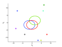
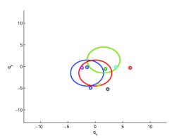
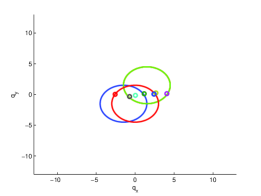
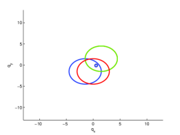
Figure 3: The trajectories of the generalized coordinates of the agents under control (5). The circles denote the generalized coordinates of the agents.

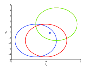
Figure 4: Zoom in of the final generalized coordinates of the agents under control (5).

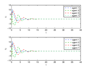
Figure 5: The trajectories of the generalized coordinate derivatives of the agents under control (5).

IV-C2 Switching communication graphs

we next consider the case of switching communication graphs. The system dynamics are given the same as those in Section IV-C1. The control parameter $k$ is chosen as $k=5$. The available local sets of all the agents are described by rectangles. The shapes of the rectangles are presented in Fig. 8 and the initial states of all agents are also the same as those given in Section IV-C1. The weight of adjacency matrix $A$ of the generalized coordinates associated with $\mathcal{G}$ is chosen to be $1$. The communication graph $\mathcal{G}$ switches between Fig. 6 and Fig. 7 at time instants $t_{\varrho}=5\varrho$, $\varrho=0,1,\dots$.

Figure 6: The communication graph $\mathcal{G}$ for Section IV-C2

Figure 7: The communication graph $\mathcal{G}$ for Section IV-C2

Under the control (6), snapshots of generalized coordinates and trajectories of generalized coordinate derivatives of the agents are shown in Figs. 8, 9 and 10. We see that set aggregation is achieved even when the communication graph is switching.

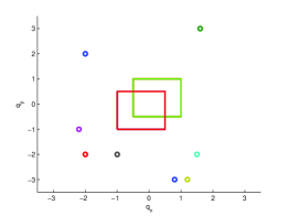
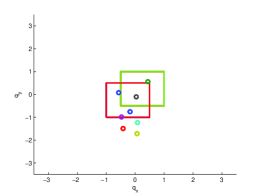
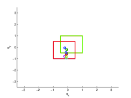
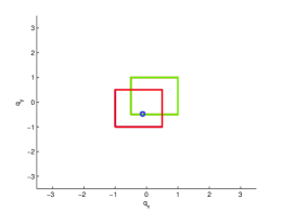
Figure 8: The trajectories of the generalized coordinates of the agents under control (6). The circles denote the generalized coordinates of the agents.

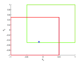
Figure 9: Zoom in of the final generalized coordinates of the agents under control (6).

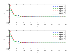
Figure 10: The trajectories of the generalized coordinate derivatives of the agents under control (6).

IV-C3 Discussions on the case of non-convex local sets

we next consider the case where $\mathcal{X}_{i}$, for all $i\in\mathcal{V}$ are non-convex sets. We assume that the available local sets of all the agents have irregular forms as shown in the Fig. 11. The initial states of the agents, the control parameter, the communication graph $\mathcal{G}$ are the same as those for Section IV-C1.

Under the control (5), snapshots of generalized coordinates and trajectories of generalized coordinate derivatives of the agents are shown in Figs. 11, 12 and 13. We see that set aggregation cannot be achieved. All the agents neither converge into their local sets nor reach a consensus. One way to overcome this side effect is to construct the convex hulls of all the local non-convex sets. By projecting the agents’ generalized coordinates onto the convex hulls of the local sets, we can still guarantee the set aggregation on the intersection of the convex hulls of the local sets using the proposed control. All these observations reveal the fundamental importance of the convexity of local sets in order for cooperative set aggregation.

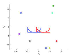
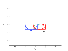
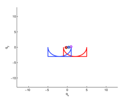
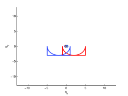
Figure 11: The trajectories of the generalized coordinates of the agents under control (5). The circles denote the generalized coordinates of the agents.

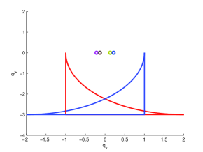
Figure 12: Zoom in of the final generalized coordinates of the agents under control (5)

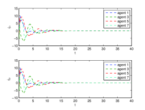
Figure 13: The trajectories of the generalized coordinate derivatives of the agents under control (5).

V Cooperative aggregation with collision avoidance

In certain practical applications, in addition to track a common objective using the constrained local information and information exchange, all the agents also need to guarantee collision avoidance during the movement. In such a case, global set aggregation cannot be achieved since there exist minimum safety distances between each pair of agents. Instead, multiple Lagrangian systems approach a bounded region near the intersection of all the local target sets while the collision avoidance is ensured during the movement. In this section, we investigate the considered cooperative set aggregation problem with collision avoidance also taken into consideration.

V-A Fixed Communication Graph: Approximate Aggregation

In this section, we assume that the communication graph is fixed. All the agents are also equipped with inter-agent sensors, where the sensing radius is denoted by $R$ and minimum safety radius is denoted by $r$ (see Fig. 14 for the illustration).

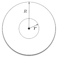
Figure 14: Sensing radius $R$ and minimum safety radius $r$

The following cooperative control with collision avoidance is proposed for all $i\in\mathcal{V}$,

$$\tau_{i}=\underbrace{-k\dot{q}_{i}}_{\tau_{i}^{v}}\underbrace{-(q_{i}-P_{\mathcal{X}_{i}}(q_{i}))}_{\tau_{i}^{s}}\underbrace{-\sum_{j\in\mathcal{N}_{i}}a_{ij}(q_{i}-q_{j})}_{\tau_{i}^{in}}\underbrace{-\sum_{j=1}^{n}\frac{\partial V_{ij}}{\partial q_{i}}}_{\tau_{i}^{a}},$$ (13)

where $k>0$ denotes generalized coordinate derivative damping, and motivated by [39], we define $V_{ij}=V_{ij}(\|q_{i}-q_{j}\|)$ as a positive function:

$$V_{ij}=\begin{cases}0,\quad~{}{\rm if}~{}\|q_{i}-q_{j}\|\geq R\\ \left(\frac{\|q_{i}-q_{j}\|-R^{2}}{\|q_{i}-q_{j}\|-r^{2}}\right)^{2},~{}~{}{\rm if}~{}~{}r<\|q_{i}-q_{j}\|<R,\end{cases}$$

where $R>r>0$ are positive constants. Then, we have that

$$\frac{\partial V_{ij}}{\partial q_{i}}=\begin{cases}0,\quad~{}\|q_{i}-q_{j}\|\geq R\\ \frac{4(R^{2}-r^{2})(\|q_{i}-q_{j}\|^{2}-R^{2})}{(\|q_{i}-q_{j}\|^{2}-r^{2})^{3}}(q_{i}-q_{j}),r<\|q_{i}-q_{j}\|<R.\end{cases}$$

Note that $V_{ij}$ is a differentiable, nonnegative function of the relative distance $\|q_{i}-q_{j}\|$ defined in $(r,\infty)$. Also note that $V_{ij}(\|q_{i}-q_{j}\|)\rightarrow\infty$ as $\|q_{i}-q_{j}\|\rightarrow r^{+}$.

Let $\mathcal{S}_{1},\mathcal{S}_{2},\dots,\mathcal{S}_{r}$ be closed convex sets with intersection $\mathcal{S}_{0}=\bigcap_{i=1}^{r}\mathcal{S}_{i}$ is nonempty. The collection $\{\mathcal{S}_{1},\mathcal{S}_{2},\dots,\mathcal{S}_{r}\}$ is said to be linearly regular [40] if there exists $\rho>0$ such that $\|x\|_{\mathcal{S}_{0}}\leq\rho\max_{i=1,2,\dots,r}\|x\|_{\mathcal{S}_{i}}$ for all $x\in\mathbb{R}^{m}$.

The main result we obtain is as follows, and it turns out certain approximate cooperative set aggregation can be achieved with collision avoidance guarantee.

Theorem 3

Let $\{\mathcal{X}_{1},\mathcal{X}_{2},\dots,\mathcal{X}_{n}\}$ be linearly regular and $\|q_{i}(t_{0})-q_{j}(t_{0})\|>r$, for all $i,j\in\mathcal{V}$. Suppose that Assumption 1 holds and the communication graph $\mathcal{G}$ is connected. Then the closed-loop system (3) with (13) ensures

1. $\|q_{i}(t)-q_{j}(t)\|>r,\quad\forall i,j\in\mathcal{V},\quad\forall t\geq t_{0}\geq 0$, where $r$ is a positive constant,

2. $\lim_{t\rightarrow\infty}\|q_{i}(t)\|_{\mathcal{X}_{0}}\leq B^{*},\quad\forall i\in\mathcal{V}$, where $B^{*}$ is a positive constant,

3. $\lim_{t\rightarrow\infty}\dot{q}_{i}(t)=0,\quad\forall i\in\mathcal{V}$.

• We propose the following Lyapunov function

  $$V= \frac{1}{2}\sum_{i=1}^{n}\dot{q}_{i}^{\rm\tiny T}M_{i}(q_{i})\dot{q}_{i}+\frac{1}{4}\sum_{i=1}^{n}\sum_{j\in\mathcal{N}_{i}}a_{ij}\|q_{i}-q_{j}\|^{2}$$

  $$+\frac{1}{2}\sum_{i=1}^{n}\|q_{i}-P_{\mathcal{X}_{i}}(q_{i})\|^{2}+\frac{1}{2}\sum_{i=1}^{n}\sum_{j=1}^{n}V_{ij}$$ (14)

  Note that the control term $\frac{\partial V_{ij}}{\partial q_{i}}$ does not introduce discontinuities because the potential function is differentiable at the transition point. The derivative of $V$ along (3) with (13) is

  $$\dot{V}= ~{}\sum_{i=1}^{n}\dot{q}_{i}^{\rm\tiny T}\left(-k\dot{q}_{i}-\sum_{j\in\mathcal{N}_{i}}a_{ij}(q_{i}-q_{j})-(q_{i}-P_{\mathcal{X}_{i}}(q_{i}))\right.$$

  $$\left.-\sum_{j=1}^{n}\frac{\partial V_{ij}}{\partial q_{i}}\right)+\frac{1}{2}\sum_{i=1}^{n}\sum_{j\in\mathcal{N}_{i}}a_{ij}(q_{i}-q_{j})^{\rm\tiny T}(\dot{q}_{i}-\dot{q}_{j})$$

  $$+\sum_{i=1}^{n}\dot{q}_{i}^{\rm\tiny T}(q_{i}-P_{\mathcal{X}_{i}}(q_{i}))+\frac{1}{2}\sum_{i=1}^{n}(\dot{q}_{i}-\dot{q}_{j})^{\rm\tiny T}\sum_{j=1}^{n}\frac{\partial V_{ij}}{\partial q_{i}}$$

  $$= ~{}-k\sum_{i=1}^{n}\dot{q}_{i}^{\rm\tiny T}\dot{q}_{i}-\sum_{i=1}^{n}\dot{q}_{i}^{\rm\tiny T}\sum_{j\in\mathcal{N}_{i}}a_{ij}(q_{i}-q_{j})$$

  $$+\sum_{i=1}^{n}\dot{q}_{i}^{\rm\tiny T}\sum_{j\in\mathcal{N}_{i}}a_{ij}(q_{i}-q_{j})$$

  $$= ~{}-k\sum_{i=1}^{n}\|\dot{q}_{i}\|^{2}$$

  $$\leq ~{}0,$$

  where we have used the fact $\frac{\partial V_{ij}}{\partial(q_{i}-q_{j})}=\frac{\partial V_{ij}}{\partial q_{i}}=-\frac{\partial V_{ij}}{\partial q_{j}}=\frac{\partial V_{ji}}{\partial q_{i}}=-\frac{\partial V_{ij}}{\partial q_{j}}$, for all $i,j\in\mathcal{V}$. Therefore, we know that $V(t)\leq V(t_{0})<\infty$ is bounded for all $t\geq t_{0}$. This further implies that $V_{ij}(t)\leq V(t_{0})$ is bounded for all $i,j\in\mathcal{V}$ and for all $t\geq t_{0}$. This shows that the collision avoidance is guaranteed, i.e., $\|q_{i}(t)-q_{j}(t)\|>r,~{}\forall i,j\in\mathcal{V},~{}\forall t\geq t_{0}\geq 0$ since $V_{ij}(\|q_{i}-q_{j}\|)\rightarrow\infty$ as $\|q_{i}-q_{j}\|\rightarrow r^{+}$.

  Also, based on LaSalle’s Invariance Principle (Theorem 4.4 of [37]), we know that every solution of (3) with (13) converges to largest invariant set in $\mathcal{M}$, where $\mathcal{M}=\{q_{i}\in\mathbb{R}^{m},\dot{q}_{i}\in\mathbb{R}^{m},~{}\forall i\in\mathcal{V}~{}|~{}\dot{q}_{i}=0,\forall i\in\mathcal{V}\}$. Let $q_{i}(t)$, $\dot{q}_{i}(t)$, $\forall i\in\mathcal{V}$ be a solution that belongs to $\mathcal{M}$:

  $$\dot{q}_{i}\equiv 0,~{}~{}\forall i\in\mathcal{V}\Rightarrow\ddot{q}_{i}\equiv 0,~{}~{}\forall i\in\mathcal{V}.$$

  It thus follows that for all $i\in\mathcal{V}$,

  $$-\sum_{j\in\mathcal{N}_{i}}a_{ij}(q_{i}-q_{j})-(q_{i}-P_{\mathcal{X}_{i}}(q_{i}))-\sum_{j=1}^{n}\frac{\partial V_{ij}}{\partial q_{i}}\equiv 0.$$

  It also follows from (14) that $\|q_{i}(t)\|_{\mathcal{X}_{i}}\leq\sqrt{2V(t_{0})}$, for all $i\in\mathcal{V}$, for all $t\geq t_{0}$ and that $q^{\rm\tiny T}(t)(L\otimes I_{m})q(t)\leq 2V(t_{0})$, for all $t\geq t_{0}$, where $q=[q_{1}^{\rm\tiny T},q_{2}^{\rm\tiny T},\dots,q_{n}^{\rm\tiny T}]$. Since the graph is undirected connected, we can sort the eigenvalues of Laplacian matrix $L\otimes I_{m}$ as

  $$0=\lambda_{1}=\dots=\lambda_{m}<\lambda_{m+1}=\dots=\lambda_{2m}\leq\dots\leq\lambda_{mn}.$$

  Let $\phi_{1},\phi_{2},\dots,\phi_{mn}$ be the orthonormal basis of $\mathbb{R}^{mn}$ formed by the right eigenvectors of $L\otimes I_{m}$, where $\phi_{1},\dots,\phi_{m}$ are the eigenvectors corresponding to the zero eigenvalue. Suppose $q=\sum_{k=1}^{mn}c_{k}\phi_{k}$ with $c_{k}\in\mathbb{R}$, $k=1,2,\dots,mn$. It then follows that

  $$q^{\rm\tiny T}(t)(L\otimes I_{m})q(t)=\sum_{k=m+1}^{mn}c_{k}^{2}\phi_{k}^{2}\lambda_{k}=\sum_{k=m+1}^{mn}c_{k}^{2}\lambda_{k}\leq 2V(t_{0}).$$

  Therefore, we know that

  $$\sum_{k=m+1}^{mn}c_{k}^{2}\leq\frac{2V(t_{0})}{\lambda_{m+1}},$$

  where $\lambda_{m+1}$ denotes the smallest non-zero eigenvalue of $L$. Define the consensus manifold as $\mathcal{U}=\{q\in\mathbb{R}^{mn}:q_{1}=q_{2}\dots=q_{n}\}$. Since $\mathcal{U}={\rm span}\{\phi_{1},\phi_{2},\dots,\phi_{mn}\}$, we know that

  $$\sum_{k=m+1}^{mn}c_{k}^{2}=\|q\|^{2}_{\mathcal{U}}=\sum_{i=1}^{n}\|q_{i}-q_{c}\|^{2}\leq\frac{2V(t_{0})}{\lambda_{m+1}},$$

  where $q_{c}=\frac{\sum_{i=1}^{n}q_{i}}{n}$. Therefore, we can conclude that for all $i,j\in\mathcal{V}$,

  $$\|q_{i}-q_{j}\|\leq 2\sqrt{\frac{V(t_{0})}{\lambda_{m+1}}}.$$

  Therefore, we know that $\|q_{i}(t)\|_{\mathcal{X}_{k}}\leq(\sqrt{2}+\frac{2}{\sqrt{\lambda_{m+1}}})\sqrt{V(t_{0})}$, for all $i,k\in\mathcal{V}$, for all $t\geq t_{0}$. Then, based on the definition of linearly regularity, we know that $\|q_{i}(t)\|_{\mathcal{X}_{0}}\leq\rho(\sqrt{2}+\frac{2}{\sqrt{\lambda_{m+1}}})\sqrt{V(t_{0})}$, for all $i\in\mathcal{V}$, where $\rho$ is a known constant. Therefore, the desired conclusion follows.

V-B Simulation Verifications

We now use numerical simulations to validate the effectiveness of the theoretical results obtained in Section V. We assume that there are sixteen agents ($n=16$) in the group. For the case of set aggregation with collision avoidance, the control parameter $k$ is chosen as $k=1$, the sensing radius is given by $R=2$ and the minimum safety distance is $r=0.2$. The local available sets are considered rectangles and the shapes of the rectangles are given in Section IV-C2.

V-B1 Star graph

we first consider the case when the communication graph is a star graph. Agent $1$ is assumed to be the center of the star and the communication weight is chosen to be $1$.

Under the control (13), snapshots of generalized coordinates and trajectories of generalized coordinate derivatives of the agents are shown in Figs. 15, 16 and 17. Also, the trajectories of the relative generalized coordinates of the agents is shown in Fig. 18. We see that set aggregation is achieved while collision avoidance is guaranteed.

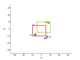
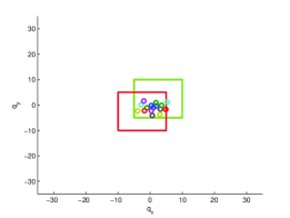
Figure 15: The trajectories of the generalized coordinates of the agents under control (13). The circles denote the generalized coordinates of the agents. The agents converge to the fixed points in the intersection of the local target sets.

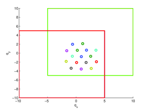
Figure 16: Zoom in of the final generalized coordinates of the agents under control (13).

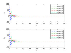
Figure 17: The trajectories of the generalized coordinate derivatives of the agents under control (13).

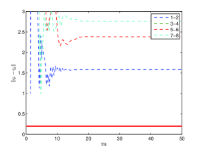
Figure 18: The trajectories of the relative generalized coordinates of the agents under control (13). The solid line denotes the minimum safety distance.

V-B2 Complete graph

we next consider the case when the communication graph is a complete graph. The communication weight is chosen to be $1$.

Under the control (13), snapshots of generalized coordinates and trajectories of generalized coordinate derivatives of the agents are shown in Figs. 19, 20 and 21. Also, the trajectories of the relative generalized coordinates of the agents is shown in Fig. 22. We see that set aggregation is achieved while collision avoidance is guaranteed. Obviously, in this case, all the agents converge to a region that is more tight than that of the case of star graph. The comparisons between the cases of star graph and complete graph suggest that the sparse communication connections are more effective for the coverage of interested tracking region.

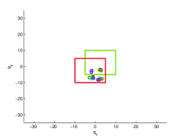
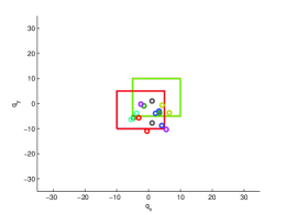
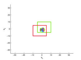
Figure 19: The trajectories of the generalized coordinates of the agents under control (13). The circles denote the generalized coordinates of the agents. The agents converge to the fixed points in the intersection of the local target sets.

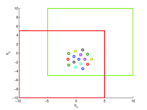
Figure 20: Zoom in of the final generalized coordinates of the agents under control (13).

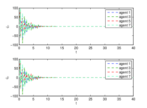
Figure 21: The trajectories of the generalized coordinate derivatives of the agents under control (13).

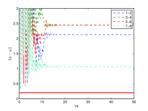
Figure 22: The trajectories of the relative generalized coordinates of the agents under control (13). The solid line denotes the minimum safety distance.

V-C Discussions on Switching Communication Graphs

An analytical investigation for jointly switching communication and collision avoidance is difficult. The conceptual reasons include

1. There is no equilibrium point for this case and therefore generalized coordinate derivative consensus cannot be achieved. Consequently, the generalized coordinates of the agents will not converge to a steady state.

2. Even to show the boundedness of the agent generalized coordinate derivatives and the distances between $q_{i}$, $i\in\mathcal{V}$ and the intersection of local target sets encounters some fundamental difficulties. The reason for this is that it is hard to find an appropriate Lyapunov function to capture both the time-varying collision avoidance term and the switching communication graph simultaneously.

We next illustrate the open problem discussed above using simulations. We consider the case that the communication graph is switching between a star graph (connected graph) and a complete graph (connected graph) every five seconds (uniformly). Under the control law (13), snapshots of generalized coordinates and trajectories of generalized coordinate derivatives of the agents are shown in Figs. 23 and 24. Note that the agents do not converge to steady state, but instead, the formation of the agents expands and contracts periodically. Moreover, note that the generalized coordinate derivatives of the agents do not converge to zero. Therefore, approximate aggregation is not achieved in general when the communication graphs are switching. To understand this complex dynamical behavior is an interesting topic for further research.

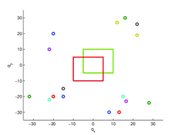
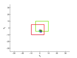
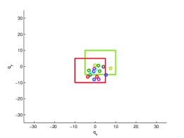
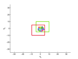
Figure 23: The trajectories of the generalized coordinates of the agents under control (13). The circles denote the generalized coordinates of the agents. The agent behaviors converge to an contraction-expansion oscillation.

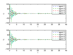
Figure 24: The trajectories of the generalized coordinate derivatives of the agents under control (13).

VI Conclusions

In this paper, we study cooperative set aggregation of multiple Lagrangian systems. The objective is to drive multiple Lagrangian systems to approach a common set while each system has only access to the constrained information on this common set. By exchanging information with neighboring agents, we first show that all the Lagrangian systems converge to the intersection of all the local available sets under both fixed and switching communication graphs. Moreover, we introduce collision avoidance control term to ensure collision avoidance. By defining an ultimate bound on the final generalized coordinates between each system and the intersection of all the local available sets, we show that the set aggregation under collision avoidance is achieved while the generalized coordinate derivatives of all the systems are driven to zero. Simulation results are given to validate the theoretical results.

References

- [1] T. Vicsek, A. Czirok, E. B. Jacob, I. Cohen, and O. Schochet, “Novel type of phase transitions in a system of self-driven particles,” Physical Review Letters, vol. 75, no. 6, pp. 1226–1229, 1995.
- [2] Z. Lin, M. Broucke, and B. Francis, “Local control strategies for groups of mobile autonomous agents,” IEEE Transactions on Automatic Control, vol. 49, no. 4, pp. 622–629, 2004.
- [3] M. M. Zavlanos and G. J. Pappas, “Distributed connectivity control of mobile networks,” IEEE Transactions on Robotics, vol. 24, no. 6, pp. 1416–1428, 2008.
- [4] G. Hollinger, S. Singh, and A. Kehagias, “Improving the efficiency of clearing with multi-agent teams,” The International Journal of Robotics Research, vol. 29, no. 8, pp. 1088–1105, 2010.
- [5] F. Bullo, E. Frazzoli, M. Pavone, K. Savla, and S. Smith, “Dynamic vehicle routing for robotic systems,” Proceedings of the IEEE, vol. 99, no. 9, pp. 1482–1504, 2011.
- [6] R. Aragues, J. Cortes, and C. Sagues, “Distributed consensus on robot networks for dynamically merging feature-based maps,” IEEE Transactions on Robotics, vol. 28, no. 4, pp. 840–854, 2012.
- [7] A. Canedo-Rodriguez, C. Regueiro, R. Iglesias, V. Alvarez-Santos, and X. Pardo, “Self-organized multi-camera network for ubiquitous robot deployment in unknown environments,” Robotics and Autonomous Systems, vol. 61, no. 7, pp. 667–675, 2013.
- [8] A. Franchi, G. Oriolo, and P. Stegagno, “Mutual localization in multi-robot systems using anonymous relative measurements,” The International Journal of Robotics Research, vol. 32, no. 11, pp. 1302–1322, 2013.
- [9] A. Jadbabaie, J. Lin, and A. S. Morse, “Coordination of groups of mobile autonomous agents using nearest neighbor rules,” IEEE Transactions on Automatic Control, vol. 48, no. 6, pp. 988–1001, 2003.
- [10] R. Olfati-Saber, J. A. Fax, and R. M. Murray, “Consensus and cooperation in networked multi-agent systems,” Proceedings of the IEEE, vol. 95, no. 1, pp. 215–233, 2007.
- [11] M. Cao, A. S. Morse, and B. D. O. Anderson, “Agreeing asynchronously,” IEEE Transactions on Automatic Control, vol. 53, no. 8, pp. 1826–1838, 2008.
- [12] A. Ganguli, J. Cortes, and F. Bullo, “Multirobot rendezvous with visibility sensors in nonconvex environments,” IEEE Transactions on Robotics, vol. 25, no. 2, pp. 340–352, 2009.
- [13] K. D. Do, “Coordination control of underactuated ODINs in three-dimensional space,” Robotics and Autonomous Systems, vol. 61, no. 8, pp. 853–867, 2013.
- [14] F. Pasqualetti, J. W. Durham, and F. Bullo, “Cooperative patrolling via weighted tours: Performance analysis and distributed algorithms,” IEEE Transactions on Robotics, vol. 28, no. 5, pp. 1181–1188, 2012.
- [15] R. Olfati-Saber and R. M. Murray, “Consensus problems in networks of agents with switching topology and time-delays,” IEEE Transactions on Automatic Control, vol. 49, no. 9, pp. 1520–1533, 2004.
- [16] W. Ren and R. W. Beard, “Consensus seeking in multiagent systems under dynamically changing interaction topologies,” IEEE Transactions on Automatic Control, vol. 50, no. 5, pp. 655–661, 2005.
- [17] L. Moreau, “Stability of multi-agent systems with time-dependent communication links,” IEEE Transactions on Automatic Control, vol. 50, no. 2, pp. 169–182, 2005.
- [18] Z. Lin, B. Francis, and M. Maggiore, “State agreement for continuous-time coupled nonlinear systems,” SIAM Journal of Control and Optimization, vol. 46, no. 1, pp. 288–307, 2007.
- [19] F. Dorfler, M. Chertkov, and F. Bullo, “Synchronization in complex oscillator networks and smart grids,” Proceedings of the National Academy of Sciences, vol. 110, no. 6, pp. 2005–2010, 2013.
- [20] W. Ren, “Distributed leaderless consensus algorithms for networked Euler-Lagrange systems,” International Journal of Control, vol. 82, no. 11, pp. 2137–2149, 2009.
- [21] S.-J. Chung and J.-J. E. Slotine, “Cooperative robot control and concurrent synchronization of Lagrangian systems,” IEEE Transations on Robotics, vol. 25, no. 3, pp. 686–700, 2009.
- [22] D. V. Dimarogonas and K. J. Kyriakopoulos, “Connectedness preserving distributed swarm aggregation for multiple kinematic robots,” IEEE Transactions on Robotics, vol. 24, no. 5, pp. 1213–1223, 2008.
- [23] S. Khoo, L. Xie, and Z. Man, “Robust finite-time consensus tracking algorithm for multirobot systems,” IEEE/ASME Transcations on Mechatronics, vol. 14, no. 2, pp. 219–228, 2009.
- [24] J. Mei, W. Ren, and G. Ma, “Distributed containment control for Lagrangian networks with parametric uncertainties under a directed graph,” Automatica, vol. 48, no. 4, pp. 653–659, 2012.
- [25] G. Chen and F. L. Lewis, “Distributed adaptive tracking control for synchronization of unknown networked Lagrangian systems,” IEEE Transcations on Systems, Man and Cybernetics-Part B: Cybernetics, vol. 41, no. 3, pp. 805–816, 2011.
- [26] Z. Meng, Z. Lin, and W. Ren, “Leader-follower swarm tracking for networked Lagrange systems,” Systems and Control Letters, vol. 61, no. 1, pp. 117–126, 2012.
- [27] R. Haghighi and C. C. Cheah, “Multi-group coordination control for robot swarms,” Automatica, vol. 48, no. 10, pp. 2526–2534, 2012.
- [28] Y.-C. Liu and N. Chopra, “Controlled synchronization of heterogeneous robotic manipulators in the task space,” IEEE Transactions on Robotics, vol. 28, no. 1, pp. 268–275, 2012.
- [29] J.-P. Aubin, Viability Theory. Birkhauser Boton, Boston, 1991.
- [30] C. Godsil and G. Royle, Algebraic Graph Theory. New York: Springer-Verlag, 2001.
- [31] A. F. Filippov, Differential Equations with Discontinuous Righthand Sides. Norwell, MA: Kluwer, 1988.
- [32] J. M. Danskin, “The theory of max-min, with applications,” SIAM Journal on Applied Mathematics, vol. 14, no. 4, pp. 641–664, 1966.
- [33] M. W. Spong, S. Hutchinson, and M. Vidyasagar, Robot dynamics and control. John Wiley & Sons, Inc., 2006.
- [34] L. G. Gubin, B. T. Polyak, and E. V. Raik, “The method of projections for finding the common point of convex sets,” USSR Computational Mathematics and Mathematical Physics, vol. 7, no. 6, pp. 1211–1228, 1967.
- [35] A. Nedic, A. Ozdaglar, and P. A. Parrilo, “Constrained consensus and optimization in multi-agent networks,” IEEE Transactions on Automatic Control, vol. 55, no. 4, pp. 922–938, 2010.
- [36] G. Shi, K. H. Johansson, and Y. Hong, “Reaching an optimal consensus: dynamical systems that compute intersections of convex sets,” IEEE Transactions on Automatic Control, vol. 58, no. 3, pp. 610–622, 2013.
- [37] H. K. Khalil, Nonlinear Systems, Third Edition. Englewood Cliffs, New Jersey: Prentice-Hall, 2002.
- [38] D. Liberzon and A. S. Morse, “Basic problems in stability and design of switched systems,” IEEE Control Systems Magazine, vol. 19, no. 5, pp. 59–70, 1999.
- [39] P. F. Hokayem, D. M. Stipanovic, and M. W. Spong, “Coordination and collision avoidance for lagrangian systems,” Applied Mathematics and Computation, vol. 217, no. 3, pp. 1085–1094, 2010.
- [40] F. Deutscha and H. Hundal, “The rate of convergence for the cyclic projections algorithm III: Regularity of convex sets,” Journal of Approximation Theory, vol. 155, no. 2, pp. 155–184, 2008.