CMB Polarization Anisotropies as a Probe of Primordial Gravity Waves Generated by Inflation

HALF-WAVE PLATES FOR THE SPIDER COSMIC MICROWAVE BACKGROUND POLARIMETER

by
SEAN ALAN BRYAN
Submitted in partial fulfillment of the requirements
for the degree of Doctor of Philosophy

Dissertation Adviser: Dr. John Ruhl

Department of Physics
CASE WESTERN RESERVE UNIVERSITY
May, 2014

CASE WESTERN RESERVE UNIVERSITY
SCHOOL OF GRADUATE STUDIES

© 2014, Sean Bryan

For my family.

The Spider Team

P. A. R. Ade,¹ M. Amiri,² S. J. Benton,³ R. F. Bihary,⁴ J. J. Bock,^5,6 J. R. Bond,⁷ J. A. Bonetti,⁶ S. Bryan,⁴ H. C. Chiang,⁸ C. R. Contaldi,⁹ B. P. Crill,^5,6 O. Dore,^5,6 M. Farhang,^7,3 J. P. Filippini,⁵ L. M. Fissel,^10,3 A. A. Fraisse,¹¹ A. Gambrel,¹¹ N. N. Gandilo,¹² J. E. Gudmundsson,¹¹ M. Halpern,² M. Hasselfield,^13,2 G. Hilton,¹⁴ W. Holmes,⁶ V. V. Hristov,⁵ K. Irwin,¹⁵ W. C. Jones,¹¹ Z. K. Kermish,¹¹ C. J. MacTavish,¹⁷ P. V. Mason,⁵ L. Moncelsi,⁵ T. E. Montroy,⁴ T. A. Morford,⁵ J. M. Nagy,⁴ C. B. Netterfield,^3,12 A. S. Rahlin,¹¹ C. Reintsema,¹⁴ J. E. Ruhl,⁴ M. C. Runyan,⁶ J. A. Shariff,¹² J. D. Soler,^17,12 A. Trangsrud,⁵ C. Tucker,¹ R. S. Tucker,⁵ A. D. Turner,⁶ A. C. Weber,⁶ D. Wiebe,² and E. Young,¹¹

¹School of Physics and Astronomy, Cardiff University, Cardiff, UK
²Department of Physics and Astronomy, University of British Columbia, Vancouver, BC, Canada
³Department of Physics, University of Toronto, Toronto, ON, Canada
⁴Department of Physics, Case Western Reserve University, Cleveland, OH, USA
⁵Division of Physics, Mathematics & Astronomy, California Institute of Technology, Pasadena, CA, USA
⁶Jet Propulsion Laboratory, Pasadena, CA, USA
⁷Canadian Institute for Theoretical Astrophysics, University of Toronto, Toronto, ON, Canada
⁸School of Mathematics, Statistics & Computer Science, University of KwaZulu-Natal, Durban, South Africa
⁹Theoretical Physics, Blackett Laboratory, Imperial College, London, UK
¹⁰CIERA- Northwestern University, Evanston, IL, USA
¹¹Department of Physics, Princeton University, Princeton, NJ, USA
¹²Department of Astronomy and Astrophysics, University of Toronto, Toronto, ON, Canada
¹³Department of Astrophysical Sciences, Princeton University, Princeton, NJ, U.S.A
¹⁴National Institute of Standards and Technology, Boulder, CO, USA
¹⁵Department of Physics, Stanford University, Stanford, CA, U.S.A.
¹⁶Kavli Institute for Cosmology, University of Cambridge, Cambridge, U.K.
¹⁷Institut d’Astrophysique Spatiale IAS, CNRS & Université Paris-Sud, Orsay Cedex, France

Half-wave Plates for the Spider
Cosmic Microwave Background Polarimeter
by

SEAN ALAN BRYAN

Abstract

Spider is a balloon-borne array of six telescopes that will observe the Cosmic Microwave Background. The 2400 antenna-coupled bolometers in the instrument will make a polarization map of the CMB with $\sim$degree resolution at 150 GHz and 95 GHz. Polarization modulation is achieved via a cryogenic sapphire half-wave plate (HWP) skyward of the primary optic. In this thesis, the design, construction, and lab testing of the HWP system are discussed. The polarization modulation of these optical stacks is modeled using a physical optics calculation and Mueller matrices. Performance tests in both the lab and integrated in the flight cryostat show consistency with the model.

Chapter 1 Introduction

One of the key frontiers in modern cosmology is measuring the temperature and polarization anisotropies of the Cosmic Microwave Background (CMB) radiation. The anisotropies encode a wealth of information about inflation [baumann09], re-ionization [zaldarriaga08], and the large-scale structure of the universe [smith08]. From the discovery of the CMB in 1965 by Penzias and Wilson [penzias65] through to the Planck satellite of today [planck13a], measurements of the CMB have been a key ingredient in establishing the standard model of cosmology.

The CMB is relic light from the early universe. The temperature of the universe before $t\sim 380,000$ years after the Big Bang was high enough that the universe was filled with a plasma of coupled photons and charged particles. As the universe expanded and cooled, neutral hydrogen formed, capturing the free electrons. This event, called recombination, allowed the photons to travel without scattering electromagnetically. This free-streaming background of photons is the CMB that we observe today. Structure in the universe from that era is imprinted on the CMB as hot and cold spots, which means the CMB is the oldest direct picture of the universe we have. The CMB is sometimes called the “smoking gun” of the Hot Big Bang scenario.

The uniformity of the CMB temperature across the sky actually presents a challenge to the Hot Big Bang scenario as it was originally conceived. The largest volume of the universe that could have been in causal contact at the time of recombination has an apparent angular size of today of $\sim 2^{\circ}$. However, the CMB temperature is highly uniform across the entire sky, to better than one part in $10^{4}$. This paradox is called the Horizon Problem. Inflation, conceived by Guth [guth81] and independently by Starobinsky [starobinsky80], postulates that there was an early time in the universe’s history when the universe expanded exponentially, growing a small causally-connected volume in the pre-inflation era into a large enough volume to explain the uniformity of the CMB. Quantum fluctuations in the field driving the inflationary expansion seeded density perturbations that later grew through gravitational collapse into the fluctuations seen in the CMB, and much later grew into the large-scale structure of the universe today. The quantum fluctuations also perturbed the rest of the metric to create a background of gravitational waves that left an imprint on the polarization of the CMB. Precision measurements of the CMB temperature and polarization are therefore a powerful probe to learn about the physics of inflation.

1.1 CMB Polarization

1.1.1 Physical Origin

Once the dipole due to the proper motion of the earth is subtracted, the CMB has temperature anisotropies at the $\sim 100~{}\mu$K level, about 4 parts in $10^{5}$ [hu97]. These were generated by temperature variations in the plasma, Doppler shifts due to motion of the plasma along our line of sight, and redshifting of photons as they climb out of potential wells formed by overdensities and underdensities of Dark Matter. The plasma also generated linearly-polarized light through Thomson scattering. In Thomson scattering, photons scatter off electrons, and the differential cross section is

$$\frac{d\sigma}{d\Omega}=\frac{3\sigma_{T}}{8\pi}{|\hat{\epsilon}^{\prime}\cdot\hat{\epsilon}|}^{2},$$ (1.1)

where $\hat{\epsilon}^{\prime}$ and $\hat{\epsilon}$ are unit vectors in the direction of the scattered and incident photons respectively. The incident electromagnetic wave causes the electron to move. Accelerating charge radiates, so light is re-emitted with a directional dependence governed by the Thomson cross section.

The CMB photons we observe today were emitted along a line of sight to us from the spherical surface of last scattering. Light incident on a small volume of plasma from the last-scattering surface causes the electrons in that plasma patch to move and radiate out to us in the line-of-sight direction. If the plasma is surrounded by an isotropic field of photons, the E-field amplitudes incident along the last scattering surface will be equal, and the radiation in the line-of-sight direction will be unpolarized. As illustrated in Figure 1.1, if the plasma is surrounded by a field of photons with a quadrupolar brightness distribution (generated by density perturbations or gravity waves), the E-field amplitudes coming from one direction will be higher than those waves from the orthogonal direction. This causes the radiation in the line-of-sight direction towards us to be partially polarized.

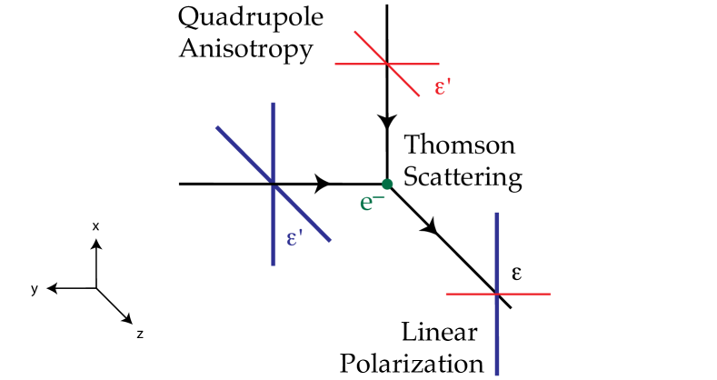
Figure 1.1: A local quadrupole generates linear polarization. The light incident on the electron is from a cooler source in the vertical direction, and a warmer source in the horizontal direction. This causes the scattered light to be partially polarized. Figure from Hu and White [hu97].

Since they naturally describe partially polarized incoherent light, we use the Stokes Parameters to characterize the polarization state of light of the CMB. For light traveling in the $z$ direction, these are defined in [hecht74] as

$$I = <a_{x}^{2}>+<a_{y}^{2}>$$ (1.2)

$$Q = <a_{x}^{2}>-<a_{y}^{2}>$$ (1.3)

$$U = <2a_{x}a_{y}\cos{(\theta_{x}-\theta_{y})}>$$ (1.4)

$$V = <2a_{x}a_{y}\sin{(\theta_{x}-\theta_{y})}>,$$ (1.5)

where

$$E_{x} = a_{x}(t)\cos{(kz-\omega t-\theta_{x}(t))}$$ (1.6)

$$E_{y} = a_{y}(t)\cos{(kz-\omega t-\theta_{y}(t))}$$ (1.7)

are the $x$ and $y$ components of the electric fields, and the $<>$ operator indicates averaging over a timescale much longer than $1/\omega$. The physical interpretations of the Stokes Parameters are $I$ $\sim$ intensity, $Q,U$ $\sim$ linear polarization, and $V$ $\sim$ circular polarization. For example $(I,Q,U,V)=(1,0,0,0)$ is completely unpolarized light, $(1,1,0,0)$ is completely linearly polarized light, and $(1,0.5,0,0)$ is partially linearly polarized light. Thomson scattering only produces linear polarization, so $V=0$ for the CMB. This means that light from the CMB can be characterized as a pseudo-vector with polarization fraction $\sqrt{Q^{2}+U^{2}}/I$ and polarization angle $\frac{1}{2}$atan2${(U,Q)}$. Here $\mathrm{atan2}$ is the two-argument arctangent function that returns a signed angle, indicating the rotation direction. It is defined as

$$\mathrm{atan2}(y,x)\equiv 2\tan^{-1}{\frac{y}{\sqrt{x^{2}+y^{2}}+x}}.$$ (1.8)

A full-sky map of the polarization anisotropy of the CMB can therefore be visualized as a pseudo-vector field on the surface of the sphere.

At angular scales larger than $~{}\sim 1^{\circ}$, the two dominant sources of polarization anisotropies are density perturbations and gravity waves. These two kinds of perturbations differ in their transformation properties under global parity flips. For a field defined in a plane, a global parity flip is equivalent to looking at the field in a mirror. This picture can be generalized to a sphere, since a sphere is locally flat around any point. The density perturbations generate a polarization field $\vec{P}(\hat{n})$, where $\hat{n}=(\theta,\phi)$ is a unit vector pointing to a direction on the sky. Since density is a scalar quantity, this polarization field must be invariant under a global parity flip. It follows that the field $\vec{P}(\hat{n})$ must have a vanishing curl. By analogy with electromagnetism, polarization patterns with a vanishing curl are called E-modes.

Gravity waves also generate local quadrupoles in temperature, and therefore generate polarization. Considering a spherical patch of plasma, a passing gravity wave would induce an elliptical distortion. This would compress and heat the plasma along one direction, and rarefy and cool the plasma along the orthogonal direction. This would induce a quadrupolar brightness distribution, and therefore would radiate partially polarized light as illustrated in Figure 1.1. Since gravity waves are tensors, the gravity wave perturbations need not be invariant under a global parity flip, so the polarization field they generate need not be invariant. This implies that the $\vec{P}(\hat{n})$ generated by this mechanism can contain a non-zero curl. Again by analogy with electromagnetism, polarization patterns with curl are called B-modes. The only physical mechanism that can generate B-modes at the surface of last scattering is a background of gravity waves. Because of their global transformation properties, density perturbations (scalars) produce only E-modes, and gravity waves (tensors) produce roughly equal amounts of E- and B-modes. Detecting B-modes at large angular scales is therefore a detection of the primordial gravity waves in the universe at the time of last scattering.

1.1.2 Angular Power Spectra

Angular power spectra can be calculated from maps of the CMB temperature and polarization for comparison with theory and constraining cosmological parameters. The spherical harmonic functions $Y_{l}^{m}$ are the basis for estimating the angular power spectrum of the CMB, since the maps are on the surface of a sphere. For the temperature maps, $C_{l}^{\mathrm{TT}}$ are the spherical harmonic coefficients when the temperature map is decomposed onto spherical harmonics and the $a_{lm}$’s are combined according to

$$C_{l}^{\mathrm{TT}}=<a_{lm}a_{lm}^{*}>,$$ (1.9)

where the brackets denote an average over $m$. This decomposition works if the ordinary spin-0 spherical harmonics are used, since temperature is a scalar quantity.

Because polarization maps transform under global parity flips and rotations as spin-2 objects, polarization maps may be expressed using the spin-2 spherical harmonic functions as a basis [balbi06]. The maps are expressed as

$$Q(\hat{n})+iU(\hat{n})=\sum_{l>0}\sum_{m=-l}^{l}(a_{lm}^{E}+ia_{lm}^{B})Y_{l}^{m}(\hat{n}),$$ (1.10)

where $Y_{l}^{m}$ are the spin-2 spherical harmonics, not the ordinary spin-0 spherical harmonics. In the convention used in [page07], the $C_{l}$ are calculated with

$$C_{l}^{\mathrm{XY}}=<a_{lm}^{X}a_{lm}^{Y*}>.$$ (1.11)

Here X and Y are T (temperature), E (E-modes), or B (B-modes). The possible spectra to calculate from a given observation are the temperature spectrum $C_{l}^{\mathrm{TT}}$, the temperature-polarization cross spectra $C_{l}^{\mathrm{TE}}$ and $C_{l}^{\mathrm{TB}}$, and the polarization spectra $C_{l}^{\mathrm{EB}}$, $C_{l}^{\mathrm{EE}}$ and $C_{l}^{\mathrm{BB}}$.

All of these measured angular power spectra can be compared with calculated values of the theoretical angular power spectrum. The TT, EE, and BB spectra can all be non-zero, since they are auto-correlations. The review in Hu and White [hu97] shows that because of how E- and B-modes transform under parity, the TE spectrum is non-zero but TB and EB are identically zero. TB and EB can appear to be non-zero if there is a global rotation of all of the polarization directions from cosmic birefringence, or due to incorrect calibration of the detector sensitivity angles [keating13].

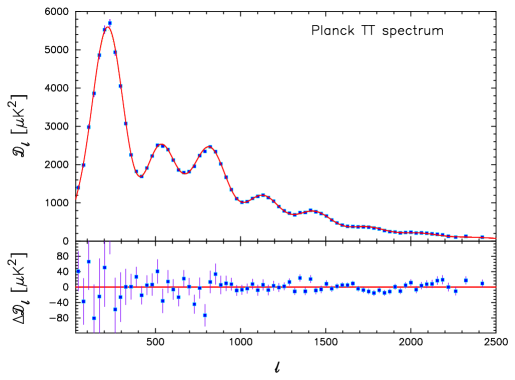
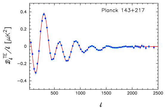
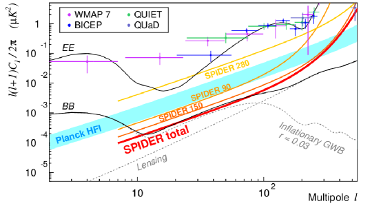
Figure 1.2: Planck TT and TE spectra, EE spectra from several experiments, and expected Spider BB sensitivity per multipole $l$. This projection assumes a first flight with 3x 95 GHz receivers, and 3x 150 GHz receivers, and a second flight with 2 receivers each at 95 GHz, 150 GHz, and 280 GHz. From Planck [planck13b] and Fraisse et al. [fraisse13] .

1.2 Inflation

1.2.1 Horizon Problem

The CMB is remarkably homogeneous, suggesting that the entire currently observable universe was once in causal contact and thermal equilibrium. It turns out that in the Hot Big Bang scenario, there never was such a time! This paradox is the Horizon Problem. Ryden [ryden03] reviews the problem as follows. The horizon distance at the time of last scattering is calculated to be $d_{\mathrm{hor}}(t_{\mathrm{ls}})\approx 0.27~{}\mathrm{Mpc}$ in the Standard Model, and the angular-diameter distance to the surface of last scattering is calculated to be $d_{A}\approx$ 13 Mpc. This means that a causally-connected region of space at the time of last scattering has an apparent angular size today of

$$\theta_{\mathrm{apparent}}=\frac{2d_{\mathrm{hor}}(t_{\mathrm{ls}})}{d_{A}}\approx\frac{0.53~{}\mathrm{Mpc}}{13~{}\mathrm{Mpc}}\approx 2^{\circ}.$$ (1.12)

This means that in the Hot Big Bang model, the CMB should not appear isotropic on scales larger than $2^{\circ}$. However, the entire sky is uniformly $2.7$ K, to about four parts in $10^{5}$. This means there must have been some event in the early universe that caused the currently observable universe to be in causal contact.

Inflation solves this problem by postulating a period in which the universe was briefly dominated for a time $t_{\mathrm{inflation}}$ by a component with an equation of state $w<1/3$. For a cosmological constant, $w=-1$, and the scale factor grows exponentially with time during this period:

$$a(t)\propto e^{Ht}.$$ (1.13)

In grand unified theories (GUT) of particle physics, in order to solve the monopole problem (i.e. the non-detection of monopoles today, despite their calculated abundant production in the early universe in grand unified theories of particle physics), inflation must have started after the temperature of the universe was at the GUT scale, $\sim 10^{16}$ GeV. Since the universe was radiation-dominated at the GUT time, the horizon distance just before inflation was $d_{\mathrm{hor}}(t_{\mathrm{before}})=2ct_{\mathrm{before}}$. Ryden shows that just after inflation, the horizon size at the end of inflation expanded to

$$d_{\mathrm{hor}}(t_{\mathrm{before}}+t_{\mathrm{inflation}})=e^{N}c(2t_{\mathrm{before}}+H_{\mathrm{before}}^{-1})\approx e^{N}3ct_{\mathrm{before}},$$ (1.14)

where $N\equiv Ht_{\mathrm{inflation}}$ is the number of e-folds of inflation. After inflation, this horizon keeps growing according to the usual radiation-driven, matter-driven, then cosmological-constant-driven expansion history of the universe from then to the present day. For inflation at the GUT scale, $N\geq 60$ is required to solve the horizon problem.

1.2.2 Perturbations

Inflation was conceived to solve the monopole problem and the horizon problem, but it makes other testable predictions. If inflation is driven by a scalar field $\phi$ with a potential $V(\phi)$, the value of this field will vary spatially due to quantum fluctuations. Inflation expands these virtual quantum fluctuations to scales larger than the horizon, which turns them into real macroscopic perturbations. At the end of inflation, the scalar field will decay into dark matter, baryons, photons, and all of the other Standard Model particles. This means that the fluctuations in the inflaton field will decay into density fluctuations in the baryon-photon plasma and dark matter. Measuring these fluctuations in cosmological observables is a way to directly probe the physics of inflation.

Measurements of the large-scale temperature anisotropies of the CMB give a measurement of the overall amplitude of the primordial density perturbations. If inflation was the mechanism that generated these perturbations, the review by Liddle and Lyth [liddle00] shows that this in turn is a constraint on the quantity $(V/\epsilon)^{\frac{1}{4}}$, where

$$\epsilon\equiv\frac{m_{\mathrm{p}}^{2}}{16\pi}\left(\frac{V^{\prime}}{V}\right)^{2}$$ (1.15)

is one of the slow-roll parameters. The current value of this constraint is given in [baumann09] as $(V/\epsilon)^{\frac{1}{4}}\approx 6.30\times 10^{16}$ GeV.

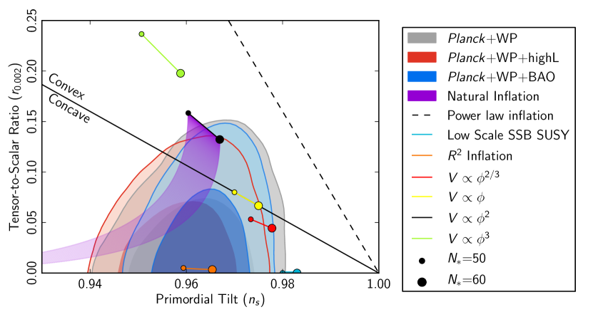
Figure 1.3: Both $n_{s}$ and $r$ can constrain inflationary models. The plot above shows the constraints from Planck [planck13b] and other experiments, overlaid with predictions for several inflationary models. The vertical axis shows constraints on $r_{0.002}$, which is the tensor-to-scalar ratio $r$ measured at $k=0.002~{}\mathrm{Mpc}^{-1}$.

Just as inflation causes density perturbations, it also perturbs the entire metric $\tilde{g}_{\mu\nu}=g_{\mu\nu}+h_{\mu\nu}$, where $g_{\mu\nu}$ is the background Friedmann-Robertson-Walker metric. Taking $h$ to be small means the perturbations are linear. Following the review in Peacock [peacock99], the RMS amplitude of the gravity wave (tensor) perturbations are $h_{\mathrm{rms}}\sim H/m_{\mathrm{p}}$, small enough for linear theory. Assuming inflation is driven by a simple scalar field, quantum field theory can be used to calculate the ratio $r$ of the amplitude of the tensor perturbations $\Delta_{\mathrm{T}}$ to the amplitude of the scalar perturbations $\Delta_{\mathrm{S}}$. The result is

$$\frac{\Delta_{\mathrm{T}}^{2}}{\Delta_{\mathrm{S}}^{2}}\equiv r\approx 12.4\epsilon.$$ (1.16)

Combining this result with the bound on $(V/\epsilon)^{\frac{1}{4}}$ yields a relationship between $r$ and the energy scale of inflation $V^{\frac{1}{4}}$, given in [baumann09] as

$$E_{inflation}\equiv V^{\frac{1}{4}}=1.06\times 10^{16}~{}\mathrm{GeV}~{}\left(\frac{r}{0.01}\right)^{\frac{1}{4}}.$$ (1.17)

This means that a measurement of $r$ would be a measurement of the energy scale of inflation.

Measurements of the spectrum of the primordial density perturbations also constrain inflation. Continuing the calculation presented in [peacock99], in inflation the scalar spectral index $n_{s}$ is calculated to deviate from scale invariance ($n_{s}=1$) by

$$1-n_{s}=6\epsilon-2\eta,$$ (1.18)

where

$$\eta\equiv\frac{m_{\mathrm{p}}^{2}}{8\pi}\left(\frac{V^{\prime\prime}}{V}\right)$$ (1.19)

is the other slow-roll parameter. For typical polynomial potentials, $\eta\sim\epsilon$, so inflation generically predicts that $r$ and $n_{s}$ will be related by

$$r\approx 3(1-n_{s}).$$ (1.20)

Planck has measured that $(1-n_{s})=0.0376\pm 0.0075$ [planck13a], so single-field power-law-potential inflation generically predicts $r\sim 0.1$. It is of course possible to come up with a model of inflation with a different relationship among the primordial perturbation, $r$ and $n_{s}$, which could result in a vanishingly small $r$. Predictions for $r$ and $n_{s}$ in two such models are also shown in Figure 1.3.

The best current upper limits on $r$ come indirectly from the large-angle CMB temperature spectrum. If $r$ were large enough, the tensor perturbations would induce temperature anisotropies at large angular scales in the CMB, so the current non-detection of excess anisotropies at large angular scales sets a limit of $r<0.1$ at $95\%$ confidence [planck13a]. Since those measurements have low enough instrument noise now that they are cosmic-variance limited, current upper limits on $r$ will not improve significantly with improved temperature measurements. However, the BB polarization spectrum directly gives a measurement of $r$. Figure 1.3 shows the current observational constraints on $n_{s}$ and $r$ along with predictions from several models of inflation. According to simulations [fraisse13], after two flights the BB measurements of Spider will detect or set an upper limit on $r$ of 0.03 at $99\%$ confidence, which would detect or rule out the simple $V\sim\phi^{N}$ models of inflation shown in the figure.

1.3 Observing B-modes in the CMB

1.3.1 Primordial B-mode Signal

The gravity wave background generated by inflation induces a B-mode polarization pattern at the surface of last scattering, a signal that would peak at roughly $l=100$ as shown in Figure 1.2. This is the signal Spider is hunting for. The peak appears at large enough angular scales that the roughly half-degree beam sizes in Spider are enough to resolve the feature. As discussed further in Section LABEL:spider_scan, the feature appears on small enough angular scales that we can concentrate the sensitivity of the instrument on a relatively small observing region, roughly $10\%$ of the sky. Also, the scan speed of the instrument will put this signal at roughly 1 Hz in the detector timestreams, which is a high enough frequency that the detector drifts will not be a problem, and low enough to be well below the time constant of the detectors.

Later in the history of the universe, between redshifts of 10 and 5, the neutral hydrogen in the universe was reionized, creating a diffuse population of charged particles. Light from the CMB Thomson-scattered from the electrons in this plasma, creating E- and B-mode polarization patterns that we could observe today. This signal appears on very large angular scales, roughly $l<10$. Searching for this signal would require mapping a larger fraction of the sky than is available to Spider observing during its Antarctic flight. Also, as discussed in Section 1.3.3, foreground contamination is higher at large angular scales, which would present an additional challenge to searching for this signal.

1.3.2 Lensing B-mode Signal

Gravitational lensing by large-scale structure distorts the primordial temperature and polarization anisotropies of the CMB as they travel to us from the surface of last scattering. As reviewed in [smith08], lensing takes the primordial maps emitted by the surface of last scattering $[I(\hat{n}),Q(\hat{n}),U(\hat{n})]$ and deflects the rays as they travel to us to form the lensed maps $[I(\hat{n}+\nabla\varphi(\hat{n})),Q(\hat{n}+\nabla\varphi(\hat{n})),U(\hat{n}+\nabla\varphi(\hat{n}))]$ that we observe. The angular power spectrum of this lensing deflection field $\varphi(\hat{n})$ is approximately

$$C_{l}^{\varphi\varphi}=\frac{8\pi^{2}}{l^{3}}\int_{0}^{z_{rec}}\frac{dz}{H(z)}D(z)\left(\frac{D(z_{rec})-D(z)}{D(z_{rec})D(z)}\right)^{2}P_{\psi}(z,k=l/D(z)),$$ (1.21)

where $z_{rec}$ is the redshift of recombination, $D$ is the comoving distance to redshift $z$ and $P_{\psi}$ is the power spectrum of the gravitational potential generated by large-scale structure. This relation shows that measuring the lensing deflection field is a measurement of both the growth of structure in the recent $z\,\hbox{\lower 2.58334pt\hbox{$\sim$}\hbox to0.0pt{\hss\raise 2.58334pt\hbox{$<$}}}\,5$ universe ($P_{\psi})$ and the expansion rate of the recent universe (encoded in $H(z)$ and $D(z)$).

A natural basis for analyzing polarization data in search of the lensing signal is to use an estimator optimized to measure the deflection field $\varphi(\hat{n})$, its angular power spectrum $C_{l}^{\varphi\varphi}$, or its correlation with other measurements. However, thinking instead in the usual E-mode and B-mode decomposition, lensing induces a B-mode signal by distorting the primordial E-mode signal. This lensing B-mode signal is shown in Figure 1.2 overplotted in the same panel that shows the expected B-mode sensitivity of Spider. The signal is expected to peak near $l\approx 1000$, and its expected amplitude is calculable from existing measurements of large-scale structure. The signal was recently detected by the SPTpol instrument [hanson13]. On angular scales smaller than $l\approx 90$, B-modes generated by lensing are larger than the primordial $r=0.03$ B-mode signal that Spider is searching for. At all scales, the lensing signal is below the sensitivity of Spider, so we believe that confusion between lensing and primordial B-modes will not limit our results. Future experiments searching for primordial B-modes well below $r\sim 0.01$ may need to “delens” their maps by measuring the lensing deflection field in their maps and removing its effects before hunting for the primordial $r$ signal in their data.

1.3.3 Dust Foreground Removal

The dominant foreground in Spider’s frequency bands and observing region is expected to be polarized dust emission from our galaxy. Since other instruments have not yet made low-noise polarized maps at Spider’s observing frequencies in this part of the sky, there is not existing data on the exact nature of this or other foregrounds. Fraisse et al. [fraisse13] extrapolated data from earlier measurements to estimate the level of polarized foreground contamination in our observing region, which is shown in Figure 1.4. At large angular scales ($l=10$), the expected dust foreground contamination is about 20 times larger than the instrument noise level at 95 GHz, and about 300 times larger at 150 GHz. The dust foreground drops to the level of the instrument noise by $l=20$ for 95 GHz, and $l=100$ for 150 GHz.

Combining the observations made at the different observing frequencies in Spider will be key to reducing the impact of foreground contamination. Modeling suggests that over our observing bands, dust contamination scales with observing frequency as a power law. The CMB fluctuations are known to have a blackbody spectrum scaling with observing frequency as $\frac{dB}{dT}(\nu,\mathrm{2.725~{}K})$. This means that the total observed temperature and polarization maps $S\equiv[I(\hat{n}),Q(\hat{n}),U(\hat{n})]$ can be modeled as

$$S_{obs~{}(95~{}GHz)} = \frac{dB}{dT}(\mathrm{95~{}GHz},\mathrm{2.725~{}K})S_{CMB}+\left(\frac{\mathrm{95~{}GHz}}{\mathrm{95~{}GHz}}\right)^{\beta}S_{dust}$$

$$S_{obs~{}(150~{}GHz)} = \frac{dB}{dT}(\mathrm{150~{}GHz},\mathrm{2.725~{}K})S_{CMB}+\left(\frac{\mathrm{150~{}GHz}}{\mathrm{95~{}GHz}}\right)^{\beta}S_{dust}$$

$$I_{obs~{}(Planck~{}217~{}GHz)} = \frac{dB}{dT}(\mathrm{217~{}GHz},\mathrm{2.725~{}K})I_{CMB}+\left(\frac{\mathrm{217~{}GHz}}{\mathrm{95~{}GHz}}\right)^{\beta}I_{dust}.~{}~{}~{}~{}~{}~{}$$ (1.22)

This system of equations relates the seven observations (95 GHz Spider $[I,Q,U]$, 150 GHz Spider $[I,Q,U]$, and 217 GHz Planck $I$) to the seven unknowns (CMB $[I,Q,U]$, Dust $[I,Q,U]$, and the Dust spectral index $\beta$). This means we can solve this system to get best estimates for maps of the CMB and foregrounds separately. In simulations this has been shown to reduce Spider’s sensitivity to $r$ slightly below its theoretical best level, but if we take data at 280 GHz in a second flight the total sensitivity after the foreground removal procedure is still projected to be $r=0.03$ at $99\%$ confidence.

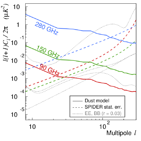
Figure 1.4: Estimated foreground levels for Spider. Over most of the angular scales of our observations, we expect to be dominated by dust foregrounds. Combining the maps made at both of our observing frequencies, as well as using data from Planck, will let us remove this contamination and after our second flight we will reach a final inflationary B-mode sensitivity of $r=0.03$ at $99\%$ confidence. Figure from Fraisse et al. [fraisse13].