RBC and UKQCD Collaborations

Edinburgh-2014/03

Hierarchically deflated conjugate gradient

Abstract

We present a multi-level algorithm for the solution of five dimensional chiral fermion formulations, including domain wall and Mobius Fermions. The algorithm operates on the red-black preconditioned Hermitian operator, and directly accelerates conjugate gradients on the normal equations. The coarse grid representation of this matrix is next-to-next-to-next-to-nearest neighbour and multiple algorithmic advances are introduced, which help minimise the overhead of the coarse grid. The treatment of the coarse grids is purely four dimensional, and the bulk of the coarse grid operations are nearest neighbour. The intrinsic cost of most of the coarse grid operations is therefore comparable to those for the Wilson case. We also document the implementation of this algorithm in the BAGEL/Bfm software package and report on the measured performance gains the algorithm brings to simulations at the physical point on IBM BlueGene/Q hardware.

I Introduction

The index theorem Atiyah ; Brown guarantees the existence of low modes of a Dirac operator in topologically non-trivial $SU(N)$ gauge configurations, protected from zero only by the light quark mass. This poses a problem for Krylov solution of the covariantly coupled Dirac equation since the condition number of the matrices involved must necessarily diverge as $\frac{1}{am_{ud}}$. This problem must arise for any lattice action that possesses the correct continuum limit, since the density of these modes must be universal near the continuum limit.

Krylov sparse matrix inversions of these Dirac operators approximate the inverse of the Dirac operator applied on the initial residual with a polynomial of the Dirac matrix. The coefficients are chosen to minimise the residual under some norm, the details depending on the Krylov algorithm. Worst case bounds on convergence rates for conjugate gradients (CG) Hestenes can be obtained using the Chebyshev minimax polynomials Saad ; the minimax error is dependent on the range over which the Chebyshev approximation must be accurate, and as a result the convergence rate is determined by the condition number $\kappa=\frac{\lambda_{\rm max}}{\lambda_{\rm min}}$ of the Dirac matrix, with the ratio $\sigma$ of successive residuals given by

$$\sigma=\frac{\sqrt{\kappa}-1}{\sqrt{\kappa}+1}.$$ (1)

This convergence factor becomes unity in the limit of large condition number, and convergence necessarily becomes slow. However, if we suppose there is a physical density of instantons and anti-instantons, and that we are near the continuum limit, one expects a set of detached set of low virtuality eigenvectors of topological origin that could be removed from the problem via deflation Morgan:2001qr ; Darnell:2003mi ; Darnell:2007dr ; Stathopoulos:2007zi . After deflation, the convergence rate is determined by the improved condition number corresponding to the rest of the spectrum. As the number of these topological modes is proportional to the volume, the cost of the deflation is $O(V^{2})$. Scaling to the large volume limit therefore imposes considerable cost.

Problematic volume scaling has, in other areas of computational science, been alleviated to $O(V\log V)$ using multi-level algorithms Brandt . Gauge freedom has until recently posed a barrier in Lattice theory: the process of blocking gauge dependent variables must be gauge covariant and hence discovered on each configuration, and it is only recently that two broadly similar approaches have been successfully developed.

LuscherLuscher:2007se introduced the key concepts of local coherence of low modes; the low modes bear substantial local similarity. He defined blocked variables in a gauge covariant way, using inverse iteration of the lattice Dirac operator to produce vectors with near vanishing covariant derivative so that they are rich in low modes. Similar ideas were independently introduced in the smoothed aggregation algebraic multigrid contextBrezina . The gauge symmetry in QCD is likely a worst case example of the case of non-smooth matrix coefficients considered in the algebraic multigrid case. Luscher’s idea of local coherence is similar to the “weak approximation” property, and a vector posessing near vanishing covariant derivative is termed “algebraically smooth”, with blocked variables being named aggregates. This multigrid work propagated directly into the programme carried out in the US by a group spanning both particle physicists and the mathematical community Brannick:2007ue ; Brannick:2007cc ; Clark:2008nh ; Babich:2009pc ; Babich:2010qb

Most successful applications of this class of techniques to lattice QCD have been based on solution of the non-Hermitian system for Wilson and clover Fermions Luscher:2007se ; Brannick:2007cc ; Babich:2010qb ; Osborn:2010mb ; Frommer:2012mv ; Frommer:2013fsa ; Frommer:2013kla .

The methods differ in whether and how the blocked representation of the Dirac operator is introduce as a preconditioner, whether more than two levels are included, and in the method used to discover the relevant subspace. Some earlier effort has been invested in unpreconditioned domain wall Fermions using the normal equationsCohen:2012sh .

The purpose of this paper is to develop a similar method applicable to domain wall Fermions and other forms of five dimensional Cayley form chiral Fermion Kaplan:1992bt ; Shamir:1993zy ; Furman:1994ky ; Narayanan:1993sk ; Narayanan:1993ss ; Narayanan:1994gw ; Neuberger:1997bg ; Neuberger:1997fp ; Borici:1999da ; Borici:1999zw ; Kikukawa:1999sy ; Brower:2004xi ; Edwards:2005an ; Brower:2012vk . This five dimensional approach is somewhat more challenging because the negative bulk Wilson mass shifts the spectrum of the 5d Wilson operator such that there are modes in all four quadrants of the complex plane. Spectra not contained within an open half plane are known to lead to difficulties for non-Hermitian Krylov methodstrefethen since we must make a polynomial approximation to $\frac{1}{z}$ that must cover a region of the complex plane that contains the pole. Domain wall Fermions indeed follow this folklore. In terms of practical algorithms, to the author’s knowledge, almost all algorithms for 5d Cayley chiral Fermions have made use of the normal equations with one exception.

Since one of the most effective Krylov solvers for DWF is CG applied to the normal equations for the red-black preconditioned operator, we aim to start from this most efficient point and in this paper develop and even faster algorithm based on inexact deflation. Since this operator is next-to-next-to-next-to-nearest neigbour the coarsened operator is considerably more non-local than for the Wilson operator and multiple algorithmic advances were required to obtain a real, measured speedup.

In section II we review the background of blocked deflation spaces that underlies both inexact deflation and adaptive multigrid. The algorithm we introduce will be hierarchical, however initially in section IV we shall consider only the two level approach and where one can initially assume for the sake of argument that all inner, coarse matrix inversions are performed exactly. Once the two level approach is established we will then consider in Section V introducing a second level when the application of the deflation matrix inverse, is performed in an inexact numerical implementation. We will study the performance of the algorithm in section VI.

II Blocked deflation subspace

In this section we introduce our notation for the building blocks of multi-level algorithms. To avoid critical slowing down in sparse matrix inversion, one can treat a vector subspace $S=\rm{span}\{\phi_{k}\}$ exactly. If the lowest lying eigenmodes are completely contained in $S$ the “rest” of the problem avoids critical slowing down. The method requires some setup since in a gauge theory this subspace is gauge dependent: one first must generate subspace vectors $\phi_{k}$ that are “rich” in low modes. We address in section IV.2 some procedures for how these vectors might be generated. Luscher observed that by subdividing these vectors into blocks $b$

$$\phi^{b}_{k}(x)=\left\{\begin{array}[]{ccc}\phi_{k}(x)&;&x\in b\\ 0&;&x\not\in b\end{array}\right.$$ (2)

we obtain a much larger subspace that, due to local coherence, is enormously more effective for deflation. These blocked vectors are locally orthogonalised using a Gramm Schmidt procedure. For example, on a $48^{3}\times 96$ lattice with $4^{4}$ blocks there is a $12^{3}\times 24$ coarse grid, and we obtain an $O(10^{4})$ bigger deflation space than one would expect from using the vectors $\phi_{k}$ without blocking. If the low modes are locally coherent, the span of block subvectors will better contain the low mode subspace than that of the global vectors because

$${\rm span}\{\phi_{k}\}\subset{\rm span}\{\phi_{k}^{b}\}.$$ (3)

We introduce blocked subspace projectors

$$P_{S}=\sum_{k,b}|\phi^{b}_{k}\rangle\langle\phi^{b}_{k}|\quad\quad;\quad\quad P_{\bar{S}}=1-P_{S}$$ (4)

and compute $M_{ss}$ as

$$M=\left(\begin{array}[]{cc}M_{\bar{S}\bar{S}}&M_{S\bar{S}}\\ M_{\bar{S}S}&M_{SS}\end{array}\right)=\left(\begin{array}[]{cc}P_{\bar{S}}MP_{\bar{S}}&P_{S}MP_{\bar{S}}\\ P_{\bar{S}}MP_{S}&P_{S}MP_{S}\end{array}\right)$$ (5)

We can represent the matrix $M$ exactly on this subspace by computing its matrix elements, known as the little Dirac operator (coarse grid matrix in multi-grid)

$$A^{ab}_{jk}=\langle\phi^{a}_{j}|M|\phi^{b}_{k}\rangle\quad\quad;\quad\quad(M_{SS})=A_{ij}^{ab}|\phi_{i}^{a}\rangle\langle\phi_{j}^{b}|.$$ (6)

the subspace inverse can be solved by Krylov methods and is:

$$Q=\left(\begin{array}[]{cc}0&0\\ 0&M_{SS}^{-1}\end{array}\right)\quad\quad;\quad\quad M_{SS}^{-1}=(A^{-1})^{ab}_{ij}|\phi^{a}_{i}\rangle\langle\phi^{b}_{j}|$$ (7)

It is important to note that $A$ inherits a sparse structure from $M$ because well separated blocks do not connect through $M$. We can Schur decompose the matrix

$$M=UDL=\left[\begin{array}[]{cc}M_{\bar{s}\bar{s}}&M_{\bar{s}s}\\ M_{s\bar{s}}&M_{ss}\end{array}\right] = \left[\begin{array}[]{cc}1&M_{\bar{s}s}M_{ss}^{-1}\\ 0&1\end{array}\right]\left[\begin{array}[]{cc}S&0\\ 0&M_{ss}\end{array}\right]\left[\begin{array}[]{cc}1&0\\ M_{ss}^{-1}M_{s\bar{s}}&1\end{array}\right]$$

Note that $P_{L}M=\left[\begin{array}[]{cc}S&0\\ 0&0\end{array}\right]$ yields the Schur complement $S=M_{\bar{s}\bar{s}}-M_{\bar{s}s}M^{-1}_{ss}M_{s\bar{s}}$, and that the diagonalisation $L$ and $U$ are related to Luscher’s projectors $P_{L}$ and $P_{R}$ (Galerkin oblique projectors in multi-grid)

$$P_{L}=P_{\bar{S}}U^{-1}=\left(\begin{array}[]{cc}1&-M_{\bar{S}S}M_{SS}^{-1}\\ 0&0\end{array}\right)\quad\quad;\quad\quad P_{R}=L^{-1}P_{\bar{S}}=\left(\begin{array}[]{cc}1&0\\ -M_{SS}^{-1}M_{S\bar{S}}&0\end{array}\right)$$ (9)

Finally, we require the relation $QM=1-P_{R}$. With a Hermitian system we gain the properties

$$P_{L}^{\dagger}=P_{R}\quad\quad\quad(P_{L}M)^{\dagger}=P_{L}M$$ (10)

II.1 Schur Complement Algorithms

Luscher introduced a class of algorithms based on the Schur decomposition. If we multiply the equation

$$M\psi=\eta$$ (11)

by $1-P_{L}$ and $P_{L}$ to obtain two equations yielding $(1-P_{R})\psi$ and $P_{R}\psi$, we have:

$$(1-P_{R})\psi = M_{ss}^{-1}\eta_{s}$$ (12)

$$(P_{L}M)\chi = P_{L}\eta$$ (13)

$$\psi = P_{R}\chi+M_{ss}^{-1}\eta_{s}$$ (14)

Solving Eq. 12 is easy, while for Eq 13 each step of an outer Krylov solver involves an inner Krylov solution of the little Dirac operator, entering entering the matrix $P_{L}M$ being inverted. Any errors in this little Dirac operator propagate into solution. Luscher alleviated this by tightening the precision during convergence, and using the history forgetting flexible GCR algorithm. The overhead of the little Dirac operator is suppressed by introducing the Schwarz alternating procedure (SAP) preconditioner as follows:

$$(P_{L}M)M_{SAP}\phi=P_{L}\eta\quad\quad;\quad\quad\psi=M_{SAP}\phi$$ (15)

In Luscher’s approach to Wilson fermions the little Dirac operator for $D_{W}$ is nearest neighbour, and although the fine operator does not make use of red-black preconditioning, red-black preconditioning of the little Dirac operator possible because the spatial structure is preserved in the coarse operator. This means that the Schwarz alternating procedure remains possible as $D_{W}$ does not connect red to red.

III Adaptive multigrid methods

Multigrid algorithms are typically expressed in a more heuristic manner than pure Krylov solvers. The underlying basic block is an error reduction step, taken with a (cheap) approximate inverse $\tilde{M}$:

$$r = \eta-M\psi$$ (16)

$$\psi^{\prime} = \psi+\tilde{M}r$$ (17)

$$\Rightarrow r^{\prime} = (1-M\tilde{M})r$$ (18)

To the extent that $\tilde{M}$ is a good approximate inverse a convergent process can be built from these steps. The adaptive multigrid Brannick:2007ue ; Brannick:2007cc ; Clark:2008nh ; Babich:2009pc ; Babich:2010qb ; Osborn:2010mb ; Frommer:2012mv ; Frommer:2013fsa ; Frommer:2013kla for QCD is well developed for Wilson and clover Fermions. They typically combine an inner V-cycle or W-cycle spanning representations of the Dirac matrix on multiple grids as a preconditioner to an outer Krylov solver, and since non-Hermitian systems are treated this is typically flexible GCR solver. As with Luscher’s algorithm they typically adopt the SAP procedure as a preconditioner, but this is organised as an error reducing smoother entering as one component in a sequence of error reduction steps on a multigrid cycle. The inclusion of these steps as a variable preconditioner is important since this allows composition when each each step is an aggressively truncated Krylov process bearing substantial variability. For Hermitian (symmetric) matrices a symmetric V-cycle is required for conjugate gradients, consisting of both pre- and post-smoothing steps to ensure Hermiticity. In later sections we will see how this can be avoided.

IV Generalisation to 5d Chiral Fermions

To generalise Luscher’s approach, we must implement a method suitable for Krylov solution of the Hermitian system. In this work we will aim to speed up solution for the red-black preconditioned system, as this starting point is the best presently known approach and so any speed up over the baseline is a genuine gain. We define the Hermitian red-black operator ${\cal H}$ as:

$${\cal H}=\left(M_{oo}-M_{oe}M_{ee}^{-1}M_{eo}\right)^{\dagger}\left(M_{oo}-M_{oe}M_{ee}^{-1}M_{eo}\right)=M_{\rm prec}^{\dagger}M_{\rm prec}$$ (19)

The Hermitian naure of this matrix is an advantage for subspace generation, which we discuss below. There are also several significant challenges that arise because the operator is is next-to-next-to-next-to-nearest-neighbour in four dimensions, and entirely non-local in the fifth dimension. Firstly we address the non-locality as follows. We do not block the fifth dimension to address the non-locality. In four dimensions the matrix stencil still connects 320 neighbours compared to the eight for the Wilson non-Hermitian system; a substantial suppression of the little Dirac operator overhead must be found to alleviate this additional cost. Secondly, since the matrix is not nearest neighbour the alternating procedure cannot be applied; we require an alternative to the Schwarz preconditioner. Thirdly, we must find an appropriate solver: $(P_{L}M)M_{SAP}$ is a non-Hermitian matrix so is unsuitable for Hermitian solver algorithms such as conjugate gradients. Finally we must ensure the system is tolerant to loose convergance of the inner Krylov solver(s); this is needed to relax the stopping conditions, similar to the flexibility introduced in Luscher’s algorithm. We address these issues in turn.

IV.1 Preconditioned conjugate gradient for Schur complement

1. $r_{0}=b-Ax_{0}$ 2. $z_{0}=M_{IRS}r_{0}$ ; $p_{0}=z_{0}$ 3. for iteration $k$ 4. $\alpha_{k}=(r_{k},z_{k})/(p_{k},Ap_{k})$ 5. $x_{k+1}=x_{k}+\alpha_{k}p_{k}$ 6. $r_{k+1}=r_{k}-\alpha_{k}Ap_{k}$ 7. $\mathbf{z_{k+1}=M_{IRS}r_{k+1}}$ 8. $\mathbf{\beta_{k}=(r_{k+1},z_{k+1})/(r_{k},z_{k})}$ 9. $\mathbf{p_{k+1}=z_{k+1}+\beta_{k}p_{k}}$ 10. end for

Figure 1: Preconditioned conjugate gradient algorithm. In the iteration both $M_{IRS}$ and $A=P_{L}M$ contain inner Krylov solves. However $M_{IRS}$ only enters the selection of the search direction $p_{k}$, while the little Dirac inversion directly enters the linear combination coefficient $\alpha_{k}$. We observe a drastically different sensitivity to the precision of the two inner inversions.

We initially applied the standard preconditioned CG AxelssonPcg ; p278Saad given in figure 1 to the Schur complement operator

$$P_{L}{\cal H}=\left(\begin{array}[]{cc}1&-M_{\bar{S}S}M_{SS}^{-1}\\ 0&0\end{array}\right){\cal H}.$$ (20)

Each iteration used two inner Krylov solvers: the little Dirac operator inversion

$$Q\equiv M_{SS}^{-1}$$ (21)

entering $P_{L}$, and the IR shifted preconditioner inversion

$$M_{IRS}=\frac{1}{{\cal H}+\lambda}.$$ (22)

The convergence precision on both of these is independently controllable and we will shortly study the sensitivity of the overall convergence to both these Krylov inversions independently. Although this is not the final manifestation of the new algorithm, the initial simplicity of preconditioned CG is helpful for framing the following discussion. This is particularly the case since the structure is very similar to that of Luscher’s algorithmLuscher:2007se .

IV.2 Subspace generation

Since we are dealing with a Hermitian positive definite operator, an efficient subspace generation can be performed using a multi-shift solver to approximate a fourth order rational low-pass filter applied to Gaussian noise vectors $\eta_{k}$, without the need for inverse iteration.

$$\phi_{k}=R(\eta_{k})\propto\frac{1}{({\cal H}+\lambda)({\cal H}+\lambda+\epsilon)({\cal H}+\lambda+2\epsilon)({\cal H}+\lambda+3\epsilon)}$$ (23)

Typically we take $\lambda=0.0003$ and $\epsilon=\lambda/3$, however this depends on the normalisation and condition number of the operator. The response function of this rational filter is illustrated in figure 2. As one expects for domain wall Fermions the resulting vectors have non-trivial structure in the fifth dimension being largely bound to the walls. This statement remains true for the preconditioned Hermitian Mobius Fermion case, figure 3.

This profile may be exploited in several ways. A modest improvement in the quality of subspace was obtained by generating four dimensional Gaussian noise vectors $\eta_{k}$ and placing this only on the physical field components of the walls as the input to our rational filter, thus better matching the input vector to these physical modes and requiring less effort to be applied in the filtering.

Two efficient strategies have been found, and which is more efficient depends on $L_{s}$. Firstly solving $R(\eta_{k})$ to $10^{-6}$ is efficient for modest $L_{s}$. Secondly, we can generate the subspace vectors in two stages: a first pass approximation is generated by solving $R(\eta_{k})$ with reduced precision and reduced $L_{s}$ ranging between eight and twelve. These are promoted to the surface regions of the full system, a second pass uses the first pass deflated solver to improve the subspace filling in the fifth dimension bulk. This second pass applies a single shifted inversion $[{\cal H}+\lambda]^{-1}$ to the first pass subspace vectors (after promotion to the increased $L_{s}$) to some precision.

The code implementation can also optionally remove the interior of a subset of the subspace vectors, recognising that they are near zero in this region. This limits the growth of the cost of subspace generation, and of projection to and from the coarsened problem with $L_{s}$, while the coarse problem cost does not depend on $L_{s}$.

BAGEL and the associate BFM (Bagel Fermion Matrix) package have an implementation of HDCG Boyle:2009bagel . The parameters in the BFM implementation of HDCG controlling subspace generation are tabulated in Table 1.

Parameter	Meaning
SubspaceRationalLo	Low pass filter threshold $\lambda$
SubspaceRationalLs	Extent of fifth dimension used in first pass subspace
SubspaceRationalResidual	Multishift solver convergence residual for first pass subspace
SubspaceRationalRefine	Whether to generate a second pass subspace
SubspaceRationalRefineResidual	Singleshift solver residual for second pass subspace
SubspaceRationalRefineLo	Low pass filter threshold $\lambda$ for second pass subspace
SubspaceSurfaceDepth	The depth in s-slices neighbouring the surface preserved in subspace vectors

Table 1: Parameters to HDCG for controlling the generation of the fine grid deflation space. If a second pass is used the deflated solver generated by the first pass subspace is used to accelerate the generation of the second pass subspace. The second pass refinement consists of a single shift inversion with the full five dimensional system.

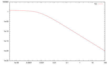
Figure 2: A single multishift inversion can well approximate a 4th order rational low pass filter and be used in low mode subspace generation. The bandpass parameter $\lambda$ protects the condition number of the inversions, while only a single pass is required. Together these make the process relatively cheap compared to inverse iteration. The filter function is given in Eq. 23, and we display the exact result obtained if the multishift inversion was applied to very high convergence precision.

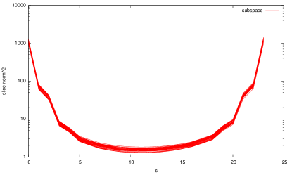
Figure 3: Dependence of the norm of four dimensional slices of the subspace vectors on the coordinate in the fifth dimension. Even for the preconditioned Hermitian Mobius Fermion case the lowest modes are bound to the walls. All vectors obtained on a single configuration are overlayed, and the shape profile is non-trivial. This shape profile can be used to our advantage in several ways (both in subspace generation and accelerating the projection/promotion from the coarse spaces) since the interior segments become negligible for large $L_{s}$.

IV.3 Infra-red shift preconditioner $M_{IRS}$

We aim to use outer iterations based on preconditioned CG (in a more modern form) AxelssonPcg ; p278Saad with a Hermitian preconditioner. A high mode preconditioner is required to limit the cost overhead associated with the little Dirac operator.

In the multigrid literature this preconditioner would be called a smoother, while in Luscher’s algorithm some fixed number of iterations of the Schwarz alternating procedure is used. Since we are deflating the low modes, we seek approximate inverse preconditioner for the Hermitian system that is both Hermitian positive definite and is a cost effective approximate inverse reasonably accurate for high modes.

BFM supports a number of options relating to the preconditioner for the outer Krylov process, listed in table 2.

Option	Value	meaning
PreconditionerType	Mirs	Fixed number of CG iterations with a infrared shift
	MirsPoly	Fixed polynomial. Coefficients determined by one pass of CG
	Chebyshev	Chebyshev polynomial preconditioner
	None	No fine grid preconditioner
PreconditionerKrylovIterMax	int	Preconditioner iterations (or chebyshev order)
PreconditionerKrylovLo	double	Lowest eigenvalue targeted by preconditioner
PreconditionerKrylovHi	double	Upper limit of eigenrange for Chebyshev preconditioner

Table 2: Options controlling outer Krylov preconditioner for HDCG implementation. PreconditionerType must be set to one of PreconditionerMirs, PreconditionerMirsPoly, PreconditionerChebyshev, or PreconditionerNone. PreconditionerKrylovIterMax controls either the order of a polynomial or the number of Krylov iterations as appropriate. PreconditionerKrylovLo controls the eigenrange for both Krylov based preconditioners and for the Chebyshev polynomial based preconditioner, while PreconditionerKrylovHi applies only to the Chebyshev preconditioner. In practice we find that PreconditionerMirs is the best option on physical point configurations.

The $M_{IRS}$ preconditioner is based on a fixed number of shifted CG iterations acting with a shifted matrix, and applied in single precision,

$$M_{IRS}({\cal H},N_{CG},\lambda)=\left.\frac{1}{{\cal H}+\lambda}\right|_{N_{CG}\rm iterations}.$$ (24)

Here, $\lambda$ is a gauge covariant infra-red regulator that plays a similar role to the domain size in SAP. Since a Krylov solver minimises the error of a polynomial under some norm, the infra-red shift (IRS) ensures the turning points of the error polynomial lie in the high eigenvalue region we wish to improve with the preconditioner. This ensures that the two preconditioners remain complementary.

A typical polynomial produced by the $M_{IRS}$ conjugate gradient may be seen in figure 4. The lower range of the region of accuracy is set by the infra-red regulator $\lambda$. The upper range is selected by the optimality of conjugate gradient, and thus detected by the algorithm based on the spectrum of the operator and the spectral content of the initial residual. In the example shown, the unpreconditioned operator has upper edge of its spectrum at around $\lambda\sim 90.0$, while this should lowered to around $\lambda\sim 1.0$ by the $M_{IRS}$ preconditioner with convergence rate correspondingly improved by the reduced condition number of the preconditioned operator.

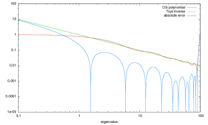
Figure 4: Conjugate gradient approximate inverse polynomial selected by nine iterations of conjugate gradient applied in $M_{IRS}$ with a low pass parameter $\lambda=1.0$. Compared to the CG based polynomial preconditioner of Oleary the inclusion of the infra-red shift has a stabilising effect. The automatic selection of the upper edge of the spectrum (at around eigenvalue $\lambda\sim 90$) is an advantage compared to Chebyshev preconditioners since the number of tunable parameters is reduced. In fact, it turns out that the dynamic response of CG to the spectral content of the residual is important; running a fresh Krylov process for each preconditioner application (PreconditionerMirs) results in faster convergence than freezing this with a static polynomial (PreconditionerMirsPoly).

IV.3.1 Alternative polynomial preconditioners

Reusing the polynomial created by CG from a fixed number of iterations as a preconditioner has been previously studied Oleary . In that study the problem arose that this polynomial, although Hermitian, may not be positive definite and damage the outer convergence. The infra-red shift, as far as the author is aware first introduced in our work, greatly stabilises the CG polynomial and can be used to keep the polynomial sign definite over the range $[0,\infty)$ for even order polynomials. By keeping the preconditioner a data dependent Krylov process, optimal under some norm, we appear to gain in stability. Replaying the CG polynomial eliminates a single matrix multiply, and also eliminates linear algebra in each iteration gaining around 10% in runtime. On the other hand, it turns out that the dynamic response of CG to the spectral content of the residual is also important at the 10%; running a fresh Krylov process for each preconditioner application (PreconditionerMirs) results in faster convergence than freezing this with a static polynomial (PreconditionerMirsPoly) and these are roughly competitive with each other.

We also compared to Chebyshev preconditioning. For the $M_{IRS}$ preconditioner the tuning problem is vastly reduced since the upper end of the spectrum need not be identified. The Chebyshev preconditioner is particularly sensitive to the high parameter since the polynomial explodes rapidly above this threshold, while the optimal upper edge is found automatically by a CG based process. However, when well tuned the Chebyshev preconditioner can also almost as effective.

The two IRS preconditioners $M_{IRS}$ and $M_{IRSpoly}$ introduced in this paper are, as far as the author is aware, wholly new components of the algorithm.

IV.4 Robustness and flexibility

We observe curious robustness effects during solution to $10^{-8}$ on a $16^{3}$ lattice in table 3. The preconditioned CG inverting the Schur complement operator $P_{L}{\cal H}$ is almost completely insensitive to the precision of the preconditioner $M_{IRS}$ but is highly sensitive to errors in the little Dirac operator inversion $Q=M_{SS}^{-1}$. Indeed convergence beyond the precision to which $Q$ is evaluated is not possible.

$M_{SS}^{-1}$ residual	$M_{IRS}$ residual	Iteration count
$10^{-11}$	$10^{-8}$	36
$10^{-8}$	$10^{-8}$	Non converge
$10^{-11}$	$10^{-8}$	36
$10^{-11}$	$10^{-4}$	36
$10^{-11}$	$10^{-2}$	36

Table 3: Sensitivity of the Schur complement inversion (DEF1) to both little Dirac operator residual, and to the preconditioner residual. This corresponds to Luscher’s algorithm, and it appears that preconditioned CG is remarkably insensitive to preconditioner variability.

This confirms results in the numerical literature GolubYe . Although flexible CG existsNotay and could be used to enhance tolerance to variability, we observe that CG is already surprisingly tolerant to variability in $M_{IRS}$ but not $Q$. This may be understood as follows: in PCG, the noise in the preconditioner $M_{IRS}$ only enters the search direction, while the linear combination coefficients entering the solution and residual update are based on matrix elements of $P_{L}{\cal H}$. In particular the multigrid papers also use the coarse grid operator as a preconditioner and are less sensitive to convergence noise; it is this that admits the composition of many imprecise levels in a multi-grid cycle scheme. One can certainly conclude that it is better to use the little Dirac operator inverse as a preconditioner and not separate the solution into subspace and complement.

IV.5 Improved solver framework

To move the little Dirac operator into the preconditioner we extend framework of Tang to three levels as follows. First we consider the most general possibilities for combining in a single preconditioner a little Dirac operator $Q$ and $M_{IRS}$, each representing approximate inverses, where $Q$ operates on a subspace containing almost all low modes and overlapping with a subset of high modes (the splitting is necessarily inexact due to the theta function that restricts vectors to blocks), and $M_{IRS}$ is accurate on the high mode space. Among the options for combining these as a preconditioner in an outer solver is the naive additive case: $M_{IRS}+Q$. However, we can also consider alternating error reduction steps, such as:

$$\begin{array}[]{ccc}x_{i+1}&=&x_{i}+M_{IRS}[b-{\cal H}x_{i}]\\ x_{i+2}&=&x_{i+1}+Q[b-{\cal H}x_{i+1}]\\ &=&x_{i}+M_{IRS}[b-{\cal H}x_{i}]+Q[b-{\cal H}[x_{i}+M_{IRS}[b-{\cal H}x_{i}]]]\\ &=&x_{i}+[(1-Q{\cal H})M_{IRS}+Q](b-{\cal H}x_{i})\\ &=&x_{i}+[P_{R}M_{IRS}+Q](b-{\cal H}x_{i})\end{array}$$ (25)

We can similarly infer the family of preconditioners listed in table 4 by choosing different sequences of error reduction steps.

Sequence	Preconditioner	Name
additive	$M_{IRS}+Q$	AD
$M_{IRS}$, $Q$	$P_{R}M_{IRS}+Q$	A-DEF2
$Q$, $M_{IRS}$	$M_{IRS}P_{L}+Q$	A-DEF1
$Q$, $M_{IRS}$, $Q$	$P_{R}M_{IRS}P_{L}+Q$	Balancing Neumann Neumann (BNN)
$M_{IRS}$, $Q$, $M_{IRS}$	$M_{IRS}P_{L}+P_{R}M_{IRS}+Q-M_{IRS}P_{L}{\cal H}M_{IRS}$	MG Hermitian V(1,1) cycle

Table 4: In fact, a whole family of preconditioners arrived at by composing the little Dirac operator and the IRS preconditioner. The IRS preconditioner can thought of as a smoother in the multigrid context. For a HPD outer solver algorithm, multigrid requires to use the V(1,1) cycle in the final row to preserve Hermiticity.

We take $Q=\left(\begin{array}[]{cc}0&0\\ 0&M_{SS}^{-1}\end{array}\right)$ and $M_{IRS}=({\cal H}+\lambda)^{-1}$ (or substitute $M_{IRSpoly}$ as appropriate), and implemented the generalised preconditioned conjugate gradient algorithm in figure 5 and with the complete set of preconditioning options documented in table 5. Of these, we find that A-DEF2 is the most numerically efficient because the little Dirac operator inverse enters only once, and in the preconditioning step so that the solution can be made very approximate (see previous section). The matrices in A-DEF1 and A-DEF2 are not manifestly Hermitian and further work is needed to show that one can expect convergence of an outer conjugate gradient. In fact it turns out that DEF1(Luscher), DEF2, A-DEF1, A-DEF2, and BNN are equivalent up to the convergence precision of the little Dirac operator for appropriate start vectors. Thus the convergence rates only differ in thier sensitivity to imprecision in inner Krylov inversions. We may see this as follows.

1. $x$ arbitrary 2. $x_{0}=V_{\rm start}$ 3. $r_{0}=b-{\cal H}x_{0}$ 4. $y_{0}=M_{1}r_{0}$ ; $p_{0}=M_{2}y_{0}$ 5. for iteration $k$ 6. $w_{k}=M_{3}{\cal H}p_{k}$ 7. $\alpha_{k}=(r_{k},y_{k})/(p_{k},w_{k})$ 8. $x_{k+1}=x_{k}+\alpha_{k}p_{k}$ 9. $r_{k+1}=r_{k}-\alpha_{k}w_{k}$ 10. $\mathbf{y_{k}=M_{1}r_{k}}$ 11. $\mathbf{\beta_{k}=(r_{k+1},y_{k+1})/(r_{k},y_{k})}$ 12. $\mathbf{p_{k+1}=M_{2}y_{k+1}+\beta_{k}p_{k}}$ 13. end for 14. $x=V_{\rm end}$

Figure 5: Generalised preconditioned conjugate gradient algorithm of Tang et alTang . The choice of matrices $M_{1}$, $M_{2}$, $M_{3}$ and vectors $V_{\rm start}$ and $V_{\rm end}$ interpolate between Hermitian $V(1,1)$ multigrid, Luscher’s Schur complement method, and introduce several new approaches. Of these this paper focuses on the A-DEF2 method which minimises little Dirac operator overhead while keeping all inner Krylov solves in the preconditioner, and proves to be the most robust. We have also implemented “inexact preconditioned CG”GolubYe and “flexible CG” Notay variants of this algorithm and these generalisations are simple to implement and as a result are not documented in this paper to avoid repetitition.

Method	$V_{\rm start}$	$M_{1}$	$M_{2}$	$M_{3}$	$V_{\rm end}$
PREC	$x$	$M_{IRS}$	$1$	$1$	$x_{k+1}$
AD	$x$	$M_{IRS}+Q$	$1$	$1$	$x_{k+1}$
DEF1	$x$	$M_{IRS}$	$1$	$P_{L}$	$Qb+P_{R}x_{k+1}$
DEF2	$Qb+P_{R}x$	$M_{IRS}$	$P_{R}$	$1$	$x_{k+1}$
A-DEF1	$x$	$M_{IRS}P_{L}+Q$	$P_{R}$	$1$	$x_{k+1}$
A-DEF2	$Qb+P_{R}x$	$P_{R}M_{IRS}+Q$	$1$	$1$	$x_{k+1}$
BNN	$x$	$P_{R}M_{IRS}P_{L}+Q$	$1$	$1$	$x_{k+1}$
Multigrid	$x$	$M_{IRS}P_{L}+P_{R}M_{IRS}+Q-M_{IRS}P_{L}{\cal H}M_{IRS}$	$1$	$1$	$x_{k+1}$

Table 5: Spectrum of possible choices for the generalised algorithm. DEF1 generates a Schur complement inverter similar to Luscher’s original algorithm, while mutilgrid corresponds to the standard symmetric V(1,1) cycle. The matrices in A-DEF1 and A-DEF2 are not manifestly Hermitian and further work is needed before once can expect convergence of an outer conjugate gradient. If we use $M_{IRSpoly}$ then PREC is a polynomial preconditioned conjugate gradient with zero setup cost. We find the best algorithm is A-DEF2.

IV.5.1 Hermiticity proof for A-DEF2

The Hermiticity of $M_{1}$ is clear for BNN but not A-DEF2. However, we will reproduceTang a proof that for $V_{\rm start}=Qb+P_{R}x$ A-DEF2 is identical to BNN.

We have from $Q{\cal H}=(1-P_{R})$,

$$Qr_{0}=Q[{\cal H}V_{\rm start}-b]=(1-P_{R})[Q_{b}+P_{R}x]-Qb=P_{R}Q_{b}=0,$$ (26)

and

$$Q{\cal H}p_{0}=(1-P_{R})[P_{R}MP_{L}+Q]r_{0}=0.$$ (27)

We obtain induction steps:

$$Qr_{j+1}=Qr_{j}-\alpha_{j}Q{\cal H}p_{j}=0,$$ (28)

$$Q{\cal H}p_{j+1}=(1-P_{R})[P_{R}MP_{L}+Q]r_{j}+\beta_{j}Q{\cal H}p_{j}=0.$$ (29)

We can similarly show $P_{L}r_{0}=0$ and $P_{L}{\cal H}p_{0}={\cal H}p_{0}$ so that

$$P_{L}{\cal H}p_{j+1}={\cal H}P_{R}[P_{R}MP_{L}+Q]r_{j}+\beta_{j}p_{j}={\cal H}p_{j+1},$$ (30)

and

$$P_{L}r_{j+1}=P_{L}r_{j}-\alpha_{j}P_{L}{\cal H}p_{j}=r_{j}-\alpha_{j}{\cal H}p_{j}=r_{j+1}.$$ (31)

The consequence is that BNN then retains $P_{L}r_{j}=r_{j}$ in exact evaluation, and the BNN preconditioning ($P_{R}MP_{L}r_{j}$) and A-DEF2 preconditioning ($P_{R}Mr_{j}$) must remain equivalent up to convergence error of the inner Krylov steps. In fact ref Tang shows that DEF1(Luscher), DEF2, A-DEF1, A-DEF2, BNN are all equivalent up to convergence, but they differ hugely in the sensitivity to this convergence precision.

It is interesting to note that since the equivalence of ADEF-2 iterates to those of a Hermitian preconditioner is inductive, it is a proof that can only be obtained in a Krylov approach where the outer iteration steps are known. In this sense the reduction of the number of smoothing steps from two in the case of the Hermitian V(1,1) multigrid cycle to one in the case of ADEF-2 does not appear to be a step one can take in the conventional multi-grid approach.

IV.5.2 Bfm solver algorithm support

The BFM implementation supports many configurable solver options for the outer solver, documented in table 6, for the outer level Krylov solver. The outer solver search direction update may be varied to implement the standard, inexact preconditioned, and flexible variants of preconditioned conjugate gradients. The PcgType controls which of the two level algorithms introduced byTang are implemented.

This completes the discussion of the finest grid, and in the following section we now consider the optimised implementation of the second level as an inexact Krylov process.

Preconditioner controls
Parameter	Value	Meaning
PcgType	PcgPrec	Single grid – only use $M_{IRS}$ preconditioning
	PcgAD	Additive preconditioning algorithm
	PcgDef1	Def1 preconditioning algorithm
	PcgDef2	Def2 preconditioning algorithm
	PcgADef1	Adapted Def2 preconditioning algorithm
	PcgAdef2	Adepted Def1 preconditioning algorithm
	PcgBNN	Balancinng Neumann-Neumann preconditioner
	PcgMssDef	Use only the little Dirac operator as preconditioner (no smoother)
	PcgAdef2f	Adapted Def2 using single precision preconditioner
	PcgV11f	Hermitian V11 cycle multigrid using single precision preconditioner
Search direction controls
Outer Solver	Pcg	Preconditioned CG
	iPcg	Inexact preconditioned CG
	fPcg	Flexible preconditioned CG

Table 6: Options controlling behaviour of BFM HDCG outer solver. The recommended algorithm is PcgAdef2f combined with Flexible CG which makes use of single precision acceleration and has robust convergence.

V Little Dirac operator treatment

In this section we report on three techniques used to alleviate the cost of the little Dirac operator, and on several implementation issues.

V.1 Reducing coarse operator overhead

In our approach we limit the stencil of the Little Dirac operator by requiring each block dimension be $\geq 4^{4}$. Since for Mobius Fermions $M_{ee}^{-1}$ is entirely non-local in $s$-direction, we let the blocks stretch the full extent of the s-direction. These constraints leave the little Dirac operator as a sparse in 4d with next-to-next-to-next-to-nearest coupling, but which takes no more than one hop in each direction. For such blockings the coarse matrix only connects to 80 neighbours:

($\pm\hat{x}$), ($\pm\hat{y}$), ($\pm\hat{z}$), ($\pm\hat{t}$)

( $\pm\hat{x}\pm\hat{y}$), ( $\pm\hat{x}\pm\hat{z}$), ($\pm\hat{x}\pm\hat{t}$) , ($\pm\hat{y}\pm\hat{z}$), ( $\pm\hat{y}\pm\hat{t}$), ( $\pm\hat{z}\pm\hat{t}$)

( $\pm\hat{x}\pm\hat{y}\pm\hat{z}$), ( $\pm\hat{x}\pm\hat{y}\pm\hat{t}$), ( $\pm\hat{x}\pm\hat{z}\pm\hat{t}$), ( $\pm\hat{y}\pm\hat{z}\pm\hat{t}$)

( $\pm\hat{x}\pm\hat{y}\pm\hat{z}\pm\hat{t}$)

The underlying cost is reduced to only ten times more than non-Hermitian system, however, reducing to 4d has potentially saved an $L_{s}$ factor. The saving is overestimated as we likely require more vectors to describe 5th dimension. In our implementation of the little Dirac operator for BlueGene/Q haring2012ibm ; Boyle:2012iy good efficiency was required since the BAGEL/Bfm implementationBoyle:2009bagel of the fine operator performs around 10x that of compiled code. Fortunately, dense matrix-vector operations were amenable to optimisation using vector intrinsics for the IBM xlc compiler achieving over $60$ Gflop/s in single precision. The communication latency associated with the 80 small messages was reduced by around fifty fold using the SPI communications layer, and offloading the eighty packets to DMA can be performed in under ten microseconds.

The little Dirac operator inherits Hermiticity and sparsity from the fine Hermitian matrix. The inverse of the little Dirac operator is applied by Krylov methods. Conjugate gradient, deflated conjugate gradient, ADEF1, ADEF2, and multi-shift conjugate gradient methods were implemented.

V.1.1 Calculation of little Dirac operator matrix elements

The non-local stencil makes it somewhat harder to determine the matrix elements

$$A^{ab}_{jk}=\langle\phi^{a}_{j}|{\cal H}|\phi^{b}_{k}\rangle.$$ (32)

In the nearest neighbour coupled non-Hermitian and unpreconditioned case it is cheap to determine all non-zero matrix elements. In our non-Hermitian case the matrix elements between each blocked vector and the 80 nearby blocks may always be computed with only 81 matrix multiplies using a Fourier trick as follows. Other schemes are possible, such as coloring schemes, but this trick simplifies programming when the stencil size of the coarse operator (3) does not divide the global coarse lattice size.

We create 81 complex phases $z^{s}_{b}$ for each block $b$ and indexed by $s$. These are

$$z^{s}_{b}=e^{ip^{s}_{\mu}x_{\mu}^{b}}$$ (33)

where the block $b$ has block coordinates $x_{\mu}^{b}$ in the coarse grid. These phases correspond to low lying Fourier modes $p^{s}_{\mu}=n^{s}_{\mu}\frac{\pi}{L_{\mu}}$ on the coarse grid with up to one unit of momentum in each direction. Hence $s$ indexes the $81=3^{4}$ neighbours of zero in momentum space and this has the same dimension as the coarse grid stencil. For each $s$ and $\mu$, $n^{s}_{\mu}\in\{-1,0,1\}$. For each subspace vector $\phi_{k}$ and Fourier mode $s$, we compute vectors containing these phases multiplying each sub-block

$$|\tilde{\phi}_{k}(p^{s})\rangle=\sum_{b}e^{ip^{s}_{\mu}x^{b}_{\mu}}|\phi^{b}_{k}\rangle.$$ (34)

We apply the Hermitian matrix and construct matrix elements for each Fourier mode $p^{s}$ as follows

$$e^{-ip^{s}_{\mu}x^{b}_{\mu}}\langle\phi_{k^{\prime}}^{b}|{\cal H}|\tilde{\phi}_{k}(p^{s})\rangle=\sum_{l\in{\rm stencil}}e^{ip^{s}_{\mu}\delta^{l}_{\mu}}\langle\phi_{k}^{b}|{\cal H}|\phi^{b+l}_{k}\rangle=\sum_{l\in{\rm stencil}}M_{sl}\langle\phi_{k}^{b}|{\cal H}|\phi^{b+l}_{k}\rangle,$$ (35)

where $\delta^{l}_{\mu}$ is the coordinate space translation, in coarse grid coordinates, associated with element $l$ of the stencil. Having assembled the matrix elements of the 81 Fourier modes we can invert the matrix

$$M_{sl}=e^{ip^{s}_{\mu}\delta^{l}_{\mu}}$$ (36)

and form the matrix elements as

$$\langle\phi_{k}^{b}|{\cal H}|\phi^{b+l}_{k}\rangle=M^{-1}_{ls}e^{-ip^{s}_{\mu}x^{b}_{\mu}}\langle\phi_{k^{\prime}}^{b}|{\cal H}|\tilde{\phi}_{k}(p^{s})\rangle$$ (37)

This inversion can be performed sequentially in the four dimensions, similar to a multi-dimensional Fourier transform.

V.2 Little Dirac operator solver

The BFM implementation supports many configurable solver options, documented for the inner level Krylov solver in table 7.

Parameter	Value	Meaning
LittleDopSolver	LittleDopSolverMCR	Modified conjugate residual
	LittleDopSolverCG	Conjugate gradient
	LittleDopSolverDeflCG	Deflated conjugate gradient
	LittleDopSolverADef2	A-Def2 algorithm
	LittleDopSolverADef1	A-Def1 algorithm

Table 7: Options controlling the BFM HDCG inner solver algorithm. The recommended algorithm is LittleDopSolverAdef1 which uses the truncation of the little Dirac operator to nearest neighbour as a smoother in combination with a second level deflation space.

V.2.1 Little Dirac operator deflation

We then obtain a further speed up by deflating the deflation matrix, making the algorithm hierarchical. We compute the second level of global vectors (with no further blocking) in the deflation hierarchy using either three steps of inverse iteration with a shifted matrix, or the 4th order rational filtering technique. We produce around 128 deflation vectors in addition to the original fine grid subspace vectors. We again find that multi-shift inversion is more cost effective.

These vectors are used to augment the set of easily obtained global deflation vectors discussed in appendix A.3 of Luscher:2007se .

Although three levels are involved, the coarsest level is a single dense matrix. We diagonalise this basis to make by multiplication the third level operator cheap. This pattern of grid structures is identical to that used in Luscher’s original algorithm Luscher:2007se , but we augment the second deflation subspace beyond those vectors that are free to obtain.

The parameters in the BFM implementation used to control the generation Table 8.

Parameter	Meaning
LittleDopSolverResidualSubspace	Residual to use during subspace generation
LittleDopSubspaceRational	Whether to use rational filtering (true) or inverse iteration (false)

Table 8: Parameters to HDCG for controlling the generation of the coarse grid deflation space. The same low pass filter threshold is used for the little Dirac operator as for the fine dirac operator.

When we combine this deflation speed up with a relaxed convergence criterion discussed in section IV.5 we find around a 100 fold reduction in little Dirac operator overhead on $48^{3}$ simulations at physical quark masses, table 9.

Precision	Hierarchical deflation	iterations
$10^{-7}$	N	4478
$10^{-7}$	Y	250
$10^{-2}$	Y	63

Table 9: Reduction in little Dirac operator overhead enabled by a second level of deflation and by a reduction in required precision that comes from using the little Dirac operator in a preconditioner.

V.2.2 Truncated little Dirac operator as preconditioner

We can also use the improved solver framework to accelerate the inversion of the little Dirac operator $Q$ beyond simple deflated CG. In particular, we may introduce a cheap approximate inverse matrix acting on high modes of the little Dirac operator to augment the global vector deflation as follows.

Hops	Frobenius norm	number terms
0	627	1
1	6.2	9
2	0.08	33
3	0.0007	65
4	0.00003	81

Table 10: We display the Frobenius norm of the $N_{\rm vec}\times N_{\rm vec}$ matrix $A_{jk}^{bb^{\prime}}$ connecting two blocks $b$ and $b^{\prime}$ separated by a distance of taxicab norm measured as a number of hops. The matrices clearly fall rapidly with distance, while the number of such matrices grows less rapidly.

The cost associated with the next-to-next-to-next-to-nearest neighbour Little Dirac operator stencil may be alleviated considerably. The coefficients of the matrix fall rapidly with distance, table 10, and this may be exploited by truncating the matrix to finite range and using this in a preconditioner. Table 10 shows that omitting these terms is a small perturbation to the Little Dirac operator and we produce a range truncated matrix $Q_{\rm trunc}$ which includes only the zero and one hop terms, but remains Hermitian.

When used as the preconditioner in our second level of deflation $Q_{\rm trunc}$ is appealing because the cost of the truncated nearest neighbour preconditioner is nine times less than the cost of the the unmodified next-to-next-to-next-to-nearest neighbour little Dirac operator $Q$.

However, perturbing the smallest eigenvalues of the matrix $Q$ in an uncontrolled way is not necessarily wise since it could make the truncated matrix less well conditioned or even sign indefinite. This problem can however be avoided because by applying a modest infrared shift we preserve positivity of the eigenvalues, and protect the condition number.

We can therefore construct high mode preconditioners for the little Dirac operator, and use these in combination the second level of low mode deflation previously discussed. We do this by using the ADEF1 algorithm as the for solver the little Dirac operator. Both the subspace vectors for the little Dirac operator $\phi_{k}$ and the vectors $A\phi_{k}$ can be stored, and since no further blocking is performed the ADEF1 algorithm is preferable because by precomputing $A\phi_{k}$ we can build the preconditioner without applying the untruncated little Dirac operator. This saves an extra matrix multiplication by the untruncated little Dirac operator solver $Q$ in each iteration compared to ADEF2.

The removal of fill-in terms has been used for some time in incomplete Cholesky and incomplete LU factorisation preconditioners to prevent cost growth. We apply a similar idea here to the enlargened stencil generated in CGNE. The inclusion of an infrared shift to protect condition number and ensure complementarity of the the preconditioner in a multi-level algorithm is also a new aspect.

The Bfm implementation supports using either a Chebyshev polynomial preconditioner of $Q_{\rm trunc}$ or a fixed order conjugate gradient for $M_{IRS}(Q_{\rm trunc})$.

VI Results

As a test system we study a single configuration of the RBC-UKQCD $48^{3}\times 96\times 24$ ensemble with pion mass $M_{\pi}=140$MeV and inverse lattice spacing $a^{-1}=1.73$ GeV on 1024 node rack of BlueGene/Q. This represents a physical light quark simulation on a large volume and is therefore of particular interest for Lattice QCD simulations. In RBC-UKQCD’s current analysis $10^{-4}$ precision is used for inexact propagators in an all-mode-averaging analysis oai:arXiv.org:1212.5542 ; Shintani:2014vja , and $10^{-8}$ precision is used for exact propagators.

VI.1 Optimised HDCG solver parameters

The algorithm has many parameters which must unfortunately be optimised for each ensemble. The algorithm is therefore very much not a black box algorithm in the style of conjugate gradient. After this optimisation we settled on the algorithmic parameters in table 11, and found very significant performance gains.

Geometrical controls
Parameter	Value	Meaning
NumberSubspace	64	Number of subspace vectors
Block	4,4,4,6,4,24	Block size
SubspaceSurfaceDepth	24	5th dimension depth retained in subspace
First pass subspace controls
SubspaceRationalLs	24	$L_{s}$ for first pass
SubspaceRationalLo	0.0003	Fourth order low pass filter
SubspaceRationalMass	0.00078	Mass for first pass
SubspaceRationalResidual	1.0e-5	Residual
Second pass subspace controls
SubspaceRationalRefine	True	Improve subspace in a second pass
SubspaceRationalRefineLo	0.001	First order low pass filter
SubspaceRationalRefineResidual	1.0e-3	Residual for refinement step
Little Dirac operator deflation controls
LdopDeflVecs	160	Vectors used to deflate little Dirac operator
LittleDopSubspaceRational	True	Use rational filter for subspace generation
LittleDopSubspaceRational	False	Use inverse iteration for subspace generation
LittleDopSolverResidualSubspace	1.0e-7	Residual during subspace generation
LittleDopSolverResidualInner	0.04	Residual during solver
LdopM1control	LdopM1Chebyshev	Use a Chebyshev approx inverse preconditioner
LdopM1Lo	0.5	Low bound of Chebyshev
LdopM1Hi	45	High bound of Chebshev
LdopM1iter	16	Order of Chebyshev
Outer solver controls
OuterAlgorithm	PcgAdef2f	Outer solver algorithm
OuterAlgorithmFlexible	1	Outer solver uses flexible CG
Preconditioner	Mirs	Use infra-red shift CG preconditioner
PreconditionerKrylovIterMax	7	seven iterations
PreconditionerKrylovShift	1.0	Shift eigenvalues by 1.0

Table 11: Options controlling behaviour of BFM HDCG solver after optimisation for simulation on $48^{3}$ configurations at the physical point on a $a^{-1}=1.73$GeV ensemble.

Table 12 gives the grid hierarchy used with $48^{3}\times 96\times 24$ five dimensional Fermion solution arrived at after careful optimisation of the algorithm parameters. The best numerical performance is obtained by using the Adef2f algorithm for the outer level solver and the Adef1 algorithm for the little Dirac operator solver. The preconditioner on the fine grid is a fixed number of CG iterations with the Hermitian matrix and an infrared shift: $M_{IRS}({\cal H},{\rm iter}=7,\lambda=1.0)$.

For the coarse grid preconditioner we use a Chebyshev polynomial of the truncated little Dirac operator matrix $Q_{\rm trunc}$. The Chebyshev approximation of order $16$ to $\frac{1}{x}$ over the range $[0.5,45]$ is applied to the matrix $Q_{\rm trunc}$. Since the cost of $Q_{\rm trunc}$ is around $\frac{1}{10}$th that of the untruncated matrix $Q$, it is not surprising that optimisation favoured using a higher degree polynomial.

level	grid	block	Inversion algorithm	preconditioner
fine	$48^{3}\times 96\times 24$	$4\times 4\times 6\times 4\times 24$	ADEF2	$M_{IRS}({\cal H},{\rm iter}=7,\lambda=1.0)$
coarse	$12\times 12\times 8\times 24$	-	ADEF1	${\rm Cheby}(Q_{\rm trunc},{\rm iter}=16,\lambda\in[0.5,45])$
global	$1^{4}$	-	Dense prediagonalised

Table 12: Hierarchy of grids selected for deflation of $48^{3}\times 96$ Mobius Fermion inversions at the physical point on a 1.75 GeV lattice. As with Luscher’s original algorithm Luscher:2007se we use a single coarser grid and global vector deflation. However in our algorithm additional near null-space vectors are added to augment those trivially from the fine grid subspace vectors. This is particularly helpful because the non-local nature of the Hermitian matrix is reflected in the little Dirac operator cost.

VI.2 Performance

We display the wall clock timings comparing HDCG performance to standard conjugate gradients (double precision and restarted mixed precision) and to EigCG in table 13.

In figure 6 we show the convergence history of the HDCG algorithm on for the inversion of a gauge fixed wall source at physical light quark masses ($am=7.8\times 10^{-4}$) on a $48^{3}\times 96$ RBC-UKQCD configuration with lattice spacing around $a^{-1}\sim 1.73$GeV. HDCG converged in 169 outer iterations and each outer iteration in HDCG used one double precision multiply and nine single precision multiplies. Eight of these single precision multiplies were performed in the $M_{IRS}$ preconditioner. Note that this comparison does not include two important effects: the single precision multiplies are significantly faster to execute than double precision since the volume of data is halved, and the HDCG algorithm involves significant overhead from an approximate inversion of the little Dirac operator in each iteration.

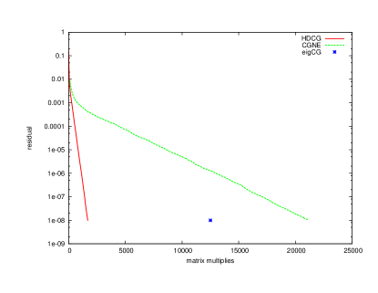
Figure 6: Residual versus fine lattice matrix multiples for the inversion of a gauge fixed wall source at physical light quark masses ($am=7.8\times 10^{-4}$) on a $48^{3}\times 96$ RBC-UKQCD configuration with lattice spacing around $a^{-1}\sim 1.73$GeV. We compare double precision conjugate gradient on the normal equations to eigCG and to HDCG. HDCG is reduces the number of fine lattice matrix multiplies by a factor of thirteen.

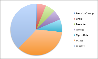
Figure 7: Components of the execution time of HDCG with the optimised parameters. Here, roughly half the time is spent in applying the fine level matrix. This time comes from both single precision applications in the $M_{IRS}$ preconditioner and double precision applications in the outer solver (labeled MprecOuter). Around one third of the time is spent solving the little Dirac operator (LdopInv) and the rest of the time is made up from linear combinations, and the promotion and projection to and from the coarsened degrees of freedom. Precision conversions constitute a small remnant contribution.

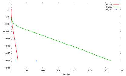
Figure 8: Wall clock execution time for the inversion of a gauge fixed wall source at physical light quark masses ($am=7.8\times 10^{-4}$) on a $48^{3}\times 96$ RBC-UKQCD configuration with lattice spacing around $a^{-1}\sim 1.73$GeV. We compare double precision conjugate gradient on the normal equations to eigCG and to HDCG. A substantial speed up is obtained with HDCG algorithm

The breakdown of the HDCG solve time is displayed as a pie chart in figure 7. As can be seen only around one half of the time is spent in fine matrix operations. Including the extra overhead, we can compare the total wall clock execution time of the different algorithms in figure 8.

Since the coarse space is a purely four dimensional treatment and does not grow with $L_{s}$, it is clear that for sufficiently large $L_{s}$ we can remove the preconditioner $M_{IRS}$ and achieve a cost effective solver that does not grow with $L_{s}$. At least with the present algorithm we are not at sufficiently large $L_{s}$ that this is a benefit, however the observation is interesting.

In table 14 we see that with only 64 vectors we see a 3.5x speed up over EigCG, and a 14.1x speedup over double precision conjugate gradient applied to the red black preconditioned normal equations. The setup time is substantially reduced compared to EigCG, and the memory footprint is an order of magnitude reduced. The case for using the algorithm is rather compelling.

Algorithm	Tolerance	Cost	Matmuls	Vectors
CGNE (double)	$10^{-8}$	1270s	21144	-
CGNE (mixed)			26000	-
EigCG (mixed)	$10^{-8}$	320s	11710	600
EigCG (mixed)	$10^{-4}$	55s	1400	600
EigCG (setup)		10h
HDCG (mixed)	$10^{-8}$	90s	1600	64
HDCG (mixed)	$10^{-4}$	30s	540	64
HDCG (setup)		2h

Table 13: We compare the performance of HDCG to existing algorithms for Mobius and domain wall Fermion solvers. A substantial speed up is obtained compared to both CGNE and to the deflated EigCG algorithm.

Comparison	Gain
Exact Solve vs CGNE	14.1x
Exact Solve vs EigCG	3.5x
Inexact Solve vs EigCG	1.8x
Setup vs EigCG	5x
Footprint vs EigCG	10x

Table 14: We compare the performance of HDCG to existing algorithms for Mobius and domain wall Fermion solvers. A substantial speed up is obtained compared to both CGNE and to the deflated EigCG algorithm.

VI.3 Convergence rate analysis

We may estimate the spectrum of the Hermitian operator using the $M_{IRS}$ polynomial to estimate the high end of the spectral range, and lowest modes of the diagonalised little Dirac operator to estimate the low end.

The lowest little Dirac operator eigenvalues treated in the second level delation lie in the interval $[2\times 10^{-5},2\times 10^{-3}]$. The highest eigenvalues of the fine operator are of $O(100)$. We would therefore estimate a condition number of order $\kappa=5\times 10^{6}$. The convergence factor bound corresponding to this condition number is

$$\sigma^{\rm predicted}(CGNE)=0.9991.$$ (38)

We measure the convergence rate from the asymptotic behaviour of CG by fitting fig 6 as

$$\sigma^{\rm measured}(CGNE)=0.9994,$$ (39)

corresponding to a condition number of $\kappa=1.2\times 10^{7}$. Given the indirect connection between the eigenvalues of our little Dirac operator and the true lowest mode of the fine Dirac operator this level of consistency is quite reasonable.

We now make make the assumption that CG bound is saturated, and use this as a reasonably accurate guide to the spectral radius of the deflated operator. After composite preconditioning with both $M_{IRS}$ polynomial preconditioner and the little Dirac operator we fit a convergence factor from fig 6 as

$$\sigma^{\rm measured}(HDCG)\sim 0.92$$ (40)

This suggests a condition number of $\kappa\sim 600$. Since the $M_{IRS}$ preconditioner is taken with $\lambda=1.0$, this the upper eigenvalue of the preconditioner matrix should lie around unity. The condition number of the preconditioner matrix suggests that eigenvalues down to around $2\times 10^{-3}$ are well treated by the little Dirac operator. This is again quite consistent with the upper end of the spectral values observed in the deflation of the little Dirac operator.

In summary: we use two complementary preconditioners designed to accurately treat the low and high ends of the spectrum respectively. The little Dirac operator appears to lift the lowest eigenvector of the preconditioned system by around two orders of magnitude from $2\times 10^{-5}$ to $2\times 10^{-3}$. The $M_{IRS}$ preconditioner reduces the highest eigenvector of the preconditioned system by a similar amount from around $100$ to around $1.0$. The combined effect is a two order of magnitude improvement in condition number and a reduction in outer iterations to around $160$. Each of these outer iterations, of course, involves around 10 matrix multiplies to implement $M_{IRS}$, with most of these matrix multiples are performed in single precision. We will demonstrate that even further reduced precision remains effective in this preconditioning in section VI.5.

VI.4 Subspace reuse

Since the subspace generation is a real investment of effort, it is interesting to consider situations where this investment can be reused. When the Dirac matrix is only modified by a small change, we have the opportunity to reuse the blocked subspace vectors. The matrix elements of the modified Dirac operator may be recomputed and the deflation space reused. Several types of modification might be considered as small perturbations for which this approach might be successful.

1. Twisted boundary conditions. The Bloch theorem suggests that to leading order in the twist the eigenvectors will simply acquire a slowly moving phase. By blocking the original vectors the large phase factors accumulated with a large translation should be absorbed.

2. Moderate changes in Fermion mass. This not obvious for five dimensional chiral Fermions as the mass is not an additive shift of the spectrum.

3. Gauge fields modified by small timesteps in a Hamiltonian update. This case has been considered by Luscher LuscherHMC and found effective. We note that this usage implies violation of reversibility at the level of convergence precision, rather than solely through rounding error accumulation at the level of the floating point precision. However, since we already use single precision arithmetic in the molecular dynamics phase of RHMC, and advocated further reduction of precision in a preconditioner (section VI.5) it is quite likely that in future reversibility violation will be controlled by convergence precision in any case.

Table 15 shows that one can indeed introduce twist angles to the gauge fields with twist up to of order one unit of Fourier momentum in each direction without significant loss of convergence. A further example can be obtained from RBC-UKQCD’s recent physical point calculation of the $K_{l3}$ form factor. The momentum required to be injected to the final state pion was included with twisted boundary conditions, and 90s was required for both the twisted and untwisted inversions with a gauge fixed wall source. This demonstrates that subspace reuse is highly effective with twisting. Table 15 also shows that one can indeed effectively reuse the subspace between different quark masses.

Algorithm	Volume	mass	Twist	Solve time
CGNE	$32^{4}$	0.01	$\frac{\pi}{L}(0,0,0)$	30s
HDCG	$32^{4}$	0.01	$\frac{\pi}{L}(0,0,0)$	6.9s
HDCG	$32^{4}$	0.01	$\frac{\pi}{L}(0.2,0,0)$	6.9s
HDCG	$32^{4}$	0.01	$\frac{\pi}{L}(0.5,0.5,0.0)$	9.2s
HDCG	$32^{4}$	0.01	$\frac{\pi}{L}(0.5,0.5,0.5)$	9.8s
HDCG	$32^{4}$	0.1	$\frac{\pi}{L}(0,0,0)$	3.6s
HDCG	$32^{4}$	0.01	$\frac{\pi}{L}(0,0,0)$	6.9s
HDCG	$32^{4}$	0.005	$\frac{\pi}{L}(0,0,0)$	7.4s
HDCG	$32^{4}$	0.001	$\frac{\pi}{L}(0,0,0)$	7.8s

Table 15: We investigate reuse of a subspace created with $m=0.01$ and with no twist in the boundary conditions for inversion of the related linear systems of equations with modest twisted boundary conditions or with modest modifications in the quark mass. These results are very encouraging.

VI.5 Reduced precision in preconditioner communication

Our $M_{IRS}$ preconditioner does have the locality benefit of SAP; the excellent communication performance in BlueGene/Q tolerates this. However motivated largely for future machines with less favourable communication performance we have investigated truncation of the floating point mantissa to only 6 bits, by truncating each single precision word to 16 bits.

Since BlueGene/Q has only IEEE floating point SIMD operations this requires moving the data through the cache between floating point and integer register files and applying a mask, rotate, or combine step; compression to 8bit is not cost effective since one is reduced to byte operations. However, the decision of how best to invest years of effort and to spend millions of dollars in future depends on definitively answering this question. This reduces the bytes per word to only two. On architectures such Xeon Phi which possess both floating point and integer SIMD operations truncation to 8 bit is feasible using a sequence of SIMD operations: maxabs, divide, and convert to 8bit signed integer instructions. In this way a 24 element four spinor could be stored as a 16bit half precision prefactor and 24 8 bit signed integers. This can potentially save a factor of eight in communication over a double precision implementation BrowerClarkeUseful .

Table 16 shows that this reduction in communication bandwidth is acheived with no algorithmic penalty in iteration count. As a consequence this appears to be an attractive competitive approach to domain decomposition; rather than suppressing communication entirely, only the most numerically significant parts of the communication are preserved.

Precision of inner communication	Exponent	Mantissa	Outer iteration count
64 bit	11 bit	52 bit	168
32 bit	8 bit	23 bit	168
16 bit	8 bit	7 bit	168

Table 16: We compare applying the $M_{IRS}$ preconditioner with different levels of numerical precision. The top two rows compare application with a uniform 64 bit and 32 bit precision of all elements of data. The final row retains 32 bit precision for all elements of data except for data communicated between nodes. The communication buffers are truncated to retain only seven mantissa bits, and no detrimental algorithmic impact is seen. Compared to the 64 bit case a four fold reduction in communication bandwidth has been achieved, however in architectures where conversion to 8bit integer can be performed in SIMD instructions we can expect successful compression by a factor near eight without loss of algorithmic efficiency.

Of course, the cache locality benefit of domain decomposition is not preserved here. However, for 5d chiral Fermions, we obtain $L_{s}$ cache reuse of gauge fields and $2N_{d}$ reuse of Fermion fields in the Dirac operator and there is already a high level of cache reuse in the matrix multiply.

The greater cache locality of domain decomposition on current machines would still improve the overall Krylov solver performance somewhat compared to HDCG since it would allow the linear combinations to be performed at cache bandwidth (rather than memory bandwidth). However the reduction of communication bandwidth achieved in this section is by far the larger effect particularly as memory technology is advancing more rapidly than interconnect technology. Consequently, it appears likely that reduced communication precision will give most of the performance benefit of domain decomposition without introducing no loss of numerical inefficiency in an inner/outer solver.

VII Conclusions

In this paper we have developed an inexact deflation method to accelerating the red-black preconditioned normal equations. The matrices studied have a forty times larger stencil required compared to the nearest neighbour non-Hermitian stencil that is used with Wilson and clover Fermions. We introduced required several substantial algorithmic refinements, in order to give a real speed up in algorithm running time.

The use of the ADEF-2 algorithm allowed improved robustness to loose convergence of the little Dirac operator, but with no formal change in convergence compared to the Schur complement algorithm first implemented in inexact deflationLuscher:2007se . This reduced the little Dirac operator overhead by a factor of ten. The preconditioned conjugate gradient solver is remarkably tolerant to preconditioner variability, and this organisation of the matrices almost eliminates the need for flexible algorithms.

The generation and use of additional deflation space vectors in a hierarchical multi-level deflation further reduced the cost of the coarse space by a factor between three and ten. The grid pattern here continues to mirror Luscher’s original algorithm with a $1^{4}$ third grid.

We introduced an infra-red shift preconditioner based on a fixed number of CG iterations to replace the Schwarz procedure used in both Luscher’s approach and in the multigrid papers. This preconditioner has been demonstrated

A further factor of three reduction in little Dirac operator overhead was obtained by using an infra-red shift preconditioner based on the truncation of our little Dirac operator to nearest neighbour. This reduced the bulk of coarse grid matrix multiplies to the same stencil as in the Wilson case.

Since the coarse space is represented as a purely four dimensional system, we have perhaps taken an important step towards alleviating $L_{s}$ scaling of 5d Chiral Fermions.

VIII Acknowledgements

All simulations in this work were performed on the STFC DiRAC BlueGene/Q facility in Edinburgh. This work was supported by grants ST/K005790/1, ST/K005804/1, ST/K000411/1, ST/H008845/1, STFC Grant ST/J000329/1 and the European Union ITN StrongNET (Agreement 238353). The author particularly wishes to thank Martin Luscher, Mike Clark, Richard Brower, Andreas Juettner, Marina Marinkovic and my colleagues in RBC and in UKQCD for useful conversations in both audible and electronic forms.

References

- (1) M. F. Atiyah and I. M. Singer. “The index of elliptic operators on compact manifolds”. Bull. Amer. Math. Soc. 69 (1963), 422-433
- (2) L. S. Brown, R. D. Carlitz and C. -k. Lee, “Massless Excitations in Instanton Fields,” Phys. Rev. D 16 (1977) 417.
- (3) M. Hestenes and E. Stiefel. “Methods of Conjugate Gradients for Solving Linear Systems”. Journal of Research of the National Bureau of Standards. V49 No 6 P409 Dec (1952).
- (4) Section 6.11, Y. Saad. 2003. Iterative Methods for Sparse Linear Systems (2nd ed.). Soc. for Industrial and Applied Math., Philadelphia, PA, USA,
- (5) R. B. Morgan and W. Wilcox, Nucl. Phys. Proc. Suppl. 106 (2002) 1067 [hep-lat/0109009].
- (6) D. Darnell, R. B. Morgan and W. Wilcox, Nucl. Phys. Proc. Suppl. 129 (2004) 856 [hep-lat/0309068].
- (7) D. Darnell, R. B. Morgan and W. Wilcox, Linear Algebra Appl. 429 (2008) 2415 [arXiv:0707.0502 [math-ph]].
- (8) A. Stathopoulos and K. Orginos, SIAM J. Sci. Comput. 32 (2010) 439 [arXiv:0707.0131 [hep-lat]].
- (9) A. Brandt. Math. Comp., 31:333–390, 1977.
- (10) M. Luscher, “Local coherence and deflation of the low quark modes in lattice QCD,” JHEP 0707 (2007) 081 [arXiv:0706.2298 [hep-lat]].
- (11) M. Brezina, R. Falgout, S. MacLachlan, T. Manteuffel, S. McCormick, and J. Ruge, “Adaptive Smoothed Aggregation (SA)”, SIAM J. Sci. Comput., 25(6), 1896–1920.
- (12) J. Brannick, R. C. Brower, M. A. Clark, J. C. Osborn and C. Rebbi, “Adaptive Multigrid Algorithm for Lattice QCD,” Phys. Rev. Lett. 100 (2008) 041601 [arXiv:0707.4018 [hep-lat]].
- (13) J. Brannick, R. C. Brower, M. A. Clark, J. C. Osborn and C. Rebbi, “Adaptive Multigrid Algorithm for the QCD Dirac-Wilson Operator,” PoS LAT 2007 (2007) 029 [arXiv:0710.3612 [hep-lat]].
- (14) M. A. Clark, J. Brannick, R. C. Brower, S. F. McCormick, T. A. Manteuffel, J. C. Osborn and C. Rebbi, “The Removal of critical slowing down,” PoS LATTICE 2008 (2008) 035 [arXiv:0811.4331 [hep-lat]].
- (15) R. Babich, J. Brannick, R. C. Brower, M. A. Clark, S. D. Cohen, J. C. Osborn and C. Rebbi, “The Role of multigrid algorithms for LQCD,” PoS LAT 2009 (2009) 031 [arXiv:0912.2186 [hep-lat]].
- (16) R. Babich, J. Brannick, R. C. Brower, M. A. Clark, T. A. Manteuffel, S. F. McCormick, J. C. Osborn and C. Rebbi, “Adaptive multigrid algorithm for the lattice Wilson-Dirac operator,” Phys. Rev. Lett. 105 (2010) 201602 [arXiv:1005.3043 [hep-lat]].
- (17) J. C. Osborn, R. Babich, J. Brannick, R. C. Brower, M. A. Clark, S. D. Cohen and C. Rebbi, “Multigrid solver for clover fermions,” PoS LATTICE 2010 (2010) 037 [arXiv:1011.2775 [hep-lat]].
- (18) A. Frommer, K. Kahl, S. Krieg, B. Leder and M. Rottmann, “Aggregation-based Multilevel Methods for Lattice QCD,” PoS LATTICE 2011 (2011) 046 [arXiv:1202.2462 [hep-lat]].
- (19) A. Frommer, K. Kahl, S. Krieg, B. ör. Leder and M. Rottmann, “Adaptive Aggregation Based Domain Decomposition Multigrid for the Lattice Wilson Dirac Operator,” arXiv:1303.1377 [hep-lat].
- (20) A. Frommer, K. Kahl, S. Krieg, B. Leder and M. Rottmann, “An adaptive aggregation based domain decomposition multilevel method for the lattice wilson dirac operator: multilevel results,” arXiv:1307.6101 [hep-lat].
- (21) S. D. Cohen, R. C. Brower, M. A. Clark and J. C. Osborn, “Multigrid Algorithms for Domain-Wall Fermions,” PoS LATTICE 2011 (2011) 030 [arXiv:1205.2933 [hep-lat]].
- (22) D. B. Kaplan, “A Method for simulating chiral fermions on the lattice,” Phys. Lett. B 288 (1992) 342 [hep-lat/9206013].
- (23) Y. Shamir, “Chiral fermions from lattice boundaries,” Nucl. Phys. B 406 (1993) 90 [hep-lat/9303005].
- (24) V. Furman and Y. Shamir, “Axial symmetries in lattice QCD with Kaplan fermions,” Nucl. Phys. B 439 (1995) 54 [hep-lat/9405004].
- (25) R. Narayanan and H. Neuberger, “Chiral determinant as an overlap of two vacua,” Nucl. Phys. B 412 (1994) 574 [hep-lat/9307006].
- (26) R. Narayanan and H. Neuberger, “Chiral fermions on the lattice,” Phys. Rev. Lett. 71 (1993) 3251 [hep-lat/9308011].
- (27) R. Narayanan and H. Neuberger, “A Construction of lattice chiral gauge theories,” Nucl. Phys. B 443 (1995) 305 [hep-th/9411108].
- (28) H. Neuberger, “Exactly massless quarks on the lattice,” Phys. Lett. B 417 (1998) 141 [hep-lat/9707022].
- (29) H. Neuberger, “Vector - like gauge theories with almost massless fermions on the lattice,” Phys. Rev. D 57 (1998) 5417 [arXiv:hep-lat/9710089].
- (30) Y. Kikukawa and T. Noguchi, “Low-energy effective action of domain wall fermion and the Ginsparg-Wilson relation,” hep-lat/9902022.
- (31) A. Borici, “Truncated overlap fermions,” Nucl. Phys. Proc. Suppl. 83 (2000) 771 [hep-lat/9909057].
- (32) A. Borici, “Truncated overlap fermions: The Link between overlap and domain wall fermions,” hep-lat/9912040.
- (33) R. C. Brower, H. Neff and K. Orginos, “Mobius fermions: Improved domain wall chiral fermions,” Nucl. Phys. Proc. Suppl. 140 (2005) 686 [hep-lat/0409118].
- (34) R. G. Edwards, B. Joo, A. D. Kennedy, K. Orginos and U. Wenger, “Comparison of chiral fermion methods,” PoS LAT 2005 (2006) 146 [hep-lat/0510086].
- (35) R. C. Brower, H. Neff and K. Orginos, arXiv:1206.5214 [hep-lat].
- (36) N. M. Nachtigal, S. C. Reddy, and L. N. Trefethen, “How Fast are Nonsymmetric Matrix Iterations?” SIAM. J. Matrix Anal. & Appl., 13(3), 778–795.
- (37) Rudy Arthur, PhD Thesis.
-
(38)
O. Axelsson, “On preconditioning and convergence acceleration in sparse matrix problems”,
CERN, 1974. - 21 p. DOI:10.5170/CERN-1974-010
P. Concus, G.H. Golub, and D.P. O’Leary, “A generalized conjugate gradient method for the numerical solution of elliptic partial differential equations”, in Sparse Matrix Computations, J.R. Bunch and D.J. Rose, eds., Acadmeic Press, NY, 1976, pp. 309-332 - (39) Page 278, Y. Saad. 2003. “Iterative Methods for Sparse Linear Systems” (2nd ed.). Soc. for Industrial and Applied Math., Philadelphia, PA, USA,
- (40) Diane P. O’Leary, “Yet another polynomial preconditioner for the conjugate gradient algorithm”, Linear Algebra and its Applications Volumes 154–156, August–October 1991, Pages 377–388
- (41) G. H. Golub and Q. Ye, “Inexact preconditioned conjugate gradient method with inner-outer iteration” Siam J. Sci. Comput. Vol. 21, No. 4, pp. 1305–1320
- (42) Yvan Notay, “Flexible conjugate gradients”, SIAM J. Sci. Comput, (2000), Vol. 22, p1444.
- (43) J. M. Tang, R. Nabben, C. Vuik, Y. A. Erlangga, “Comparison of Two-Level Preconditioners Derived from Deflation, Domain Decomposition and Multigrid Methods” Journal of Scientific Computing June 2009, Volume 39, Issue 3, pp 340-370
- (44) “The ibm blue gene/q compute chip” Haring, Ruud A and Ohmacht, Martin and Fox, Thomas W and Gschwind, Michael K and Satterfield, David L and Sugavanam, Krishnan and Coteus, Paul W and Heidelberger, Philip and Blumrich, Matthias A and Wisniewski, Robert W and others, IEEE Micro, V32.2 p48 (2012)
- (45) P. A. Boyle, “The BlueGene/Q supercomputer,” PoS LATTICE 2012 (2012) 020.
- (46) P. A. Boyle, “The BAGEL assembler generator”, Computer Physics Communications 180/12:2739 (2009) [doi:10.1016/j.cpc.2009.08.010]
- (47) T. Blum, T. Izubuchi and E. Shintani, “Error reduction technique using covariant approximation and application to nucleon form factor,” PoS LATTICE 2012 (2012) 262 [arXiv:1212.5542].
- (48) E. Shintani, R. Arthur, T. Blum, T. Izubuchi, C. Jung and C. Lehner, “Covariant approximation averaging,” arXiv:1402.0244 [hep-lat].
- (49) Mike Clark and Richard Brower, useful conversations regarding reduced precision storage schemes for intermediate fields.
- (50) M. Luscher, “Deflation acceleration of lattice QCD simulations,” JHEP 0712 (2007) 011 [arXiv:0710.5417 [hep-lat]].