Coordinated Output Regulation of Heterogeneous Linear Systems under Switching Topologies

Abstract

This paper constructs a framework to describe and study the coordinated output regulation problem for multiple heterogeneous linear systems. Each agent is modeled as a general linear multiple-input multiple-output system with an autonomous exosystem which represents the individual offset from the group reference for the agent. The multi-agent system as a whole has a group exogenous state which represents the tracking reference for the whole group. Under the constraints that the group exogenous output is only locally available to each agent and that the agents have only access to their neighbors’ information, we propose observer-based feedback controllers to solve the coordinated output regulation problem using output feedback information. A high-gain approach is used and the information interactions are allowed to be switched over a finite set of fixed networks containing both graphs that have a directed spanning tree and graphs that do not. The fundamental relationship between the information interactions, the dwell time, the non-identical dynamics of different agents, and the high-gain parameters is given. Simulations are shown to validate the theoretical results.

, , ,

1 Introduction

Coordinated control of multi-agent systems has recently drawn large attention due to its broad applications in physical, biological, social, and mechanical systems [2, 3, 4, 5]. The key idea of “coordination” algorithm is to realize a global emergence using only local information interactions [6, 7]. The coordination problem of a single-integrator network is fully studied with an emphasis on the system robustness to the input time delays and switching communication topologies [6, 7, 8, 9], discrete-time dynamical models [10, 11], nonlinear couplings [12], the convergence speed evaluation [13], the effects of quantization [14], and the leader-follower tracking [15].

Following these ideas, the study of coordination of multiple linear dynamic systems becomes an attractive and fruitful research direction for the control community recently. For example, the authors of [16] generalize the existing works on coordination of multiple single-integrator systems to the case of multiple linear time-invariant single-input systems. For a network of neutrally stable systems and polynomially unstable systems, the author of [17] proposes a design scheme for achieving synchronization. The case of switching communication topologies is considered in [18] and a so-called consensus-based observer is proposed to guarantee leaderless synchronization of multiple identical linear dynamic systems under a jointly connected communication topology. Similar problems are also considered in [19] and [20], where a frequently connected communication topology is studied in [19] and an assumption on the neutral stability is imposed in [20]. The authors of [21] propose a neighbor-based observer to solve the synchronization problem for general linear time-invariant systems. An individual-based observer and a low-gain technique are used in [22] to synchronize a group of linear systems with open-loop poles at most polynomially unstable. In addition, the classical Laplacian matrix is generalized in [23] to a so-called interaction matrix. A D-scaling approach is then used to stabilize this interaction matrix under both fixed and switching communication topologies. Synchronization of multiple heterogeneous linear systems has been investigated under both fixed and switching communication topologies [24, 25, 26]. A similar problem is studied in [27, 28], where a high-gain approach is proposed to dominate the non-identical dynamics of the agents. The cases of frequently connected and jointly connected communication topologies are studied in [29] and [30], respectively, where a slow switching condition and a fast switching condition are presented. Recently, the generalizations of coordination of multiple linear dynamic systems to the cooperative output regulation problem are studied in [31, 32, 33]. In addition, the study on the synchronization of homogenous or heterogeneous networks with nonlinear couplings also attracts extensive attention [34, 35, 36, 37].

In this paper, we generalize the classical output regulation problem of an individual linear dynamic system to the coordinated output regulation problem of multiple heterogeneous linear dynamic systems. We consider the case where each agent has an individual offset and simultaneously there is a group tracking reference. The individual offset and the group reference are generated by autonomous systems (i.e., systems without inputs). Each individual offset is available to its corresponding agent while the group reference can be obtained only through constrained communication among the agents, i.e., the group reference trajectory is available to only a subset of the agents. Our goal is to find an observer-based feedback controller for each agent such that the output of each agent converges to a given trajectory determined by the combination of the individual offset and the group reference. Motivated by the approach proposed in [27], we propose a unified observer to solve the coordinated output regulation problem of multiple heterogeneous general linear dynamics, where the open-loop poles of the agents can be exponentially unstable and the dynamics are allowed to be different both with respect to dimensions and parameters. This relaxes the common assumption of identical dynamics [17, 18, 20, 21, 29] or open-loop poles at most polynomially unstable [18, 20, 26]. The main contribution of this work is that the information interaction is allowed to be switching from a graph set containing both a directed spanning tree set and a disconnected graph set for the case of heterogeneous linear systems. This extends the existing works on the case of fixed communication topologies [17, 21, 27, 31]. The high-gain technique is used and the relationships between the dwell time [38], the non-identical dynamics among different agents and the high-gain parameters are also given.

The remainder of the paper is organized as follows. In Section 2, we give some basic definitions on network model. In Section 3, we formulate the problem of coordinated output regulation of multiple heterogenous linear systems. We then propose the state feedback control law with a unified observer design in Section 4. Two case studies are given in Section 5. Numerical studies are carried out in Section 6 to validate our designs of observer-based controllers and a brief concluding remark is drawn in Section 7.

2 Network Model

We use graph theory to model the communication topology among agents. A directed graph ${G}$ consists of a pair $(\mathbf{{V}},\mathbf{{E}})$, where $\mathbf{{V}}=\{\nu_{1},\nu_{2},\ldots,\nu_{n}\}$ is a finite, nonempty set of nodes and $\mathbf{{E}}\subseteq\mathbf{{V}}\times\mathbf{{V}}$ is a set of ordered pairs of nodes. An edge $(\nu_{i},\nu_{j})$ denotes that node $\nu_{j}$ can obtain information from node $\nu_{i}$. All neighbors of node $\nu_{i}$ are denoted as $N_{i}:=\{\nu_{j}|(\nu_{j},\nu_{i})\in\mathbf{{E}}\}$. For an edge $(\nu_{i},\nu_{j})$ in a directed graph, $\nu_{i}$ is the parent node and $\nu_{j}$ is the child node. A directed path in a directed graph is a sequence of edges of the form $(\nu_{i},\nu_{j}),(\nu_{j},\nu_{k}),\ldots$. A directed tree is a directed graph, where every node has exactly one parent except for one node, called the root, which has no parent, and the root has a directed path to every other node. A directed graph has a directed spanning tree if there exists at least one node having a directed path to all other nodes.

For a leader-follower graph $\overline{{G}}:=(\overline{{V}},\overline{{E}})$, we have $\overline{{V}}=\{\nu_{0},\nu_{1},\dots,\nu_{n}\}$, $\overline{{E}}\subseteq\overline{{V}}\times\overline{{V}}$, where $\nu_{0}$ is the leader and $\nu_{1},\nu_{2},\ldots,\nu_{n}$ denote the followers. The leader-follower adjacency matrix $\overline{{A}}=[a_{ij}]\in\mathbb{R}^{(n+1)\times(n+1)}$ is defined such that $a_{ij}$ is positive if $(\nu_{j},\nu_{i})\in\overline{{E}}$ while $a_{ij}=0$ otherwise. Here we assume that $a_{ii}=0$, $i=0,1,\dots,n$, and the leader has no parent, i.e., $a_{0j}=0,j=0,1,\cdots,n$. The leader-follower “grounded” Laplacian matrix $L=[l_{ij}]\in\mathbb{R}^{{n\times n}}$ associated with $\overline{{A}}$ is defined as $l_{ii}=\sum_{j=0}^{n}a_{ij}$ and $l_{ij}=-a_{ij}$, where $i\neq j$.

In this paper, we assume that the leader-follower communication topology $\overline{{G}}_{\sigma(t)}$ is time-varying and switching from a finite set $\{\overline{{G}}_{k}\}_{k\in\Gamma}$, where $\Gamma=\{1,2,\dots,\delta\}$ is an index set and $\delta\in\mathbb{N}$ indicates its cardinality. We impose the technical condition that $\overline{{G}}_{\sigma(t)}$ is right continuous, where ${\sigma}:[t_{0},\infty)\rightarrow\Gamma$ is a piecewise constant function of time. That is to say, $\overline{{G}}_{\sigma(t)}$ remains constant for $t\in[t_{\ell},t_{\ell+1})$, $\ell=0,1,\dots$ and switches at $t=t_{\ell}$, $\ell=1,2,\dots$. In addition, we assume that $\inf_{\ell}(t_{\ell+1}-t_{\ell})\geq\tau_{d}>0$, $\ell=0,1,\dots$, with $\lim_{\ell\rightarrow\infty}t_{\ell}=\infty$, where $\tau_{d}$ is a constant known as the dwell time [38].

Let the sets $\{\overline{{A}}_{k}\}_{k\in\Gamma}$ and $\{L_{k}\}_{k\in\Gamma}$ be the leader-follower adjacency matrices and leader-follower grounded Laplacian matrices associated with $\{\overline{{G}}_{k}\}_{k\in\Gamma}$, respectively. Consequently, the time-varying leader-follower adjacency matrix and time-varying leader-follower grounded Laplacian matrix are defined as $\overline{{A}}_{\sigma(t)}=[a_{ij}(t)]$ and $L_{\sigma(t)}=[l_{ij}(t)]$.

Other notation in this paper: $\lambda_{\min}(P)$ and $\lambda_{\max}(P)$ denote, respectively, the minimum and maximum eigenvalues of a real symmetric matrix $P$, $P^{\rm\tiny T}$ denotes the transpose of $P$, and $I_{n}$ denotes the $n\times n$ identity matrix.

3 Problem Formulation

3.1 Agent Dynamics

Suppose that we have $n$ agents modeled by the linear MIMO systems:

$$\dot{x}_{i}=A_{i}x_{i}+B_{i}u_{i},$$ (1)

where $x_{i}\in\mathbb{R}^{n_{i}}$ is the agent state, $u_{i}\in\mathbb{R}^{m_{i}}$ is the control input, $A_{i}\in\mathbb{R}^{n_{i}\times n_{i}}$, and $B_{i}\in\mathbb{R}^{n_{i}\times m_{i}}$.

Also suppose that there is an individual autonomous exosystem for each $\nu_{i}\in\mathbf{V}$,

$$\dot{\omega}_{i}=S_{i}\omega_{i},$$ (2)

where $\omega_{i}\in\mathbb{R}^{q_{i}}$ and $S_{i}\in\mathbb{R}^{q_{i}\times q_{i}}$.

In addition, there is a group autonomous exosystem for the multi-agent system as a whole:

$$\dot{x}_{0}=A_{0}x_{0},$$ (3)

where $x_{0}\in\mathbb{R}^{n_{0}}$ and $A_{0}\in\mathbb{R}^{n_{0}\times n_{0}}$.

3.2 Control Architecture

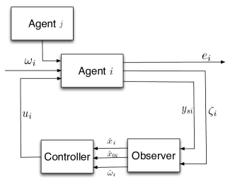
Figure 1: Control architecture for agent $\nu_{i}$

The control of each agent is supposed to have the structure shown in Fig. 1. More specifically, for the individual autonomous exosystem tracking, available output information for agent $\nu_{i}\in\mathbf{V}$ is

$$y_{si}=C_{si}x_{i}+C_{wi}\omega_{i},$$

where $C_{si}\in\mathbb{R}^{p_{1}\times n_{i}}$, and $C_{wi}\in\mathbb{R}^{p_{1}\times q_{i}}$.

For the group autonomous exosystem tracking, only neighbor-based output information is available due to the constrained communication. This means that not all the agents have access to $y_{0}$. The available information is the neighbor-based sum of each agent’s own output relative to that of its’ neighbors, i.e.,

$$\zeta_{i}=\sum_{j=0}^{n}a_{ij}(t)(y_{di}-y_{dj})$$

is available for each agent $\nu_{i}\in\mathbf{V}$, where $a_{ij}(t)$, $i=0,1,\ldots,n$, $j=0,1,\ldots,n$, is entry $(i,j)$ of the adjacency matrix $\overline{{A}}_{\sigma(t)}$ associated with $\overline{{G}}_{\sigma(t)}$ defined in Section 2 at time $t$, $y_{di}$ can be represented by $y_{di}=C_{di}x_{i}$, $i=1,2,\dots,n$ and $y_{d0}=C_{0}x_{0}$, where $C_{di}\in\mathbb{R}^{p_{2}\times n_{i}}$, $i=1,2,\dots,n$ and $C_{0}\in\mathbb{R}^{p_{2}\times n_{0}}$. Also, the relative estimation information is available using the same communication topologies, i.e.,

$$\widehat{\zeta}_{i}=\sum_{j=0}^{n}a_{ij}(t)(\widehat{y}_{i}-\widehat{y}_{j})$$

is available for each agent $\nu_{i}\in\mathbf{V}$, where $\widehat{y}_{i}$ is an estimation produced internally by each agent $\nu_{i}\in\mathbf{V}$.

Fig. 2 gives an example of information flow among the agents and the group autonomous exosystem $\nu_{0}$ for $n=3$ agents.

3.3 Switching Topologies

For the communication topology set $\{\overline{{G}}_{k}\}_{k\in\Gamma}$, we assume that $\overline{{G}}_{k}$, $\forall k\in\Gamma_{c}$ is a graph containing a directed spanning tree with $\nu_{0}$ rooted. Without loss of generality, we relabel $\Gamma_{c}:=\{1,2,\dots,\delta_{1}\}$ ($1\leq\delta_{1}\leq\delta$), where $\delta_{1}\in\mathbb{N}$. The remaining graphs are labeled as $\overline{{G}}_{k}$, $\forall k\in\Gamma_{d}$, where $\Gamma_{d}:=\{\delta_{1}+1,\delta_{1}+2,\dots,\delta\}$. Denote the graph set $\overline{\mathbb{G}}_{c}=\{\overline{{G}}_{k}\}_{k\in\Gamma_{c}}$ and the graph set $\overline{\mathbb{G}}_{d}=\{\overline{{G}}_{k}\}_{k\in\Gamma_{d}}$, respectively. We also denote $T^{d}_{\overline{t}_{0}}(t)$ and $T_{\overline{t}_{0}}^{c}(t)$ the total activation time when $\overline{{G}}_{\sigma(\varsigma)}\in\overline{\mathbb{G}}_{d}$ and total activation time when $\overline{{G}}_{\sigma(\varsigma)}\in\overline{\mathbb{G}}_{c}$ during $\varsigma\in[\overline{t}_{0},t)$ for $\overline{t}_{0}\geq t_{0}$.

Assumption 1.

The dwell time $\tau_{d}$ is a positive constant.

Assumption 2.

Given a positive constant $\kappa$, there exists a $\overline{t}_{0}\geq t_{0}$ such that $T^{c}_{\overline{t}_{0}}(t)\geq\kappa T^{d}_{\overline{t}_{0}}(t)$ for all $t\geq\overline{t}_{0}$.

Remark 1.

Note that a sufficient condition satisfying Assumption 2 is that $\overline{\mathbb{G}}_{c}$ is non-empty and given a $T>0$ and $\tau_{d}>0$, for any $t\geq t_{0}$, the switching signal $\sigma(t)$ satisfies $\{t|\overline{{G}}_{\sigma(t)}\in\overline{\mathbb{G}}_{c}\}\cap[t,t+T]\neq\emptyset$. Such a condition is also referred as “frequently connected” condition (i.e., the communication topology that contains a directed spanning tree is active frequently enough [19, 23]). Note that this condition implies that there exists a time sequence $0=T_{0}<T_{1}<\dots<T_{\ell}\dots$ such that $\{t|\overline{{G}}_{\sigma(t)}\in\overline{\mathbb{G}}_{c}\}\cap[T_{\ell},T_{\ell+1}]\neq\emptyset$, for all $\ell=0,1,\dots$, where $T_{\ell+1}-T_{\ell}\leq 2T$. Therefore, there exists a $\overline{t}_{0}\in[t_{0},t_{0}+2T]$ such that $T^{c}_{\overline{t}_{0}}(t)\geq\frac{\tau_{d}}{2T}T^{d}_{\overline{t}_{0}}(t)$ for all $t\geq\overline{t}_{0}$.

3.4 Control Objective

The control objective of each agent is to track a given trajectory determined by the combination of the group reference $x_{0}$ and the individual offset $\omega_{i}$, $i=1,2,\dots,n$. Such a combination is captured by the coordinated output regulation tracking error (i.e., the total tracking error representing the combination of both individual tracking and group tracking of each agent):

$$e_{i}=D_{si}x_{i}+D_{wi}\omega_{i}+D_{0}x_{0}.$$ (4)

Thus, our objective is to guarantee that $\lim_{t\rightarrow\infty}e_{i}(t)=0$. We design an observer-based controller with available individual output information and neighbor-based group output information to solve this problem.

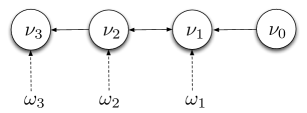
Figure 2: Information flow associated with three agents $\nu_{1}$, $\nu_{2}$, $\nu_{3}$, the individual autonomous exosystems $\omega_{1}$, $\omega_{2}$, $\omega_{3}$, and the group autonomous exosystem $\nu_{0}$

For the system shown in Fig. 2, the overall control can correspond to a formation control problem, where $\omega_{i}$ encodes the relative position between each agent and the leader while the leader $x_{0}$ defines the overall motion of the group.

4 Coordinated Output Regulation with Unified Observer Design

As suggested by Fig. 1, the design procedure to solve the coordinated output regulation problem includes two main steps: the first one is the state feedback control design and the second one is the observer design for the group autonomous exosystem, the individual autonomous exosystem, and internal state information for each agent.

4.1 Redundant Modes

Before designing state feedback control and distributed observer, we need first to remove the redundant modes that have no effect on $y_{si}$ and $y_{di}-y_{d0}$.

We impose the following assumptions on the structure of the systems.

Assumption 3.

$\bullet$ $\left(A_{i},\left[\begin{array}[]{c}C_{si}\\ C_{di}\end{array}\right]\right)$, $i=1,2,\dots,n$ is observable.
$\bullet$ $(S_{i},C_{wi})$, $i=1,2,\dots,n$ is observable.
$\bullet$ $(A_{0},C_{0})$, $i=1,2,\dots,n$ is observable.

We first write the state and output of each agent in the compact form

$$\left[\begin{array}[]{c}\dot{x}_{i}\\ \dot{\omega}_{i}\\ \dot{x}_{0}\end{array}\right] =\left[\begin{array}[]{ccc}A_{i}&0&0\\ 0&S_{i}&0\\ 0&0&A_{0}\end{array}\right]\left[\begin{array}[]{c}x_{i}\\ \omega_{i}\\ x_{0}\end{array}\right]+\left[\begin{array}[]{c}B_{i}\\ 0\\ 0\end{array}\right]u_{i},$$

$$\left[\begin{array}[]{c}y_{si}\\ y_{di}-y_{d0}\end{array}\right] =\left[\begin{array}[]{ccc}C_{si}&C_{wi}&0\\ C_{di}&0&-C_{0}\end{array}\right]\left[\begin{array}[]{c}x_{i}\\ \omega_{i}\\ x_{0}\end{array}\right].$$

Given that Assumption 3 is satisfied, we can perform the state transformation given in Step 1 of [27] by considering $\omega_{i}$ and $x_{0}$ together. We can construct a new state $\overline{x}_{i}=W_{i}\left[\begin{array}[]{c}x_{i}\\ \omega_{i}\\ x_{0}\end{array}\right]$ with the dynamics

$$\dot{\overline{x}}_{i} =\overline{A}_{i}\overline{x}_{i}+\overline{B}_{i}u_{i}=\left[\begin{array}[]{cc}A_{i}&\overline{A}_{i12}\\ 0&\overline{A}_{i22}\end{array}\right]\overline{x}_{i}+\left[\begin{array}[]{c}B_{i}\\ 0\end{array}\right]u_{i},$$ (6e)

$$\left[\begin{array}[]{c}y_{si}\\ e_{di}\end{array}\right] =\overline{C}_{i}\overline{x}_{i}=\left[\begin{array}[]{cc}C_{si}&\overline{C}_{i21}\\ C_{di}&\overline{C}_{i22}\end{array}\right]\overline{x}_{i}.$$ (6j)

where $e_{di}=y_{di}-y_{d0}$, and the details designs on $W_{i}$, $\overline{A}_{i}$, $\overline{B}_{i}$, $\overline{C}_{i}$ are given in [27]. It was shown that pair $(\overline{A}_{i},\overline{C}_{i})$ is observable and the eigenvalues of $\overline{A}_{i22}$ are a subset of the eigenvalues of $S_{i}$ and $A_{0}$, $i=1,2,\dots,n$.

4.2 Regulated State feedback Control Law

We now design a controller to regulate $e_{i}$ to zero for each agent based on the state information $\overline{x}_{i}=\left[\begin{array}[]{c}\overline{x}_{i1}\\ \overline{x}_{i2}\end{array}\right]$, where $\overline{x}_{i1}\in\mathbb{R}^{n_{i}}$.

We impose the following assumptions on the structure of the systems.

Assumption 4.

$\bullet$ $(A_{i},B_{i})$ is stabilizable, $i=1,\dots,n$. $\bullet$ $(A_{i},B_{i},D_{si})$ is right-invertible, $i=1,\dots,n$. $\bullet$ $(A_{i},B_{i},D_{si})$ has no invariant zeros in the closed right-half complex plane that coincide with the eigenvalues of $S_{i}$ or $A_{0}$, $i=1,\dots,n$.

Lemma 1.

Let Assumption 4 hold. Then, the regulator equations (7) are solvable and the state-feedback controller $u_{i}=F_{i}(\overline{x}_{i1}-\Pi_{i}\overline{x}_{i2})+\Gamma_{i}\overline{x}_{i2}$ ensures that $\lim_{t\rightarrow\infty}e_{i}(t)=0$, $i=1,2\ldots,n$, where $\Pi_{i}$, $\Gamma_{i}$ are the solutions of the following regulator equations

$$\Pi_{i}\overline{A}_{i22} =A_{i}\Pi_{i}+\overline{A}_{i12}+B_{i}\Gamma_{i},$$ (7a)

$$0 =D_{si}\Pi_{i}+\left[\begin{array}[]{cc}D_{wi}&D_{0}\end{array}\right],\quad i=1,2\dots,n,$$ (7c)

and $F_{i}$ is chosen such that $A_{i}+B_{i}F_{i}$ is Hurwitz.

Proof.

It follows from [39] and the similar analysis of proof of Lemma 3 in [27], we can show that the regulator equations (7) are solvable given that Assumption 4 is satisfied. Then, by considering $\dot{\overline{x}}_{i2}=\overline{A}_{i22}\overline{x}_{i2}$ as the exosystem and $\dot{x}_{i}=A_{i}x_{i}+B_{i}u_{i}$ as the system to be regulated for the classic output regulation result [40], we know that $u_{i}=F_{i}(\overline{x}_{i1}-\Pi_{i}\overline{x}_{i2})+\Gamma_{i}\overline{x}_{i2}$ ensures that $\lim_{t\rightarrow\infty}e_{i}(t)=0$, $i=1,2\ldots,n$, where $\Pi_{i}$ and $\Gamma_{i}$ are the solutions of the regulator equations (7). ∎

We next design observers to estimate $\overline{x}_{i}$ based on output information $y_{si}$ and $\zeta_{i}$ for each agent.

4.3 Pseudo-identical Linear Transformation

Note that the individual offset $\omega_{i}$ can be estimated by $y_{si}$ and the group reference $x_{0}$ can be estimated by $\widehat{\zeta}_{i}$. In contrast, the internal state information $x_{i}$ for each agent can be obtained by either $y_{si}$ or $\widehat{\zeta}_{i}$. In this section, we use the combination of $y_{si}$ and $\widehat{\zeta}_{i}$ to give a unified observer design.

We define $\chi_{i}=T_{i}\overline{x}_{i}\in\mathbb{R}^{p\overline{n}}$, $i=1,2,\dots,n$, where $\overline{n}=n_{0}+\max_{i=1,2,\dots,n}(n_{i}+q_{i})$, $p=p_{1}+p_{2}$, and

$$T_{i}=\left[\begin{array}[]{c}\overline{C}_{i}\\ \vdots\\ \overline{C}_{i}\overline{A}_{i}^{\overline{n}-1}\end{array}\right].$$

Note that $T_{i}$ is full column rank since the pair $(\overline{A}_{i},\overline{C}_{i})$, $i=1,2,\dots,n$ is observable. This implies that $T_{i}^{\rm\tiny T}T_{i}$ is nonsingular. Therefore, it follows that

$$\dot{\chi}_{i} =(\mathcal{A}+\mathcal{L}_{i})\chi_{i}+\mathcal{B}_{i}u_{i},$$ (8a)

$$\left[\begin{array}[]{c}y_{si}\\ e_{di}\end{array}\right] =\mathcal{C}\chi_{i},\quad i=1,2,\dots,n,$$ (8d)

where $\mathcal{A}=\left[\begin{array}[]{cc}0&I_{p(\overline{n}-1)}\\ 0&0\end{array}\right]\in\mathbb{R}^{p\overline{n}\times p\overline{n}}$, $\mathcal{L}_{i}=\left[\begin{array}[]{c}0\\ L_{i}\end{array}\right]$, $\mathcal{B}_{i}=T_{i}\overline{B}_{i}$, $\mathcal{C}=\left[\begin{array}[]{cc}I_{p}&0\end{array}\right]\in\mathbb{R}^{p\times p\overline{n}}$ for some matrix $L_{i}\in\mathbb{R}^{p\times p\overline{n}}$.

4.4 Unified Observer Design

Motivated by [27], based on the available output information $y_{si}$ and the neighbor-based group output information $\zeta_{i}$, the distributed observer is proposed for (8) as

$$\dot{\widehat{\chi}}_{i}=(\mathcal{A}+\mathcal{L}_{i})\widehat{\chi}_{i}+\mathcal{B}_{i}u_{i}+S(\varepsilon)\mathcal{P}\mathcal{C}^{\rm\tiny T}$$

$$\times\left(\left[\begin{array}[]{c}y_{si}\\ \sum_{j=0}^{n}a_{ij}(t)(y_{di}-y_{dj})\end{array}\right]-\left[\begin{array}[]{c}\widehat{y}_{si}\\ \sum_{j=0}^{n}a_{ij}(t)(\widehat{y}_{i}-\widehat{y}_{j})\end{array}\right]\!\!\right),$$ (13)

$$\qquad\qquad\qquad\qquad\qquad\qquad i=1,2\ldots,n,$$ (14)

where $a_{ij}(t)$, $i=0,1,\ldots,n$, $j=0,1,\ldots,n$, is entry $(i,j)$ of the adjacency matrix $\overline{A}_{\sigma(t)}$ associated with $\overline{{G}}_{\sigma(t)}$ defined in Section 2 at time $t$, $\widehat{y}_{si}=\mathcal{C}_{1}\widehat{\chi}_{i}$, $\widehat{y}_{i}=\mathcal{C}_{2}\widehat{\chi}_{i}$, $i=1,\ldots,n$, $\mathcal{C}_{1}$ is first $p_{1}$ rows of $\mathcal{C}$, $\mathcal{C}_{2}$ is the remaining $p_{2}$ rows of $\mathcal{C}$, and $\widehat{y}_{0}=0$. In addition, $S(\varepsilon)={\rm diag}(I_{p}\varepsilon^{-1},I_{p}\varepsilon^{-2},\dots,I_{p}\varepsilon^{-\overline{n}})$, where $\varepsilon\in(0,1]$ is a positive constant to be determined, and $\mathcal{P}=\mathcal{P}^{\rm\tiny T}$ is a positive definite matrix satisfying

$$\mathcal{A}\mathcal{P}+\mathcal{P}\mathcal{A}^{\rm\tiny T}-2\mathcal{P}\mathcal{C}^{\rm\tiny T}\left[\begin{array}[]{cc}I_{p_{1}}&0\\ 0&\theta I_{p_{2}}\end{array}\right]\mathcal{C}\mathcal{P}+I_{p\overline{n}}=0,$$ (17)

where $\theta=\min_{k\in\Gamma_{c}}\beta_{k}$ and $\beta_{k}$ will be determined later. Note that the existence of $\mathcal{P}$ is due to the fact that $\left(\mathcal{A},\left[\begin{array}[]{cc}I_{p_{1}}&0\\ 0&\sqrt{\theta}I_{p_{2}}\end{array}\right]\mathcal{C}\right)$ is observable.

Lemma 2.

• All the eigenvalues of $L_{k}$ are in the closed right-half plane with those on the imaginary axis being simple, where $L_{k}$ is associated with $\overline{{G}}_{k}$ defined in Section 2, and some $\overline{{G}}_{k}\in\{\overline{{G}}_{k}\}_{k\in\Gamma}$.

• Furthermore, all the eigenvalues of $L_{k}$ are in the open right-half plane for $\overline{{G}}_{k}\in\{\overline{{G}}_{k}\}_{k\in\Gamma_{c}}$.

Proof.

See Theorem 4.29 in [41] and Lemma 1.6 in [42]. ∎

Lemma 3.

Let Assumptions 1, 2, 4, and 3 hold and assume that $\kappa\geq\frac{\alpha+4\max\{\theta,1\}\lambda_{\max}^{2}(\mathcal{P})}{1-\alpha}$, where $\alpha\in(0,1)$. Then, there exists an $\varepsilon^{*}\in(0,1]$ such that, if $\varepsilon\in(0,\varepsilon^{*}]$, $\lim_{t\rightarrow\infty}(\chi_{i}(t)-\widehat{\chi}_{i}(t))=0$, $i=1,2\ldots,n$, for systems (14).

Proof.

Note that for all $i=1,2,\dots,n$, $\sum_{j=0}^{n}a_{ij}(t)(y_{di}-y_{dj})=\sum_{j=1}^{n}l_{ij}(t)((y_{dj}-y_{d0})=\sum_{j=1}^{n}l_{ij}(t)e_{dj}$. Define $\widetilde{\chi}_{i}=\chi_{i}-\widehat{\chi}_{i}$. It then follows from (8) and (14) that

$$\dot{\widetilde{\chi}}_{i}= (\mathcal{A}+\mathcal{L}_{i})\widetilde{\chi}_{i}-S(\varepsilon)\mathcal{P}\mathcal{C}^{\rm\tiny T}\left(\!\left[\begin{array}[]{c}y_{si}-\widehat{y}_{si}\\ \sum_{j=1}^{n}l_{ij}(t)(e_{dj}-\widehat{y}_{j})\end{array}\right]\!\!\right),$$

$$\qquad\qquad\qquad\qquad\qquad\qquad\ i=1,2\ldots,n,$$

where $l_{ij}(t)$, $i=1,\ldots,n$, $j=1,\ldots,n$, is the $(i,j)\mbox{\small th}$ entry of the adjacency matrix $L_{\sigma(t)}$ associated with $\overline{{G}}_{\sigma(t)}$ defined in Section 2 at time $t$. It follows that

$$\dot{\widetilde{\chi}}_{i}= (\mathcal{A}+\mathcal{L}_{i})\widetilde{\chi}_{i}-S(\varepsilon)\mathcal{P}\mathcal{C}^{\rm\tiny T}\left(\!\left[\begin{array}[]{c}\mathcal{C}_{1}\widetilde{\chi}_{i}\\ \mathcal{C}_{2}\sum_{j=1}^{n}l_{ij}(t)\widetilde{\chi}_{j}\end{array}\right]\!\!\right),$$

$$\qquad\qquad\qquad\qquad\qquad\qquad\qquad\qquad i=1,2\ldots,n.$$

By introducing $\xi_{i}=\varepsilon^{-1}S^{-1}(\varepsilon)\widetilde{\chi}_{i}$ and after some manipulation, we have that

$$\varepsilon\dot{\xi}_{i}=(\mathcal{A}+\mathcal{L}_{i\varepsilon})\xi_{i}-\mathcal{P}\mathcal{C}^{\rm\tiny T}\left(\!\left[\begin{array}[]{c}\mathcal{C}_{1}\xi_{i}\\ \mathcal{C}_{2}\sum_{j=1}^{n}l_{ij}(t)\xi_{j}\end{array}\right]\!\!\right),$$

$$i=1,2\ldots,n,$$

where $\mathcal{L}_{i\varepsilon}=\left[\begin{array}[]{c}0\\ \varepsilon^{\overline{n}+1}L_{i}S(\varepsilon)\end{array}\right]=O(\varepsilon)$.

Note that $\left[\begin{array}[]{c}\mathcal{C}_{1}\xi_{i}\\ \mathcal{C}_{2}\xi_{i}\end{array}\right]=\mathcal{C}\xi_{i}$, for all $i=1,2,\dots,n$. The overall dynamics can be written as

$$\varepsilon\dot{\xi}= \left(I_{n}\otimes\mathcal{A}+\mathcal{L}_{\varepsilon}-(I_{n}\otimes\mathcal{P}\mathcal{C}^{\rm\tiny T})\right.$$

$$\times\left.\left(I_{n}\otimes\left[\begin{array}[]{cc}I_{p_{1}}&0\\ 0&0\end{array}\right]+L_{\sigma}\otimes\left[\begin{array}[]{cc}0&0\\ 0&I_{p_{2}}\end{array}\right]\right)(I_{n}\otimes\mathcal{C})\right)\xi,$$ (22)

where $\xi=[\xi_{1}^{\rm\tiny T},\xi_{2}^{\rm\tiny T},\dots,\xi_{n}^{\rm\tiny T}]^{\rm\tiny T}$ and $\mathcal{L}_{\varepsilon}={\rm diag}(\mathcal{L}_{1\varepsilon},\mathcal{L}_{2\varepsilon},\dots,\\ \mathcal{L}_{n\varepsilon})$.

Note that $-L_{k}$, $k\in\Gamma_{c}$ is a Hurwitz stable matrix according to Lemma 2. Therefore, we can always guarantee that $-L_{k}+\beta_{k}I_{n}$ is also a Hurwitz stable matrix by choosing $\beta_{k}$ sufficiently small. In particular, we choose $\beta_{k}$ as a positive constant satisfying $\beta_{k}<\min\Re\{\lambda(L_{k})\}$, $k\in\Gamma_{c}$, where $\min\Re\{\lambda(L_{k})\}$ denote the minimum value of all the real parts of the eigenvalues of $L_{k}$. Then, we define piecewise Lyapunov function candidate $V_{k}=\varepsilon\xi^{\rm\tiny T}(P_{k}\otimes\mathcal{P}^{-1})\xi$, where $P_{k}$ is positive definite matrix satisfying

$$P_{k}(-L_{k}+\beta_{k}I_{n})+(-L_{k}+\beta_{k}I_{n})^{\rm\tiny T}P_{k}=-I_{n}<0,~{}k\in\Gamma_{c},$$ (23)

$$P_{k}(-L_{k})+(-L_{k})^{\rm\tiny T}P_{k}\leq 0,\qquad k\in\Gamma_{d},$$

where the second inequality is due to Lemma 2.

It then follows that for all $k\in\Gamma_{c}$,

$$\dot{V}_{k}\leq ~{}2\xi^{\rm\tiny T}\left(P_{k}\otimes\mathcal{P}^{-1}\mathcal{A}\right)\xi+2\xi^{\rm\tiny T}\left(P_{k}\otimes\mathcal{P}^{-1}\right)\mathcal{L}_{\varepsilon}\xi$$

$$-2\xi^{\rm\tiny T}\left(P_{k}\otimes\left(\mathcal{C}^{\rm\tiny T}\left[\begin{array}[]{cc}I_{p_{1}}&0\\ 0&0\end{array}\right]\mathcal{C}\right)\right)\xi$$

$$-2\xi^{\rm\tiny T}\left(P_{k}L_{k}\otimes\left(\mathcal{C}^{\rm\tiny T}\left[\begin{array}[]{cc}0&0\\ 0&I_{p_{2}}\end{array}\right]\mathcal{C}\right)\right)\xi$$

$$\leq ~{}\xi^{\rm\tiny T}\left(P_{k}\otimes\left(\mathcal{P}^{-1}\mathcal{A}+\mathcal{A}^{\rm\tiny T}\mathcal{P}^{-1}-2\theta\mathcal{C}^{\rm\tiny T}\left[\begin{array}[]{cc}0&0\\ 0&I_{p_{2}}\end{array}\right]\mathcal{C}\right.\right.$$

$$\left.\left.-2\mathcal{C}^{\rm\tiny T}\left[\begin{array}[]{cc}I_{p_{1}}&0\\ 0&0\end{array}\right]\mathcal{C}\right)\right)\xi+2\xi^{\rm\tiny T}\left(P_{k}\otimes\mathcal{P}^{-1}\right)\mathcal{L}_{\varepsilon}\xi$$

$$-\xi^{\rm\tiny T}\left(\left(2P_{k}L_{k}-2\theta P_{k}\right)\otimes(\mathcal{C}^{\rm\tiny T}\left[\begin{array}[]{cc}0&0\\ 0&I_{p_{2}}\end{array}\right]\mathcal{C})\right)\xi$$

$$\leq ~{}\xi^{\rm\tiny T}\!\left(P_{k}\!\otimes\!\left(\mathcal{P}^{-1}\left(\!\mathcal{A}\mathcal{P}+\mathcal{P}\mathcal{A}^{\rm\tiny T}\right.\right.\right.$$

$$\left.\left.\left.-2\mathcal{P}\mathcal{C}^{\rm\tiny T}\left[\begin{array}[]{cc}I_{p_{1}}&0\\ 0&\theta I_{p_{2}}\end{array}\right]\mathcal{C}\mathcal{P}\right)\mathcal{P}^{-1}\!\right)\!\right)\xi$$

$$-\xi^{\rm\tiny T}\left(\!\left(\!P_{k}L_{k}+L_{k}^{\rm\tiny T}P_{k}-2\beta_{k}P_{k}\!\right)\otimes(\mathcal{C}^{\rm\tiny T}\left[\begin{array}[]{cc}0&0\\ 0&I_{p_{2}}\end{array}\right]\mathcal{C})\!\right)\xi$$

$$+2\lambda_{\max}(P_{k})\lambda_{\max}(\mathcal{P}^{-1})\|\mathcal{L}_{\varepsilon}\|\|\xi\|^{2}$$

$$\leq -\xi^{\rm\tiny T}\left(P_{k}\otimes(\mathcal{P}^{-1}\mathcal{P}^{-1})\right)\xi$$

$$-\xi^{\rm\tiny T}\left(I_{n}\otimes(\mathcal{C}^{\rm\tiny T}\left[\begin{array}[]{cc}0&0\\ 0&I_{p_{2}}\end{array}\right]\mathcal{C})\right)\xi$$

$$~{}+\frac{2\lambda_{\max}(P_{k})\lambda_{\max}(\mathcal{P}^{-1})\|\mathcal{L}_{\varepsilon}\|}{\varepsilon\lambda_{\min}(P_{k})\lambda_{\min}(\mathcal{P}^{-1})}V_{k}$$

$$\leq -\xi^{\rm\tiny T}\left(P_{k}\otimes(\mathcal{P}^{-1}\mathcal{P}^{-1})\right)\xi,$$

$$~{}+\frac{2\lambda_{\max}(P_{k})\lambda_{\max}(\mathcal{P}^{-1})\|\mathcal{L}_{\varepsilon}\|}{\varepsilon\lambda_{\min}(P_{k})\lambda_{\min}(\mathcal{P}^{-1})}V_{k}$$

$$\leq -\left(\frac{\lambda_{\min}(\mathcal{P}^{-1})}{\varepsilon}-\frac{2\lambda_{\max}(P_{k})\lambda_{\max}(\mathcal{P}^{-1})\|\mathcal{L}_{\varepsilon}\|}{\varepsilon\lambda_{\min}(P_{k})\lambda_{\min}(\mathcal{P}^{-1})}\right)V_{k},$$

where we have used (17) and the fact that $\theta\leq\beta_{k}$, $k\in\Gamma_{c}$. It then follows that $\dot{V}_{k}\leq-\frac{1}{\varepsilon}\lambda_{k}V_{k}$, $\forall k\in\Gamma_{c}$, if $\|\mathcal{L}_{\varepsilon}\|<\frac{\lambda_{\min}(P_{k})\lambda_{\min}(\mathcal{P})}{4\lambda_{\max}(P_{k})\lambda_{\max}^{2}(\mathcal{P})}$, where $\lambda_{k}=\frac{1}{2\lambda_{\max}(\mathcal{P})}$, $\forall k\in\Gamma_{c}$.

On the other hand, for all $k\in\Gamma_{d}$, we have that

$$\dot{V}_{k}\leq ~{}2\xi^{\rm\tiny T}\left(P_{k}\otimes(\mathcal{P}^{-1}\mathcal{A})\right)\xi+2\xi^{\rm\tiny T}\left(P_{k}\otimes\mathcal{P}^{-1}\right)\mathcal{L}_{\varepsilon}\xi$$

$$-2\xi^{\rm\tiny T}\left(P_{k}\otimes\left(\mathcal{C}^{\rm\tiny T}\left[\begin{array}[]{cc}I_{p_{1}}&0\\ 0&0\end{array}\right]\mathcal{C}\right)\right)\xi$$

$$-2\xi^{\rm\tiny T}\left(P_{k}L_{k}\otimes\left(\mathcal{C}^{\rm\tiny T}\left[\begin{array}[]{cc}0&0\\ 0&I_{p_{2}}\end{array}\right]\mathcal{C}\right)\right)\xi$$

$$\leq ~{}\xi^{\rm\tiny T}\left(P_{k}\otimes(\mathcal{P}^{-1}(\mathcal{A}\mathcal{P}+\mathcal{P}\mathcal{A}^{\rm\tiny T})\mathcal{P}^{-1})\right)\xi$$

$$~{}+2\lambda_{\max}(P_{k})\lambda_{\max}(\mathcal{P}^{-1})\|\mathcal{L}_{\varepsilon}\|\|\xi\|^{2}$$

$$\leq ~{}2\xi^{\rm\tiny T}\left(P_{k}\otimes\left(\mathcal{C}^{\rm\tiny T}\left[\begin{array}[]{cc}I_{p_{1}}&0\\ 0&\theta I_{p_{2}}\end{array}\right]\mathcal{C}\right)\right)\xi-\frac{\lambda_{\min}(\mathcal{P}^{-1})}{\varepsilon}V_{k}$$

$$~{}+\frac{2\lambda_{\max}(P_{k})\lambda_{\max}(\mathcal{P}^{-1})\|\mathcal{L}_{\varepsilon}\|}{\varepsilon\lambda_{\min}(P_{k})\lambda_{\min}(\mathcal{P}^{-1})}V_{k},$$

where we have used (17). Note that $\lambda_{\max}\left(\mathcal{C}^{\rm\tiny T}\left[\begin{array}[]{cc}I_{p_{1}}&0\\ 0&\theta I_{p_{2}}\end{array}\right]\mathcal{C}\right)\\ =\max\{\theta,1\}$. It follows that $\dot{V}_{k}\leq\frac{1}{\varepsilon}\lambda_{k}V_{k}$, $\forall k\in\Gamma_{d}$, if $\|\mathcal{L}_{\varepsilon}\|<\frac{\lambda_{\min}(P_{k})\lambda_{\min}(\mathcal{P})}{2\lambda_{\max}(P_{k})\lambda_{\max}^{2}(\mathcal{P})}$, where $\lambda_{k}=2\max\{\theta,1\}\lambda_{\max}(\mathcal{P})$, $\forall k\in\Gamma_{d}$.

Following the similar analysis of [38, 43], we let $\sigma=p_{j}$ on $[t_{j-1},t_{j})$ for $p_{j}\in\Gamma$. Then, for any $t$ satisfying $t_{0}<t_{1}<\dots<t_{\ell}<t<t_{\ell+1}$, define $V=\varepsilon\xi^{\rm\tiny T}(P_{\sigma(t)}\otimes\mathcal{P}^{-1})\xi$ for (22). We have that, $\forall\zeta\in[t_{j-1},t_{j})$,

$$V(\zeta)\leq ~{}e^{-\frac{1}{\varepsilon}\lambda_{p_{j}}(\zeta-t_{j-1})}V(t_{j-1})$$

$$\leq ~{}e^{-\frac{1}{\varepsilon}\lambda^{c}(\zeta-t_{j-1})}V(t_{j-1}),\qquad p_{j}\in\Gamma_{c},$$

$$V(\zeta)\leq ~{}e^{\frac{1}{\varepsilon}\lambda_{p_{j}}(\zeta-t_{j-1})}V(t_{j-1})$$

$$\leq ~{}e^{\frac{1}{\varepsilon}\lambda^{d}(\zeta-t_{j-1})}V(t_{j-1}),\qquad p_{j}\in\Gamma_{d},$$

where $\lambda^{c}=\min_{k\in\Gamma_{c}}\lambda_{k}=\frac{1}{2\lambda_{\max}(\mathcal{P})}$, $\lambda^{d}=\max_{k\in\Gamma_{d}}\lambda_{k}=2\max\{\theta,1\}\lambda_{\max}(\mathcal{P})$. Define $a=\frac{\lambda_{\max}(\mathcal{P})}{\lambda_{\min}(\mathcal{P})}\max_{k,j\in\Gamma}\frac{\lambda_{\max}(P_{k})}{\lambda_{\min}(P_{j})}$. We then know that $V(t_{j})\leq a\lim_{t\uparrow t_{j}}V(t)$. Thus, it follows that

$$V(t)\leq a^{\rho}e^{\frac{1}{\varepsilon}\lambda^{d}T^{d}_{\overline{t}_{0}}(t)-\frac{1}{\varepsilon}\lambda^{c}T^{c}_{\overline{t}_{0}}(t)}V(\overline{t}_{0}),$$

where $\rho$ denotes times of switching during $[\overline{t}_{0},t)$. Note that $\rho\leq\frac{t-\overline{t}_{0}}{\tau_{d}}$. Given that $\kappa\geq\kappa^{*}=\frac{\lambda^{d}+\lambda}{\lambda^{c}-\lambda}$, for some $\lambda\in(0,\lambda^{c})$, it follows from Assumption 2 that $T^{c}_{\overline{t}_{0}}(t)\geq\kappa^{*}T^{d}_{\overline{t}_{0}}(t)$ for all $t\geq\overline{t}_{0}$. This implies that $\lambda^{d}T^{d}_{\overline{t}_{0}}(t)-\lambda^{c}T^{c}_{\overline{t}_{0}}(t)\leq-\lambda(T^{d}_{\overline{t}_{0}}(t)+T^{c}_{\overline{t}_{0}}(t))$, for all $t\geq\overline{t}_{0}$ and we therefore know that

$$V(t)\leq ~{}a^{\rho}e^{-\frac{1}{\varepsilon}\lambda(t-\overline{t}_{0})}V(\overline{t}_{0})$$

$$\leq ~{}e^{\frac{t-\overline{t}_{0}}{\tau_{d}}\ln a-\frac{1}{\varepsilon}\lambda(t-\overline{t}_{0})}V(\overline{t}_{0})$$

$$= ~{}e^{-\left(\frac{1}{\varepsilon}\lambda-\frac{\ln a}{\tau_{d}}\right)(t-\overline{t}_{0})}V(\overline{t}_{0}).$$

Furthermore, set $\lambda=\alpha\lambda^{c}$, where some $\alpha\in(0,1)$. We then have that $\kappa^{*}=\frac{\alpha+4\max\{\theta,1\}\lambda^{2}_{\max}(\mathcal{P})}{1-\alpha}$, and

$$V(t)\leq~{}e^{-\left(\frac{\alpha}{2\varepsilon\lambda_{\max}(\mathcal{P})}-\frac{\ln a}{\tau_{d}}\right)(t-\overline{t}_{0})}V(\overline{t}_{0}).$$

It follows that if $\varepsilon<\frac{\alpha\tau_{d}}{2\lambda_{\max}(\mathcal{P})\ln a}$, we have for (22) that

$$\|\xi(t)\|\leq c^{*}e^{-\frac{1}{2}\left(\frac{\alpha}{2\varepsilon\lambda_{\max}(\mathcal{P})}-\frac{\ln a}{\tau_{d}}\right)(t-\overline{t}_{0})}\|\xi(\overline{t}_{0})\|,$$

where $c^{*}=\sqrt{\frac{\lambda_{\max}(\mathcal{P})\max_{k\in\Gamma}\lambda_{\max}(P_{k})}{\lambda_{\min}(\mathcal{P})\min_{k\in\Gamma}\lambda_{\min}(P_{k})}}$.

Therefore, we choose $\varepsilon^{*}$ satisfying $\varepsilon^{*}<\frac{\alpha\tau_{d}}{2\lambda_{\max}(\mathcal{P})\ln a}$ and $\|\mathcal{L}_{\varepsilon^{*}}\|<\min_{k\in\Gamma}\frac{\lambda_{\min}(P_{k})\lambda_{\min}(\mathcal{P})}{4\lambda_{\max}(P_{k})\lambda_{\max}^{2}(\mathcal{P})}$. It then follows that $\lim_{t\rightarrow\infty}(\chi_{i}(t)-\widehat{\chi}_{i}(t))=0$, $i=1,2\ldots,n$. ∎

Remark 2.

Note that the condition of $\kappa$ is necessary when the communication topology is switching. Roughly speaking, we need to guarantee that the influence of “the good topology” beats that of “the bad topology” since the states of open-loop systems might diverge very fast due to the existence of unstable modes. The parameter $\kappa$ is used to describe the relationship between $T^{c}_{\overline{t}_{0}}(t)$ and $T^{d}_{\overline{t}_{0}}(t)$, i.e., the remaining times of “good topology” and “bad topology”, respectively. The derived upper bound on $\kappa$ might not be tight. However, we would like to emphasize that the significance is on the qualitative effects instead of quantitative effects. In practical applications, we can use an empirical approach to derive a feasible $\kappa$, as illustrated in Section 6.

From the unified observer design, we then have that

$$\widehat{\overline{x}}_{i}=(T_{i}^{\rm\tiny T}T_{i})^{-1}T_{i}^{\rm\tiny T}\widehat{\chi}_{i}=[\widehat{\overline{x}}_{i1}^{\rm\tiny T},\widehat{\overline{x}}_{i2}^{\rm\tiny T}]^{\rm\tiny T},~{}i=1,2,\dots,n,$$ (25)

which will be used in the control input design.

4.5 Main Results

In this section, we show that the observer architecture introduced in the previous sections provide an asymptotically stable closed-loop system, as presented in Theorems 1 below. The observer-based controller is proposed as

$$u_{i}=F_{i}\widehat{\overline{x}}_{i1}+(\Gamma_{i}-F_{i}\Pi_{i})\widehat{\overline{x}}_{i2},$$ (26)

where $\Pi_{i}$ and $\Gamma_{i}$ are the solutions of the regulator equation (7), and $\widehat{\overline{x}}_{i1}$ and $\widehat{\overline{x}}_{i2}$ can be obtained from (14).

Theorem 1.

Let Assumptions 1, 2, 3 and 4 hold and assume that $\kappa\geq\frac{\alpha+4\max\{1,\theta\}\lambda^{2}_{\max}(\mathcal{P})}{1-\alpha}$, where $\alpha\in(0,1)$, $\theta$ and $\mathcal{P}$ are given by (17). Then, there exists $\varepsilon^{*}\in(0,1]$ such that, if $\varepsilon\in(0,\varepsilon^{*}]$, (26) ensures that $\lim_{t\rightarrow\infty}e_{i}(t)=0$, $i=1,2\ldots,n$, for the multi-agent system (1)-(4).

Proof 4.1.

Follows from Lemmas 1 and 3, and the separation principle.

Remark 4.2.

If the leader-follower communication topology $\overline{G}$ is time-invariant, Assumptions 1 and 2 are not needed, and therefore the high-gain parameter only depends on the non-identical dynamics of the agents.

5 Case Studies

We notice that (14) give a unified way using $y_{si}$ and $\zeta_{i}$ to estimate $x_{i}$, $\omega_{i}$, and $x_{0}$. One drawback of such a general approach is that the dimension of the observer $\widehat{\chi}_{i}$ may be unnecessarily large for some cases with special structures. We next give particular structural designs on two special cases, i.e., the case when $(A_{i},C_{si})$ is observable and the case when $(A_{i},C_{di})$ is observable.

5.1 Case I: $(A_{i},C_{si})$ is observable

In this section, we use $y_{si}$ to estimate both $x_{i}$ and $\omega_{i}$ and use $\zeta_{i}$ to estimate $x_{0}$. The control of each agent has the structure shown in Fig. 3.

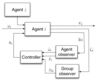
Figure 3: Control architecture for agent $\nu_{i}$

We replace the first item of Assumption 3 with that $(A_{i},C_{si})$, for all $i=1,2,\dots,n$ is observable.

Step I: redundant mode remove

We first write the state and output of $x_{i}$ and $\omega_{i}$ for each agent in the compact form

$$\left[\begin{array}[]{c}\dot{x}_{i}\\ \dot{\omega}_{i}\end{array}\right] =\left[\begin{array}[]{cc}A_{i}&0\\ 0&S_{i}\end{array}\right]\left[\begin{array}[]{c}x_{i}\\ \omega_{i}\end{array}\right]+\left[\begin{array}[]{c}B_{i}\\ 0\end{array}\right]u_{i},$$

$$y_{si} =\left[\begin{array}[]{cc}C_{si}&C_{wi}\end{array}\right]\left[\begin{array}[]{c}x_{i}\\ \omega_{i}\end{array}\right].$$

We can then construct a new state $\overline{x}_{i}=W_{i}\left[\begin{array}[]{c}x_{i}\\ \omega_{i}\end{array}\right]$ and perform the state transformation such that

$$\dot{\overline{x}}_{i} =\overline{A}_{i}\overline{x}_{i}+\overline{B}_{i}u_{i}=\left[\begin{array}[]{cc}A_{i}&\overline{A}_{i12}\\ 0&\overline{A}_{i22}\end{array}\right]\overline{x}_{i}+\left[\begin{array}[]{c}B_{i}\\ 0\end{array}\right]u_{i},$$

$$y_{si} =\overline{C}_{i}\overline{x}_{i}=\left[\begin{array}[]{cc}C_{si}&\overline{C}_{i12}\end{array}\right]\overline{x}_{i}.$$

Similar to Section 4.1, we can show that the pair $(\overline{A}_{i},\overline{C}_{i})$ is observable and the eigenvalues of $\overline{A}_{i22}$ are a subset of the eigenvalues of $S_{i}$, $i=1,2,\dots,n$.

Step II: agent observer

Based on the information of the individual output information $y_{si}$, the following individual observer for each agent $\nu_{i}$ is proposed

$$\dot{\widehat{\overline{x}}}_{i}=\overline{A}_{i}\widehat{\overline{x}}_{i}+\overline{B}_{i}u_{i}+K_{ai}\left(\overline{C}_{i}\widehat{\overline{x}}_{i}-y_{si}\right),$$ (29a)

$$[\widehat{x}_{i}^{\rm\tiny T},\widehat{\omega}_{i}^{\rm\tiny T}]^{\rm\tiny T}=W_{i}^{-1}\widehat{\overline{x}}_{i},~{}i=1,2,\dots,n,$$ (29b)

where $K_{ai}$ is chosen such that $\overline{A}_{i}+K_{ai}\overline{C}_{i}$ is Hurwitz stable, $i=1,2\ldots,n$.

Step III: group observer

We transform (3) into its canonical form. Define $\chi_{0}=T_{0}x_{0}\in\mathbb{R}^{pn_{0}}$, where

$$T_{0}=\left[\begin{array}[]{c}C_{0}\\ \vdots\\ C_{0}A_{0}^{n_{0}-1}\end{array}\right].$$

Therefore, it follows that

$$\dot{\chi}_{0} =(\mathcal{A}_{0}+\mathcal{L}_{0})\chi_{0},$$

$$y_{0} =\mathcal{C}_{0}\chi_{0},$$

where $\mathcal{A}_{0}=\begin{bmatrix}0&I_{p(n_{0}-1)}\\ 0&0\end{bmatrix}\in\mathbb{R}^{pn_{0}\times pn_{0}}$, $\mathcal{L}_{0}=\\ \left[\begin{array}[]{c}0\\ C_{0}A_{0}^{n_{0}}(T_{0}^{\rm\tiny T}T_{0})^{-1}T_{0}^{\rm\tiny T}\end{array}\right]$, $\mathcal{C}_{0}=\left[\begin{array}[]{cc}I_{p}&0\end{array}\right]\in\mathbb{R}^{p\times pn_{0}}$.

Then, based on the neighbor-based group output information $\zeta_{i}$, the distributed observer is proposed

$$\dot{\widehat{\chi}}_{0i}=~{}(\mathcal{A}_{0}+\mathcal{L}_{0})\widehat{\chi}_{0i} -S(\varepsilon)\mathcal{P}\mathcal{C}_{0}^{\rm\tiny T}\left(\sum_{j=0}^{n}a_{ij}(t)(y_{di}-y_{dj})\right.$$

$$\left.-\sum_{j=0}^{n}a_{ij}(t)(\widehat{y}_{i}-\widehat{y}_{j})\right),$$ (31a)

$$\widehat{x}_{0i}=(T_{0}^{\rm\tiny T}T_{0})^{-1}T_{0}^{\rm\tiny T}\widehat{\chi}_{0i},~{}~{}~{}i=1,2\ldots,n,$$ (31b)

where $a_{ij}(t)$, $i=0,1,\ldots,n$, $j=0,1,\ldots,n$, is entry $(i,j)$ of the adjacency matrix $\overline{{A}}_{\sigma(t)}$ associated with $\overline{{G}}_{\sigma(t)}$ defined in Section 2 at time $t$, the relative estimation information $\sum_{j=0}^{n}a_{ij}(t)(\widehat{y}_{i}-\widehat{y}_{j})$ is obtained using the communication infrastructure with $\widehat{y}_{i}=C_{di}\widehat{x}_{i}-\mathcal{C}_{0}\widehat{\chi}_{0i}$, $i=1,2,\dots,n$ and $\widehat{y}_{0}=0$. In addition, $S(\varepsilon)={\rm diag}(I_{p}\varepsilon^{-1},I_{p}\varepsilon^{-2},\dots,I_{p}\varepsilon^{-n_{0}})$, where $\varepsilon\in(0,1]$ is a positive constant, and $\mathcal{P}=\mathcal{P}^{\rm\tiny T}$ is a positive definite matrix satisfying

$$\mathcal{A}_{0}\mathcal{P}+\mathcal{P}\mathcal{A}_{0}^{\rm\tiny T}-2\theta\mathcal{P}\mathcal{C}_{0}^{\rm\tiny T}\mathcal{C}_{0}\mathcal{P}+I_{pn_{0}}=0,$$ (32)

and $\theta$ is a positive constant satisfying $\theta<\frac{1}{2}\min_{\overline{{G}}_{k}\in\overline{\mathbb{G}}_{c}}\\ \min\Re\{\lambda(L_{k})\}$.

Step IV: controller design

The observer-based controller is proposed as

$$u_{i}=F_{i}\widehat{x}_{i}+(\Gamma_{1i}-F_{i}\Pi_{1i})\widehat{\omega}_{i}+(\Gamma_{2i}-F_{i}\Pi_{2i})\widehat{x}_{0i},$$ (33)

where $\Pi_{1i}$, $\Gamma_{1i}$, $\Pi_{2i}$, and $\Gamma_{2i}$ are the solutions of the following regulator equations

$$\Pi_{1i}S_{i} =A_{i}\Pi_{1i}+B_{i}\Gamma_{1i},$$ (34a)

$$0 =D_{si}\Pi_{1i}+D_{wi},$$ (34b)

$$\Pi_{2i}A_{0} =A_{i}\Pi_{2i}+B_{i}\Gamma_{2i},$$ (34c)

$$0 =D_{si}\Pi_{2i}+D_{0},\quad i=1,2\dots,n,$$ (34d)

and $F_{i}$ is chosen such that $A_{i}+B_{i}F_{i}$ is Hurwitz.

Corollary 2.

Let Assumptions 1, 2, 3 (the first item is replaced by that $(A_{i},C_{si})$ is observable), and 4 hold and assume that $\kappa\geq\frac{\alpha+4\theta\lambda^{2}_{\max}(\mathcal{P})}{1-\alpha}$, where $\alpha\in(0,1)$, $\theta$ and $\mathcal{P}$ are given by (32). Also, let $\widehat{x}_{i}$ and $\widehat{\omega}_{i}$ be obtained in (29), and $\widehat{x}_{0i}$ be obtained in (31). Then, there exists $\varepsilon_{1}^{*}\in(0,1]$ such that, if $\varepsilon\in(0,\varepsilon_{1}^{*}]$, (33) ensures that $\lim_{t\rightarrow\infty}e_{i}(t)=0$, $i=1,2\ldots,n$, for the multi-agent system (1)-(4).

Proof 5.3.

The proof is straightforward following the similar analysis given in Lemmas 1 and 3.

5.2 Case II: $(A_{i},C_{di})$ is observable

In this section, we use $y_{si}$ to estimate $\omega_{i}$ and use $\zeta_{i}$ to estimate both $x_{i}$ and $x_{0}$. The control of each agent is supposed to have the structure shown in Fig. 4.

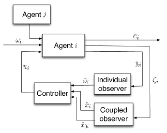
Figure 4: Control architecture for agent $\nu_{i}$

We also replace the first item of Assumption 3 with that $(A_{i},C_{di})$, for all $i=1,2,\dots,n$ is observable.

Step I: redundant mode remove

We first write the state and output of $x_{i}$ and $x_{0}$ for each agent in the compact form

$$\left[\begin{array}[]{c}\dot{x}_{i}\\ \dot{x}_{0}\end{array}\right]=\left[\begin{array}[]{cc}A_{i}&0\\ 0&A_{0}\end{array}\right]\left[\begin{array}[]{c}x_{i}\\ x_{0}\end{array}\right]+\left[\begin{array}[]{c}B_{i}\\ 0\end{array}\right]u_{i},$$

$$e_{di}=y_{di}-y_{d0}=\left[\begin{array}[]{cc}C_{di}&-C_{0}\end{array}\right]\left[\begin{array}[]{c}x_{i}\\ x_{0}\end{array}\right].$$

We can then construct a new state $\overline{x}_{i}=W_{i}\left[\begin{array}[]{c}x_{i}\\ x_{0}\end{array}\right]$ and perform the state transformation such that

$$\dot{\overline{x}}_{i}=\overline{A}_{i}\overline{x}_{i}+\overline{B}_{i}u_{i}=\left[\begin{array}[]{cc}A_{i}&\overline{A}_{i12}\\ 0&\overline{A}_{i22}\end{array}\right]\overline{x}_{i}+\left[\begin{array}[]{c}B_{i}\\ 0\end{array}\right]u_{i},$$

$$e_{di}=\overline{C}_{i}\overline{x}_{i}=\left[\begin{array}[]{cc}C_{di}&\overline{C}_{i12}\end{array}\right]\overline{x}_{i}.$$

Similarly, we can show that pair $(\overline{A}_{i},\overline{C}_{i})$ is observable and the eigenvalues of $\overline{A}_{i22}$ are a subset of the eigenvalues of $A_{0}$, $i=1,2,\dots,n$.

Step II: coupled observer

We next define $\chi_{i}=T_{i}\overline{x}_{i}\in\mathbb{R}^{p\overline{n}}$, $i=1,2,\dots,n$, where $\overline{n}=n_{0}+\max_{i=1,2,\dots,n}n_{i}$, and

$$T_{i}=\left[\begin{array}[]{c}\overline{C}_{i}\\ \vdots\\ \overline{C}_{i}\overline{A}_{i}^{\overline{n}-1}\end{array}\right].$$

Therefore, it follows that

$$\dot{\chi}_{i}=(\mathcal{A}+\mathcal{L}_{i})\chi_{i}+\mathcal{B}_{i}u_{i},$$ (37a)

$$e_{di}=\mathcal{C}\chi_{i},\quad i=1,2,\dots,n,$$ (37b)

where $\mathcal{A}=\left[\begin{array}[]{cc}0&I_{p(\overline{n}-1)}\\ 0&0\end{array}\right]\in\mathbb{R}^{p\overline{n}\times p\overline{n}}$, $\mathcal{L}_{i}=\left[\begin{array}[]{c}0\\ L_{i}\end{array}\right]$, $\mathcal{B}_{i}=T_{i}\overline{B}_{i}$, $\mathcal{C}=\left[\begin{array}[]{cc}I_{p}&0\end{array}\right]\in\mathbb{R}^{p\times p\overline{n}}$ for some matrix $L_{i}\in\mathbb{R}^{p\times p\overline{n}}$.

Based on the neighbor-based group output information $\zeta_{i}$, the distributed observer is proposed for (37) as

$$\dot{\widehat{\chi}}_{i}= (\mathcal{A}+\mathcal{L}_{i})\widehat{\chi}_{i}+\mathcal{B}_{i}u_{i}+S(\varepsilon)\mathcal{P}\mathcal{C}^{\rm\tiny T}$$

$$\times\left(\!\sum_{j=0}^{n}a_{ij}(t)(y_{di}-y_{dj})-\sum_{j=0}^{n}a_{ij}(t)(\widehat{y}_{i}-\widehat{y}_{j})\!\!\right),$$ (38a)

$$[\widehat{x}_{i}^{\rm\tiny T},\widehat{x}_{0i}^{\rm\tiny T}]^{\rm\tiny T}=W_{i}^{-1}(T_{i}^{\rm\tiny T}T_{i})^{-1}T_{i}^{\rm\tiny T}\widehat{\chi}_{i},~{}i=1,2,\dots,n,$$ (38b)

where $a_{ij}(t)$, $i=0,1,\ldots,n$, $j=0,1,\ldots,n$, is entry $(i,j)$ of the adjacency matrix $\overline{{A}}_{\sigma(t)}$ associated with $\overline{{G}}_{\sigma(t)}$ defined in Section 2 at time $t$, $\widehat{y}_{i}=\mathcal{C}\widehat{\chi}_{i}$, $i=1,2,\dots,n$, $\widehat{y}_{0}=0$. In addition, $S(\varepsilon)={\rm diag}(I_{p}\varepsilon^{-1},I_{p}\varepsilon^{-2},\dots,I_{p}\varepsilon^{-\overline{n}})$, where $\varepsilon\in(0,1]$ is a positive constant, and $\mathcal{P}=\mathcal{P}^{\rm\tiny T}$ is a positive definite matrix satisfying

$$\mathcal{A}\mathcal{P}+\mathcal{P}\mathcal{A}^{\rm\tiny T}-2\theta\mathcal{P}\mathcal{C}^{\rm\tiny T}\mathcal{C}\mathcal{P}+I_{p\overline{n}}=0,$$ (39)

where $\theta$ is a positive constant satisfying $\theta<\frac{1}{2}\min_{\overline{{G}}_{k}\in\overline{\mathbb{G}}_{c}}\\ \min\Re\{\lambda(L_{k})\}$.

Step III: individual observer

Based on the information of $\widehat{x}_{i}$ and the individual output information $y_{si}$, the following individual observer for each agent is proposed

$$\dot{\widehat{\omega}}_{i}=S_{i}\widehat{\omega}_{i}+K_{si}\left(C_{si}\widehat{x}_{i}+C_{wi}\widehat{\omega}_{i}-y_{si}\right),~{}i=1,2\ldots,n,$$ (40)

where $K_{si}$ is chosen such that $S_{i}+K_{si}C_{wi}$ is Hurwitz stable.

Step IV: controller design

The observer-based controller is proposed as

$$u_{i}=F_{i}\widehat{x}_{i}+(\Gamma_{1i}-F_{i}\Pi_{1i})\widehat{\omega}_{i}+(\Gamma_{2i}-F_{i}\Pi_{2i})\widehat{x}_{0i},$$ (41)

where $\Pi_{1i}$, $\Gamma_{1i}$, $\Pi_{2i}$, and $\Gamma_{2i}$ are the solutions of the following regulator equations

$$\Pi_{1i}S_{i} =A_{i}\Pi_{1i}+B_{i}\Gamma_{1i},$$ (42a)

$$0 =D_{si}\Pi_{1i}+D_{wi},$$ (42b)

$$\Pi_{2i}A_{0} =A_{i}\Pi_{2i}+B_{i}\Gamma_{2i},$$ (42c)

$$0 =D_{si}\Pi_{2i}+D_{0},\quad i=1,2\dots,n.$$ (42d)

and $F_{i}$ is chosen such that $A_{i}+B_{i}F_{i}$ is Hurwitz.

Corollary 3.

Let Assumptions 1, 2, 3 (the first item is replaced by that $(A_{i},C_{di})$ is observable), and 4 hold and assume that $\kappa\geq\frac{\alpha+4\theta\lambda^{2}_{\max}(\mathcal{P})}{1-\alpha}$, where $\alpha\in(0,1)$, $\theta$ and $\mathcal{P}$ are given by (39). Also, let $\widehat{x}_{i}$ and $\widehat{x}_{0i}$ be obtained in (38), and $\widehat{\omega}_{i}$ be obtained in (40). Then, there exists $\varepsilon_{2}^{*}\in(0,1]$ such that, if $\varepsilon\in(0,\varepsilon_{2}^{*}]$, (41) ensures that $\lim_{t\rightarrow\infty}e_{i}(t)=0$, $i=1,2\ldots,n$, for the multi-agent system (1)-(4).

Proof 5.4.

See [1].

6 Simulation Results

In this section, we illustrate the theoretical results. Consider a network of three agents as shown in Fig. 2. We assume that the adjacency matrix $\overline{{A}}_{\sigma(t)}$ associated with $\overline{{G}}_{\sigma(t)}$ is switching periodically. Denote $\ell=0,20,40\dots$.

$\overline{{A}}=\begin{cases}\left[\begin{matrix}0&0&0&0\\ 1&0&1&0\\ 0&1&0&0\\ 0&0&1&0\end{matrix}\right],&{\rm when}~{}~{}t\in[\ell,\ell+6),\\ \left[\begin{matrix}0&0&0&0\\ 1&0&0&0\\ 0&1&0&1\\ 0&0&1&0\end{matrix}\right],&{\rm when}~{}~{}t\in[\ell+6,\ell+12),\\ \left[\begin{matrix}0&0&0&0\\ 1&0&0&0\\ 0&1&0&0\\ 0&0&1&0\end{matrix}\right],&{\rm when}~{}~{}t\in[\ell+12,\ell+18),\\ \left[\begin{matrix}0&0&0&0\\ 0&0&0&0\\ 0&0&0&0\\ 0&0&0&0\end{matrix}\right],&{\rm when}~{}~{}t\in[\ell+18,\ell+20).\end{cases}$

Example 1

We give an example to validate Theorem 1, the dynamics of the agents are described as $A_{1}=\left[\begin{array}[]{ccc}0&3&0\\ 0&0&2\\ 0&-1&0\end{array}\right]$, $B_{1}=\left[\begin{array}[]{c}0\\ 0\\ 1\end{array}\right]$, $C_{s1}=C_{d1}=D_{s1}=\left[\begin{array}[]{ccc}1&1&1\end{array}\right]$, $A_{2}=\left[\begin{array}[]{cc}1&0\\ 0&0\end{array}\right]$, $B_{2}=\left[\begin{array}[]{cc}1\\ 1\end{array}\right]$, $C_{s2}=\left[\begin{array}[]{cc}1&0\end{array}\right]$, $C_{d2}=\left[\begin{array}[]{cc}0&1\end{array}\right]$, $D_{s2}=\left[\begin{array}[]{cc}1&1\end{array}\right]$, $A_{3}=\left[\begin{array}[]{cc}0&1\\ -2&-2\end{array}\right]$, $B_{3}=\left[\begin{array}[]{c}0\\ 1\end{array}\right]$, $C_{s3}=C_{d3}=D_{s3}=\left[\begin{array}[]{ccc}1&0\end{array}\right]$. The dynamics of the individual autonomous exosystems are described as $S_{i}=0$, $C_{wi}=D_{wi}=-1$, $i=1,2,3$, and $\omega_{1}(0)=-2$, $\omega_{2}(0)=-4$, and $\omega_{3}(0)=-6$. The dynamics of the group autonomous exosystem are described as $A_{0}=\left[\begin{array}[]{cc}0&1\\ -1&0\end{array}\right]$, $C_{0}=\left[\begin{array}[]{cc}1&0\end{array}\right]$, $D_{0}=-C_{0}$.

Following the design scheme proposed in Section 4, for the solutions of regulator equations (7), we have that $F_{1}=\left[\begin{array}[]{ccc}-1&-4.5&-6\end{array}\right]$, $\Pi_{1}=\left[\begin{array}[]{ccc}1&1.0345&-0.4138\\ 0&0.1379&0.3448\\ 0&-0.1724&0.0690\end{array}\right]$, $\Gamma_{1}=\left[\begin{array}[]{ccc}0&0.0690&0.1724\end{array}\right]$ for agent $\nu_{1}$, $F_{2}=\left[\begin{array}[]{cc}-2&-6\end{array}\right]$, $\Pi_{2}=\left[\begin{array}[]{ccc}0&0.4&-0.2\\ 1&0.6&0.2\end{array}\right]$, $\Gamma_{2}=\left[\begin{array}[]{ccc}0&-0.2&0.6\end{array}\right]$ for agent $\nu_{2}$, $F_{3}=\left[\begin{array}[]{cc}0&-1\end{array}\right]$, $\Pi_{3}=\left[\begin{array}[]{ccc}1&1&0\\ 0&0&1\end{array}\right]$, $\Gamma_{3}=\left[\begin{array}[]{ccc}2&1&2\end{array}\right]$ for agent $\nu_{3}$. We also have $\varepsilon=0.2$ for (14) and $\theta=0.1$ for (17).

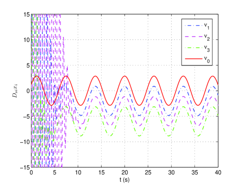
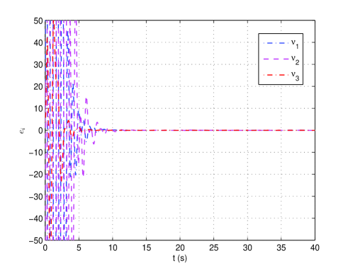
Figure 5: Output convergence of system (1), (2), and (3) under the observer-based controller (26) for Theorem 1

Figure 6: Error convergence of system (1), (2), and (3) under the observer-based controller (26) for Theorem 1

Figs. 6 and 6 show, respectively, the state convergence and the error convergence of system (1), (2), and (3) under the observer-based controller (26). We see that coordinated output regulation is realized even when there exists multiple heterogenous dynamics and the information interactions are switching. This agrees with Theorem 1.

Example 2

We next give an example to validate Corollary 2. In this section, the dynamics of the agents are described as $A_{1}=\left[\begin{array}[]{ccc}0&3&0\\ 0&0&2\\ 0&-1&0\end{array}\right]$, $B_{1}=\left[\begin{array}[]{c}0\\ 0\\ 1\end{array}\right]$, $C_{s1}=C_{d1}=D_{s1}=\left[\begin{array}[]{ccc}1&1&1\end{array}\right]$, $A_{2}=\left[\begin{array}[]{cc}0&1\\ 0&0\end{array}\right]$, $B_{2}=\left[\begin{array}[]{c}0\\ 1\end{array}\right]$, $C_{s2}=C_{d2}=D_{s2}=\left[\begin{array}[]{ccc}1&0\end{array}\right]$, $A_{3}=\left[\begin{array}[]{cc}0&1\\ -2&-2\end{array}\right]$, $B_{3}=\left[\begin{array}[]{c}0\\ 1\end{array}\right]$, $C_{s3}=C_{d3}=D_{s3}=\left[\begin{array}[]{ccc}1&0\end{array}\right]$. The dynamics of the individual autonomous exosystem are described as $\omega_{1}(t)=0$, $\omega_{2}(t)=0$, and $\omega_{3}(t)=0$. The dynamics of the group autonomous exosystem are described as $A_{0}=\left[\begin{array}[]{cc}0&1\\ -1&0\end{array}\right]$, $C_{0}=\left[\begin{array}[]{cc}1&0\end{array}\right]$, $D_{0}=-C_{0}$.

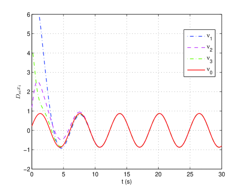
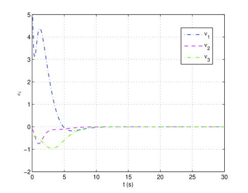
Figure 7: Output convergence of system (1), (2), and (3) under the observer-based controller (33) for Corollary 2

Figure 8: Error convergence of system (1), (2), and (3) under the observer-based controller (33) for Corollary 2

Following the design scheme proposed in Section 5.1, for the solutions of regulator equations (34), we have that $F_{1}=\left[\begin{array}[]{ccc}-1&-4.5&-6\end{array}\right]$, $\Pi_{21}=\left[\begin{array}[]{cc}1.0345&-0.4138\\ 0.1379&0.3448\\ -0.1724&0.0690\end{array}\right]$, $\Gamma_{21}=\left[\begin{array}[]{cc}0.0690&0.1724\end{array}\right]$ for agent $\nu_{1}$, $F_{2}=\left[\begin{array}[]{cc}-2&-3\end{array}\right]$, $\Pi_{22}=\left[\begin{array}[]{cc}1&0\\ 0&1\end{array}\right]$, $\Gamma_{22}=\left[\begin{array}[]{cc}-1&0\end{array}\right]$ for agent $\nu_{2}$, $F_{3}=\left[\begin{array}[]{cc}0&-1\end{array}\right]$, $\Pi_{23}=\left[\begin{array}[]{cc}1&0\\ 0&1\end{array}\right]$, $\Gamma_{23}=\left[\begin{array}[]{cc}1&2\end{array}\right]$ for agent $\nu_{3}$. We also have $K_{a1}=[-0.75,-4,-1.25]^{\rm\tiny T}$, $K_{a2}=[-3,-2]^{\rm\tiny T}$, $K_{a3}=[-1,2]^{\rm\tiny T}$ for (29), $\varepsilon=0.2$ for (31) and $\theta=0.1$ for (32).

Figs. 8 and 8 show, respectively, the state convergence and the error convergence of system (1), (2), and (3) under the observer-based controller (33). We see that coordinated output regulation is realized even when there exists multiple heterogenous dynamics and the information interactions are switching. This agrees with Corollary 2.

Example 3

We give an example to validate Corollary 3, the dynamics of the agents are described as $A_{1}=\left[\begin{array}[]{ccc}0&3&0\\ 0&0&2\\ 0&-1&0\end{array}\right]$, $B_{1}=\left[\begin{array}[]{c}0\\ 0\\ 1\end{array}\right]$, $C_{s1}=C_{d1}=D_{s1}=\left[\begin{array}[]{ccc}1&1&1\end{array}\right]$. $A_{2}=\left[\begin{array}[]{cc}0&1\\ 0&0\end{array}\right]$, $B_{2}=\left[\begin{array}[]{c}0\\ 1\end{array}\right]$, $C_{s2}=C_{d2}=D_{s2}=\left[\begin{array}[]{ccc}1&0\end{array}\right]$. $A_{3}=\left[\begin{array}[]{cc}0&1\\ -2&-2\end{array}\right]$, $B_{3}=\left[\begin{array}[]{c}0\\ 1\end{array}\right]$, $C_{s3}=C_{d3}=D_{s3}=\left[\begin{array}[]{ccc}1&0\end{array}\right]$. The dynamics of the individual autonomous exosystems are described as $S_{i}=0$, $C_{wi}=D_{wi}=-1$, $i=1,2,3$, and $\omega_{1}(0)=-2$, $\omega_{2}(0)=-4$, and $\omega_{3}(0)=-6$. The dynamics of the group autonomous exosystem are described as $A_{0}=\left[\begin{array}[]{cc}0&1\\ -1&0\end{array}\right]$, $C_{0}=\left[\begin{array}[]{cc}1&0\end{array}\right]$, $D_{0}=-C_{0}$.

Following the design scheme proposed in Section 5.2, for the solutions of regulator equations (42), we have that $F_{1}=\left[\begin{array}[]{ccc}-1&-4.5&-6\end{array}\right]$, $\Pi_{11}=\left[\begin{array}[]{c}1\\ 0\\ 0\end{array}\right]$, $\Gamma_{11}=0$, $\Pi_{21}=\left[\begin{array}[]{cc}1.0345&-0.4138\\ 0.1379&0.3448\\ -0.1724&0.0690\end{array}\right]$, $\Gamma_{21}=\left[\begin{array}[]{cc}0.0690&0.1724\end{array}\right]$ for agent $\nu_{1}$, $F_{2}=\left[\begin{array}[]{cc}-2&-3\end{array}\right]$, $\Pi_{12}=\left[\begin{array}[]{c}1\\ 0\end{array}\right]$, $\Gamma_{12}=0$, $\Pi_{22}=\left[\begin{array}[]{cc}1&0\\ 0&1\end{array}\right]$, $\Gamma_{22}=\left[\begin{array}[]{cc}-1&0\end{array}\right]$ for agent $\nu_{2}$, $F_{3}=\left[\begin{array}[]{cc}0&-1\end{array}\right]$, $\Pi_{13}=\left[\begin{array}[]{c}1\\ 0\end{array}\right]$, $\Gamma_{13}=-2$, $\Pi_{23}=\left[\begin{array}[]{cc}1&0\\ 0&1\end{array}\right]$, $\Gamma_{23}=\left[\begin{array}[]{cc}1&2\end{array}\right]$ for agent $\nu_{3}$. We also have $\varepsilon=0.2$ for (38), $\theta=0.1$ for (39), and $K_{si}=1$, $i=1,2,3$ for (40),

Figs. 10 and 10 show, respectively, the state convergence and the error convergence of system (1), (2), and (3) under the observer-based controller (41). We see that coordinated output regulation is realized even when there exists multiple heterogenous dynamics and the information interactions are switching. This agrees with Corollary 3.

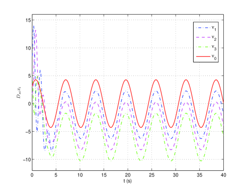
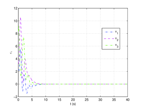
Figure 9: Output convergence of system (1), (2), and (3) under the observer-based controller (41) for Corollary 3

Figure 10: Error convergence of system (1), (2), and (3) under the observer-based controller (41) for Corollary 3

7 Conclusions

This paper studied the coordinated output regulation problem of multiple heterogeneous linear systems. We first formulated the coordinated output regulation problem and specified the information that is available for each agent. A high-gain based distributed observer and an individual observer were introduced for each agent and observer-based controllers were designed to solve the problem. The information interactions among the agents and the group autonomous exosystem were allowed to be switching over a finite set of fixed networks containing both the graph having a spanning tree and the graph having not. The relationship of the information interactions, the dwell time, the non-identical dynamics of different agents, and the high-gain parameters were also given. Simulations were given to validate the theoretical results. Future directions include relaxing the dwell-time assumption.

References

- [1] Z. Meng, T. Yang, D. V. Dimarogonas, K. H. Johansson, Coordinated output regulation of multiple heterogeneous linear systems, in: 52th IEEE Conference on Decision and Control, Florence, Italy, 2013, pp. 2175–2180.
- [2] J. Cortes, S. Martinez, F. Bullo, Robust rendezvous for mobile autonomous agents via proximity graphs in arbitrary dimensions, IEEE Transactions on Automatic Control 51 (8) (2006) 1289–1298.
- [3] H. G. Tanner, A. Jadbabaie, G. J. Pappas, Flocking in fixed and switching networks, IEEE Transactions on Automatic Control 52 (5) (2007) 863–868.
- [4] N. Chopra, M. W. Spong, On exponential synchronization of kuramoto oscillators, IEEE Transactions on Automatic Control 54 (2) (2009) 353–357.
- [5] H. Bai, M. Arcak, J. Wen, Cooperative control design: A systematic, passivity-based approach, Communications and Control Engineering, Springer, New York, 2011.
- [6] A. Jadbabaie, J. Lin, A. S. Morse, Coordination of groups of mobile autonomous agents using nearest neighbor rules, IEEE Transactions on Automatic Control 48 (6) (2003) 988–1001.
- [7] R. Olfati-Saber, J. A. Fax, R. M. Murray, Consensus and cooperation in networked multi-agent systems, Proceedings of the IEEE 95 (1) (2007) 215–233.
- [8] V. D. Blondel, J. M. Hendrickx, A. Olshevsky, J. N. Tsitsiklis, Convergence in multiagent coordination, consensus, and flocking, in: 44th IEEE Conference on Decision and Control, 2005, pp. 2996–3000.
- [9] W. Ren, R. W. Beard, Consensus seeking in multiagent systems under dynamically changing interaction topologies, IEEE Transactions on Automatic Control 50 (5) (2005) 655–661.
- [10] L. Moreau, Stability of multi-agent systems with time-dependent communication links, IEEE Transactions on Automatic Control 50 (2) (2005) 169–182.
- [11] K. You, L. Xie, Network topology and communication data rate for consensusability of discrete-time multi-agent systems, IEEE Transactions on Automatic Control 56 (10) (2011) 2262–2275.
- [12] Z. Lin, B. Francis, M. Maggiore, State agreement for continuous-time coupled nonlinear systems, SIAM Journal of Control and Optimization 46 (1) (2007) 288–307.
- [13] M. Cao, A. S. Morse, B. D. O. Anderson, Reaching a consensus in a dynamically changing environment: convergence rates, measurement delays, and asynchronous events, SIAM Journal of Control and Optimization 47 (2) (2008) 601–623.
- [14] K. Cai, H. Ishii, Quantized consensus and averaging on gossip digraphs, IEEE Transactions on Automatic Control 56 (9) (2011) 2087–2100.
- [15] G. Shi, Y. Hong, K. H. Johansson, Connectivity and set tracking of multi-agent systems guided by multiple moving leaders, IEEE Transactions on Automatic Control 57 (3) (2012) 663–676.
- [16] P. Wieland, J.-S. Kim, F. Allgöwer, On topology and dynamics of consensus among linear high-order agents, International Journal of Systems Science 42 (10) (2011) 1831–1842.
- [17] S. E. Tuna, Conditions for synchronizability in arrays of coupled linear systems, IEEE Transactions on Automatic Control 54 (10) (2009) 2416–2420.
- [18] L. Scardovi, R. Sepulchre, Synchronization in networks of identical linear systems, Automatica 45 (11) (2009) 2557–2562.
- [19] J. Wang, D. Cheng, X. Hu, Consensus of multi-agent linear dynamic systems, Asian Journal of Control 10 (2) (2008) 144–155.
- [20] W. Ni, D. Cheng, Leader-following consensus of multi-agent systems under fixed and switching topologies, Systems and Control Letters 59 (3-4) (2010) 209–217.
- [21] Z. Li, Z. Duan, G. Chen, L. Huang, Consensus of multiagent systems and synchronization of complex networks: A unified viewpoint, IEEE Transactions on Circuits and Systems - I: Regular Papers 57 (1) (2010) 213–224.
- [22] J. H. Seo, H. Shim, J. Back, Consensus of high-order linear systems using dynamic output feedback compensator: low gain approach, Automatica 45 (11) (2009) 2659–2664.
- [23] T. Yang, S. Roy, Y. Wan, A. Saberi, Constructing consensus controllers for networks with identical general linear agents, International Journal of Robust and Nonlinear Control 21 (11) (2011) 1237–1256.
- [24] J. Lunze, Synchronization of heterogeneous agents, IEEE Transactions on Automatic Control 57 (11) (2012) 2885–2890.
- [25] L. Alvergue, A. Pandey, G. Gu, X. Chen, Output consensus control for heterogeneous multi-agent systems, in: 52nd IEEE Conference on Decision and Control, Florence, Italy, 2013, pp. 1502–1507.
- [26] P. Wieland, R. Sepulchre, F. Allgöwer, An internal model principle is necessary and sufficient for linear output synchronization, Automatica 47 (5) (2011) 1068–1074.
- [27] H. F. Grip, T. Yang, A. Saberi, A. A. Stoorvogel, Output synchronization for heterogeneous networks of non-introspective agents, Automatica 48 (10) (2012) 2444–2453.
- [28] T. Yang, A. A. Stoorvogel, H. F. Grip, A. Saberi, Semi-global regulation of output synchronization for heterogeneous networks of non-introspective, invertible agents subject to actuator saturation, International Journal of Robust and Nonlinear Control 24 (3) (2014) 548–566.
- [29] D. Vengertsev, H. Kim, H. Shim, J. H. Seo, Consensus of output-coupled linear multi-agent systems under frequently connected network, in: 49th IEEE Conference on Decision and Control, Hilton Atlanta Hotel, Atlanta, GA, USA, 2010, pp. 4559–4564.
- [30] H. Kim, H. Shim, J. Back, J. H. Seo, Consensus of output-coupled linear multi-agent systems under fast switching network: Averaging approach, Automatica 49 (1) (2013) 267–272.
- [31] X. Wang, Y. Hong, J. Huang, Z. Jiang, A distributed control approach to a robust output regulation problem for multi-agent linear systems, IEEE Transactions on Automatic Control 55 (12) (2012) 2891–2895.
- [32] Y. Su, J. Huang, Cooperative output regulation of linear multi-agent systems, IEEE Transactions on Automatic Control 57 (4) (2012) 1062–1066.
- [33] Z. Ding, Consensus output regulation of a class of heterogeneous nonlinear systems, IEEE Transactions on Automatic Control 58 (10) (2013) 2648–2653.
- [34] J. Cao, Z. Wang, Y. Sun, Synchronization in an array of linearly stochastically coupled networks with time, Physica A: Statistical Mechanics and its Applications 385 (2) (2007) 718–728.
- [35] J. Cao, G. Chen, P. Li, Global synchronization in an array of delayed neural networks with hybrid coupling, IEEE Transactions on Systems, Man, and Cybernetics - Part B: Cybernetics 38 (2) (2008) 488–498.
- [36] G. Wang, J. Cao, J. Lu, Outer synchronization between two nonidentical networks with circumstance noise, Physica A: Statistical Mechanics and its Applications 389 (7) (2010) 1480–1488.
- [37] W. He, W. Du, F. Qian, J. Cao, Synchronization analysis of heterogeneous dynamical networks, Neurocomputing 104 (15) (2013) 146–154.
- [38] D. Liberzon, A. S. Morse, Basic problems in stability and design of switched systems, IEEE Control Systems Magazine 19 (5) (1999) 59–70.
- [39] A. Saberi, A. A. Stoorvogel, P. Sannuti, Control of linear systems with regulation and input constraints, Communications and Control Engineering. London, UK: Springer, 2003.
- [40] B. A. Francis, The linear multivariable regulator problem, SIAM Journal of Control and Optimization 15 (3) (1977) 486–505.
- [41] Z. Qu, Cooperative control of dynamical systems: applications to autonomous vehicles, Springer, 2009.
- [42] W. Ren, Y. Cao, Distributed Coordination of Multi-agent Networks: Emergent Problems, Models, and Issues, Springer, 2011.
- [43] G. Zhai, B. Hu, K. Yasuda, A. N. Michel, Piecewise Lyapunov functions for switched systems with average dwell time, Asian Journal of Control 2 (3) (2000) 192–197.