On Perturbed Proximal Gradient Algorithms

Abstract

We study a version of the proximal gradient algorithm for which the gradient is intractable and is approximated by Monte Carlo methods (and in particular Markov Chain Monte Carlo). We derive conditions on the step size and the Monte Carlo batch size under which convergence is guaranteed: both increasing batch size and constant batch size are considered. We also derive non-asymptotic bounds for an averaged version. Our results cover both the cases of biased and unbiased Monte Carlo approximation. To support our findings, we discuss the inference of a sparse generalized linear model with random effect and the problem of learning the edge structure and parameters of sparse undirected graphical models.

Keywords: Proximal Gradient Methods; Stochastic Optimization; Monte Carlo approximations; Perturbed Majorization-Minimization algorithms.

1 Introduction

This paper deals with statistical optimization problems of the form:

$$\text{{(P)}}\quad\min_{\theta\in\mathbb{R}^{d}}F(\theta)\qquad\text{with $F=f+g$}\;.$$

This problem occurs in a variety of statistical and machine learning problems, where $f$ is a measure of fit depending implicitly on some observed data and $g$ is a regularization term that imposes structure to the solution. Typically, $f$ is a differentiable function with a Lipschitz gradient, whereas $g$ might be non-smooth (typical examples include sparsity inducing penalty).

H 1.

The function $g:\;\mathbb{R}^{d}\to\left[0,+\infty\right]$ is convex, not identically $+\infty$, and lower semi-continuous. The function $f:\mathbb{R}^{d}\to\mathbb{R}$ is convex, continuously differentiable on $\mathbb{R}^{d}$ and there exists a finite non-negative constant $L$ such that, for all $\theta,\theta^{\prime}\in\mathbb{R}^{d}$,

$$\|\nabla f(\theta)-\nabla f(\theta^{\prime})\|\leq L\|\theta-\theta^{\prime}\|\;,$$

where $\nabla f$ denotes the gradient of $f$.

We denote by $\Theta$ the domain of $g$: $\Theta\stackrel{{\scriptstyle\mathrm{def}}}{{=}}\{\theta\in\mathbb{R}^{d}:g(\theta)<\infty\}$.

H 2.

The set $\mathrm{argmin}_{\theta\in\Theta}F(\theta)$ is a non empty subset of $\Theta$.

In this paper, we focus on the case where $f+g$ and $\nabla f$ are both intractable. This setting has not been widely considered despite the considerable importance of such models in statistics and machine learning. Intractable likelihood problems naturally occur for example in inference for bayesian networks (e.g. learning the edge structure and the parameters in an undirected graphical models), regression with latent variables or random effets, missing data, etc… In such applications, $f$ is the negated log-likelihood of a conditional Gibbs measure $\pi_{\theta}$ known only up to a normalization constant and the gradient of $\nabla f(\theta)$ is typically expressed as a very high-dimensional integral w.r.t. the associated Gibbs measure $\nabla f(\theta)=\int H_{\theta}(x)\pi_{\theta}(\mathrm{d}x)$. Of course, this integral cannot be computed in closed form and should be approximated. Most often, some forms of Monte Carlo integration (such as Markov Chain Monte Carlo, or MCMC) is the only option.

To cope with problems where $f+g$ is intractable and possibly non-smooth, various methods have been proposed. Some of these works focused on stochastic sub-gradient and mirror descent algorithms; see Nemirovski et al. (2008); Duchi et al. (2011); Cotter et al. (2011); Lan (2012); Juditsky and Nemirovski (2012a, b). Other authors have proposed algorithms based on proximal operators to better exploit the smoothness of $f$ and the properties of $g$ (see e.g. Combettes and Wajs (2005); Hu et al. (2009); Xiao (2010); Juditsky and Nemirovski (2012a, b)).

The current paper focuses on the proximal gradient algorithm (see e.g. Beck and Teboulle (2010); Combettes and Pesquet (2011); Parikh and Boyd (2013) for literature review and further references). The proximal map (Moreau (1962)) associated to $g$ is defined for $\gamma>0$ and $\theta\in\mathbb{R}^{d}$ by:

$$\operatorname{Prox}_{\gamma,g}(\theta)\stackrel{{\scriptstyle\mathrm{def}}}{{=}}\operatorname{argmin}_{\vartheta\in\Theta}\left\{g(\vartheta)+\frac{1}{2\gamma}\|\vartheta-\theta\|^{2}\right\}.$$ (1)

Note that under H 1, there exists an unique point $\vartheta$ minimizing the RHS of (1) for any $\theta\in\mathbb{R}^{d}$ and $\gamma>0$. The proximal gradient algorithm is an iterative algorithm which, given an initial value $\theta_{0}\in\Theta$ and a sequence of positive step sizes $\{\gamma_{n},n\in{\mathbb{N}}\}$, produces a sequence of parameters $\{\theta_{n},n\in{\mathbb{N}}\}$ as follows:

Algorithm 1 (Proximal gradient algorithm).

Given $\theta_{n}$, compute

$$\theta_{n+1}=\operatorname{Prox}_{\gamma_{n+1},g}\left(\theta_{n}-\gamma_{n+1}\nabla f(\theta_{n})\right)\;.$$ (2)

When $\gamma_{n}=\gamma$ for any $n$, it is known that the iterates of the proximal gradient algorithm $\{\theta_{n},n\in{\mathbb{N}}\}$ (Algorithm 1) converges to $\theta_{\infty}$, this point is a fixed point of the proximal-gradient map

$$T_{\gamma}(\theta)\stackrel{{\scriptstyle\mathrm{def}}}{{=}}\operatorname{Prox}_{\gamma,g}\left(\theta-\gamma\nabla f(\theta)\right)\;.$$ (3)

Under H 1 and H 2, when $\gamma_{n}\left(0,2/L\right]$ and $\inf_{n}\gamma_{n}>0$, it is indeed known that the iterates of the proximal gradient algorithm $\{\theta_{n},\;n\in{\mathbb{N}}\}$ defined in (2) converges to a point in the set $\mathcal{L}$ of the solutions of $(P)$ which coincides with the fixed points of the mapping $T_{\gamma}$ for any $\gamma\in\left(0,2/L\right)$

$$\mathcal{L}\stackrel{{\scriptstyle\mathrm{def}}}{{=}}\operatorname{argmin}_{\theta\in\Theta}F(\theta)=\{\theta\in\Theta:\theta=T_{\gamma}(\theta)\}\;.$$ (4)

(see e.g. (Combettes and Wajs, 2005, Theorem 3.4. and Proposition 3.1.(iii))).

Since $\nabla f(\theta)$ is intractable, the gradient $\nabla f(\theta_{n})$ at $n$-th iteration is replaced by an approximation $H_{n+1}$:

Algorithm 2 (Perturbed Proximal Gradient algorithm).

Let $\theta_{0}\in\Theta$ be the initial solution and $\{\gamma_{n},\;n\in{\mathbb{N}}\}$ be a sequence of positive step sizes. For $n\geq 1$, given $(\theta_{0},\dots,\theta_{n})$ construct an approximation $H_{n+1}$ of $\nabla f(\theta_{n})$ and compute

$$\theta_{n+1}=\operatorname{Prox}_{\gamma_{n+1},g}\left(\theta_{n}-\gamma_{n+1}H_{n+1}\right)\;.$$ (5)

We provide in Theorem 1 sufficient conditions on the perturbation $\eta_{n+1}=H_{n+1}-\nabla f(\theta_{n})$ to obtain the convergence of the perturbed proximal gradient sequence given by (5). We then consider an averaging scheme of the perturbed proximal gradient algorithm: given non-negative weights $\{a_{n},\;n\in{\mathbb{N}}\}$, Theorem 2 provides non-asymptotic bound of the deviation between $\sum_{k=1}^{n}a_{k}F(\theta_{k})/\sum_{k=1}^{n}a_{k}$ and the minimum of $F$. Our results complement and extend Rosasco et al. (2014); Nitanda (2014); Xiao and Zhang (2014).

We then consider the case where the gradient $\nabla f(\theta)=\int_{\mathsf{X}}H_{\theta}(x)\pi_{\theta}(\mathrm{d}x)$ is defined as an expectation (see H 3 in section 3). In this case, at each iteration $\nabla f(\theta_{n})$ is approximated by a Monte Carlo average $H_{n+1}=m_{n+1}^{-1}\sum_{j=1}^{m_{n+1}}H_{\theta_{n}}(X_{n+1}^{(j)})$ where $m_{n+1}$ is the size of the Monte Carlo batch and $\{X_{n+1}^{(j)},1\leq j\leq m_{n+1}\}$ is the Monte Carlo batch. Two different settings are covered. In the first setting, the samples $\{X_{n+1}^{(j)},1\leq j\leq m_{n+1}\}$ are conditionally independent and identically distributed (i.i.d.) with distribution $\pi_{\theta_{n}}$. In such case, the conditional expectation of $H_{n+1}$ given all the past iterations, denoted by ${\mathbb{E}}\left[\left.H_{n+1}\,\right|\mathcal{F}_{n}\right]$ (see section 3), is equal to $\nabla f(\theta_{n})$. In the second setting, the Monte Carlo batch $\{X_{n+1}^{(j)},1\leq j\leq m_{n+1}\}$ is produced by running a MCMC algorithm. In such case, the conditional distribution of $X_{n+1}^{(j)}$ given the past is no longer exactly equal to $\pi_{\theta_{n}}$ which implies that ${\mathbb{E}}\left[\left.H_{n+1}\,\right|\mathcal{F}_{n}\right]\neq\nabla f(\theta_{n})$.

Theorem 3 (resp. Theorem 4) establish the convergence of the sequence $\{\theta_{n},n\in{\mathbb{N}}\}$ when the batch size $m_{n}$ is either fixed or increases with the number of iterations $n$. When the Monte Carlo batch $\{X_{n+1}^{(j)},1\leq j\leq m_{n+1}\}$ is i.i.d. conditionally to the past the two theorems essentially say that with probability one, $\{\theta_{n},n\in{\mathbb{N}}\}$ converges to an element of the set of minimizer $\mathcal{L}$ as soon as $\sum_{n}\gamma_{n}=+\infty$ and $\sum_{n}\gamma_{n+1}^{2}/m_{n+1}<\infty$. Hence, one can choose either a fixed step size $\gamma_{n}=\gamma$ and a batch size $\{m_{n},n\in{\mathbb{N}}\}$ increasing at least linearly (up to a logarithmic factor); or a decreasing step size and a fixed batch size $m_{n}=m$. When $\{X_{n+1}^{(j)},1\leq j\leq m_{n+1}\}$ is produced by a MCMC algorithm (under appropriate assumptions) our theorems essentially say that the same convergence result holds if $\sum_{n}\gamma_{n}=\infty$ and $\sum_{n}\gamma_{n+1}^{2}<\infty$ when $m_{n}=m$ is constant across iterations or $\sum_{n}\gamma_{n+1}/m_{n+1}<\infty$ if the batch size is increased.

Theorem 3 and Theorem 4 also provide non asymptotic bounds for the difference $\Delta_{n}=\sum_{k=1}^{n}a_{k}F(\theta_{k})/\sum_{k=1}^{n}a_{k}-\min F$ in $L^{q}$-norm for $q\geq 1$. When the batch size sequence $m_{n+1}$ increases linearly at each iteration while the step size $\gamma_{n+1}$ is held constant, $\Delta_{n}=O(\ln n/n)$. We recover (up to a logarithmic factor) the rate of the proximal gradient algorithm. If we now compare the complexity of the algorithms in terms of the number of simulations $N$ needed (and not the number of iterations), the error bound decreases like $O(N^{-1/2})$. The same error bound can be achieved by choosing a fixed batch size and a decreasing step size $\gamma_{n}=O(1/\sqrt{n})$.

In section 4, these results are illustrated with the problem of estimating a high-dimensional discrete graphical models. In section 5, we consider high-dimensional random effect logistic regression model. All the proofs are postponed to section 6.

2 Perturbed proximal gradient algorithms

The key property to study the behavior of the sequence the perturbed proximal gradient algorithm is the following elementary lemma which might be seen as a deterministic version of the Robbins-Siegmund lemma (see e.g. (Polyak, 1987, Lemma 11, Chapter 2)). It replaces in our analysis (Combettes, 2001, Lemma 3.1) for quasi-Fejer sequences and modified Fejer monotone sequences (see Lin et al. (2015)). Compared to the Robbins-Siegmund Lemma, the sequence $(\xi_{n})_{n}$ is not assumed to be nonnegative. When applied in the stochastic context as in Section 3, the fact that the result is purely deterministic and deals with signed perturbations $\xi_{n}$ allows more flexibility in the study of the dynamics.

Lemma .

Let $\{v_{n},\;n\in{\mathbb{N}}\}$ and $\{\chi_{n},\;n\in{\mathbb{N}}\}$ be non-negative sequences and $\{\xi_{n},\;n\in{\mathbb{N}}\}$ be such that $\sum_{n}\xi_{n}$ exists. If for any $n\geq 0$,

$$v_{n+1}\leq v_{n}-\chi_{n+1}+\xi_{n+1}$$

then $\sum_{n}\chi_{n}<\infty$ and $\lim_{n}v_{n}$ exists.

Proof.

See Section 6.2.1

Applied with $v_{n}=\|\theta_{n}-\theta_{\star}\|$ for some $\theta_{\star}\in\mathcal{L}$, this lemma is the key result for the proof of the following theorem, which provides sufficient conditions on the stepsize sequence $\{\gamma_{n},\;n\in{\mathbb{N}}\}$ and on the approximation error:

$$\eta_{n+1}\stackrel{{\scriptstyle\mathrm{def}}}{{=}}H_{n+1}-\nabla f(\theta_{n})\;,$$ (6)

for the sequence $\{\theta_{n},\;n\in{\mathbb{N}}\}$ to converge to a point $\theta_{\infty}$ in the set $\mathcal{L}$ of the minimizers of $F$. Denote by $\left\langle\cdot,\cdot\right\rangle$ the usual inner product on $\mathbb{R}^{d}$ associated to the norm $\|\cdot\|$.

Theorem 1.

Assume H 1 and H 2. Let $\{\theta_{n},\;n\in{\mathbb{N}}\}$ be given by Algorithm 2 with step sizes satisfying $\gamma_{n}\in\left(0,1/L\right]$ for any $n\geq 1$ and $\sum_{n}\gamma_{n}=+\infty$. If the following series converge

$$\sum_{n\geq 0}\gamma_{n+1}\left\langle T_{\gamma_{n+1}}(\theta_{n}),\eta_{n+1}\right\rangle\;,\,\quad\sum_{n\geq 0}\gamma_{n+1}\eta_{n+1}\;,\quad\sum_{n\geq 0}\gamma_{n+1}^{2}\|\eta_{n+1}\|^{2}\;,$$ (7)

then there exists $\theta_{\infty}\in\mathcal{L}$ such that $\lim_{n}\theta_{n}=\theta_{\infty}$.

Proof.

See Section 6.2.2.

Theorem 1 applied with $\eta_{n+1}=0$ provides sufficient conditions for the convergence of Algorithm 1 to $\mathcal{L}$: the algorithm converges as soon as $\gamma_{n}\in\left(0,1/L\right]$ and $\sum_{n}\gamma_{n}=+\infty$.

Sufficient conditions for the convergence of $\{\theta_{n},\;n\in{\mathbb{N}}\}$ are also provided in Combettes and Wajs (2005). When applied to our settings, Theorem 3.4. in Combettes and Wajs (2005) require $\sum_{n}\|\eta_{n+1}\|<\infty$ and $\inf_{n}\gamma_{n}>0$, which for instance cannot accommodate the fixed Monte Carlo batch size stochastic algorithms considered in this paper. The same limitation applies to the analysis of the stochastic quasi-Fejer iterations (see Combettes and Pesquet (2015a)) which in our particular case requires $\sum_{n}\gamma_{n+1}\|\eta_{n+1}\|<\infty$. These conditions are weakened in Theorem 1. However in all fairness we should mention that unlike the present work, Combettes and Wajs (2005) and Combettes and Pesquet (2015a) deal with infinite-dimensional problems which raises additional technical difficulties, and study algorithms that include a relaxation parameter. Furthermore, in the case where $\eta_{n}\equiv 0$, larger values of the stepsize $\gamma_{n}$ are allowed ($\gamma_{n}\in(0,2/L]$.)

Let $\{a_{0},\cdots,a_{n}\}$ be non-negative real numbers. Theorem 2 provides a control of the weighted sum $\sum_{k=1}^{n}a_{k}(F(\theta_{k})-\min F)$.

Theorem 2.

Assume H 1 and H 2. Let $\{\theta_{n},\;n\in{\mathbb{N}}\}$ be given by Algorithm 2 with $\gamma_{n}\in\left(0,1/L\right]$ for any $n\geq 1$. For any non-negative weights $\{a_{0},\cdots,a_{n}\}$, any $\theta_{\star}\in\mathcal{L}$ and any $n\geq 1$,

$$\sum_{k=1}^{n}a_{k}\left\{F(\theta_{k})-\min F\right\}\leq U_{n}(\theta_{\star})$$

where $T_{\gamma}$ and $\eta_{n}$ are given by (3) and (6) respectively and

$$U_{n}(\theta_{\star})\stackrel{{\scriptstyle\mathrm{def}}}{{=}}\frac{1}{2}\sum_{k=1}^{n}\left(\frac{a_{k}}{\gamma_{k}}-\frac{a_{k-1}}{\gamma_{k-1}}\right)\|\theta_{k-1}-\theta_{\star}\|^{2}+\frac{a_{0}}{2\gamma_{0}}\|\theta_{0}-\theta_{\star}\|^{2}\\ -\sum_{k=1}^{n}a_{k}\left\langle T_{\gamma_{k}}(\theta_{k-1})-\theta_{\star},\eta_{k}\right\rangle+\sum_{k=1}^{n}a_{k}\gamma_{k}\|\eta_{k}\|^{2}\;.$$ (8)

Proof.

See Section 6.2.3.

When applied with $\eta_{n}=0$, Theorem 2 gives an explicit bound of the difference $\Delta_{n}=A_{n}^{-1}\sum_{j=1}^{n}a_{j}F(\theta_{j})-\min F$ where $A_{n}=\sum_{k=1}^{n}a_{k}$ for the (exact) proximal gradient sequence $\{\theta_{n},\;n\in{\mathbb{N}}\}$ given by Algorithm 1. When the sequence $\{a_{n}/\gamma_{n},n\geq 1\}$ is non decreasing, (8) shows that $\Delta_{n}=O(a_{n}A_{n}^{-1}\gamma_{n}^{-1})$.

Taking $a_{k}=1$ for any $k\geq 0$ provides a bound for the cumulative regret. When $a_{k}=1$, $\gamma_{k}=1/L$ for any $k\geq 0$, (Schmidt et al., 2011, Proposition 1) provides a bound of order $O(1)$ under the assumption that $\sum_{n}\|\eta_{n+1}\|<\infty$. Using the inequality $|\left\langle T_{1/L}(\theta_{k})-\theta_{\star},\eta_{k+1}\right\rangle|\leq\|\theta_{k}-\theta_{\star}\|\|\eta_{k+1}\|$ (see Section 6.1), the upper bound $U_{n}(\theta_{\star})$ in (8) is also $O(1)$.

When $a_{n}=\gamma_{n}$ for any $n\geq 0$, then $\sup_{n}U_{n}(\theta_{\star})<\infty$ under the assumptions that the series

$$\sum_{n}\gamma_{n}\left\langle T_{\gamma_{n}}(\theta_{n-1})-\theta_{\star},\eta_{n}\right\rangle\;,\qquad\sum_{n}\gamma_{n}^{2}\|\eta_{n}\|^{2}\;,$$

converge. In this case, we have

$$\left(\frac{\sum_{k=1}^{n}\gamma_{k}F(\theta_{k})}{\sum_{k=1}^{n}\gamma_{k}}-\min F\right)=O\left(\left(\sum_{k=1}^{n}\gamma_{k}\right)^{-1}\right).$$

Consider the weighted averaged sequence $\{\bar{\theta}_{n},\;n\in{\mathbb{N}}\}$ defined by

$$\bar{\theta}_{n}\stackrel{{\scriptstyle\mathrm{def}}}{{=}}\frac{1}{A_{n}}\sum_{k=1}^{n}a_{k}\theta_{k}\;.$$ (9)

Under H 1 and H 2, $F$ is convex so that $F\left(\bar{\theta}_{n}\right)\leq A_{n}^{-1}\sum_{k=1}^{n}a_{k}F(\theta_{k})$. Therefore, Theorem 2 also provides convergence rates for $F(\bar{\theta}_{n})-\min F$.

3 Stochastic Proximal Gradient algorithm

In this section, it is assumed that $H_{n+1}$ is a Monte Carlo approximation of $\nabla f(\theta_{n})$, where $\nabla f(\theta)$ satisfies the following assumption:

H 3.

for all $\theta\in\Theta$,

$$\nabla f(\theta)=\int_{\mathsf{X}}H_{\theta}(x)\pi_{\theta}(\mathrm{d}x)\;,$$ (10)

for some probability measure $\pi_{\theta}$ on a measurable space $(\mathsf{X},\mathcal{X})$ and an integrable function $(\theta,x)\mapsto H_{\theta}(x)$ from $\Theta\times\mathsf{X}$ to $\Theta$.

Note that $\mathsf{X}$ is not necessarily a topological space, even if, in many applications, $\mathsf{X}\subseteq\mathbb{R}^{d}$.

Assumption H 3 holds in many problems (see section 4 and section 5). To approximate $\nabla f(\theta)$, several options are available. Of course, when the dimension of the state space $\mathsf{X}$ is small to moderate, it is always possible to perform a numerical integration using either Gaussian quadratures or low-discrepancy sequences. Another possibility is to approximate these integrals: nested Laplace approximations have been considered recently for example in Schelldorfer et al. (2014) and further developed in Ogden (2015). Such approximations necessarily introduce some bias, which might be difficult to control. In addition, these techniques are not applicable when the dimension of the state space $\mathsf{X}$ becomes large. In this paper, we rather consider some form of Monte Carlo approximation.

When sampling $\pi_{\theta}$ is doable, then an obvious choice is to use a naive Monte Carlo estimator which amounts to sample a batch $\{X_{n+1}^{(j)},1\leq j\leq m_{n+1}\}$ independently of the past values of the parameters $\{\theta_{j},j\leq n\}$ and of the past draws i.e. independently of the $\sigma$-algebra

$$\mathcal{F}_{n}\stackrel{{\scriptstyle\mathrm{def}}}{{=}}\sigma(\theta_{0},X_{k}^{(j)},0\leq k\leq n,0\leq j\leq m_{k})\;.$$ (11)

We then form

$$H_{n+1}=m_{n+1}^{-1}\sum_{j=1}^{m_{n+1}}H_{\theta_{n}}(X_{n+1}^{(j)})\;.$$

Conditionally to $\mathcal{F}_{n}$, $H_{n+1}$ is an unbiased estimator of $\nabla f(\theta_{n})$. The batch size $m_{n+1}$ can either be chosen to be fixed across iterations or to increase with $n$ at a certain rate. In the first case, $H_{n+1}$ is not converging. In the second case, the approximation error is vanishing. The fixed batch-size case is closely related to Robbins-Monro stochastic approximation (the mitigation of the error is performed by letting the stepsize $\gamma_{n}\to 0$); the increasing batch-size case is related to Monte Carlo assisted optimisation; see for example Geyer (1994).

The situation that we are facing in section 4 and section 5 is more complicated because direct sampling from $\pi_{\theta}$ is not an option. Nevertheless, it is fairly easy to construct a Markov kernel $P_{\theta}$ with invariant distribution $\pi_{\theta}$. Monte Carlo Markov Chains (MCMC) provide a set of principled tools to sample from complex distributions over large dimensional spaces. In such case, conditional to the past, $\{X_{n+1}^{(j)},1\leq j\leq m_{n+1}\}$ is a realisation of a Markov chain with transition kernel $P_{\theta_{n}}$ and started from $X_{n}^{(m_{n})}$ (the last sample draws in the previous minibatch).

Recall that a Markov kernel $P$ is an application on $\mathsf{X}\times\mathcal{X}$, taking values in $\left[0,1\right]$ such that for any $x\in\mathsf{X}$, $P(x,\cdot)$ is a probability measure on $\mathcal{X}$; and for any $A\in\mathcal{X}$, $x\mapsto P(x,A)$ is measurable. Furthermore, if $P$ is a Markov kernel on $\mathsf{X}$, we denote by $P^{k}$ the $k$-th iterate of $P$ defined recursively as $P^{0}(x,A)\stackrel{{\scriptstyle\mathrm{def}}}{{=}}\mathbbm{1}_{A}(x)$, and $P^{k}(x,A)\stackrel{{\scriptstyle\mathrm{def}}}{{=}}\int P^{k-1}(x,\mathrm{d}z)P(z,A)$, $k\geq 1$. Finally, the kernel $P$ acts on probability measure: for any probability measure $\mu$ on $\mathcal{X}$, $\mu P$ is a probability measure defined by

$$\mu P(A)\stackrel{{\scriptstyle\mathrm{def}}}{{=}}\int\mu(\mathrm{d}x)P(x,A),\qquad A\in\mathcal{X};$$

and $P$ acts on positive measurable functions: for a measurable function $f:\mathsf{X}\to\mathbb{R}_{+}$, $Pf$ is a function defined by

$$Pf(x)\stackrel{{\scriptstyle\mathrm{def}}}{{=}}\int f(y)\,P(x,\mathrm{d}y).$$

We refer the reader to Meyn and Tweedie (2009) for the definitions and basic properties of Markov chains.

In this Markovian setting, it is possible to consider the fixed batch case and the increasing batch case. From a mathematical standpoint, the fixed batch case is trickier, because $H_{n+1}$ is no longer an unbiased estimator of $\nabla f(\theta_{n})$, i.e. the bias $B_{n}$ defined by

$$B_{n}\stackrel{{\scriptstyle\mathrm{def}}}{{=}}{\mathbb{E}}\left[\left.H_{n+1}\,\right|\mathcal{F}_{n}\right]-\nabla f(\theta_{n}) ={\color[rgb]{0,0,0}m_{n+1}^{-1}\sum_{j=1}^{m_{n+1}}{\mathbb{E}}\left[\left.H_{\theta_{n}}(X_{n+1}^{(j)})\,\right|\mathcal{F}_{n}\right]-\nabla f(\theta_{n})}$$ (12)

$$=m_{n+1}^{-1}\sum_{j=1}^{m_{n+1}}P_{\theta_{n}}^{j}H_{\theta_{n}}(X_{n+1}^{(0)})-\nabla f(\theta_{n})\;,$$

does not vanish. When $m_{n}=m$ is small, the bias can even be pretty large, and the way the bias is mitigated in the algorithm requires substantial mathematical developments, which are not covered by the results currently available in the literature (see e.g. Combettes and Pesquet (2015a); Rosasco et al. (2014); Combettes and Pesquet (2015b); Rosasco et al. (2015); Lin et al. (2015)).

To capture in a common unifying framework these two different situations we assume that

H 4.

$H_{n+1}$ is a Monte Carlo approximation of the expectation $\nabla f(\theta_{n})$ :

$$H_{n+1}=m_{n+1}^{-1}\sum_{j=1}^{m_{n+1}}H_{\theta_{n}}(X_{n+1}^{(j)})\;;$$

for all $n\geq 0$, conditionally to the past, $\{X_{n+1}^{(j)},1\leq j\leq m_{n+1}\}$ is a Markov chain started from $X_{n}^{(m_{n})}$ and with transition kernel $P_{\theta_{n}}$ (we set $X_{0}^{(m_{0})}=x_{\star}\in\mathsf{X}$). For all $\theta\in\Theta$, $P_{\theta}$ is a Markov kernel with invariant distribution $\pi_{\theta}$.

For a measurable function $V:\mathsf{X}\to\left[1,\infty\right)$, a signed measure $\mu$ on the $\sigma$-field of $\mathsf{X}$, and a function $f:\mathsf{X}\to\mathbb{R}$, define

$$\left|f\right|_{V}\stackrel{{\scriptstyle\mathrm{def}}}{{=}}\sup_{x\in\mathsf{X}}\frac{|f(x)|}{V(x)}\;,\qquad\left\|\mu\right\|_{V}\stackrel{{\scriptstyle\mathrm{def}}}{{=}}\sup_{f,\left|f\right|_{V}\leq 1}\left|\int f\,\mathrm{d}\mu\right|\;.$$

H 5.

There exist $\lambda\in\left(0,1\right)$, $b<\infty$, $p\geq 2$ and a measurable function $W:\mathsf{X}\to\left[1,+\infty\right)$ such that

$$\sup_{\theta\in\Theta}\left|H_{\theta}\right|_{W}<\infty\;,\qquad\sup_{\theta\in\Theta}P_{\theta}W^{p}\leq\lambda W^{p}+b\;.$$

In addition, for any $\ell\in\left(0,p\right]$, there exist $C<\infty$ and $\rho\in\left(0,1\right)$ such that for any $x\in\mathsf{X}$,

$$\sup_{\theta\in\Theta}\|P_{\theta}^{n}(x,\cdot)-\pi_{\theta}\|_{W^{\ell}}\leq C\rho^{n}W^{\ell}(x)\;.$$ (13)

Sufficient conditions for the uniform-in-$\theta$ ergodic behavior (13) are given e.g. in of  Fort et al. (2011) Lemma 2.3., in terms of aperiodicity, irreducibility and minorization conditions on the kernels $\{P_{\theta},\theta\in\Theta\}$. Examples of MCMC kernels $P_{\theta}$ satisfying this assumption can be found in (Andrieu and Moulines, 2006, Proposition 12), (Saksman and Vihola, 2010, Proposition 15), (Fort et al., 2011, Proposition 3.1.), (Schreck et al., 2013, Proposition 3.2.), (Allassonnière and Kuhn, 2015, Proposition 1), (Fort et al., 2015, Proposition 3.1.).

The proof of the results below consists in verifying the conditions of Theorem 1 with the error term defined by $\eta_{n+1}=m_{n+1}^{-1}\sum_{j=1}^{m_{n+1}}H_{\theta_{n}}(X_{n+1}^{(j)})-\nabla f(\theta_{n})$. If the approximation is unbiased in the sense that ${\mathbb{E}}\left[\left.\eta_{n+1}\,\right|\mathcal{F}_{n}\right]=0$, then $\{\eta_{n},\;n\in{\mathbb{N}}\}$ is a martingale increment sequence. In all the other cases, we decompose $\eta_{n+1}$ as the sum of a martingale increment term and a remainder term. When the batch size $\{m_{n},\;n\in{\mathbb{N}}\}$ is increasing, the martingale increment sequence can be set to $\eta_{n+1}-{\mathbb{E}}\left[\left.\eta_{n+1}\,\right|\mathcal{F}_{n}\right]$ and the remainder term ${\mathbb{E}}\left[\left.\eta_{n+1}\,\right|\mathcal{F}_{n}\right]$ will be shown to be vanishingly small. When the batch size $\{m_{n},\;n\in{\mathbb{N}}\}$ is constant, then ${\mathbb{E}}\left[\left.\eta_{n+1}\,\right|\mathcal{F}_{n}\right]$ does not vanish. A more subtle definition of the martingale increment has to be done, introducing the Poisson equation for Markov chain (see Section 6.3.2 in section 6).

3.1 Monte Carlo approximation with fixed batch-size

We first study the case when $m_{n}=m$ for any $n\in{\mathbb{N}}$. Theorem 3 provides sufficient conditions for the convergence towards the limiting set $\mathcal{L}$ and for a bound for $\sum_{k=1}^{n}a_{k}F(\theta_{k})-\min F$. Consider the following assumption

H 6.

1. there exists a constant $C$ such that for any $\theta,\theta^{\prime}\in\Theta$

   $$\left|H_{\theta}-H_{\theta^{\prime}}\right|_{W}+\sup_{x}\frac{\left\|P_{\theta}(x,\cdot)-P_{\theta^{\prime}}(x,\cdot)\right\|_{W}}{W(x)}+\left\|\pi_{\theta}-\pi_{\theta^{\prime}}\right\|_{W}\leq C\,\|\theta-\theta^{\prime}\|\;.$$

2. $\sup_{\gamma\in\left(0,1/L\right]}\sup_{\theta\in\Theta}\gamma^{-1}\ \left\|\operatorname{Prox}_{\gamma,g}(\theta)-\theta\right\|<\infty$.

3. $\sum_{n}|\gamma_{n+1}-\gamma_{n}|<\infty$.

Assumption H 6-(i) requires a Lipschitz-regularity in the parameter $\theta$ of the Markov kernel $P_{\theta}$ which, for MCMC algorithms, is inherited under mild additional conditions from the Lipschitz regularity in $W$-norm of the target distribution. Such conditions have been worked out for general families of MCMC kernels including Hastings-Metropolis dynamics, Gibbs samplers, and hybrid MCMC algorithm; see for example Proposition 12 in Andrieu and Moulines (2006), the proof of Theorem 3.4. in Fort et al. (2011), Lemmas 4.6. and 4.7. in Fort et al. (2015) and the references therein. It is a classical assumption when studying Stochastic Approximation with conditionally Markovian dynamic (see e.g. Benveniste et al. (1990), Andrieu et al. (2005), Fort et al. (2014)).

We prove in Section 6.3.1 that when $g$ is proper, convex, Lipschitz on $\Theta$, then H 6-(ii) is satisfied. In particular, if $\Theta$ is a closed convex set, H 6-(ii) is satisfied with the Lasso or fused Lasso penalty. If $\Theta$ is a compact convex set, then H 6-(ii) is satisfied by the elastic-net penalty.

For a random variable $Y$, denote by $\left\|Y\right\|_{L^{q}}=(\mathbb{E}[|Y|^{q}])^{1/q}$.

Theorem 3.

Assume $\Theta$ is bounded. Let $\{\theta_{n},n\geq 0\}$ be given by Algorithm 2 with $\gamma_{n}\in\left(0,1/L\right]$ for any $n\geq 0$. Assume H 1–H 5, $m_{n}=m\geq 1$ and, if the Monte Carlo approximation is biased, assume also H 6.

1. Assume that $\sum_{n}\gamma_{n}=\infty$ and $\sum_{n}\gamma_{n}^{2}<\infty$. With probability one, there exists $\theta_{\infty}\in\mathcal{L}$ such that $\lim_{n\to\infty}\theta_{n}=\theta_{\infty}$.

2. For any $q\in\left(1,p/2\right]$ there exists a constant $C$ such that for any non-negative numbers $\{a_{0},\cdots,a_{n}\}$

   $$\left\|\sum_{k=1}^{n}a_{k}\left\{F(\theta_{k})-\min F\right\}\right\|_{L^{q}}\\ \leq C\left(\frac{a_{0}}{\gamma_{0}}+\sum_{k=1}^{n}\left|\frac{a_{k}}{\gamma_{k}}-\frac{a_{k-1}}{\gamma_{k-1}}\right|+\left(\sum_{k=1}^{n}a_{k}^{2}\right)^{1/2}+\sum_{k=1}^{n}a_{k}\gamma_{k}+\upsilon\sum_{k=1}^{n}\left|a_{k}-a_{k-1}\right|\right)$$

   and

   $$\sum_{k=1}^{n}a_{k}\{\mathbb{E}[F(\theta_{k})]-\min F\}\\ \leq C\left(\frac{a_{0}}{\gamma_{0}}+\sum_{k=1}^{n}\left|\frac{a_{k}}{\gamma_{k}}-\frac{a_{k-1}}{\gamma_{k-1}}\right|+\sum_{k=1}^{n}a_{k}\gamma_{k}+\upsilon\sum_{k=1}^{n}\left|a_{k}-a_{k-1}\right|\right)$$

   where $\upsilon=0$ if the Monte Carlo approximation is unbiased and $\upsilon=1$ otherwise.

Proof.

The proof is postponed to Section 6.3.

When $a_{n}=1$ and $\gamma_{n}=(n+1)^{-1/2}$, Theorem 3 shows that when $n\to\infty$,

$$\left\|n^{-1}\sum_{k=1}^{n}F(\theta_{k})-\min F\right\|_{L^{q}}=O\left(\frac{1}{\sqrt{n}}\right).$$

An upper bound $O(\ln n/\sqrt{n})$ can be obtained from Theorem 3 by choosing $a_{n}=\gamma_{n}=(n+1)^{-1/2}$.

3.2 Monte Carlo approximation with increasing batch size

The key property to discuss the asymptotic behavior of the algorithm is the following result

Proposition .

Assume H 3, H 4 and H 5. There exists a constant $C$ such that w.p. 1 for any $n\geq 0$,

$$\|{\mathbb{E}}\left[\left.\eta_{n+1}\,\right|\mathcal{F}_{n}\right]\|\leq C\,m_{n+1}^{-1}W(X_{n}^{(m_{n})})\;,\qquad\mathbb{E}\left[\|\eta_{n+1}\|^{p}|\mathcal{F}_{n}\right]\leq C\ m_{n+1}^{-p/2}\,W^{p}(X_{n}^{(m_{n})})\;.$$

Proof.

The first inequality follows from (12) and (13). The second one is established in (Fort and Moulines, 2003, Proposition 12).

Theorem 4.

Assume $\Theta$ is bounded. Let $\{\theta_{n},n\geq 0\}$ be given by Algorithm 2 with $\gamma_{n}\in\left(0,1/L\right]$ for any $n\geq 0$. Assume H 1–H 5.

1. Assume $\sum_{n}\gamma_{n}=+\infty$, $\sum_{n}\gamma_{n+1}^{2}m_{n+1}^{-1}<\infty$ and, if the approximation is biased, $\sum_{n}\gamma_{n+1}m_{n+1}^{-1}<\infty$. With probability one, there exists $\theta_{\infty}\in\mathcal{L}$ such that $\lim_{n\to\infty}\theta_{n}=\theta_{\infty}$.

2. For any $q\in\left(1,p/2\right]$, there exists a constant $C$ such that for any non-negative numbers $\{a_{0},\cdots,a_{n}\}$

   $$\left\|\sum_{k=1}^{n}a_{k}\left\{F(\theta_{k})-\min F\right\}\right\|_{L^{q}}\\ \leq C\left(\frac{a_{0}}{\gamma_{0}}+\sum_{k=1}^{n}\left|\frac{a_{k}}{\gamma_{k}}-\frac{a_{k-1}}{\gamma_{k-1}}\right|+\left(\sum_{k=1}^{n}a_{k}^{2}m_{k}^{-1}\right)^{1/2}+\sum_{k=1}^{n}a_{k}\gamma_{k}m_{k}^{-1}+\upsilon\sum_{k=1}^{n}a_{k}m_{k}^{-1}\right)$$

   and

   $$\sum_{k=1}^{n}a_{k}\{\mathbb{E}[F(\theta_{k})]-\min F\}\\ \leq C\left(\frac{a_{0}}{\gamma_{0}}+\sum_{k=1}^{n}\left|\frac{a_{k}}{\gamma_{k}}-\frac{a_{k-1}}{\gamma_{k-1}}\right|+\sum_{k=1}^{n}a_{k}\gamma_{k}m_{k}^{-1}+\upsilon\sum_{k=1}^{n}a_{k}m_{k}^{-1}\right)\;,$$

   where $\upsilon=0$ if the Monte-Carlo approximation is unbiased and $\upsilon=1$ otherwise.

Proof.

See Section 6.4.

Theorem 4 shows that when $n\to\infty$,

$$\left\|\left(\sum_{k=1}^{n}a_{k}\right)^{-1}\sum_{k=1}^{n}a_{k}F(\theta_{k})-\min F\right\|_{L^{q}}=O\left(\frac{\ln n}{n}\right)$$

by choosing a fixed stepsize $\gamma_{n}=\gamma$, a linearly increasing batch-size $m_{n}\sim n$ and a uniform weight $a_{n}=1$. Note that this is the rate after $n$ iterations of the Stochastic Proximal Gradient algorithm but $\sum_{k=1}^{n}m_{k}=O(n^{2})$ Monte Carlo samples. Therefore, the rate of convergence expressed in terms of complexity is $O(\ln n/\sqrt{n})$.

4 Application to network structure estimation

To illustrate the algorithm we consider the problem of fitting discrete graphical models in a setting where the number of nodes in the graph is large compared to the sample size. Let $\mathsf{X}$ be a nonempty finite set, and $p\geq 1$ an integer. We consider a graphical model on $\mathsf{X}^{p}$ with joint probability mass function

$$f_{\theta}(x_{1},\ldots,x_{p})=\frac{1}{Z_{\theta}}\exp\left\{\sum_{k=1}^{p}\theta_{kk}B_{0}(x_{k})+\sum_{1\leq j<k\leq p}\theta_{kj}B(x_{k},x_{j})\right\},$$ (14)

for a non-zero function $B_{0}:\;\mathsf{X}\to\mathbb{R}$ and a symmetric non-zero function $B:\;\mathsf{X}\times\mathsf{X}\to\mathbb{R}$. The term $Z_{\theta}$ is the normalizing constant of the distribution (the partition function), which cannot (in general) be computed explicitly. The real-valued symmetric matrix $\theta$ defines the graph structure and is the parameter of interest. It has the same interpretation as the precision matrix in a multivariate Gaussian distribution.

We consider the problem of estimating $\theta$ from $N$ realizations $\{x^{(i)},1\leq i\leq N\}$ from (14) where $x^{(i)}=(x_{1}^{(i)},\ldots,x^{(i)}_{p})\in\mathsf{X}^{p}$, and where the true value of $\theta$ is assumed sparse. This problem is relevant for instance in biology (Ekeberg et al. (2013); Kamisetty et al. (2013)), and has been considered by many authors in statistics and machine learning (Banerjee et al. (2008); Höfling and Tibshirani (2009); Ravikumar et al. (2010); Guo et al. (2010); Xue et al. (2012)).

The main difficulty in dealing with this model is the fact that the log-partition function $\log Z_{\theta}$ is intractable in general. As a result, most of the existing works estimate $\theta$ by using the sub-optimal approach of replacing the likelihood function by a pseudo-likelihood function. One notable exception that tackles the log-likelihood function is Höfling and Tibshirani (2009), using an active set strategy (to preserve sparsity), and the junction tree algorithm for computing the partial derivatives of the log-partition function. However, the success of this strategy depends crucially on the sparsity of the solution. We will see that Algorithm 2 implemented with a MCMC approximation of the gradient gives a simple and effective approach for computing the penalized maximum likelihood estimate of $\theta$.

Let $\mathcal{M}_{p}$ denote the space of $p\times p$ symmetric matrices equipped with the (modified) Frobenius inner product

$$\left\langle\theta,\vartheta\right\rangle\stackrel{{\scriptstyle\mathrm{def}}}{{=}}\sum_{1\leq k\leq j\leq p}\theta_{jk}\vartheta_{jk},\mbox{ with norm }\;\;\|\theta\|\stackrel{{\scriptstyle\mathrm{def}}}{{=}}\sqrt{\left\langle\theta,\theta\right\rangle}.$$

Equipped with this norm, $\mathcal{M}_{p}$ is the same space as the Euclidean space $\mathbb{R}^{d}$ where $d=p(p+1)/2$. Using a $\ell^{1}$-penalty on $\theta$, we see that the computation of the penalized maximum likelihood estimate of $\theta$ is a problem of the form (P) with $F=-\ell+g$ where

$$\ell(\theta)=\frac{1}{N}\sum_{i=1}^{N}\left\langle\theta,\bar{B}(x^{(i)})\right\rangle-\log Z_{\theta}\mbox{ and }\;\;g(\theta)=\lambda\sum_{1\leq k\leq j\leq p}|\theta_{jk}|\;;$$

the matrix-valued function $\bar{B}:\mathsf{X}^{p}\to\mathbb{R}^{p\times p}$ is defined by

$$\bar{B}_{kk}(x)=B_{0}(x_{k})\qquad\bar{B}_{kj}(x)=B(x_{k},x_{j})\;,k\neq j\;.$$

It is easy to see that in this example, Problem (P) admits at least one solution $\theta_{\star}$ that satisfies $\lambda\sum_{1\leq k\leq j\leq p}|\theta_{jk}|\leq p\log|\mathsf{X}|$, where $|\mathsf{X}|$ denotes the size of $\mathsf{X}$. To see this, note that since $f_{\theta}(x)$ is a probability, $-\ell(\theta)=-N^{-1}\sum_{i=1}^{N}\log f_{\theta}(x^{(i)})\geq 0$. Hence $F(\theta)\geq g(\theta)\to\infty$, as $\sum_{1\leq k\leq j\leq p}|\theta_{jk}|\to\infty$ and since $F$ is continuous, we conclude that it admits at least one minimizer $\theta_{\star}$ that satisfies $F(\theta_{\star})\leq F({\bf 0})=\log Z_{{\bf 0}}=p\log|\mathsf{X}|$. As a result, and without any loss of generality, we consider Problem (P) with the penalty $g$ replaced by $g(\theta)=\lambda\sum_{1\leq k\leq j\leq p}|\theta_{jk}|+\mathbbm{1}(\theta)$, where $\mathbbm{1}(\theta)=0$ if $\max_{ij}|\theta_{ij}|\leq(p/\lambda)\log|\mathsf{X}|$, and $\mathbbm{1}(\theta)=+\infty$ otherwise. Hence in this problem, the domain of $g$ is $\Theta=\{\theta\in\mathcal{M}_{p}:\;\max_{ij}|\theta_{ij}|\leq(p/\lambda)\log|\mathsf{X}|\}$.

Upon noting that (14) is a canonical exponential model, (Shao, 2003, Section 4.4.2) shows that $\theta\mapsto-\ell(\theta)$ is convex and

$$\nabla\ell(\theta)=\frac{1}{N}\sum_{i=1}^{N}\bar{B}(x^{(i)})-\int_{\mathsf{X}^{p}}\bar{B}(z)f_{\theta}(z)\mu(\mathrm{d}z)\;,$$ (15)

where $\mu$ is the counting measure on $\mathsf{X}^{p}$. In addition, (see section B)

$$\|\nabla\ell(\theta)-\nabla\ell(\vartheta)\|\leq p\left((p-1)\textsf{osc}^{2}(B)+\textsf{osc}^{2}(B_{0})\right)\|\theta-\vartheta\|,$$ (16)

where for a function $\tilde{B}:\mathsf{X}\times\mathsf{X}\to\mathbb{R}$, $\textsf{osc}(\tilde{B})=\sup_{x,y,u,v\in\mathsf{X}}|\tilde{B}(x,y)-\tilde{B}(u,v)|$.

Therefore, in this example, the assumption H 1 and H 2 are satisfied.

The representation of the gradient in (15) shows that H3 holds, with $\pi_{\theta}(\mathrm{d}z)=f_{\theta}(z)\mu(\mathrm{d}z)$, and $H_{\theta}(z)=N^{-1}\sum_{i=1}^{N}\bar{B}(x^{(i)})-\bar{B}(z)$. Direct simulation from the distribution $f_{\theta}$ is rarely feasible, so we turn to MCMC. These Markov kernels are easy to construct, and can be constructed in many ways. For instance if the set $\mathsf{X}$ is not too large, then a Gibbs sampler (see e.g. Robert and Casella (2005)) that samples from the full conditional distributions of $f_{\theta}$ can be easily implemented. In the case of the Gibbs sampler, since $\mathsf{X}^{p}$ is a finite set, $\Theta$ is compact, $f_{\theta}(x)>0$ for all $(x,\theta)\in\mathsf{X}^{p}\times\Theta$, and, $\theta\mapsto f_{\theta}(x)$ is continuously differentiable, the assumptions H4, H5 and H6(i)-(ii) automatically hold with $W\equiv 1$. We should point out that the Gibbs sampler is a generic algorithm that in some cases is known to mix poorly. Whenever possible we recommend the use of specialized problem-specific MCMC algorithms with better mixing properties.

Illustrative example

We consider the particular case where $\mathsf{X}=\{1,\ldots,M\}$, $B_{0}(x)=0$, and $B(x,y)=\mathbbm{1}_{\{x=y\}}$, which corresponds to the well known Potts model. We report in this section some simulation results showing the performances of the stochastic proximal gradient algorithm. We use $M=20$, $B_{0}(x)=x$, $N=250$ and for $p\in\{50,100,200\}$. We generate the “true” matrix $\theta_{\mathsf{true}}$ such that it has on average $p$ non-zero elements below the diagonal which are simulated from a uniform distribution on $\left(-4,-1\right)\cup\left(1,4\right)$. All the diagonal elements are set to $0$.

By trial-and-error we set the regularization parameter to $\lambda=2.5\sqrt{\log(p)/n}$ for all the simulations. We implement Algorithm 2, drawing samples from a Gibbs sampler to approximate the gradient. We compare the following two versions of Algorithm 2:

1. Solver 1: A version with a fixed Monte Carlo batch size $m_{n}=500$, and decreasing step size $\gamma_{n}=\frac{25}{p}\frac{1}{n^{0.7}}$.

2. Solver 2: A version with increasing Monte Carlo batch size $m_{n}=500+n^{1.2}$, and fixed step size $\gamma_{n}=\frac{25}{p}\frac{1}{\sqrt{50}}$.

We run Solver 2 for $\textsf{Niter}=5p$ iterations, where $p\in\{50,100,200\}$ is as above. And we set the number of iterations of Solver 1 so that both solvers draw approximately the same number of Monte Carlo samples. For stability in the results, we repeat the solvers $30$ times and average the sample paths. We evaluate the convergence of each solver by computing the relative error $\|\theta_{n}-\theta_{\infty}\|/\|\theta_{\infty}\|$, along the iterations, where $\theta_{\infty}$ denotes the value returned by the solver on its last iteration. Note that we compare the optimizer output to $\theta_{\infty}$, not $\theta_{\mathsf{true}}$. Ideally, we would like to compare the iterates to the solution of the optimization problem. However in the present setting a solution is not available in closed form (and there could be more than one solution). Furthermore, whether the solution of the optimization problem approaches $\theta_{\star}$ is a complicated statistical problem that is beyond the scope of this work. The relative errors are presented on Figure 1 and suggest that, when measured as function of resource used, Solver 1 and Solver 2 have roughly the same convergence rate.

We also compute the statistic $\textsf{F}_{n}\stackrel{{\scriptstyle\mathrm{def}}}{{=}}\frac{2\textsf{Sen}_{n}\textsf{Prec}_{n}}{\textsf{Sen}_{n}+\textsf{Prec}_{n}}$ which measures the recovery of the sparsity structure of $\theta_{\infty}$ along the iteration. In this definition $\textsf{Sen}_{n}$ is the sensitivity, and $\textsf{Prec}_{n}$ is the precision defined as

$$\textsf{Sen}_{n}=\frac{\sum_{j<i}\mathbbm{1}_{\{|\theta_{n,ij}|>0\}}\mathbbm{1}_{\{|\theta_{\infty,ij}|>0\}}}{\sum_{j<i}\mathbbm{1}_{\{|\theta_{\infty,ij}|>0\}}},\;\;\mbox{ and }\;\;\textsf{Prec}_{n}=\frac{\sum_{j<i}\mathbbm{1}_{\{|\theta_{n,ij}|>0\}}\mathbbm{1}_{\{|\theta_{\infty,ij}|>0\}}}{\sum_{j<i}\mathbbm{1}_{\{|\theta_{\infty,ij}|>0\}}}.$$

The values of $\textsf{F}_{n}$ are presented on Figure 2 as function of computing time. It shows that for both solvers, the sparsity structure of $\theta_{n}$ converges very quickly towards that of $\theta_{\infty}$. We note also that Figure 2 seems to suggest that Solver 2 tends to produce solutions with slightly more stable sparsity structure than Solver 1 (less variance on the red curves). Whether such subtle differences exist between the two algorithms (a diminishing step-size and fixed Monte Carlo size versus a fixed step-size and increasing Monte Carlo size) is an interest question. Our analysis does not deal with the sparsity structure of the solutions, hence cannot offer any explanation.

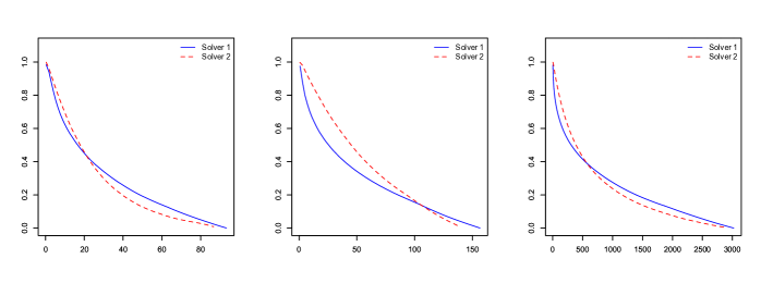
Figure 1: Relative errors plotted as function of computing time for Solver 1 and Solver 2.

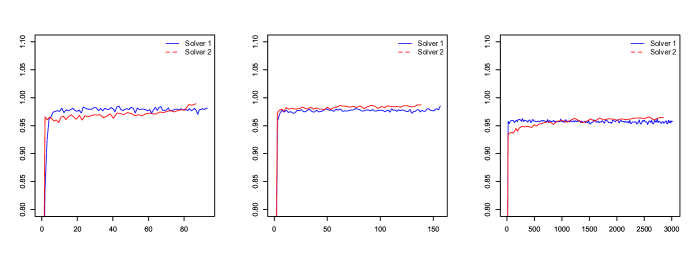
Figure 2: Statistic $\textsf{F}_{n}$ plotted as function of computing time for Solver 1 and Solver 2.

5 A non convex example: High-dimensional logistic regression with random effects

We numerically investigate the extension of our results to a situation where the assumptions H 2 and H 3 hold but H 1 is not in general satisfied and the domain $\Theta$ is not bounded. The numerical study below shows that the conclusions reached in section 2 and section 3 provide useful information to tune the design parameters of the algorithms.

5.1 The model

We model binary responses $\{Y_{i}\}_{i=1}^{N}\in\{0,1\}$ as $N$ conditionally independent realizations of a random effect logistic regression model,

$$Y_{i}|\mathbf{U}\stackrel{{\scriptstyle ind.}}{{\sim}}\textsf{Ber}\left(s(x_{i}^{\prime}\beta+\sigma z_{i}^{\prime}\mathbf{U})\right),\;\;1\leq i\leq N\;,$$ (17)

where $x_{i}\in\mathbb{R}^{p}$ is the vector of covariates, $z_{i}\in\mathbb{R}^{q}$ are (known) loading vector, $\textsf{Ber}(\alpha)$ denotes the Bernoulli distribution with parameter $\alpha\in\left[0,1\right]$, $s(x)=\mathrm{e}^{x}/(1+\mathrm{e}^{x})$ is the cumulative distribution function of the standard logistic distribution. The random effect $\mathbf{U}$ is assumed to be standard Gaussian $\mathbf{U}\sim\operatorname{N}_{q}(0,I)$.

The log-likelihood of the observations at $\theta=(\beta,\sigma)\in\mathbb{R}^{p}\times\left(0,\infty\right)$ is given by

$$\ell(\theta)=\log\int\prod_{i=1}^{N}s(x_{i}^{\prime}\beta+\sigma z_{i}^{\prime}\mathbf{u})^{Y_{i}}\left(1-s(x_{i}^{\prime}\beta+\sigma z_{i}^{\prime}\mathbf{u})\right)^{1-Y_{i}}\phi(\mathbf{u})\mathrm{d}\mathbf{u}\;,\\$$ (18)

where $\phi$ is the density of a $\mathbb{R}^{q}$-valued standard Gaussian random vector. The number of covariates $p$ is possibly larger than $N$, but only a very small number of these covariates are relevant which suggests to use the elastic-net penalty

$$\lambda\left(\frac{1-\alpha}{2}\|\beta\|_{2}^{2}+\alpha\|\beta\|_{1}\right)\;,$$ (19)

where $\lambda>0$ is the regularization parameter, $\|\beta\|_{r}=(\sum_{i=1}^{p}|\beta_{i}|^{r})^{1/r}$ and $\alpha\in\left[0,1\right]$ controls the trade-off between the $\ell^{1}$ and the $\ell^{2}$ penalties. In this example,

$$g(\theta)=\lambda\left(\frac{1-\alpha}{2}\|\beta\|_{2}^{2}+\alpha\|\beta\|_{1}\right)+\mathbbm{1}_{\left(0,+\infty\right)}(\sigma)\;,$$ (20)

where $\mathbbm{1}_{A}(x)=+\infty$ is $x\notin A$ and $0$ otherwise. Define the conditional log-likelihood of $\mathbf{Y}=(Y_{1},\dots,Y_{N})$ given $\mathbf{U}$ (the dependence upon $\mathbf{Y}$ is omitted) by

$$\ell_{c}(\theta|\mathbf{u})=\sum_{i=1}^{N}\left\{Y_{i}\left(x_{i}^{\prime}\beta+\sigma z_{i}^{\prime}\mathbf{u}\right)-\ln\left(1+\exp\left(x_{i}^{\prime}\beta+\sigma z_{i}^{\prime}\mathbf{u}\right)\right)\right\}\ \;,$$

and the conditional distribution of the random effect $\mathbf{U}$ given the observations $\mathbf{Y}$ and the parameter $\theta$

$$\pi_{\theta}(\mathbf{u})=\exp\left(\ell_{c}(\theta|\mathbf{u})-\ell(\theta)\right)\phi(\mathbf{u})\;.$$ (21)

The Fisher identity implies that the gradient of the log-likelihood (18) is given by

$$\nabla\ell(\theta) =\int\nabla_{\theta}\ell_{c}(\theta|\mathbf{u})\ \pi_{\theta}(\mathbf{u})\ \mathrm{d}\mathbf{u}=\int\left\{\sum_{i=1}^{N}(Y_{i}-s(x_{i}^{\prime}\beta+\sigma z_{i}^{\prime}\mathbf{u}))\begin{bmatrix}x_{i}\\ z_{i}^{\prime}\mathbf{u}\end{bmatrix}\right\}\pi_{\theta}(\mathbf{u})\ \mathrm{d}\mathbf{u}\;.$$

The Hessian of the log-likelihood $\ell$ is given by (see e.g.(McLachlan and Krishnan, 2008, Chapter 3))

$$\nabla^{2}\ell(\theta)=\mathbb{E}_{\pi_{\theta}}\left[\nabla^{2}_{\theta}\ell_{c}(\theta|\mathbf{U})\right]+\mathrm{Cov}_{\pi_{\theta}}\left(\nabla_{\theta}\ell_{c}(\theta|\mathbf{U})\right)$$

where $\mathbb{E}_{\pi_{\theta}}$ and $\mathrm{Cov}_{\pi_{\theta}}$ denotes the expectation and the covariance with respect to the distribution $\pi_{\theta}$, respectively. Since

$$\nabla_{\theta}^{2}\ell_{c}(\theta|\mathbf{u})=-\sum_{i=1}^{N}s(x_{i}^{\prime}\beta+\sigma z_{i}^{\prime}\mathbf{u})\,\left(1-s(x_{i}^{\prime}\beta+\sigma z_{i}^{\prime}\mathbf{u})\right)\begin{bmatrix}x_{i}\\ z_{i}^{\prime}\mathbf{u}\end{bmatrix}\begin{bmatrix}x_{i}\\ z_{i}^{\prime}\mathbf{u}\end{bmatrix}^{\prime}\;,$$

and $\sup_{\theta\in\Theta}\int\|\mathbf{u}\|^{2}\pi_{\theta}(\mathbf{u})\,\mathrm{d}\mathbf{u}<\infty$ (see section A), $\nabla^{2}\ell(\theta)$ is bounded on $\Theta$. Hence, $\nabla\ell(\theta)$ satisfies the Lipschitz condition showing that H 1 is satisfied.

5.2 Numerical application

The assumption H 3 is satisfied with $\pi_{\theta}$ given by (21) and

$$H_{\theta}(\mathbf{u})=-\sum_{i=1}^{N}(Y_{i}-F(x_{i}^{\prime}\beta+\sigma z_{i}^{\prime}\mathbf{u}))\begin{bmatrix}x_{i}\\ z_{i}^{\prime}\mathbf{u}\end{bmatrix}\;.$$ (22)

The distribution $\pi_{\theta}$ is sampled using the MCMC sampler proposed in Polson et al. (2013) based on data-augmentation. We write $-\nabla\ell(\theta)=\int_{\mathbb{R}^{q}\times\mathbb{R}^{N}}H_{\theta}(\mathbf{u})\tilde{\pi}_{\theta}(\mathbf{u},\mathbf{w})\ \mathrm{d}\mathbf{u}\mathrm{d}\mathbf{w}$ where $\tilde{\pi}_{\theta}(\mathbf{u},\mathbf{w})$ is defined for $\mathbf{u}\in\mathbb{R}^{q}$ and $\mathbf{w}=(w_{1},\cdots,w_{N})\in\mathbb{R}^{N}$ by

$$\tilde{\pi}_{\theta}(\mathbf{u},\mathbf{w})=\left(\prod_{i=1}^{N}\bar{\pi}_{\mathsf{PG}}\left(w_{i};x_{i}^{\prime}\beta+\sigma z_{i}^{\prime}\mathbf{u}\right)\right)\pi_{\theta}(\mathbf{u})\;;$$

in this expression, $\bar{\pi}_{\mathsf{PG}}(\cdot;c)$ is the density of the Polya-Gamma distribution on the positive real line with parameter $c$ given by

$$\bar{\pi}_{\mathsf{PG}}(w;c)=\cosh(c/2)\,\exp\left(-wc^{2}/2\right)\,\rho(w)\mathbbm{1}_{\mathbb{R}^{+}}(w)\;,$$

where $\rho(w)\propto\sum_{k\geq 0}(-1)^{k}(2k+1)\exp(-(2k+1)^{2}/(8w))w^{-3/2}$ (see (Biane et al., 2001, Section 3.1)). Thus, we have

$$\tilde{\pi}_{\theta}(\mathbf{u},\mathbf{w})=C_{\theta}\phi(\mathbf{u})\prod_{i=1}^{N}\exp\left(\sigma(Y_{i}-1/2)z_{i}^{\prime}\mathbf{u}-w_{i}(x_{i}^{\prime}\beta+\sigma z_{i}^{\prime}\mathbf{u})^{2}/2\right)\,\rho(w_{i})\mathbbm{1}_{\mathbb{R}^{+}}(w_{i})\;,$$

where $\ln C_{\theta}=-N\ln 2-\ell(\theta)+\sum_{i=1}^{N}(Y_{i}-1/2)x^{\prime}_{i}\beta$. This target distribution can be sampled using a Gibbs algorithm: given the current value $(\mathbf{u}^{t},\mathbf{w}^{t})$ of the chain, the next point is obtained by sampling $\mathbf{u}^{t+1}$ under the conditional distribution of $\mathbf{u}$ given $\mathbf{w}^{t}$, and $\mathbf{w}^{t+1}$ under the conditional distribution of $\mathbf{w}$ given $\mathbf{u}^{t+1}$. In the present case, these conditional distributions are given respectively by

$$\tilde{\pi}_{\theta}(\mathbf{u}|\mathbf{w})\equiv\operatorname{N}_{q}\left(\mu_{\theta}(\mathbf{w});\Gamma_{\theta}(\mathbf{w})\right)\qquad\tilde{\pi}_{\theta}(\mathbf{w}|\mathbf{u})=\prod_{i=1}^{N}\bar{\pi}_{\mathsf{PG}}(w_{i};|x_{i}^{\prime}\beta+\sigma z_{i}^{\prime}\mathbf{u}|)$$

with

$$\Gamma_{\theta}(\mathbf{w})=\left(I+\sigma^{2}\sum_{i=1}^{N}w_{i}z_{i}z_{i}^{\prime}\right)^{-1}\;,\qquad\mu_{\theta}(\mathbf{w})=\sigma\Gamma_{\theta}(\mathbf{w})\sum_{i=1}^{N}\left((Y_{i}-1/2)-w_{i}x_{i}^{\prime}\beta\right)z_{i}\;.$$ (23)

Exact samples of these conditional distributions can be obtained (see (Polson et al., 2013, Algorithm 1) for sampling under a Polya-Gamma distribution). It has been shown by Choi and Hobert (2013) that the Polya-Gamma Gibbs sampler is uniformly ergodic. Hence H 5 is satisfied with $W\equiv 1$. Checking H 6 is also straightforward.

We test the algorithms with $N=500$, $p=1,000$ and $q=5$. We generate the $N\times p$ covariates matrix $X$ columnwise, by sampling a stationary $\mathbb{R}^{N}$-valued autoregressive model with parameter $\rho=0.8$ and Gaussian noise $\sqrt{1-\rho^{2}}\,\mathcal{N}_{N}(0,I)$. We generate the vector of regressors $\beta_{\mathsf{true}}$ from the uniform distribution on $[1,5]$ and randomly set $98\%$ of the coefficients to zero. The variance of the random effect is set to $\sigma^{2}=0.1$. We consider a repeated measurement setting so that $z_{i}=e_{\lceil iq/N\rceil}$ where $\{e_{j},j\leq q\}$ is the canonical basis of $\mathbb{R}^{q}$ and $\lceil\cdot\rceil$ denotes the upper integer part. With such a simple expression for the random effect, we will be able to approximate the value $F(\theta)$ in order to illustrate the theoretical results obtained in this paper. We use the Lasso penalty ($\alpha=1$ in (19)) with $\lambda=30$.

We first illustrate the ability of Monte Carlo Proximal Gradient algorithms to find a minimizer of $F$. We compare the Monte Carlo proximal gradient algorithm

1. with fixed batch size: $\gamma_{n}=0.01/\sqrt{n}$ and $m_{n}=275$ (Algo 1); $\gamma_{n}=0.5/n$ and $m_{n}=275$ (Algo 2).

2. with increasing batch size: $\gamma_{n}=\gamma=0.005$, $m_{n}=200+n$ (Algo 3); $\gamma_{n}=\gamma=0.001$, $m_{n}=200+n$ (Algo 4); and $\gamma_{n}=0.05/\sqrt{n}$ and $m_{n}=270+\lceil\sqrt{n}\rceil$ (Algo 5).

Each algorithm is run for $150$ iterations. The batch sizes $\{m_{n},n\geq 0\}$ are chosen so that after $150$ iterations, each algorithm used approximately the same number of Monte Carlo samples. We denote by $\beta_{\infty}$ the value obtained at iteration $150$. A path of the relative error $\|\beta_{n}-\beta_{\infty}\|/\|\beta_{\infty}\|$ is displayed on Figure 3[right] for each algorithm; a path of the sensitivity $\mathsf{Sen}_{n}$ and of the precision $\mathsf{Prec}_{n}$ (see section 4 for the definition) are displayed on Figure 4. All these sequences are plotted versus the total number of Monte Carlo samples up to iteration $n$. These plots show that with a fixed batch-size (Algo 1 or Algo 2), the best convergence is obtained with a step size decreasing as $O(1/\sqrt{n})$; and for an increasing batch size (Algo 3 to Algo 5), it is better to choose a fixed step size. These findings are consistent with the results in section 3. On Figure 3[left], we report on the bottom row the indices $j$ such that $\beta_{\mathsf{true},j}$ is non null and on the rows above, the indices $j$ such that $\beta_{\infty,j}$ given by Algo 1 to Algo 5 is non null.

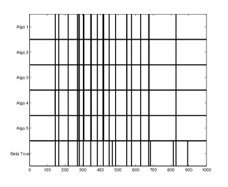
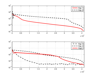
Figure 3: [left] The support of the sparse vector $\beta_{\infty}$ obtained by Algo 1 to Algo 5; for comparison, the support of $\beta_{\mathsf{true}}$ is on the bottom row. [right] Relative error along one path of each algorithm as a function of the total number of Monte Carlo samples.

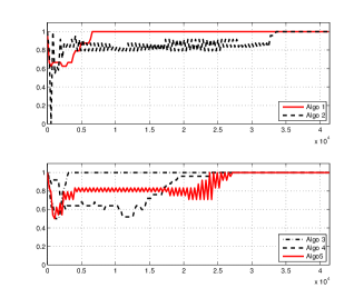
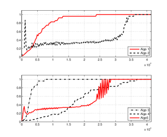
Figure 4: The sensitivity $\mathsf{Sen}_{n}$ [left] and the precision $\mathsf{Prec}_{n}$ [right] along a path, versus the total number of Monte Carlo samples up to time $n$

We now study the convergence of $\{F(\theta_{n}),n\in{\mathbb{N}}\}$ where $\theta_{n}$ is obtained by one of the algorithms described above. We repeat $50$ independent runs for each algorithm and estimate $\mathbb{E}\left[F(\theta_{n})\right]$ by the empirical mean over these runs. On Figure 5[left], $n\mapsto F(\theta_{n})$ is displayed for several runs of Algo 1 and Algo 3. The figure shows that all the paths have the same limiting value, which is approximately $F_{\star}=311$; we observed the same behavior on the $50$ runs of each algorithm. On Figure 5[right], we report the Monte Carlo estimation of $\mathbb{E}[F(\theta_{n})]$ versus the total number of Monte Carlo samples used up to iteration $n$ for the best strategies in the fixed batch size case (Algo 1) and in the increasing batch size case (Algo 3 and Algo 4).

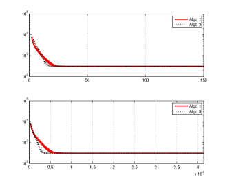
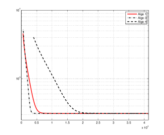
Figure 5: [left] $n\mapsto F(\theta_{n})$ for several independent runs. [right] $\mathbb{E}\left[F(\theta_{n})\right]$ versus the total number of Monte Carlo samples up to iteration $n$

6 Proofs

6.1 Preliminary lemmas

Lemma .

Assume that $g$ is lower semi-continuous and convex. For $\theta,\theta^{\prime}\in\Theta$ and $\gamma>0$

$$g\Big{(}\operatorname{Prox}_{\gamma,g}(\theta)\Big{)}-g(\theta^{\prime})\leq-\frac{1}{\gamma}\left\langle\operatorname{Prox}_{\gamma,g}(\theta)-\theta^{\prime},\operatorname{Prox}_{\gamma,g}(\theta)-\theta\right\rangle\;.$$ (24)

For any $\gamma>0$ and for any $\theta,\theta^{\prime}\in\Theta$,

$$\|\operatorname{Prox}_{\gamma,g}(\theta)-\operatorname{Prox}_{\gamma,g}(\theta^{\prime})\|^{2}+\|\big{(}\operatorname{Prox}_{\gamma,g}(\theta)-\theta\big{)}-\big{(}\operatorname{Prox}_{\gamma,g}(\theta^{\prime})-\theta^{\prime}\big{)}\|^{2}\leq\|\theta-\theta^{\prime}\|^{2}\;.$$ (25)

Proof.

See (Bauschke and Combettes, 2011, Propositions 4.2., 12.26 and  12.27).

Lemma .

Assume H 1 and let $\gamma\in\left(0,1/L\right]$. Then for all $\theta,\theta^{\prime}\in\Theta$,

$$-2\gamma\Big{(}F(\operatorname{Prox}_{\gamma,g}(\theta))-F(\theta^{\prime})\Big{)}\geq\|\operatorname{Prox}_{\gamma,g}(\theta)-\theta^{\prime}\|^{2}+2\left\langle\operatorname{Prox}_{\gamma,g}(\theta)-\theta^{\prime},\theta^{\prime}-\gamma\nabla f(\theta^{\prime})-\theta\right\rangle\;.$$ (26)

If in addition $f$ is convex, then for all $\theta,\theta^{\prime},\xi\in\Theta$,

$$-2\gamma\Big{(}F\big{(}\operatorname{Prox}_{\gamma,g}(\theta)\big{)}-F(\theta^{\prime})\Big{)}\geq\|\operatorname{Prox}_{\gamma,g}(\theta)-\theta^{\prime}\|^{2}\\ +2\left\langle\operatorname{Prox}_{\gamma,g}(\theta)-\theta^{\prime},\xi-\gamma\nabla f(\xi)-\theta\right\rangle-\|\theta^{\prime}-\xi\|^{2}\;.$$ (27)

Proof.

Since $\nabla f$ is Lipschitz, the descent lemma implies that for any $\gamma^{-1}\geq L$

$$f(p)-f(\theta^{\prime})\leq\left\langle\nabla f(\theta^{\prime}),p-\theta^{\prime}\right\rangle+\frac{1}{2\gamma}\|p-\theta^{\prime}\|^{2}\;.$$ (28)

This inequality applied with $p=\operatorname{Prox}_{\gamma,g}(\theta)$ combined with (24) yields (26). When $f$ is convex, $f(\xi)+\left\langle\nabla f(\xi),\theta^{\prime}-\xi\right\rangle-f(\theta^{\prime})\leq 0$ which, combined again with (24) and (28) applied with $(p,\theta^{\prime})\leftarrow(\operatorname{Prox}_{\gamma,g}(\theta),\xi)$ yields the result.

Lemma .

Assume H 1. Then for any $\gamma>0$, $\theta,\theta^{\prime}\in\Theta$,

$$\|\theta-\gamma\nabla f(\theta)-\theta^{\prime}+\gamma\nabla f(\theta^{\prime})\|\leq(1+\gamma L)\|\theta-\theta^{\prime}\|\;,$$ (29)

$$\|T_{\gamma}(\theta)-T_{\gamma}(\theta^{\prime})\|\leq(1+\gamma L)\|\theta-\theta^{\prime}\|\;.$$ (30)

If in addition $f$ is convex then for any $\gamma\in\left(0,2/L\right]$,

$$\|\theta-\gamma\nabla f(\theta)-\theta^{\prime}+\gamma\nabla f(\theta^{\prime})\|\leq\|\theta-\theta^{\prime}\|\;,$$ (31)

$$\|T_{\gamma}(\theta)-T_{\gamma}(\theta^{\prime})\|\leq\|\theta-\theta^{\prime}\|\;.$$ (32)

Proof.

(30) and (32) follows from (29) and (31) respectively by the Lipschitz property of the proximal map $\operatorname{Prox}_{\gamma,g}$ (see Section 6.1). (29) follows directly from the Lipschitz property of $f$. It remains to prove (31). Since $f$ is a convex function with Lipschitz-continuous gradients, (Nesterov, 2004, Theorem 2.1.5) shows that, for all $\theta,\theta^{\prime}\in\Theta$, $L\,\left\langle\nabla f(\theta)-\nabla f(\theta^{\prime}),\theta-\theta^{\prime}\right\rangle\geq\|\nabla f(\theta)-\nabla f(\theta^{\prime})\|^{2}$. The result follows.

Lemma .

Assume H 1. Set $S_{\gamma}(\theta)\stackrel{{\scriptstyle\mathrm{def}}}{{=}}\operatorname{Prox}_{\gamma,g}(\theta-\gamma H)$ and $\eta\stackrel{{\scriptstyle\mathrm{def}}}{{=}}H-\nabla f(\theta)$. For any $\theta\in\Theta$ and $\gamma>0$,

$$\|T_{\gamma}(\theta)-S_{\gamma}(\theta)\|\leq\gamma\|\eta\|\;.$$ (33)

Proof.

We have $\|T_{\gamma}(\theta)-S_{\gamma}(\theta)\|=\|\operatorname{Prox}_{\gamma,g}(\theta-\gamma\nabla f(\theta))-\operatorname{Prox}_{\gamma,g}(\theta-\gamma H)\|$ and (33) follows from Section 6.1.

6.2 Proof of section 2

6.2.1 Proof of section 2

Set $w_{n}=v_{n}+\sum_{k\geq n+1}\xi_{k}+M$ with $M\stackrel{{\scriptstyle\mathrm{def}}}{{=}}-\inf_{n}\sum_{k\geq n}\xi_{k}$ so that $\inf_{n}w_{n}\geq 0$. Then

$$0\leq w_{n+1}\leq v_{n}-\chi_{n+1}+\xi_{n+1}+\sum_{k\geq n+2}\xi_{k}+M\leq w_{n}-\chi_{n+1}\;.$$

$\{w_{n},\;n\in{\mathbb{N}}\}$ is non-negative and non increasing; therefore it converges. Furthermore, $0\leq\sum_{k=0}^{n}\chi_{k}\leq w_{0}$ so that $\sum_{n}\chi_{n}<\infty$. The convergence of $\{w_{n},\;n\in{\mathbb{N}}\}$ also implies the convergence of $\{v_{n},\;n\in{\mathbb{N}}\}$. This concludes the proof.

6.2.2 Proof of Theorem 1

Let $\theta_{\star}\in\mathcal{L}$, which is not empty by H 2; note that $F(\theta_{\star})=\min F$. We have by (27) applied with $\theta\leftarrow\theta_{n}-\gamma_{n+1}H_{n+1}$, $\xi\leftarrow\theta_{n}$, $\theta^{\prime}\leftarrow\theta_{\star}$, $\gamma\leftarrow\gamma_{n+1}$

$$\|\theta_{n+1}-\theta_{\star}\|^{2} \leq\|\theta_{n}-\theta_{\star}\|^{2}-2\gamma_{n+1}\left(F(\theta_{n+1})-\min F\right)-2\gamma_{n+1}\left\langle\theta_{n+1}-\theta_{\star},\eta_{n+1}\right\rangle\;.$$

We write $\theta_{n+1}-\theta_{\star}=\theta_{n+1}-T_{\gamma_{n+1}}(\theta_{n})+T_{\gamma_{n+1}}(\theta_{n})-\theta_{\star}.$ By Section 6.1, $\|\theta_{n+1}-T_{\gamma_{n+1}}(\theta_{n})\|\leq\gamma_{n+1}\|\eta_{n+1}\|$ so that,

$$-\left\langle\theta_{n+1}-\theta_{\star},\eta_{n+1}\right\rangle\leq\gamma_{n+1}\|\eta_{n+1}\|^{2}-\left\langle T_{\gamma_{n+1}}(\theta_{n})-\theta_{\star},\eta_{n+1}\right\rangle\;.$$

Hence,

$$\|\theta_{n+1}-\theta_{\star}\|^{2}\leq\|\theta_{n}-\theta_{\star}\|^{2}-2\gamma_{n+1}\left(F(\theta_{n+1})-\min F\right)\\ +2\gamma_{n+1}^{2}\|\eta_{n+1}\|^{2}-2\gamma_{n+1}\left\langle T_{\gamma_{n+1}}(\theta_{n})-\theta_{\star},\eta_{n+1}\right\rangle\;.$$ (34)

Under (7) and (34), section 2 shows that $\sum_{n}\gamma_{n}\left(F(\theta_{n})-\min F\right)<\infty$ and $\lim_{n}\|\theta_{n}-\theta_{\star}\|$ exists. This implies that $\sup_{n}\|\theta_{n}\|<\infty$. Since $\sum_{n}\gamma_{n}=+\infty$, there exists a subsequence $\{\theta_{\phi_{n}},n\in{\mathbb{N}}\}$ such that $\lim_{n}F(\theta_{\phi_{n}})=\min F$. The sequence $\{\theta_{\phi_{n}},n\geq 0\}$ being bounded, we can assume without loss of generality that there exists $\theta_{\infty}\in\mathbb{R}^{d}$ such that $\lim_{n}\theta_{\phi_{n}}=\theta_{\infty}$.

Let us prove that $\theta_{\infty}\in\mathcal{L}$. Since $g$ is lower semi-continuous on $\Theta$, $\liminf_{n}g(\theta_{\phi_{n}})\geq g(\theta_{\infty})$ so that $\theta_{\infty}\in\Theta$. Since $F$ is lower semi-continuous on $\Theta$, we have

$$\min F=\liminf_{n\to\infty}F(\theta_{\phi_{n}})\geq F(\theta_{\infty})\geq\min F\;,$$

showing that $F(\theta_{\infty})=\min F$.

By (34), for any $m$ and $n\geq\phi_{m}$

$$\|\theta_{n+1}-\theta_{\infty}\|^{2}\leq\|\theta_{\phi_{m}}-\theta_{\infty}\|^{2}-2\sum_{k=\phi_{m}}^{n}\gamma_{k+1}\{\left\langle T_{\gamma_{k+1}}(\theta_{k})-\theta_{\infty},\eta_{k+1}\right\rangle+\gamma_{k+1}\|\eta_{k+1}\|^{2}\}\;.$$

For any $\epsilon>0$, there exists $m$ such that the RHS is upper bounded by $\epsilon$. Hence, for any $n\geq\phi_{m}$, $\|\theta_{n+1}-\theta_{\infty}\|^{2}\leq\epsilon$, which proves the convergence of $\{\theta_{n},\;n\in{\mathbb{N}}\}$ to $\theta_{\infty}$.

6.2.3 Proof of Theorem 2

Let $\theta_{\star}\in\mathcal{L}$; note that $F(\theta_{\star})=\min F$. We first apply (27) with $\theta\leftarrow\theta_{j}-\gamma_{j+1}H_{j+1}$, $\xi\leftarrow\theta_{j}$, $\theta^{\prime}\leftarrow\theta_{\star}$, $\gamma\leftarrow\gamma_{j+1}$:

$$F(\theta_{j+1})-\min F \leq(2\gamma_{j+1})^{-1}\,\left(\|\theta_{j}-\theta_{\star}\|^{2}-\|\theta_{j+1}-\theta_{\star}\|^{2}\right)-\left\langle\theta_{j+1}-\theta_{\star},\eta_{j+1}\right\rangle\;.$$

Multiplying both sides by $a_{j+1}$ gives:

$$a_{j+1}\Big{(}F(\theta_{j+1})-\min F\Big{)}\leq\frac{1}{2}\left(\frac{a_{j+1}}{\gamma_{j+1}}-\frac{a_{j}}{\gamma_{j}}\right)\|\theta_{j}-\theta_{\star}\|^{2}+\frac{a_{j}}{2\gamma_{j}}\|\theta_{j}-\theta_{\star}\|^{2}\\ -\frac{a_{j+1}}{2\gamma_{j+1}}\|\theta_{j+1}-\theta_{\star}\|^{2}-a_{j+1}\left\langle\theta_{j+1}-\theta_{\star},\eta_{j+1}\right\rangle.$$

Summing from $j=0$ to $n-1$ gives

$$\frac{a_{n}}{2\gamma_{n}}\|\theta_{n}-\theta_{\star}\|^{2}+\sum_{j=1}^{n}a_{j}\{F(\theta_{j})-\min F\}\leq\frac{1}{2}\sum_{j=1}^{n}\left(\frac{a_{j}}{\gamma_{j}}-\frac{a_{j-1}}{\gamma_{j-1}}\right)\|\theta_{j-1}-\theta_{\star}\|^{2}\\ -\sum_{j=1}^{n}a_{j}\left\langle\theta_{j}-\theta_{\star},\eta_{j}\right\rangle+\frac{a_{0}}{2\gamma_{0}}\|\theta_{0}-\theta_{\star}\|^{2}\;.$$ (35)

We decompose $\left\langle\theta_{j}-\theta_{\star},\eta_{j}\right\rangle$ as follows:

$$\left\langle\theta_{j}-\theta_{\star},\eta_{j}\right\rangle=\left\langle\theta_{j}-T_{\gamma_{j}}(\theta_{j-1}),\eta_{j}\right\rangle+\left\langle T_{\gamma_{j}}(\theta_{j-1})-\theta_{\star},\eta_{j}\right\rangle\;.$$

By Section 6.1, we get $\left|\left\langle\theta_{j}-T_{\gamma_{j}}(\theta_{j-1}),\eta_{j}\right\rangle\right|\leq\gamma_{j}\|\eta_{j}\|^{2}$ which concludes the proof.

6.3 Proof of Section 3.1

The proof of Theorem 3 is given in the case $m=1$; we simply denote by $X_{n}$ the sample $X_{n}^{(1)}$. The proof for the case $m>1$ can be adapted from the proof below, by substituting the functions $H_{\theta}(x)$ and $W(x)$ by

$$\overline{H}_{\theta}(x_{1},\cdots,x_{m})=\frac{1}{m}\sum_{k=1}^{m}H_{\theta}(x_{k})\qquad\overline{W}(x_{1},\cdots,x_{m})=\frac{1}{m}\sum_{k=1}^{m}W(x_{k})\;;$$

the kernel $P_{\theta}$ and its invariant measure $\pi_{\theta}$ by

$$\overline{P}_{\theta}(x_{1},\cdots,x_{m};B) =\idotsint P_{\theta}(x_{m},\mathrm{d}y_{1})\,\prod_{k=2}^{m}P_{\theta}(y_{k-1},\mathrm{d}y_{k})\mathbbm{1}_{B}(y_{1},\dots,y_{m})\;,$$

$$\overline{\pi}_{\theta}(B) =\idotsint\pi_{\theta}(\mathrm{d}y_{1})\,\prod_{k=2}^{m}P_{\theta}(y_{k-1},\mathrm{d}y_{k})\mathbbm{1}_{B}(y_{1},\dots,y_{m})\;,$$

for any $(x_{1},\dots,x_{m})\in\mathsf{X}^{n}$ and $B\in\mathcal{X}^{\times n}$.

6.3.1 Preliminary results

Proposition .

Assume that $g$ is proper convex and Lipschitz on $\Theta$ with Lipschitz constant $K$. Then, for all $\theta\in\Theta$,

$$\left\|\operatorname{Prox}_{\gamma,g}(\theta)-\theta\right\|\leq K\gamma\;.$$ (36)

Proof.

For all $\theta\in\Theta$, we get by Section 6.1

$$0\leq\gamma^{-1}\left\|\theta-\operatorname{Prox}_{\gamma,g}(\theta)\right\|^{2}\leq g(\theta)-g(\operatorname{Prox}_{\gamma,g}(\theta))\leq K\left\|\theta-\operatorname{Prox}_{\gamma,g}(\theta)\right\|\;.$$

Proposition .

Assume H 1, H 2 and $\Theta$ is bounded. Then

$$\sup_{\gamma\in\left(0,1/L\right]}\sup_{\theta\in\Theta}\left\|T_{\gamma}(\theta)\right\|<\infty\;.$$

If in addition H 6-(ii) holds, then there exists a constant $C$ such that for any $\theta,\bar{\theta}\in\Theta$, $\gamma,\bar{\gamma}\in\left(0,1/L\right]$

$$\left\|T_{\gamma}(\theta)-T_{\bar{\gamma}}(\bar{\theta})\right\|\leq C\left(\gamma+\bar{\gamma}+\|\theta-\bar{\theta}\|\right)\;.$$

Proof.

Let $\theta_{\star}$ such that for any $\gamma>0$, $\theta_{\star}=T_{\gamma}(\theta_{\star})$ (such a point exists by H 2 and (4)). We write $T_{\gamma}(\theta)=\left(T_{\gamma}(\theta)-\theta_{\star}\right)+\theta_{\star}$. By Section 6.1, there exists a constant $C$ such that for any $\theta\in\Theta$ and any $\gamma\in\left(0,1/L\right]$, $\left\|T_{\gamma}(\theta)-\theta_{\star}\right\|\leq 2\,\left\|\theta-\theta_{\star}\right\|\leq{\color[rgb]{0,0,0}2}\left\|\theta\right\|+{\color[rgb]{0,0,0}2}\left\|\theta_{\star}\right\|$. This concludes the proof of the first statement. We write $T_{\gamma}(\theta)-T_{\bar{\gamma}}(\bar{\theta})=T_{\gamma}(\theta)-T_{\bar{\gamma}}(\theta)+T_{\bar{\gamma}}(\theta)-T_{\bar{\gamma}}(\bar{\theta})$. By Section 6.1

$$\left\|T_{\bar{\gamma}}(\theta)-T_{\bar{\gamma}}(\bar{\theta})\right\|\leq\left\|\theta-\bar{\theta}-\bar{\gamma}\nabla f(\theta)+\bar{\gamma}\nabla f(\bar{\theta})\right\|\leq\|\theta-\bar{\theta}\|+\bar{\gamma}\sup_{\theta\in\Theta}\|\nabla f(\theta)\|\;.$$

By H 1 and since $\Theta$ is bounded, $\sup_{\theta\in\Theta}\|\nabla f(\theta)\|<\infty$. In addition, using again Section 6.1,

$$\left\|T_{\gamma}(\theta)-T_{\bar{\gamma}}(\theta)\right\| \leq\left(\gamma+\bar{\gamma}\right)\ \sup_{\theta\in\Theta}\|\nabla f(\theta)\|+\left\|\operatorname{Prox}_{\gamma,g}(\theta)-\operatorname{Prox}_{\bar{\gamma},g}(\theta)\right\|\;.$$

We conclude by using

$$\left\|\operatorname{Prox}_{\bar{\gamma},g}(\theta)-\operatorname{Prox}_{\gamma,g}(\theta)\right\| \leq\left\|\operatorname{Prox}_{\bar{\gamma},g}(\theta)-\theta\right\|+\left\|\theta-\operatorname{Prox}_{\gamma,g}(\theta)\right\|$$

$$\leq\left(\gamma+\bar{\gamma}\right)\ \sup_{\gamma\in\left(0,1/L\right]}\sup_{\theta\in\Theta}\gamma^{-1}\,\left\|\operatorname{Prox}_{\gamma,g}(\theta)-\theta\right\|\;.$$

Lemma .

Assume H 5 and H 6-(i).

1. There exists a measurable function $(\theta,x)\mapsto\widehat{H}_{\theta}(x)$ such that $\sup_{\theta\in\Theta}\left|\widehat{H}_{\theta}\right|_{W}<\infty$ and for any $(\theta,x)\in\Theta\times\mathsf{X}$,

   $$\widehat{H}_{\theta}(x)-P_{\theta}\widehat{H}_{\theta}(x)=H_{\theta}(x)-\int H_{\theta}(y)\pi_{\theta}(\mathrm{d}y)\;.$$ (37)

2. There exists a constant $C$ such that for any $\theta,\theta^{\prime}\in\Theta$,

   $$\left\|P_{\theta}\widehat{H}_{\theta}-P_{\theta^{\prime}}\widehat{H}_{\theta^{\prime}}\right\|_{W}\leq C\ \left\|\theta-\theta^{\prime}\right\|\;.$$

Proof.

See (Fort et al., 2011, Lemma 4.2).

Lemma .

Assume H 4 and H 5. Then, $\sup_{n}\mathbb{E}\left[W^{p}(X_{n})\right]<\infty$.

Proof.

Conditionnally to the past $\mathcal{F}_{j-1}$, the conditional distribution of $X_{j}$ is $P_{\theta_{j-1}}(X_{j-1},\cdot)$. Therefore, we write

$$\mathbb{E}\left[W^{p}(X_{n})\right]=\mathbb{E}\left[{\mathbb{E}}\left[\left.W^{p}(X_{n})\,\right|\mathcal{F}_{n-1}\right]\right]=\mathbb{E}\left[P_{\theta_{n-1}}W^{p}(X_{n-1})\right].$$

We then use the drift inequality to obtain $\mathbb{E}\left[W^{p}(X_{n})\right]\leq\lambda\mathbb{E}\left[W^{p}(X_{n-1})\right]+b$. The proof then follows from a trivial induction.

Lemma .

Assume H 1, H 6-(ii) and $\Theta$ is bounded. There exists a constant $C$ such that w.p.1, for all $n\geq 0$,

$$\left\|\theta_{n+1}-\theta_{n}\right\|\leq C\gamma_{n+1}\left(1+\left\|\eta_{n+1}\right\|\right)\;.$$

Proof.

We write

$$\theta_{n+1}-\theta_{n}=\theta_{n+1}-\operatorname{Prox}_{\gamma_{n+1},g}(\theta_{n})+\operatorname{Prox}_{\gamma_{n+1},g}(\theta_{n})-\theta_{n}.$$

Since by Section 6.1, $\theta\mapsto\operatorname{Prox}_{\gamma,g}(\theta)$ is Lipschitz for any $\gamma>0$, we get

$$\left\|\theta_{n+1}-\operatorname{Prox}_{\gamma_{n+1},g}(\theta_{n})\right\|=\left\|\operatorname{Prox}_{\gamma_{n+1},g}(\theta_{n}-\gamma_{n+1}\eta_{n+1}-\gamma_{n+1}\nabla f(\theta_{n}))-\operatorname{Prox}_{\gamma_{n+1},g}\left(\theta_{n}\right)\right\|$$

$$\quad\leq\gamma_{n+1}\left\|\eta_{n+1}+\nabla f(\theta_{n})\right\|\leq\gamma_{n+1}\left(\left\|\eta_{n+1}\right\|+\sup_{\theta\in\Theta}\left\|\nabla f(\theta)\right\|\right)\;.$$

By H 1, w.p.1. $\sup_{\theta\in\Theta}\left\|\nabla f(\theta)\right\|<\infty$; hence, there exists $C_{1}$ such that w.p.1. for all $n\geq 0$, $\left\|\theta_{n+1}-\operatorname{Prox}_{\gamma_{n+1},g}(\theta_{n})\right\|\leq C_{1}\gamma_{n+1}\left(1+\left\|\eta_{n+1}\right\|\right)$. Finally, under H 6-(ii), there exists a constant $C_{2}$ such that, w.p.1.,

$$\sup_{n}\gamma_{n+1}^{-1}\left\|\operatorname{Prox}_{\gamma_{n+1},g}(\theta_{n})-\theta_{n}\right\|\leq\sup_{\gamma\in\left(0,1/L\right]}\sup_{\theta\in\Theta}\gamma^{-1}\left\|\operatorname{Prox}_{\gamma,g}(\theta)-\theta\right\|\leq C_{2}\;.$$

This concludes the proof.

Lemma .

Assume H 1, H 4, H 5 and $\Theta$ is bounded. There exists a constant $C$ such that w.p.1, for all $n\geq 0$, $\left\|\eta_{n+1}\right\|\leq CW(X_{n+1})$.

Proof.

By H 4 and H 5, $\left\|\eta_{n+1}\right\|\leq\left(\sup_{\theta\in\Theta}\left|H_{\theta}\right|_{W}\right)\,W(X_{n+1})+\sup_{\theta\in\Theta}\|\nabla f(\theta)\|$. The result follows since $\nabla f$ is Lipschitz by H 1, and since $W\geq 1$.

6.3.2 Proof of Theorem 3

The proof of the almost-sure convergence consists in verifying the assumptions of Theorem 1. Let us start with the proof that almost-surely, $\sum_{n}\gamma_{n+1}^{2}\|\eta_{n+1}\|^{2}<\infty$. This property is a consequence of Section 6.3.2 applied with $a_{n}\leftarrow\gamma_{n}^{2}$. It remains to prove that almost-surely

$$\sum_{n}\gamma_{n}\eta_{n}<\infty,\qquad\sum_{n}\gamma_{n+1}\left\langle T_{\gamma_{n+1}}(\theta_{n}),\eta_{n+1}\right\rangle<\infty;$$

note that they are both of the form $\sum_{n}\gamma_{n+1}\mathsf{A}_{\gamma_{n+1}}(\theta_{n})\eta_{n+1}$ with, respectively, $\mathsf{A}_{\gamma}(\theta)$ equal to the identity matrix, and $\mathsf{A}_{\gamma}(\theta)=T_{\gamma}(\theta)$. In the case the Monte Carlo is unbiased, we apply Section 6.3.2 with $a_{n}\leftarrow\gamma_{n}$ and $A_{\gamma}(\theta)$ equal to the identity matrix and we obtain the almost-sure convergence of $\sum_{n}\gamma_{n}\eta_{n}$; we then apply Section 6.3.2 with $a_{n}\leftarrow\gamma_{n}$ and $A_{\gamma}(\theta)=T_{\gamma}(\theta)$, and we obtain the almost-sure convergence of $\sum_{n}\gamma_{n+1}\left\langle T_{\gamma_{n+1}}(\theta_{n}),\eta_{n+1}\right\rangle$ - note that by Section 6.3.1, $T_{\gamma}(\theta)$ satisfies the assumptions on $\mathsf{A}_{\gamma}(\theta)$. In the case the Monte Carlo is biased, the steps are the same except we use Section 6.3.2 instead of Section 6.3.2.

For the control of the moments, we use Theorem 2 and again Section 6.3.2 and Section 6.3.2 for the unbiased case (or Section 6.3.2 for the biased case).

Lemma .

Assume H 1, H 4, H 5 and $\Theta$ is bounded.

1. If $a_{k}\geq 0$ and $\sum_{k=1}^{\infty}a_{k}<\infty$ then with probability one, $\sum_{n\geq 1}a_{n}\|\eta_{n}\|^{2}<\infty$.

2. for any $q\in\left[1,p/2\right]$, there exists a constant $C$ such that for any non-negative numbers $\{a_{1},\cdots,a_{n}\}$,

   $$\left\|\sum_{k=1}^{n}a_{k}\|\eta_{k}\|^{2}\right\|_{L^{q}}\leq C\,\sum_{k=1}^{n}a_{k}\;.$$

Proof.

We write

$$\mathbb{E}\left[\sum_{n\geq 0}a_{n+1}\|\eta_{n+1}\|^{2}\right]\leq\sup_{n}\left(\mathbb{E}\left[\|\eta_{n+1}\|^{2}\right]\right)\,\sum_{n\geq 0}a_{n+1}\;.$$

By Section 6.3.1 and Section 6.3.1, $\sup_{n}\left\|\eta_{n+1}\right\|_{L^{2}}<\infty$ so the RHS is finite. By the Minkovski inequality, we write since $a_{k}>0$,

$$\left\|\sum_{k=0}^{n}a_{k+1}\|\eta_{k+1}\|^{2}\right\|_{L^{q}}\leq\sup_{n}\left\|\eta_{n}\right\|_{L^{2q}}^{2}\,\sum_{k=1}^{n+1}a_{k}\;.$$

The supremum is finite by Section 6.3.1 and Section 6.3.1.

Proposition .

Assume H 1, H 3, H 4, H 5, $\Theta$ is bounded and the Monte Carlo approximation is unbiased. Let $\{a_{n},\;n\in{\mathbb{N}}\}$ be a deterministic positive sequence and $\{\mathsf{A}_{\gamma}(\theta),\gamma\in\left(0,1/L\right],\theta\in\Theta\}$ be deterministic matrices such that

$$\sup_{\gamma\in\left(0,1/L\right]}\sup_{\theta\in\Theta}\|\mathsf{A}_{\gamma}(\theta)\|<\infty\;.$$ (38)

1. If $\sum_{n\geq 0}a_{n}^{2}<\infty$, then the series $\sum_{n\geq 0}a_{n+1}\mathsf{A}_{\gamma_{n+1}}(\theta_{n})\eta_{n+1}$ converges $\mathbb{P}$-a.s.

2. For any $q\in\left(1,p/2\right]$, there exists a constant $C$ such that

   $$\left\|\sum_{k=0}^{n}a_{k+1}\mathsf{A}_{\gamma_{k+1}}(\theta_{k})\eta_{k+1}\right\|_{L^{q}}\leq C\ \left(\sum_{k=0}^{n}a_{k+1}^{2}\right)^{1/2}\;.$$

Proof.

Since $\theta_{n}\in\mathcal{F}_{n}$, we have $\mathbb{E}\left[a_{n+1}\mathsf{A}_{\gamma_{n+1}}(\theta_{n})\ \eta_{n+1}|\mathcal{F}_{n}\right]=0$, thus showing that $\{M_{n}=\sum_{k=0}^{n}a_{k+1}\mathsf{A}_{\gamma_{k+1}}(\theta_{k})\eta_{k+1},n\in{\mathbb{N}}\}$ is a martingale. This martingale converges almost-surely if $S=\sum_{n\geq 0}a_{n+1}^{2}\|\mathsf{A}_{\gamma_{n+1}}(\theta_{n})\|^{2}\|\eta_{n+1}\|^{2}<\infty$ $\mathbb{P}$-a.s. (see e.g. (Hall and Heyde, 1980, Theorem 2.17)). Using (38) and Section 6.3.2, $S<\infty$ $\mathbb{P}$-a.s.

Consider now the $L^{q}$-moment of $M_{n}$. We apply (Hall and Heyde, 1980, Theorem 2.10): for any $q\in\left(1,p/2\right]$, there exists a constant $C$ such that for any $n\geq 0$,

$$\left\|\sum_{k=0}^{n}a_{k+1}\mathsf{A}_{\gamma_{k+1}}(\theta_{k})\eta_{k+1}\right\|_{L^{q}}\leq C\left(\sum_{k=0}^{n}\left\|a_{k+1}\mathsf{A}_{\gamma_{k+1}}(\theta_{k})\eta_{k+1}\right\|_{L^{q}}^{2}\right)^{1/2}\;.$$

Section 6.3.1 and Section 6.3.1 imply that $\sup_{n}\left\|\eta_{n+1}\right\|_{L^{q}}<\infty$; we then conclude with (38).

Proposition .

Assume H 1, H 3–H 6 and $\Theta$ is bounded. Let $\{a_{n},n\geq 0\}$ be a positive sequence and $\{\mathsf{A}_{\gamma}(\theta),\gamma\in\left(0,1/L\right],\theta\in\Theta\}$ be (deterministic) function-valued matrices such that there exists $C_{\mathsf{A}}$ and for any $\gamma,\bar{\gamma}\in\left(0,1/L\right]$ and $\theta,\bar{\theta}\in\Theta$

$$\sup_{\gamma\in\left(0,1/L\right]}\sup_{\theta\in\Theta}\|\mathsf{A}_{\gamma}(\theta)\|<\infty\;,\qquad\left\|\mathsf{A}_{\gamma}(\theta)-\mathsf{A}_{\bar{\gamma}}(\bar{\theta})\right\|\leq C_{\mathsf{A}}\left(\gamma+\bar{\gamma}+\left\|\theta-\bar{\theta}\right\|\right)\;.$$ (39)

1. If $\sum_{n}a_{n}\gamma_{n}<\infty$, $\sum_{n}a_{n}^{2}<\infty$ and $\sum_{n}|a_{n+1}-a_{n}|<\infty$ then the series $\sum_{n\geq 0}a_{n+1}\mathsf{A}_{\gamma_{n+1}}(\theta_{n})\eta_{n+1}$ converges $\mathbb{P}$-a.s.

2. For any $q\in\left(1,p/2\right]$, there exists a constant $C$ such that

   $$\left\|\sum_{k=0}^{n}a_{k+1}\mathsf{A}_{\gamma_{k+1}}(\theta_{k})\eta_{k+1}\right\|_{L^{q}}\leq C\ \left\{1+\left(\sum_{k=0}^{n}a_{k+1}^{2}\right)^{1/2}+\sum_{k=1}^{n}\left|a_{k+1}-a_{k}\right|+\sum_{k=1}^{n}a_{k}\gamma_{k}\right\}\;.$$

Proof.

1. By H 4 and Section 6.3.1-(i), we write

   $$\eta_{n+1} =\widehat{H}_{\theta_{n}}(X_{n+1})-P_{\theta_{n}}\widehat{H}_{\theta_{n}}(X_{n+1})$$

   $$=\left(\widehat{H}_{\theta_{n}}(X_{n+1})-P_{\theta_{n}}\widehat{H}_{\theta_{n}}(X_{n})\right)+\left(P_{\theta_{n}}\widehat{H}_{\theta_{n}}(X_{n})-P_{\theta_{n+1}}\widehat{H}_{\theta_{n+1}}(X_{n+1})\right)$$

   $$+\left(P_{\theta_{n+1}}\widehat{H}_{\theta_{n+1}}(X_{n+1})-P_{\theta_{n}}\widehat{H}_{\theta_{n}}(X_{n+1})\right)\;.$$

   We prove successively that w.p.1,

   $$\sum_{n}a_{n+1}\mathsf{A}_{\gamma_{n+1}}(\theta_{n})\ \left(\widehat{H}_{\theta_{n}}(X_{n+1})-P_{\theta_{n}}\widehat{H}_{\theta_{n}}(X_{n})\right)<\infty\;,$$ (40)

   $$\sum_{n\geq 0}a_{n+1}\mathsf{A}_{\gamma_{n+1}}(\theta_{n})\ \left(P_{\theta_{n}}\widehat{H}_{\theta_{n}}(X_{n})-P_{\theta_{n+1}}\widehat{H}_{\theta_{n+1}}(X_{n+1})\right)<\infty\;,$$ (41)

   $$\sum_{n\geq 0}a_{n+1}\mathsf{A}_{\gamma_{n+1}}(\theta_{n})\left(P_{\theta_{n+1}}\widehat{H}_{\theta_{n+1}}(X_{n+1})-P_{\theta_{n}}\widehat{H}_{\theta_{n}}(X_{n+1})\right)<\infty\;.$$ (42)

   Proof of (40) By H 4, $\{\widehat{H}_{\theta_{n}}(X_{n+1})-P_{\theta_{n}}\widehat{H}_{\theta_{n}}(X_{n}),n\in{\mathbb{N}}\}$ is a martingale increment w.r.t. the filtration $\{\mathcal{F}_{n},n\geq 0\}$. The proof is along the same lines as the proof of Section 6.3.2 upon noting that by Section 6.3.1 and H 5, there exists $C$ such that w.p.1 for all $n\geq 0$,

   $$\|\widehat{H}_{\theta_{n}}(X_{n+1})-P_{\theta_{n}}\widehat{H}_{\theta_{n}}(X_{n})\|\leq C\,\left(W(X_{n+1})+W(X_{n})\right)\;.$$

   Proof of (41) The sum is equal to $\sum_{n\geq 0}\Delta_{n+1}P_{\theta_{n}}\widehat{H}_{\theta_{n}}(X_{n})$ with $\Delta_{n+1}=a_{n+1}\mathsf{A}_{\gamma_{n+1}}(\theta_{n})-a_{n}\mathsf{A}_{\gamma_{n}}(\theta_{n-1})$. On one hand, by Section 6.3.1 and H 5, there exists $C$ such that w.p.1 for all $n\geq 0$,

   $$\left\|P_{\theta_{n}}\widehat{H}_{\theta_{n}}(X_{n})\right\|\leq C\,W(X_{n})\;.$$

   On the other hand, by (39), Section 6.3.1 and Section 6.3.1, there exists $C$ such that a.s.

   $$\text{for all $n\geq 0$},\qquad\left\|\Delta_{n+1}\right\|\leq C\Big{(}\left|a_{n+1}-a_{n}\right|+a_{n}\left(\gamma_{n}+\gamma_{n+1}\right)\Big{)}W(X_{n})\;.$$

   By Section 6.3.1, $\sup_{n}\mathbb{E}\left[W^{2}(X_{n})\right]<\infty$. Therefore, by (39) and the assumptions on $\{a_{n},n\geq 0\}$, we have $\sum_{n}\mathbb{E}\left[\left\|\Delta_{n+1}\ P_{\theta_{n}}\widehat{H}_{\theta_{n}}(X_{n})\right\|\right]<\infty$; which concludes the proof.

   Proof of (42) By (39) and Section 6.3.1, there exists a constant $C$ such that w.p.1 for any $n$

   $$\left\|\mathsf{A}_{\gamma_{n+1}}(\theta_{n})\left(P_{\theta_{n+1}}\widehat{H}_{\theta_{n+1}}(X_{n+1})-P_{\theta_{n}}\widehat{H}_{\theta_{n}}(X_{n+1})\right)\right\|\leq C\,\left\|\theta_{n+1}-\theta_{n}\right\|\,W(X_{n+1})\;.$$

   By Section 6.3.1 and Section 6.3.1, there exists a constant $C$ such that w.p.1,

   $$\text{for all $n\geq 0$},\qquad\left\|\theta_{n+1}-\theta_{n}\right\|W(X_{n+1})\leq C\gamma_{n+1}\,W^{2}(X_{n+1})\;.$$

   From Section 6.3.1 and the assumptions on $\{a_{n},n\geq 0\}$, $\sum_{n}a_{n+1}\,\gamma_{n+1}\mathbb{E}\left[W^{2}(X_{n+1})\right]<\infty$ from which (42) follows.

2. We start from the same decomposition of $\eta_{n+1}$ in three terms. The first one is a martingale, and following the same lines as in the proof of Section 6.3.2, we obtain

   $$\left\|\sum_{k=0}^{n}a_{k+1}\mathsf{A}_{\gamma_{n+1}}(\theta_{n})\ \left(\widehat{H}_{\theta_{n}}(X_{n+1})-P_{\theta_{n}}\widehat{H}_{\theta_{n}}(X_{n})\right)\right\|_{L^{q}}\leq C\,\left(\sum_{k=0}^{n}a_{k+1}^{2}\right)^{1/2}\;.$$

   For the second term, we write

   $$\sum_{k=0}^{n}a_{k+1} \mathsf{A}_{\gamma_{k+1}}(\theta_{k})\ \left(P_{\theta_{k}}\widehat{H}_{\theta_{k}}(X_{k})-P_{\theta_{k+1}}\widehat{H}_{\theta_{k+1}}(X_{k+1})\right)$$

   $$\leq a_{1}\mathsf{A}_{\gamma_{1}}(\theta_{0})P_{\theta_{0}}\widehat{H}_{\theta_{0}}(X_{0})-a_{n+1}\mathsf{A}_{\gamma_{n+1}}(\theta_{n})P_{\theta_{n+1}}\widehat{H}_{\theta_{n+1}}(X_{n+1})$$

   $$+\sum_{k=1}^{n}\Delta_{k+1}\ P_{\theta_{k}}\widehat{H}_{\theta_{k}}(X_{k})\;.$$

   By the Minkovski inequality, it is easily seen that there exists a constant $C$ such that

   $$\left\|\sum_{k=0}^{n}a_{k+1}\mathsf{A}_{\gamma_{k+1}}(\theta_{k})\ \left(P_{\theta_{k}}\widehat{H}_{\theta_{k}}(X_{k})-P_{\theta_{k+1}}\widehat{H}_{\theta_{k+1}}(X_{k+1})\right)\right\|_{L^{q}}\\ \leq\left(1+a_{n+1}+\sum_{k=1}^{n}\Big{(}\left|a_{k+1}-a_{k}\right|+a_{k}\left(\gamma_{k}+\gamma_{k+1}\right)\Big{)}\right)\;.$$

   Finally, for the last term, following the same computations as above, we have by the Minkovski inequality

   $$\left\|\sum_{k=0}^{n}a_{k+1}\mathsf{A}_{\gamma_{k+1}}(\theta_{k})\ \left(P_{\theta_{k+1}}\widehat{H}_{\theta_{k+1}}(X_{k+1})-P_{\theta_{k}}\widehat{H}_{\theta_{k}}(X_{k+1})\right)\right\|_{L^{q}}\leq C\sum_{k=0}^{n}a_{k+1}\gamma_{k+1}\;.$$

6.4 Proof of Theorem 4

We write $\eta_{n+1}=B_{n}+\left(\eta_{n+1}-B_{n}\right)$ where $B_{n}$ is given by (12). Observe that $\{\eta_{n+1}-B_{n},n\in{\mathbb{N}}\}$ is a martingale-increment sequence. Sufficient conditions for the almost-sure convergence of a martingale and the control of $L^{q}$-moments can be found in  (Hall and Heyde, 1980, Theorems 2.10 and 2.17). Then the proof follows from Section 3.2 and Section 6.3.1.

A section 4

By using the Cauchy-Schwartz inequality, it holds

$$\int\exp(\ell_{c}(\theta|\mathbf{u}))\,\phi(\mathbf{u})\mathrm{d}\mathbf{u}\geq\left(\int\exp(0.5\ell_{c}(\theta|\mathbf{u}))\,\phi(\mathbf{u})\mathrm{d}\mathbf{u}\right)^{1/2}$$

$$\left(\int\exp(\ell_{c}(\theta|\mathbf{u}))\,\|u\|^{2}\,\phi(\mathbf{u})\,\mathrm{d}\mathbf{u}\right)^{2}\leq\left(\int\exp(0.5\ell_{c}(\theta|\mathbf{u}))\phi(\mathbf{u})\,\mathrm{d}\mathbf{u}\right)\ \left(\int\exp(3\ell_{c}(\theta|\mathbf{u})/2)\|u\|^{4}\phi(\mathbf{u})\mathrm{d}\mathbf{u}\right)$$

which implies that

$$\int\|u\|^{2}\pi_{\theta}(\mathbf{u})\mathrm{d}\mathbf{u} =\frac{\int\exp(\ell_{c}(\theta|\mathbf{u}))\|u\|^{2}\phi(\mathbf{u})\mathrm{d}\mathbf{u}}{\int\exp(\ell_{c}(\theta|v))\phi(v)\mathrm{d}v}$$

$$\leq\left(\int\exp\left(3\ell_{c}(\theta|\mathbf{u})/2\right)\,\|\mathbf{u}\|^{4}\,\phi(\mathbf{u})\,\mathrm{d}\mathbf{u}\right)^{1/2}$$

Since $\exp(\ell_{c}(\theta|\mathbf{u}))\leq 1$ (it is the likelihood of i.i.d. Bernoulli variables) and $\int\|\mathbf{u}\|^{4}\phi(\mathbf{u})\mathrm{d}\mathbf{u}=q(2+q)$, we have

$$\sup_{\theta\in\Theta}\int\|u\|^{2}\pi_{\theta}(\mathbf{u})\mathrm{d}\mathbf{u}\leq\sqrt{q(2+q)}\;.$$

B section 5

For $\theta,\vartheta\in\Theta$, the $(i,j)$-th entry of the matrix $\nabla\ell(\theta)-\nabla\ell(\vartheta)$ is given by

$$\left(\nabla\ell(\theta)-\nabla\ell(\vartheta)\right)_{ij}=\int_{\mathsf{X}^{p}}\bar{B}_{ij}(x)\pi_{\vartheta}(\mathrm{d}x)-\int_{\mathsf{X}^{p}}\bar{B}_{ij}(x)\pi_{\theta}(\mathrm{d}x).$$

For $t\in\left[0,1\right]$ let

$$\pi_{t}(dz)\stackrel{{\scriptstyle\mathrm{def}}}{{=}}\exp\left(\left\langle\bar{B}(z),t\vartheta+(1-t)\theta\right\rangle\right)/\int\exp\left(\left\langle\bar{B}(x),t\vartheta+(1-t)\theta\right\rangle\right)\mu(\mathrm{d}x),$$

defines a probability measure on $\mathsf{X}^{p}$. It is straightforward to check that

$$\left(\nabla\ell(\theta)-\nabla\ell(\vartheta)\right)_{ij}=\int\bar{B}_{ij}(x)\pi_{1}(\mathrm{d}x)-\int\bar{B}_{ij}(x)\pi_{0}(\mathrm{d}x),$$

and that $t\mapsto\int\bar{B}_{ij}(x)\pi_{t}(\mathrm{d}x)$ is differentiable with derivative

$$\frac{\mathrm{d}}{\mathrm{d}t}\int\bar{B}_{ij}(x)\pi_{t}(\mathrm{d}x) = \int\bar{B}_{ij}(x)\left\langle\bar{B}(x)-\int\bar{B}(z)\pi_{t}(\mathrm{d}z),\vartheta-\theta\right\rangle\pi_{t}(\mathrm{d}x),$$

$$= \textsf{Cov}_{\pi_{t}}\left(\bar{B}_{ij}(X),\left\langle\bar{B}(X),\vartheta-\theta\right\rangle\right),$$

where the covariance is taken assuming that $X\sim\pi_{t}$. Hence

$$\left|\left(\nabla\ell(\theta)-\nabla\ell(\vartheta)\right)_{ij}\right| =\left|\int_{0}^{1}\mathrm{d}t\ \ \textsf{Cov}_{t}\left(\bar{B}_{ij}(X),\left\langle\bar{B}(X),\vartheta-\theta\right\rangle\right)\right|$$

$$\leq\textsf{osc}(\bar{B}_{ij})\sqrt{\sum_{k\leq l}\textsf{osc}^{2}(\bar{B}_{kl})}\|\theta-\vartheta\|_{2}.$$

This implies the inequality (16).

Acknowledgments: We are grateful to George Michailidis for very helpful discussions. This work is partly supported by NSF grant DMS-1228164.

References

- Allassonnière and Kuhn (2015) S. Allassonnière and E. Kuhn. Convergent Stochastic Expectation Maximization algorithm with efficient sampling in high dimension. Application to deformable template model estimation. Comput. Stat. Data An., 91:4–19, 2015.
- Andrieu and Moulines (2006) C. Andrieu and E. Moulines. On the ergodicity properties of some adaptive MCMC algorithms. Ann. Appl. Probab., 16(3):1462–1505, 2006.
- Andrieu et al. (2005) C. Andrieu, E. Moulines, and P. Priouret. Stability of stochastic approximation under verifiable conditions. SIAM J. Control Optim., 44(1):283–312, 2005.
- Banerjee et al. (2008) O. Banerjee, L. El Ghaoui, and A. d’Aspremont. Model selection through sparse maximum likelihood estimation for multivariate Gaussian or binary data. J. Mach. Learn. Res., 9:485–516, 2008.
- Bauschke and Combettes (2011) H. Bauschke and P.L. Combettes. Convex analysis and monotone operator theory in Hilbert spaces. CMS Books in Mathematics/Ouvrages de Mathématiques de la SMC. Springer, New York, 2011. ISBN 978-1-4419-9466-0. With a foreword by Hédy Attouch.
- Beck and Teboulle (2010) A. Beck and M. Teboulle. Gradient-based algorithms with applications to signal-recovery problems. In Convex optimization in signal processing and communications, pages 42–88. Cambridge Univ. Press, Cambridge, 2010.
- Benveniste et al. (1990) A. Benveniste, M. Métivier, and P. Priouret. Adaptive algorithms and stochastic approximations, volume 22 of Applications of Mathematics (New York). Springer-Verlag, Berlin, 1990.
- Biane et al. (2001) P. Biane, J. Pitman, and M. Yor. Probability laws related to the Jacobi theta and Riemann zeta functions, and Brownian excursions. Bull. Amer. Math. Soc. (N.S.), 38(4):435–465 (electronic), 2001. ISSN 0273-0979.
- Choi and Hobert (2013) H.M. Choi and J. P. Hobert. The polya-gamma gibbs sampler for bayesian logistic regression is uniformly ergodic. Electronic Journal of Statistics, 7:2054–2064, 2013.
- Combettes (2001) P.L. Combettes. Inherently parallel Algorithms in Feasibility and Optimization and their Applications, chapter Quasi-Fejerian analysis of some optimization algorithms, pages 115–152. Elsevier Science, 2001.
- Combettes and Pesquet (2011) P.L. Combettes and J.C. Pesquet. Proximal splitting methods in signal processing. In Fixed-point algorithms for inverse problems in science and engineering, volume 49 of Springer Optim. Appl., pages 185–212. Springer, New York, 2011.
- Combettes and Pesquet (2015a) P.L. Combettes and J.C. Pesquet. Stochastic Quasi-Fejer block-coordinate fixed point iterations with random sweeping. SIAM J. Optim., 25(2):1221–1248, 2015a.
- Combettes and Pesquet (2015b) P.L. Combettes and J.C. Pesquet. Stochastic Approximations and Perturbations in Forward-Backward Splitting for Monotone Operators. Technical report, arXiv:1507.07095v1, 2015b.
- Combettes and Wajs (2005) P.L. Combettes and V. Wajs. Signal recovery by proximal forward-backward splitting. Multiscale Modeling and Simulation, 4(4):1168–1200, 2005.
- Cotter et al. (2011) A. Cotter, O. Shamir, N. Srebro, and K. Sridharan. Better mini-batch algorithms via accelerated gradient methods. In J. Shawe-taylor, R.s. Zemel, P. Bartlett, F.c.n. Pereira, and K.q. Weinberger, editors, Advances in Neural Information Processing Systems 24, pages 1647–1655. 2011.
- Duchi et al. (2011) J. Duchi, E. Hazan, and Y. Singer. Adaptive subgradient methods for online learning and stochastic optimization. J. Mach. Learn. Res., 12:2121–2159, 2011. ISSN 1532-4435.
- Ekeberg et al. (2013) M. Ekeberg, C. Lövkvist, Y. Lan, M. Weigt, and E. Aurell. Improved contact prediction in proteins: Using pseudolikelihoods to infer potts models. Phys. Rev. E, 87:012707, 2013.
- Fort and Moulines (2003) G. Fort and E. Moulines. Convergence of the Monte Carlo expectation maximization for curved exponential families. Ann. Statist., 31(4):1220–1259, 2003. ISSN 0090-5364.
- Fort et al. (2011) G. Fort, E. Moulines, and P. Priouret. Convergence of adaptive and interacting Markov chain Monte Carlo algorithms. Ann. Statist., 39(6):3262–3289, 2011. ISSN 0090-5364.
- Fort et al. (2014) G. Fort, E. Moulines, M. Vihola, and A. Schreck. Convergence of Markovian Stochastic Approximation with discontinuous dynamics. Technical report, arXiv math.ST 1403.6803, 2014.
- Fort et al. (2015) G. Fort, B. Jourdain, E. Kuhn, T. Lelièvre, and G. Stoltz. Convergence of the Wang-Landau algorithm. Mathematics of Computation, 84:2297–2327, 2015.
- Geyer (1994) C.J. Geyer. On the convergence of Monte Carlo maximum likelihood calculations. J. Roy. Statist. Soc. Ser. B, 56(1):261–274, 1994.
- Guo et al. (2010) J. Guo, E. Levina, G. Michailidis, and J. Zhu. Joint structure estimation for categorical Markov networks. Technical report, Univ. of Michigan, 2010.
- Hall and Heyde (1980) P. Hall and C.C. Heyde. Martingale Limit Theory and its Application. Academic Press, 1980.
- Höfling and Tibshirani (2009) H. Höfling and R. Tibshirani. Estimation of sparse binary pairwise Markov networks using pseudo-likelihoods. J. Mach. Learn. Res., 10:883–906, 2009.
- Hu et al. (2009) C. Hu, W. Pan, and J.T. Kwok. Accelerated gradient methods for stochastic optimization and online learning. In Y. Bengio, D. Schuurmans, J. Lafferty, C. K. I Williams, and A. Culotta, editors, Advances in Neural Information Processing Systems, pages 781–789, 2009.
- Juditsky and Nemirovski (2012a) A. Juditsky and A. Nemirovski. First-order methods for nonsmooth convex large-scale optimization, i: General purpose methods. In S. Sra, S. Nowozin, and S. Wright, editors, Oxford Handbook of Innovation, pages 121–146. MIT Press, Boston, 2012a.
- Juditsky and Nemirovski (2012b) A. Juditsky and A. Nemirovski. First-order methods for nonsmooth convex large-scale optimization, ii: Utilizing problem’s structure. In S. Sra, S. Nowozin, and S. Wright, editors, Oxford Handbook of Innovation, pages 149–181. MIT Press, Boston, 2012b.
- Kamisetty et al. (2013) H. Kamisetty, S. Ovchinnikov, and D. Baker. Assessing the utility of coevolution-based residue-residue contact predictions in a sequence-and structure-rich era. Proceedings of the National Academy of Sciences, 2013. doi: 10.1073/pnas.1314045110.
- Lan (2012) G. Lan. An optimal method for stochastic composite optimization. Math. Program., 133(1-2, Ser. A):365–397, 2012. ISSN 0025-5610.
- Lin et al. (2015) J. Lin, L. Rosasco, S. Villa, and D.X. Zhou. Modified Fejer Sequences and Applications. Technical report, arXiv:1510:04641v1 math.OC, 2015.
- McLachlan and Krishnan (2008) G.J. McLachlan and T. Krishnan. The EM algorithms and Extensions. Wiley-Interscience; 2 edition, 2008.
- Meyn and Tweedie (2009) S. Meyn and R.L. Tweedie. Markov chains and stochastic stability. Cambridge University Press, Cambridge, second edition, 2009. ISBN 978-0-521-73182-9. With a prologue by Peter W. Glynn.
- Moreau (1962) J. Moreau. Fonctions convexes duales et points proximaux dans un espace hilbertien. CR Acad. Sci. Paris Sér. A Math, 255:2897–2899, 1962.
- Nemirovski et al. (2008) A. Nemirovski, A. Juditsky, G. Lan, and A. Shapiro. Robust stochastic approximation approach to stochastic programming. SIAM J. Optim., 19(4):1574–1609, 2008. ISSN 1052-6234.
- Nesterov (2004) Y.E. Nesterov. Introductory Lectures on Convex Optimization, A basic course. Kluwer Academic Publishers, 2004.
- Nitanda (2014) A. Nitanda. Stochastic proximal gradient descent with acceleration techniques. NIPS, 2014.
- Ogden (2015) H.E. Ogden. A sequential reduction method for inference in generalized linear mixed models. Electron. J. Statist., 9(1):135–152, 2015.
- Parikh and Boyd (2013) N. Parikh and S. Boyd. Proximal algorithms. Foundations and Trends in Optimization, 1(3):123–231, 2013.
- Polson et al. (2013) N. G. Polson, J. G. Scott, and J. Windle. Bayesian inference for logistic models using Polya-Gamma latent variables. J. Am. Stat. Assoc., 108(504):1339–1349, 2013.
- Polyak (1987) B.T. Polyak. Introduction to Optimization. xx, 1987.
- Ravikumar et al. (2010) P. Ravikumar, M.J. Wainwright, and J.D. Lafferty. High-dimensional Ising model selection using -regularized logistic regression. Ann. Statist., 38(3):1287–1319, 2010.
- Robert and Casella (2005) C.P. Robert and G. Casella. Monte Carlo Statistical Methods. Springer Texts in Statistics. Springer; 2nd edition, 2005.
- Rosasco et al. (2014) L. Rosasco, S. Villa, and B.C. Vu. Convergence of a Stochastic Proximal Gradient Algorithm. Technical report, arXiv:1403.5075v3, 2014.
- Rosasco et al. (2015) L. Rosasco, S. Villa, and B.C. Vu. A Stochastic Inertial Forward-Backward Splitting Algorithm for multi-variate monotone inclusions. Technical report, arXiv:1507.00848v1, 2015.
- Saksman and Vihola (2010) E. Saksman and M. Vihola. On the ergodicity of the adaptive Metropolis algorithm on unbounded domains. Ann. Appl. Probab., 20(6):2178–2203, 2010.
- Schelldorfer et al. (2014) J. Schelldorfer, L. Meier, and P. Bühlmann. GLMMLasso: an algorithm for high-dimensional generalized linear mixed models using -penalization. J. Comput. Graph. Statist., 23(2):460–477, 2014.
- Schmidt et al. (2011) M.W. Schmidt, N. Le Roux, and F. Bach. Convergence rates of inexact proximal-gradient methods for convex optimization. In NIPS, pages 1458–1466, 2011. see also the technical report INRIA-00618152.
- Schreck et al. (2013) A. Schreck, G. Fort, and E. Moulines. Adaptive Equi-energy sampler : convergence and illustration. ACM Transactions on Modeling and Computer Simulation (TOMACS), 23(1):Art 5., 2013.
- Shao (2003) J. Shao. Mathematical Statistics. Springer texts in Statistics, 2003.
- Xiao (2010) L. Xiao. Dual averaging methods for regularized stochastic learning and online optimization. J. Mach. Learn. Res., 11:2543–2596, 2010. ISSN 1532-4435.
- Xiao and Zhang (2014) L. Xiao and T. Zhang. A Proximal Stochastic Gradient Method with Progressive Variance Reduction. SIAM J. Optim., 24:2057–2075, 2014.
- Xue et al. (2012) L. Xue, H. Zou, and T. Cai. Non-concave penalized composite likelihood estimation of sparse ising models. Ann. Statist., 40:1403–1429, 2012.