Abstract

Bi-linear feature learning models, like the gated autoencoder, were proposed as a way to model relationships between frames in a video. By minimizing reconstruction error of one frame, given the previous frame, these models learn “mapping units” that encode the transformations inherent in a sequence, and thereby learn to encode motion. In this work we extend bi-linear models by introducing “higher order mapping units” that allow us to encode transformations between frames and transformations between transformations.

We show that this makes it possible to encode temporal structure that is more complex and longer-range than the structure captured within standard bi-linear models. We also show that a natural way to train the model is by replacing the commonly used reconstruction objective with a prediction objective which forces the model to correctly predict the evolution of the input multiple steps into the future.
Learning can be achieved by back-propagating the multi-step prediction through time. We test the model on various temporal prediction tasks, and show that higher-order mappings and predictive training both yield a significant improvement over bi-linear models in terms of prediction accuracy.

1 Introduction

We explore the application of relational feature learning models (e.g. Memisevic & Hinton, 2007; Taylor & Hinton, 2009) in sequence modeling. To this end, we propose a bilinear model to describe frame-to-frame transitions in image sequences. In contrast to existing work on modeling relations, we propose a new training scheme, which we call predictive training: after a transformation is extracted from two frames in the video, the model tries to predict the next frame by assuming constancy of the transformations through time.

We then introduce a deep bilinear model as a natural application of predictive training, and as a way to relax the assumption of constancy of the transformation.

The model learns relational features, as well as “higher-order relational features”, representing relations between the transformations themselves. To this end, the bottom-layer bilinear model infers a representation of motion from two seed frames as well as a representation of motion from two later frames. The top layer is itself a bilinear model, that learns to represent the relation between the inferred lower-level transformations. It can be thought of as learning a second-order “derivative” of the temporal evolution of the high-dimensional input time series. We show that an effective way to train these models is to first pre-train the layers individually using pairs of frames for the bottom layer and pairs of inferred transformations for the next layer, and to subsequently fine-tune parameters using complete sequences, by back-propagating a multi-step lookahead cost through time.

The model as a whole may be thought of as a way to model a dynamical system as a second order partial difference equation. While in principle the model could be stacked to take into account differences of arbitrary order, we demonstrate that the two-layer model is surprisingly effective at modeling a variety of complicated image sequences.

Both layers of our model make use of multiplicative interactions between filter responses in order to model relations Memisevic (2013). Multiplicative interactions were recently shown to be useful in recurrent neural networks by Sutskever et al. (2011). In contrast to our work, Sutskever et al. (2011) use multiplicative interactions to gate the connections between hidden states, so that each observation can be thought of as blending in a separate hidden state transition. A natural application of this is sequences of discrete symbols, and the model is consequently demonstrated on text. In our work, the role of multiplicative interactions is explicitly to yield encodings of transformations, such as frames in a video, and we apply the model primarily to video data.

Our model also bears some similarity to Taylor & Hinton (2009) who model MOCAP data using a generatively trained three-way Restricted Boltzmann Machine, where a second layer of hidden units can be used to model more “abstract” features of the time series. In contrast to that work, our higher-order units which are three-way units too, are used to expressly model higher-order transformations (transformations between the transformations learned in the first layer). Furthermore, we show that predictive fine-tuning using backprop through time allows us to train the model discriminatively and yields much better performance than generative training by itself.

2 Relational feature learning

In order to learn features, $\mathbf{m}$, that represent the relationship between two frames $\mathbf{x}^{(1)}$ and $\mathbf{x}^{(2)}$ as shown in Figure 1, it is necessary to learn a basis that can represent the correlation structure across the frames.

Figure 1: The relational features $\mathbf{m}$ represent the correspondences between two inputs $\mathbf{x}^{(1)}$ and $\mathbf{x}^{(2)}$.

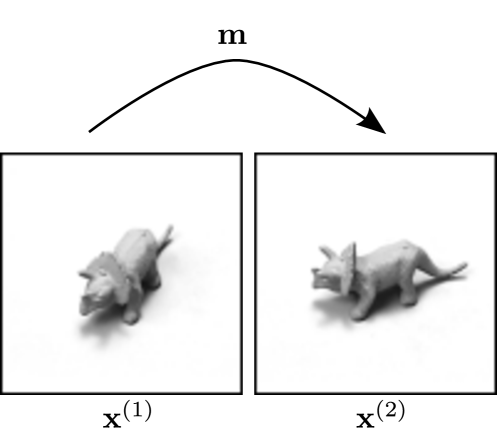
In a video, given one frame $\mathbf{x}^{(1)}$ there can be a multitude of potential next frames $\mathbf{x}^{(2)}$. It is therefore common to use bi-linear models, like the Gated Boltzmann Machine (GBM) Taylor & Hinton (2009), the Gated Autoencoder (GAE) Memisevic (2011), and similar models (see Memisevic, 2013, for an overview) whose hidden variables can represent which transformation, out of the pool of many possible transformations, can take $\mathbf{x}^{(1)}$ to $\mathbf{x}^{(2)}$.

More formally, bi-linear models learn to represent the linear transformation, $\mathbf{L}$, between two images $\mathbf{x}^{(1)}$ and $\mathbf{x}^{(2)}$, where

$$\mathbf{x}^{(2)}=\mathbf{L}\mathbf{x}^{(1)}$$ (1)

It can be shown that a weighted sum of products of filter responses is able to identify the transformation. The reason is that the weighted sum is large if the angle between filters is similar to the angle (in “pixel-space”) between the two frames. That way, hidden units represent the observed transformation in the form of a set of phase-differences in the invariant subspaces of the transformation class Memisevic (2013). As hidden units encode the transformation between images, rather than the content of the images, they are commonly referred to as mapping units. We shall focus on the autoencoder variant of these models for the purposes of this paper, but one can use other models such as the GBM.

Figure 2: Graphical representation of the gated autoencoder. The two inputs $\mathbf{x}^{(1)}$ and $\mathbf{x}^{(2)}$ are projected onto features and the mapping units pool over pairwise products of these features.

Formally, the response of a mapping unit layer can be written

$$\mathbf{m}=\sigma\big{(}\mathbf{W}{}(\mathbf{U}\mathbf{x}^{(1)}\odot\mathbf{V}{}\mathbf{x}^{(2)})\big{)}$$ (2)

where $\mathbf{U},\mathbf{V}{}$ and $\mathbf{W}{}$ are parameter matrices, and where $\odot$ denotes elementwise multiplication. Further, $\sigma$ is an elementwise non-linearity, such as the logistic sigmoid.

Given mapping unit activations, $\mathbf{m}$, as well as the first image, the second image can be reconstructed by applying the transformation encoded in $\mathbf{m}$ as follows Memisevic (2011):

$$\tilde{\mathbf{x}}{}^{(2)}=\mathbf{V}{}^{\mathrm{T}}\big{(}\mathbf{U}\mathbf{x}^{(1)}\odot\mathbf{W}{}^{\mathrm{T}}\mathbf{m}\big{)}.$$ (3)

As the model is symmetric, we can likewise define the reconstruction of the first image given the second as:

$$\tilde{\mathbf{x}}{}^{(1)}=\mathbf{U}^{\mathrm{T}}\big{(}\mathbf{V}{}\mathbf{x}^{(2)}\odot\mathbf{W}{}^{\mathrm{T}}\mathbf{m}\big{)}$$ (4)

from which one obtains the reconstruction error

$$\mathcal{L}=||\mathbf{x}^{(1)}-\tilde{\mathbf{x}}{}^{(1)}||^{2}+||\mathbf{x}^{(2)}-\tilde{\mathbf{x}}{}^{(2)}||^{2}$$ (5)

for training. It can be shown that minimizing reconstruction error on image pairs will turn each row in $\mathbf{U}$ and the corresponding row in $\mathbf{V}{}$ into a pair of phase-shifted filters. Together the filters span the invariant subspaces of the transformation class inherent in the training pairs with which the model was trained. As as result, each component of $\mathbf{m}$ is tuned to a phase-delta after learning, and it is independent of the absolute phase of each image Memisevic (2013).

3 Higher-order relational features

3.1 Approximating discrete-time dynamical systems

A quite natural extension of the concept of relational features can be motivated by looking at relational models as performing a kind of first-order Taylor approximation of the input sequence, where the hidden representation models the partial first-order derivatives of the inputs with respect to time. Based on this view, we propose an approach that exploits correlations between subsequent sequence elements to model a dynamical system which approximates the sequence. This is a very different way to address long-range correlations than assuming memory units that explicitly keep state Hochreiter & Schmidhuber (1997). Instead, here we assume that there is structure in the temporal evolution of the input stream and we focus on capturing this structure.

As an intuitive example, consider a video that is known to be a sinusoidal signal, but with unkown frequency, phase and motion direction. The complete video can be specified exactly and completely by the first three seed images. Therefore, given these three images, we would in principle be able to predict the rest of the video ad infinitum.

The first-order partial derivative of a multidimensional discrete-time dynamical system describes the correspondences between state vectors at subsequent time steps. Relational feature learning applied to subsequent elements of a sequence can be viewed as a way to learn these derivatives, suggesting that we may model higher-order partial derivatives with higher-order relational features.

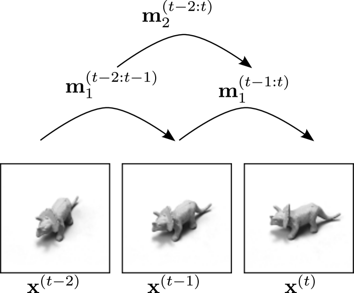
We model second-order derivatives by cascading relational features in a pyramid as depicted in 3. Given a sequence of inputs $\mathbf{x}^{(t-2)},\mathbf{x}^{(t-1)},\mathbf{x}^{(t)}$, first-order relational features ${\mathbf{m}_{1}^{(t-1:t)}}$ describe the transformations between two subsequent inputs $\mathbf{x}^{(t-1)}$ and $\mathbf{x}^{(t)}$. Second-order relational features ${\mathbf{m}_{2}^{(t-2:t)}}$ describe correspondences between two first-order relational features ${\mathbf{m}_{1}^{(t-2:t-1)}}$ and ${\mathbf{m}_{1}^{(t-1:t)}}$, modeling the analog of the partial second-order derivatives of the inputs with respect to time. Section 5.3 presents experiments with two layers of relational features that support this view.

Figure 3: First-order relational features ${\mathbf{m}_{1}^{(t-2:t-1)}}$ and ${\mathbf{m}_{1}^{(t-1:t)}}$ describe correspondences between multiple entities, e.g. two frames of a video. The second-order relational features ${\mathbf{m}_{2}^{(t-2:t)}}$ describe correspondences between the first-order relational features.

3.2 The higher-order gated autoencoder

We implement a higher-order gated autoencoder (HGAE) using the following modular approach. The second-order HGAE is constructed using two GAE modules, one that relates inputs and another that relates mappings of the first GAE.

The first-layer GAE instance models correspondences between input pairs using filter matrices $\mathbf{U}_{1},\mathbf{V}_{1}$ and $\mathbf{W}_{1}$ (the subscript index refers to the layer). Using the first-layer GAE, mappings ${\mathbf{m}_{1}^{(t-2:t-1)}}$ and ${\mathbf{m}_{1}^{(t-1:t)}}$ for overlapping input pairs $(\mathbf{x}^{(t-2)},\mathbf{x}^{(t-1)})$ and $(\mathbf{x}^{(t-1)},\mathbf{x}^{(t)})$ are inferred and this pair of first-layer mappings is used as input for a second GAE instance. This second GAE models correspondences between the mappings of the first-layer using filter matrices $\mathbf{U}_{2},\mathbf{V}_{2}$ and $\mathbf{W}_{2}$.

For the two-layer model, inference amounts to computing first- and second-order mappings according to

$${\mathbf{m}_{1}^{(t-2:t-1)}}=\sigma\big{(}\mathbf{W}_{1}\big{(} (\mathbf{U}_{1}\mathbf{x}^{(t-2)})\odot(\mathbf{V}_{1}\mathbf{x}^{(t-1)})\big{)}\big{)}$$ (6)

$${\mathbf{m}_{1}^{(t-1:t)}}=\sigma\big{(}\mathbf{W}_{1}\big{(} (\mathbf{U}_{1}\mathbf{x}^{(t-1)})\odot(\mathbf{V}_{1}\mathbf{x}^{(t)})\big{)}\big{)}$$ (7)

$${\mathbf{m}_{2}^{(t-2:t)}}=\sigma\big{(}\mathbf{W}_{2}\big{(} (\mathbf{U}_{2}{\mathbf{m}_{1}^{(t-2:t-1)}})\odot(\mathbf{V}_{1}{\mathbf{m}_{1}^{(t-1:t)}})\big{)}\big{)}$$ (8)

Cascading GAE modules in this way can also be motivated from the perspective of orthogonal transformations as subspace rotations. As stated in Memisevic (2013), summing over filter-response products can yield transformation detectors which are invariant to the initial phase of the transformation and also partially invariant to the content of the images. The relative rotation angle (phase delta) between two projections is itself an angle, and their relation can be viewed as an “angular acceleration”.

In contrast to the standard two-frame model, in this model reconstruction error is not directly applicable (although a naive way to train the model is to minimize reconstruction error for each pair of adjacent nodes in each layer). However, there is a more natural way to train the model if training data forms a sequence, as we discuss next.

4 Predictive training of relational models

4.1 Single-step prediction

Given the first two frames of a sequence $\mathbf{x}^{(1)},\mathbf{x}^{(2)},\mathbf{x}^{(3)}$ one can use the GAE to compute a prediction of the third frame as follows. First, mappings ${\mathbf{m}^{(1,2)}}$ are inferred from $\mathbf{x}^{(1)}$ and $\mathbf{x}^{(2)}$ (see Equation 2) and then used to compute a prediction $\hat{\mathbf{x}}{}^{(3)}$ by applying the inferred transformation ${\mathbf{m}^{(1,2)}}$ to frame $\mathbf{x}^{(2)}$. Applying the transformation amounts to computing:

$$\hat{\mathbf{x}}{}^{(3)}=\mathbf{V}{}^{\mathrm{T}}\big{(}\mathbf{U}\mathbf{x}^{(2)}\odot\mathbf{W}{}^{\mathrm{T}}{\mathbf{m}^{(1,2)}}\big{)}$$ (9)

This prediction of $\mathbf{x}^{(3)}$ will be a good prediction under the assumption that the frame-to-frame transformations from $\mathbf{x}^{(1)}$ to $\mathbf{x}^{(2)}$ and from $\mathbf{x}^{(2)}$ to $\mathbf{x}^{(3)}$ are approximately the same, in other words if transformations themselves are assumed to be approximately constant in time.

In this case, one can train the GAE to minimize the prediction error

$$\mathcal{L}=||\hat{\mathbf{x}}{}^{(3)}-\mathbf{x}^{(3)}||_{2}^{2}$$ (10)

instead of minimizing the reconstruction error in Equation 5. This type of supervised training objective, in contrast to the standard GAE objective, can also guide the mapping representation to be invariant to image content, because encoding the content of $\mathbf{x}^{(2)}$ will not in general help predicting $\mathbf{x}^{(3)}$.

Figure 4: The assumption of similarity between the transformations from $\mathbf{x}^{(t-1)}$ to $\mathbf{x}^{(t)}$ and from $\mathbf{x}^{(t)}$ to $\mathbf{x}^{(t+1)}$ allows us to define a prediction $\hat{\mathbf{x}}{}^{(t+1)}$ by applying the inferred transformation ${\mathbf{m}^{(t-1:t)}}$ to $\mathbf{x}^{(t)}$.

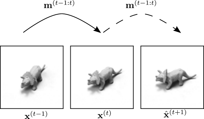
When the assumption of constancy of the transformations is violated, we can use a higher layer to model how transformations themselves change over time. This will require a farther look-ahead for predictive training which we discuss in the following.

4.2 Multi-step prediction

One can iterate the inference-prediction process to look more than one frame ahead in time. To compute a prediction $\hat{\mathbf{x}}{}^{(4)}$ one infers mappings from $\mathbf{x}^{(2)}$ and $\hat{\mathbf{x}}{}^{(3)}$:

$${\mathbf{m}^{(2:3)}}=\sigma\big{(}\mathbf{W}{}(\mathbf{U}\mathbf{x}^{(2)}\odot\mathbf{V}{}\hat{\mathbf{x}}{}^{(3)})\big{)}$$ (11)

and computes the prediction

$$\hat{\mathbf{x}}{}^{(4)}=\mathbf{V}{}^{\mathrm{T}}\big{(}\mathbf{U}\mathbf{x}^{(3)}\odot\mathbf{W}{}^{\mathrm{T}}{\mathbf{m}^{(2:3)}}\big{)}.$$ (12)

Then mappings can be inferred again from $\hat{\mathbf{x}}{}^{(3)}$ and $\hat{\mathbf{x}}{}^{(4)}$ to compute a prediction of $\hat{\mathbf{x}}{}^{(5)}$, and so on.

For the two-layer HGAE this amounts to the assumption that the second-order relational structure in the sequence changes slowly over time and under this assumption we compute a prediction $\hat{\mathbf{x}}{}^{(t+1)}$ in two steps: First a prediction is made of the first-order relational features describing the correspondence between $\mathbf{x}^{(t)}$ and $\mathbf{x}^{(t+1)}$:

$${\hat{\mathbf{m}}_{1}^{(t:t+1)}}={\mathbf{V}_{2}}^{\mathrm{T}}\big{(}\mathbf{U}_{2}{\mathbf{m}_{1}^{(t-1:t)}}\odot\mathbf{W}_{2}^{\mathrm{T}}{\mathbf{m}_{2}^{(t-2:t)}}\big{)}$$ (13)

Using this prediction of the transformation between $\mathbf{x}^{(t)}$ and $\mathbf{x}^{(t+1)}$ the prediction $\hat{\mathbf{x}}{}^{(t+1)}$ is made as follows:

$$\hat{\mathbf{x}}{}^{(t+1)}={\mathbf{V}_{1}}^{\mathrm{T}}\big{(}\mathbf{U}_{1}\mathbf{x}^{(t)}\odot\mathbf{W}_{1}^{\mathrm{T}}{\hat{\mathbf{m}}_{1}^{(t:t+1)}}\big{)}$$ (14)

Figure 5: A prediction is made in two steps (the dashed lines) from top-to-bottom. The second-order relational feature ${\mathbf{m}_{2}^{(t-2:t)}}$, inferred on the sequence $\mathbf{x}^{(t-2)},\mathbf{x}^{(t-1)},\mathbf{x}^{(t)}$ is assumed to be slowly changing and used to make a prediction of the first-order relational feature which describes the correspondences between $\mathbf{x}^{(t)}$ and $\mathbf{x}^{(t+1)}$. This prediction is then used to transform $\mathbf{x}^{(t)}$ into the prediction $\hat{\mathbf{x}}{}^{(t+1)}$.

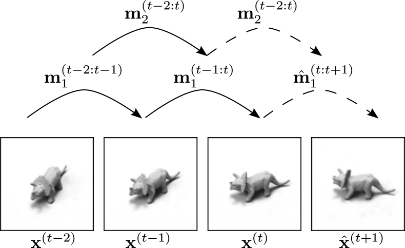
As with the GAE, one can predict multiple steps ahead in time using the HGAE by repeating the inference-prediction process on $\mathbf{x}^{(t-1)},\mathbf{x}^{(t)}$ and $\hat{\mathbf{x}}{}^{(t+1)}$, i.e. by appending the prediction to the sequence and increasing $t$ by one.

The prediction process simply consists of iteratively computing predictions of the next lower level’s activations beginning from the top. To compute the top-level activations themselves, one needs a number of seed frames corresponding to the depth of the model. While two frames are sufficient to infer the transformations in the case of the GAE, three frames are required in the case of the two-layer model.

The models can be trained using backprop through time Werbos (1988) to compute the gradients of the $k$-step ahead prediction error w.r.t. the parameters:

$$\mathcal{L}=\sum\limits_{i=1}^{k}||\hat{\mathbf{x}}{}^{(t+i)}-\mathbf{x}^{(t+i)}||_{2}^{2}$$ (15)

In our experiments, we observed that starting with single-step prediction, training and iteratively increasing the number of prediction steps during training considerably stabilizes the dynamics of the model and helps to prevent explosions in the magnitude of the predictions.

5 Experiments

We tested and compared the models on videos with varying degrees of complexity, from synthetic constant to synthetic accelerated transformations to more complex real-world transformations.

5.1 Preprocessing and initialization

For all data sets PCA whitening was used for dimensionality reduction, retaining around $95\%$ of the variance.

Predictive training of the HGAE only worked after layerwise pre-training. We used gradient descent with a learning rate of $0.001$ and momentum $0.9$. Without pretraining the parameters did not converge to a useful configuration. The first-layer GAE was trained to reconstruct pairs of subsequent sequence elements (as described in Section 2). Then pairs of mappings were computed on three subsequent inputs using the pretrained first-layer GAE. These mapping pairs were then used for reconstructive pretraining of the second-layer GAE.

5.2 Comparison of predictive and reconstructive training

(a) AccRot

(b) AccShift

(c) Bouncing Balls

(d) NORBVideos

Figure 6: HGAE first-layer filter pairs (after multi-step predictive training).

To evaluate whether predictive training of the GAE yields better representations of transformations than training with the reconstruction objective, a classification experiment on videos showing artificially transformed natural images was performed. The $13\times 13$ patches were cropped from the Berkeley Segmentation data set Martin et al. (2001). Two data sets with videos featuring constant velocity shifts ( ConstShift) and rotations (ConstRot) were generated. The elements of the shift vectors for the ConstShift data set were sampled uniformly from the interval $[-3,3]$ (in pixels). The rotation angles were sampled uniformly from the interval $(-\pi,\pi)$. Labels for the ConstShift data set were generated by dividing the shift vectors as shown in Figure 7. For ConstRot the angles were divided into $8$ equally-sized bins. Both data sets were partitioned into a training set containing $100\,000$, a validation set containing $20\,000$ and a test set containing $50\,000$ sequences.

The numbers of filters and mapping units were chosen using a grid search. The setting with best performance on the validation set was $256$ filters and $256$ mapping units each for both training objectives and both data sets. The models were each trained for $1\,000$ epochs using stochastic gradient descent (SGD) with a learning rate of $0.001$ and momentum $0.9$. For the experiment the mappings of the first two inputs were used as input to a logistic regression classifier. The experiment was performed multiple times on both data sets and the mean classification accuracies are reported in Table 1. In all trials the GAE trained with $1$-step predictive training achieved a higher accuracy than the GAE trained on the reconstruction objective. This suggests that predictive training is able to generate a more explicit representation of transformations, that is plagued less by image content, as discussed in Section 4.1.

Figure 7: Discretization of shift vectors: The 2D plane is divided into the four quadrants and then a magnitude threshold $\beta$ is chosen, such that the distribution of samples into the 8 shown bins (numbered $0-7$) is uniform. $\alpha$ denotes the maximum magnitude in the respective data set.

Table 1: Classification accuracy of the GAE on the constant rotations (ConstRot) and constant shifts (ConstShift) data sets, for reconstructive and $1$-step predictive training.

Model	ConstRot	ConstShift
rec. training	97.6	76.4
pred. training	98.2	79.4

5.3 Detecting acceleration

To test the hypothesis that the HGAE learns to model second-order correspondences in sequences, image sequences with accelerated shifts (AccShift) and rotations (AccRot) of natural image patches were generated. The patches were again cropped from the Berkeley Segmentation data set and artificially transformed with initial (angular) velocity and constant (angular) acceleration. The scalar angular accelerations were sampled uniformly from the interval $[-\frac{\pi}{12},\frac{\pi}{12}]$ degrees. The initial angular velocites were sampled from the same interval. To get labels for classification, the angular accelerations were divided into $8$ equally sized bins. For the accelerated shifts data set, elements of the velocity and acceleration vectors were sampled in the interval $[-3,3]$ (in pixels). The discretization of acceleration vectors is the same as for the shift vectors in ConstShift (see Figure 7). The partition sizes are the same as for ConstRot and ConstShift.

The number of filters and mapping units was set to $512$ and $256$, respectively (after performing a grid search). After pretraining the HGAE was trained with gradient descent using a learning rate of $0.0001$ and momentum of $0.9$, first for $400$ epochs on single-step prediction and then $500$ epochs on two-step prediction.

After training, first- and second-layer mappings were inferred from the first three frames of the test sequences. The classification accuracies using logistic regression with second-layer mappings of the HGAE (${\mathbf{m}_{2}^{(1:3)}}$) as descriptor, using the individual first-layer mappings (${\mathbf{m}_{1}^{(1:2)}}$ and ${\mathbf{m}_{1}^{(2:3)}}$), and using the concatenation of both first-layer mappings are reported in Table 2 for both data sets (before and after predictive finetuning).

Table 2: Classification accuracies (%) using different layer mappings of the HGAE before and after 2-step finetuning on the accelerated rotations (AccRot) and the accelerated shifts (AccShift) data set. $({\mathbf{m}_{1}^{(1:2)}},{\mathbf{m}_{1}^{(2:3)}})$ denotes the concatenation of both first-layer mappings.

	Descriptor	AccRot	AccShift
pretrained	${\mathbf{m}_{1}^{(1:2)}}$	19.4	20.6
	${\mathbf{m}_{1}^{(2:3)}}$	30.9	33.3
	$({\mathbf{m}_{1}^{(1:2)}},{\mathbf{m}_{1}^{(2:3)}})$	64.9	38.4
	${\mathbf{m}_{2}^{(1:3)}}$	53.7	63.4
finetuned	${\mathbf{m}_{1}^{(1:2)}}$	18.1	20.9
	${\mathbf{m}_{1}^{(2:3)}}$	29.3	34.4
	$({\mathbf{m}_{1}^{(1:2)}},{\mathbf{m}_{1}^{(2:3)}})$	74.0	42.7
	${\mathbf{m}_{2}^{(1:3)}}$	74.4	80.6

Figure 8: Two examples for seven prediction steps of the HGAE model on the AccRot data set, shown are from top to bottom, groundtruth, the predictions of the model after pretraining, and after one-, two- and three-step predictive training.

Figure 9: Two examples of predictions using the HGAE model on the AccShift data set, shown are from top to bottom, groundtruth, the predictions of the model after pretraining, one- and two-step predictive training.

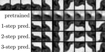
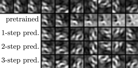
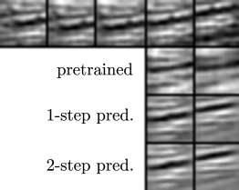
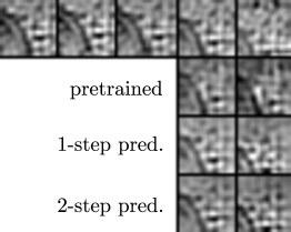
The second-layer mappings achieved a significantly higher accuracy for both data sets after predictive training. For the AccRot data set, the concatenation of first-layer mappings performed better than the second-layer mappings before finetuning, which may be because the angular acceleration data is based on a one-parameter transformation and is thus simpler than the shift acceleration data, which is based on a two-parameter transformation. Predictive finetuning also helped improve the intermediate representation, as can be observed by the increase in accuracy for the concatenation of the first-layer mappings.

These results shows that the second layer of the HGAE can build a much better representation of the second-order relational structure in the data than the single-layer GAE model. They further show that predictive training improves the capability of both models and is crucial for the two-layer model to work well.

5.4 Sequence prediction

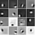
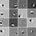
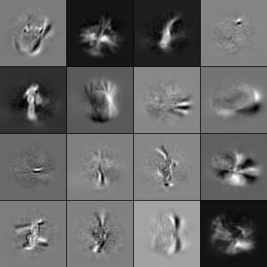
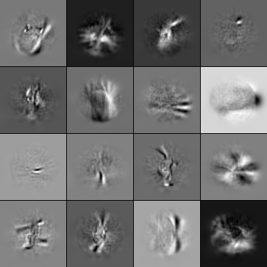
In this experiment we test the capability of the models to predict previously unseen sequences multiple steps into the future. This allows us to assess to what degree modeling second order “derivatives” makes it possible to capture the temporal evolution without resorting to an explicit representation of a hidden state. After training, test sequences were generated by seeding the models with two (GAE) or three (HGAE) seed frames. Figure 6 shows some of the filter pairs learned by the HGAE on different data sets after predictive training.

5.4.1 Accelerated transformations

Figures 8 and 9 show predictions with the HGAE model on the data sets introduced in Section 5.3 after different stages of training. As can be seen in the figures, the accuracy of the predictions increases significantly with multi-step training.

5.4.2 NorbVideos

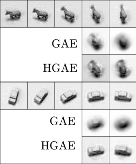
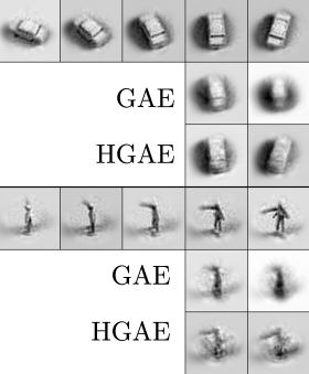
The NORBvideos data set introduced in Memisevic & Exarchakis (2013) contains videos of objects from the NORB dataset LeCun et al. (2004). These are objects divided into $5$ classes (four-legged animals, human figures, airplanes, trucks and cars), each with $9$ instances. The $5$ frames of each video from the NORBvideos data show incrementally changed viewpoints of one of the objects. We trained our sequence learning models on this data, using the author’s original split: all videos of objects from instances $1-8$ are in the training set and instance $9$ objects are in the test set. This yields $109\,350$ training examples and $12\,150$ test examples. The frame size is $96\times 96$ and the videos are $5$ frames long. The GAE and the HGAE model were trained on the multi-step prediction task with a learning rate of $0.0001$ and momentum $0.9$. Both models used $2000$ features and $1000$ mapping units (per layer). The test-performance of the GAE model seemed to stop improving at $2000$ features, while the HGAE was able to make use of the additional parameters.

Figure 10 shows predictions made by both models. The HGAE manages to generate predictions that correctly reflect the 3-D structure in the data. In contrast to the GAE model it is much better at extrapolating the observed transformations. Note that seed frames are from test data.

Due to the large input dimensionality and the low number of training samples a few of the filters shown in Figure 6(d) seem to be overfitting on the training data while many others are localized Gabor-like features.

5.4.3 Bouncing Balls

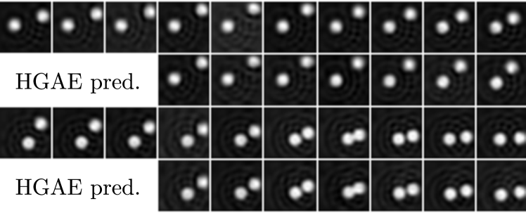
We also trained the HGAE on the bouncing balls data set to see whether the HGAE captures the highly non-linear dynamics of this data set. The number of features was set to $512$ and the number of mappings to $256$. Figure 11 shows two predictions on test data. The predictions show that the second-order model is able to correctly capture reflections on the boundaries and the other balls, and makes consistent predictions over in some cases up to around $10-20$ frames.

Figure 10: Comparison of 10 prediction steps on the NORBvideos data set. The original sequences only contain $5$ frames, providing only 2 frames of ground truth for predictions.

Figure 11: Seven HGAE prediction steps on two samples of the bouncing balls data set after training on 3-step predictions.

6 Discussion

A major long-standing problem in sequence modeling is how to deal with long range correlations. It has been proposed that deep learning may help address this problem by finding representations that capture better the abstract, semantic content of the inputs Bengio (2009). In this work we propose learning representations with the explicit goal to enable the prediction of the temporal evolution of the input stream multiple time steps ahead. Thus we seek a hidden representation that captures exactly those aspects of the input data which allow us to make predictions about the future.

It is interesting to note that predictive training can also be viewed as an analogy making task Memisevic & Hinton (2010). It amounts to taking the transformation taking frame $t$ to $t+1$ and applying it to a new observation at time $t+1$ or later. The difference is that in a genuine analogy making task, the target image may be unrelated to the source image pair, whereas here target and source are related. It would be interesting to apply the model to word representations, or language in general, as this is a domain where both, sequentially structured data and analogical relationships between data-points, play a crucial role (e.g. Mikolov et al., 2013).

References

- Bengio (2009) Bengio, Yoshua. Learning deep architectures for AI. Foundations and Trends in Machine Learning, 2(1):1–127, 2009. Also published as a book. Now Publishers, 2009.
- Hochreiter & Schmidhuber (1997) Hochreiter, Sepp and Schmidhuber, Jürgen. Long short-term memory. Neural computation, 9(8):1735–1780, 1997.
- LeCun et al. (2004) LeCun, Yann, Huang, Fu Jie, and Bottou, Leon. Learning methods for generic object recognition with invariance to pose and lighting. In Computer Vision and Pattern Recognition, 2004. CVPR 2004. Proceedings of the 2004 IEEE Computer Society Conference on, volume 2, pp. II–97. IEEE, 2004.
- Martin et al. (2001) Martin, D., Fowlkes, C., Tal, D., and Malik, J. A database of human segmented natural images and its application to evaluating segmentation algorithms and measuring ecological statistics. In Proc. 8th Int’l Conf. Computer Vision, volume 2, pp. 416–423, July 2001.
- Memisevic & Hinton (2010) Memisevic, R. and Hinton, G.E. Learning to represent spatial transformations with factored higher-order boltzmann machines. Neural Computation, 22(6):1473–1492, 2010.
- Memisevic (2011) Memisevic, Roland. Gradient-based learning of higher-order image features. In Computer Vision (ICCV), 2011 IEEE International Conference on, pp. 1591–1598. IEEE, 2011.
- Memisevic (2013) Memisevic, Roland. Learning to relate images. IEEE Transactions on Pattern Analysis and Machine Intelligence, 35(8):1829–1846, 2013.
- Memisevic & Exarchakis (2013) Memisevic, Roland and Exarchakis, Georgios. Learning invariant features by harnessing the aperture problem. In Proceedings of the 30th International Conference on Machine Learning (ICML 2013), 2013.
- Memisevic & Hinton (2007) Memisevic, Roland and Hinton, Geoffrey. Unsupervised learning of image transformations. In Proceedings of IEEE Conference on Computer Vision and Pattern Recognition, 2007.
- Mikolov et al. (2013) Mikolov, Tomas, Chen, Kai, Corrado, Greg, and Dean, Jeffrey. Efficient estimation of word representations in vector space. CoRR, abs/1301.3781, 2013.
- Sutskever et al. (2008) Sutskever, Ilya, Hinton, Geoffrey E, and Taylor, Graham W. The recurrent temporal restricted boltzmann machine. In Advances in Neural Information Processing Systems, pp. 1601–1608, 2008.
- Sutskever et al. (2011) Sutskever, Ilya, Martens, James, and Hinton, Geoffrey. Generating text with recurrent neural networks. In Proceedings of the 2011 International Conference on Machine Learning (ICML-2011), 2011.
- Taylor & Hinton (2009) Taylor, Graham and Hinton, Geoffrey. Factored conditional restricted Boltzmann machines for modeling motion style. In Proceedings of the 26th International Conference on Machine Learning, Montreal, June 2009. Omnipress.
- Werbos (1988) Werbos, Paul J. Generalization of backpropagation with application to a recurrent gas market model. Neural Networks, 1(4):339–356, 1988.