A new paradigm for petascale Monte Carlo simulation: Replica exchange Wang–Landau sampling

Abstract

We introduce a generic, parallel Wang–Landau method that is naturally suited to implementation on massively parallel, petaflop supercomputers. The approach introduces a replica-exchange framework in which densities of states for overlapping sub-windows in energy space are determined iteratively by traditional Wang–Landau sampling. The advantages and general applicability of the method are demonstrated for several distinct systems that possess discrete or continuous degrees of freedom, including those with complex free energy landscapes and topological constraints.

1 Introduction

One of the great challenges accompanying recent developments in high performance computing hardware is the question of how to make truly efficient use of the huge numbers of cores found in today’s “cutting edge” machines. There have been concomitant developments in methodology in computational statistical physics, one of the most recent of them being a parallel implementation of the very successful importance sampling Monte Carlo based approach termed “Wang–Landau sampling” [1]. In the original Wang–Landau sampling, the a priori unknown density of states $g(E)$ of a system is determined iteratively by performing a random walk in energy space ($E$) and sampling configurations with probability $1/g(E)$ (i.e. with a “flat histogram”) [2, 3, 4]. Many studies have shown that this procedure is very powerful for studying a number of diverse problems including those with complex free energy landscapes because it circumvents the very long time scales encountered near phase transitions or at low temperatures. The method also facilitates the direct calculation of thermodynamic quantities, including the free energy, at any temperature from a single simulation. (In fact, random walks in the space of more than one variable allow thermodynamic information to be determined as a function of more than one thermodynamic field from a single simulation.) Wang–Landau sampling is also a generally applicable Monte Carlo procedure with only a few adjustable parameters, and it has been applied successfully to a wide range of simulation models, some with discrete degrees of freedom and some involve degrees of freedom that are continuous (see [5, 6, 7, 8] for examples). While modifications to the initial implementation have been proposed, e.g. by optimizing the “modification factor–flatness criterion” scheme [9, 10, 11], by introducing more efficient Monte Carlo trial moves [12, 13, 14], or “error correction” [15], the underlying simplicity has remained intact. Thus, the basic algorithm is an excellent candidate for parallel implementation.

A few simple attempts at parallelizing Wang–Landau sampling have been implemented, but these are useful only for a relatively small number of processors (cores). One early approach [3, 4] subdivided the total energy range into smaller sub-windows, each being sampled by an independent random walker. The total simulation time needed is then limited by the convergence of the slowest walker, but this can be tuned by an unequal partition of energy space. Nevertheless, “perfect” load balancing is impossible due to the a priori unknown nature of the complex free energy landscape. Furthermore, the individual energy sub-windows cannot be reduced arbitrarily in range because some regions of configurational space would then ultimately become inaccessible. In another approach to parallelization, multiple random walkers work simultaneously on the same density of states and histogram. Distributed memory (MPI [16]), shared memory (OpenMP [17], multi-thread [18]), and GPU [19] variants of this idea have been proposed; shared memory implementations have the advantage of not requiring periodic synchronization among the walkers and even allow for “data race” when updating $g(E)$ without noticeable loss in accuracy [17]. Although this second approach would appear to avoid the problems of the first approach, a recent, massively parallel implementation [19] found that correlations among the walkers could lead to a systematically underestimation of $g(E)$ in “difficult to access”, low energy regions. The addition of a phenomenological bias to the modification factor alleviated this difficulty, the effective round-trip times of the individual walkers, however, are not improved through the use of this ”ad hoc” method and the validity of the approach cannot be confirmed.

2 The new, parallel (replica exchange Wang–Landau) algorithm

Our new approach [1, 20] is a generic, parallel Wang–Landau scheme which combines the benefits of the original Wang–Landau (WL) sampling scheme with those of replica-exchange Monte Carlo [21, 22, 23]. Much of the success of the Wang–Landau algorithm has resulted from the combination of its simplicity and robustness, and our goal was to retain these qualities in the parallel algorithm. We begin by splitting up the total energy range into smaller, overlapping sub-windows. Sampling then proceeds in each energy sub-window by multiple, independent Wang–Landau walkers, each of which has its own instantaneous density of states and histogram. The key to this approach is that configurational, or replica, exchanges are allowed between walkers in overlapping energy sub-windows during the simulation. Consequently, each replica can travel back and forth over the entire energy space many times during a single simulation. The replica exchange move does not bias the overall procedure; thus the approach is applicable with any valid trial update or Wang–Landau convergence criterion (e.g., the “$1/t$ algorithm” [11]). Furthermore, the parallel algorithm does not impose any intrinsic limitation to the number of random walkers and the number of energy sub-windows that can grow with the size of the system. Therefore, the computational method should scale straightforwardly to many thousands of cores.

The standard Wang–Landau algorithm [2, 3] estimates the density of states, $g(E)$, using a single random walker in an energy range $\left[E_{\mathrm{min}},E_{\mathrm{max}}\right]$. During the simulation, trial moves are accepted with a probability $P=\textrm{min}\left[1,g(E_{\mathrm{old}})/g(E_{\mathrm{new}})\right]$, where $E_{\mathrm{old}}$ ($E_{\mathrm{new}}$) is the energy of the original (proposed) configuration. The estimation of $g(E)$ is continuously adjusted and improved using a modification factor $f$ (i.e. $g(E)\to f\times g(E)$) which starts with $f_{0}>1$ and progressively approaches unity as the simulation proceeds. A histogram, $H(E)$, keeps track of the number of visits to each energy $E$ during a given iteration. When $H(E)$ is sufficiently “flat”, the next iteration begins with $H(E)$ reset to zero but keeping the estimate of $g(E)$ from the previous iteration, and $f$ reduced by some predefined rule (e.g. $f\rightarrow\sqrt{f}$). The simulation ends when $f$ reaches a sufficiently small value $f_{\mathrm{final}}$ at which point the accuracy of $g(E)$ is proportional to $\sqrt{f}_{\mathrm{final}}$ for sufficiently flat $H(E)$ [9].

Figure 1: a) Subdivision of the global energy range into nine equal-size intervals with overlap $o=75\%$. b) Run-time balanced subdivision with overlap to the higher energy interval $o\geq 75\%$. Multiple Wang–Landau walkers can be employed within each interval.

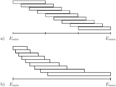
In our parallel Wang–Landau framework, the global energy range is first split into $h$ overlapping sub-windows, and $m$ random walkers are used to sample each sub-window. The extent of the overlap $o$ should strike a balance between fast convergence of $g(E)$ and a reasonable exchange acceptance rate. While an overlap of $o\approx 75\%$ works well, excellent results can be obtained with other values [20]. (Different types of partitioning of the global energy into sub-windows may be used; but, in all cases, configurational exchange cannot occur without overlap of adjacent sub-windows, see Fig. 1 for examples.) Within an energy sub-window, each random walker performs standard Wang–Landau sampling. After a predetermined number of Monte Carlo steps, a “replica exchange” is proposed between two random walkers, $i$ and $j$, where walker $i$ chooses swap partner $j$ from a neighboring sub-window at random. For the sake of simplicity and generality in our discussion, we do not sort out walkers which are currently not in the overlap region before drawing the pairs. Let $X$ and $Y$ be the configurations that the random walkers $i$ and $j$ are “carrying” before the exchange; $E(X)$ and $E(Y)$ be their energies, respectively. From the detailed balance condition the acceptance probability $P_{\mathrm{acc}}$ for the exchange of configurations $X$ and $Y$ between walkers $i$ and $j$ is:

$$P_{\mathrm{acc}}=\min\left[1,\frac{g_{i}(E(X))}{g_{i}(E(Y))}\frac{g_{j}(E(Y))}{g_{j}(E(X))}\right]\,$$ (1)

where $g_{i}(E(X))$ is the instantaneous estimator for the density of states of walker $i$ at energy $E(X)$, cf. [24]. Note that if either of the random walkers has an energy that lies outside the range of the sub-windows of the other, the replica exchange cannot take place. In that case, we just disregard the exchange and carry out another number of MC steps until the next replica exchange is proposed. This combination of sampling trials defines the new parallel algorithm.

An important new feature of our formalism is that each random walker has its own $g(E)$ and $H(E)$ which are updated independently. Also, since every walker has to satisfy the Wang–Landau flatness criterion independently at each iteration, the systematic errors found in [19] are avoided. When all random walkers within an energy sub-window have attained flat histograms, their estimates for $g(E)$ are averaged and then redistributed among themselves before simultaneously proceeding to the next iteration. This procedure reduces the error during the simulation with ${\sqrt{m}}$ [20], i.e. as for uncorrelated WL simulations. Furthermore, increasing $m$ can improve the convergence of the Wang–Landau sampling by reducing the risk of statistical outliers in $g(E)$ resulting in slowing down subsequent iterations. Alternatively, it allows us in principle, to use a weaker flatness criterion [20], which is in the spirit of a concurrently proposed idea of merging histograms in multicanonical simulations [25].

The parallel simulation ends when the modification factors in all the energy intervals have reached $f_{\mathrm{final}}$ and the $h\times m$ pieces of $g(E)$ fragments with overlapping energy sub-windows are then used to construct a single $g(E)$ over the entire energy range.

3 Data analysis and production run

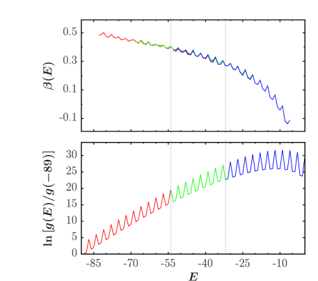
To connect two pieces of consecutive, overlapping density of states fragments, say $g_{i}(E)$ and $g_{j}(E)$, we first calculate the inverse microcanonical temperatures, $\beta_{i}(E)$ and $\beta_{j}(E)$ by: $\beta(E)=\textrm{d}\log[g(E)]/\textrm{d}E$. The joining point, $E_{\mathrm{join}}$, is determined as the point where $\Delta\beta=|\beta_{i}(E)-\beta_{j}(E)|$ vanishes or is the smallest. This procedure avoids discontinuities in the derivatives of the final density of states, which can lead to artificial peaks in derived functions like the heat capacity, for example. Next, $g_{j}(E)$ has to be rescaled using the value $g_{i}(E_{\mathrm{join}})$ as the reference point to yield a correct ratio for different energy levels: $g_{j}(E)\rightarrow g_{j}(E)(g_{i}(E_{\mathrm{join}})/g_{j}(E_{\mathrm{join}}))$. Finally, a joined relative density of states can be obtained by:

$$g(E)=\left\{\begin{array}[]{ll}g_{i}(E)&\textrm{if $E<E_{\mathrm{join}}$}\\ g_{j}(E)&\textrm{if $E\geq E_{\mathrm{join}}$}\,.\end{array}\right.$$ (2)

Here, we have assumed $j>i$ for Eq. (2) but this does not need to be the case for the previous rescaling procedure to work properly. See Fig. 2 for an illustration of the procedure described so far. Since there are $m$ pieces of density of states in each energy window, it is possible to compute the statistical errors by standard resampling techniques, e.g. jackknife or bootstrap methods, which can be found in standard textbooks. A more comprehensive discussion on this topic as applied to our data analysis scheme is presented in Ref. [20].

Figure 2: (color) Joining pieces of $g(E)$ for the HP 67mer adsorption on a weak attractive surface (Complete data shown in Fig. 5 a). (Top) First derivatives of raw DOS pieces from the three highest-energy windows. We applied a 5-point stencil with step-width $\Delta E=3$. Derivatives coincide best at $E=-54$ (red vs. green curve) and at $E=-32$ (green vs. blue curve; marked by vertical dotted lines). (Bottom) Pieces are connected at these points to obtain overall DOS.

Very often one is not only interested in obtaining a one-dimensional density of states, but a two-dimensional (or even higher dimensional) density of states, $g(E,Q)$, where $Q$ is a physical quantity. Such joint densities of states can be particularly useful for the calculation of thermodynamic properties of order parameters, for instance. One way of doing this is to perform a two-dimensional Wang–Landau sampling as proposed in the original treatment [2, 3, 4]; a more efficient way is to carry out a two-dimensional multicanonical production run using $1/g(E)$, obtained from a one-dimensional Wang–Landau sampling, as the simulation weight and construct $g(E,Q)$ from measurements of $E$ and $Q$ (see, for example, Ref. [26] for details).

In any case, one is confronted with the necessity of constructing the entire two-dimensional, joint density of states from fragments of $g(E,Q)$. We found that a direct generalization from the aforementioned one-dimensional scheme with a slight modification is able to yield satisfactory outcomes : let $g_{i}(E,Q)$ and $g_{j}(E,Q)$ be the two pieces of 2D density of states to be merged. We first calculate the normal vectors of the surfaces $S(E,Q)=\log\,g(E,Q)$:

$$\hat{N}=\left(\begin{array}[]{c}\partial S(E,Q)/\partial E\\[2.84526pt] \partial S(E,Q)/\partial Q\\[2.84526pt] -1\end{array}\right)\,,$$ (3)

from which the unit normal vectors $\hat{n}$ are calculated at all points $(E,Q)$. The joining position can then be determined as the point where these vectors best coincide, i.e., where $\hat{n_{i}}\cdot\hat{n_{j}}$ is maximal. One of the $g(E,Q)$ fragments is again rescaled in the same way as in the 1D case, and finally a joined relative density of states is determined by:

$$g(E,Q)=\left\{\begin{array}[]{cl}g_{i}(E,Q)&\textrm{if $(E,Q)$ is present only in window $i$}\\ g_{j}(E,Q)&\textrm{if $(E,Q)$ is present only in window $j$}\\ (g_{i}(E,Q)+g_{j}(E,Q))/2&\textrm{if $(E,Q)$ is present in both windows}\,.\end{array}\right.$$ (4)

This procedure is used for the analysis of our example models in Sect. 5.

4 Performance measures and scaling

In order to assess the generality and performance of this parallel Wang–Landau scheme, we applied it to multiple, fundamentally different models. As for most new computational schemes in statistical physics, we first tested our framework on the “fruit fly” of statistical physics, the Ising model. We simulated the 2D Ising model with system sizes as large as $256^{2}$ using more than 2000 cores. While single-walker Wang–Landau sampling typically takes more than a week to converge, the parallel scheme easily finishes within a few hours, with the same accuracy as the serial scheme. The deviations from the exact results are always of the same order as the statistical errors, which are $<0.01\%$ in the peak region of the density of states.

Figure 3: a) Dependence of the speed-up $s_{o}(h,m)$ on the number of energy windows and overlap $o=75\%$ (filled symbols, cf. Fig. 1 a) and using a run-time balanced energy splitting (open symbols, cf. Fig. 1 b). Here, the calculation of the speed-up is based on the MC steps (MCS) needed to complete the first WL iteration. Measurements are performed using the lipid bilayer system, see text for details.

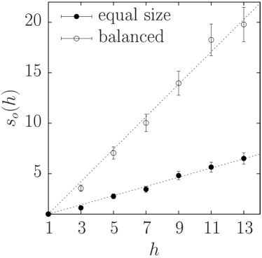
To generally quantify the efficiency of the parallel WL scheme, we define the speed-up, $s_{o}(h,m)$, as the number of Monte Carlo steps taken by the slowest parallel WL walker ($N_{o}^{\mathrm{parallel}}(h,m)$), as compared to that taken by a single walker ($N^{\mathrm{single}}$):

$$s_{o}(h,m)=\frac{N^{\mathrm{single}}}{N_{o}^{\mathrm{parallel}}(h,m)}.$$ (5)

We measure this number for $h\lesssim 20$ in simulations of the lipid system to be introduced below. As shown in Fig. 3, we find strong scaling, i.e. the speed-up scales linearly with $h$ for a fixed number $m$ for both energy splittings as shown in Fig. 1. While the equal-size energy range splitting (Fig. 1 a) is the most basic approach, the run-time balanced energy splitting (Fig. 1 b) is chosen such that walkers in different energy sub-windows complete the first WL iteration after the same number of MC sweeps (within statistical fluctuations). As the growth behavior of WL histograms is in principle known [9], such an energy splitting can be estimated by analyzing the first-iteration histogram from a short pre-run with equal-size energy intervals. We have shown in Ref. [1] that our method can also achieve weak scaling properties. With the capability of achieving both strong and weak scaling (i.e., by increasing the number of computing cores one can get results faster for the same system and/or simulate larger systems in the same period of time, respectively), our formalism becomes a promising candidate for large-scale applications.

5 Opening new vistas

To show how this parallel framework can allow us to examine previously unapproachable problems, we also applied the method to two very distinct and particularly challenging molecular systems: a coarse-grained continuum model for the self assembly of amphiphilic molecules (lipids) in explicit water and a discrete model for the surface adsorption of lattice proteins. In the first model, amphiphilic molecules, each of which is composed of a polar (P) head and two hydrophobic (H) tail monomers (P–H–H), are surrounded by solvent particles (W). The interactions between H and W molecules, as well as those between H and P molecules, are purely repulsive. All other interactions between non-bonded particles are of Lennard-Jones type; bonded molecules are connected by a FENE potential, see Refs. [29, 30] for similar models. The second model uses the hydrophobic-polar (HP) lattice model [31] for protein surface adsorption. Here a protein is represented by a self-avoiding walk consisting of H and P monomers placed on a simple cubic lattice with an attractive substrate. For recent simulational results on this model and computational details see [26, 32].

Figure 4: (color; Top) Logarithm of the density of states of the amphiphilic system containing 75 lipid molecules and a total of 1000 particles obtained by our parallel Wang–Landau scheme with the setup shown in Fig. 1 a. The pictures show a conformation where lipid molecules assemble and form a single cluster ($E\approx-2100$) and a low-energy bilayer configuration ($E\approx-4800$). (Bottom) Path of one single replica (out of 27 contributing to the above density of states) through energy space. Replica exchanges between walkers are proposed every $10^{4}$ sweeps (data also shown with that resolution), with acceptance rates between 30 and 55 %. Grid lines correspond to the borders of the individual energy windows.

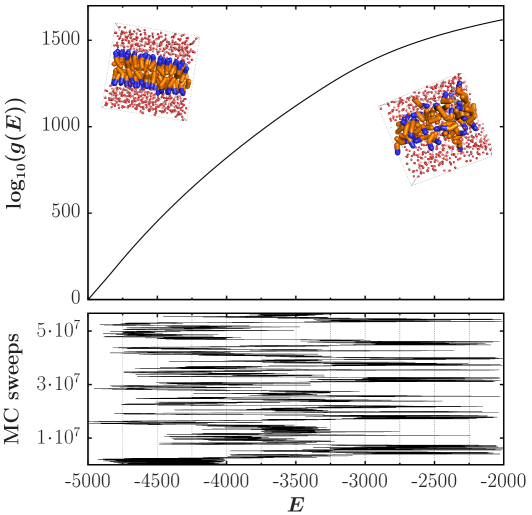
Both models pose technical challenges due to high energy and$/$or configurational barriers. Simulations of either setup is impossible for all practical purposes using the traditional, single walker Wang–Landau method due to unreasonable resource demands. (Standard Metropolis sampling would be many orders of magnitude too slow.) The first model (the amphiphilic system) consists of 75 lipid molecules (each composed of three particles) and 775 solution particles with a continuous energy domain. The density of states $g(E)$ over an energy range covering the lipid bilayer formation spans more than 1600 orders of magnitude, which makes precise low temperature properties extremely difficult to estimate. Only with the parallel algorithm, it is possible to clearly observe and study the lipid bilayer formation and different bilayer phases in this system. See Fig. 4 for example data and Refs. [27, 28] for all simulation details.

The second model (the HP lattice protein) under consideration consists of 67 monomers [33] interacting with a weakly attractive surface, for which the total energy of the system can be calculated as:

$$E=-(n_{HH}\varepsilon_{HH}+n_{SH}\varepsilon_{SH}+n_{SP}\varepsilon_{SP}),$$ (6)

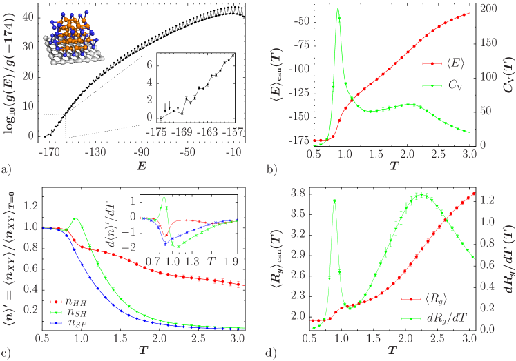
where $n_{HH}$, $n_{SH}$ and $n_{SP}$ are the number of hydrophobic interactions, surface-H interactions, and surface-P interactions, respectively; $\varepsilon_{HH}$, $\varepsilon_{SH}$ and $\varepsilon_{SP}$ are the corresponding energy scales. The discrete energy levels and the unequal interaction strengths between the H monomers and with the surface result in an unusual, sawtooth-like density of states, as shown in Fig. 5 a. This, combined with other obstacles such as the first-order like structural transitions in the system and the peculiar form of the density of states near the ground state, makes convergence for the entire energy range extremely time-consuming using only a single walker. Simulating smaller energy sub-windows individually as proposed by earlier studies was also not successful for this kind of system, due to the fact that too-small energy window would destroy ergodicity in the simulation. Consequently, some regions in the configurational space are unreachable, resulting in an incompletely simulated density of states.

However, we successfully simulated this model by our parallel Wang–Landau algorithm within a reasonable time frame. The density of states over the entire energy range and the thermodynamic properties of a few structural properties are shown in Fig. 5. From $g(E)$, the average energy $\langle E\rangle$ and the heat capacity $C_{V}$, both shown in Fig. 5 b, can be calculated:

$$\left\langle E\right\rangle =Z^{-1}\sum_{E}{Eg(E)e^{-E/k_{B}T}}\,,$$ (7)

$$C_{V} =\frac{\left\langle E^{2}\right\rangle-\left\langle E\right\rangle^{2}}{k_{B}T^{2}}\,,$$ (8)

where $Z=\sum_{E}{g(E)e^{-E/k_{B}T}}$ is the partition function at temperature $T$ with Boltzmann factor $k_{B}$.

To identify precisely which transitions are responsible for the peak at $T\approx 0.9$ and the shoulder across $T\approx 1.0$–$2.0$ in $C_{V}$, we compare it with the thermodynamics of the number of contacts between different particle species, i.e., the contributions to the total energy given in Eq. (6), and the radius of gyration, $R_{g}^{2}=\frac{1}{N}\sum_{i=1}^{N}{(\vec{r}_{i}-\vec{r}_{cm})^{2}}$, where $\vec{r}_{cm}$ is the center of mass of the configuration, $\vec{r}_{i}$ is the position of monomer $i$, and $N$ is the chain length. These results are shown in Fig. 5 c and d and were obtained through the joint density of states estimation as discussed earlier, where mean values are calculated via:

$$\langle Q\rangle=Z_{Q}^{-1}\sum_{E,Q}Q\,g(E,Q)\,e^{-E/k_{B}T}\,,$$ (9)

using the corresponding partition sum $Z_{Q}$.

From the derivative of the number of H–H contacts, $d\left\langle n_{HH}\right\rangle/dT$, we can see that the hydrophobic core formation occurs mainly at $T\approx 0.9$ and mildly at $T\approx 1.7$. By looking at the number of surface–H contacts, $d\left\langle n_{SH}\right\rangle/dT$, it is clear that adsorption is initiated by the attraction of the hydrophobic surface at $T\approx 1.1$. The polar monomers, although not attracted by the surface, are dragged to come in contact with the surface besides forming a polar shell of the protein. This causes a negative peak in $d\left\langle n_{SP}\right\rangle/dT$ at a lower temperature of $T\approx 0.9$. But recall that at the same temperature, the transition to ground state (hydrophobic core formation) is also taking place, which draws some H monomers from the surface to the core, resulting in a negative trough (visually, a peak) in $d\left\langle n_{SH}\right\rangle/dT$.

The radius of gyration and its derivative, shown in Fig. 5 d, give us extra information about the structural changes of the system. The peak at $T\approx 2.2$ in $d\langle R_{g}\rangle/dT$ signals the $\theta$-transition, where an extended coil collapses into a globular structure. This confirms the above observation on $d\left\langle n_{HH}\right\rangle/dT$, as it is necessary to first (i.e., at a higher temperature) bring the monomers closer together before the mild hydrophobic core formation can take place at $T\approx 1.7$. Another peak found at $T\approx 0.9$ is a more obvious reinforcement of our previous observation. During the transition to the ground state, there is a competition between the major hydrophobic core formation (which tends to decrease $R_{g}$ significantly) and adsorption (which tends to increase $R_{g}$ slightly), causing a large fluctuation in $R_{g}$. Since both the hydrophobic core formation and adsorption take place at nearly the same temperature, a single, pronounced peak is observed in $C_{V}$ eventually. This is a typical Category III transition according to the scheme defined in Ref. [26].

Figure 5: (color; a) Density of states of the lattice HP 67mer, where only H-monomers are attracted by the substrate. The H–H interaction is three times stronger than the surface attraction ($\varepsilon_{HH}=3$, $\varepsilon_{SH}=1$ and $\varepsilon_{SP}=0$), leading to the unusual sawtooth like shape. The inset shows the error bars on the enlarged low-energy data. Note the two energy gaps, i.e. no conformations exist with $E=-173$, $-172$, and $-170$ (see arrows). The picture shows an adsorbed HP protein with energy $E=-174$. (b) The corresponding canonical mean energy and heat capacity; (c) number of single H–H interactions and surface contacts; and (d) radius of gyration.

Using the lipid system as an example and considering a much smaller global energy range accessible for single-walker simulations, we measure the speed-up defined by Eq. (5). The slope of the speed-up in completing the first iteration is $\approx 0.5$ for the equal size energy splitting and $\approx 1.6$ for the run-time balanced energy splitting (cf. Fig. 3), which is particularly remarkable as this indicates that the speed-up is larger than the number of processors used. For the HP protein, even a basic set-up of equal-size energy splitting with only a single walker per energy interval yields a speed-up of $s_{o=75\%}(h=9)\approx 20$ compared to single walker Wang–Landau simulations. Again, we get a speed-up larger than the number of processors. It is conceivable that the speed-up factor is “mysteriously” larger than the number of processors since the sum of entries needed to create flat histograms in all small energy windows can well be, and in the case of the balanced energy range splitting indeed is (data not shown), smaller than the number needed for a flat histogram on the whole energy space. Furthermore, our parallel scheme combines the advantages of two levels of parallelism which both contribute to the acceleration: first, as just mentioned, each walker only needs to attain a flat histogram in a smaller energy window; second, the replica exchange process can revitalize walkers from trapped states, thus shortening the time spent on redundant sampling of rare events. It also avoids an erroneous bias in $g(E)$ due to potential ergodicity breaking, as replicas can access the entire conformational space by walking through all energy windows (a typical time-series of a replica performing round trips in the full energy range of the lipid system is shown at the bottom in Fig. 4). A more detailed analysis and discussion can be found in Ref. [20].

6 Summary and Outlook

In summary, we introduced a generic, parallel framework for generalized ensemble Wang–Landau simulations making use of energy range splitting, replica exchange, and multiple random walkers. The method is simple, general, and leads to significant advantages over the traditional, serial algorithm. In our complete formulation, we consider multiple Wang–Landau walkers in independent parallelization directions and show that both strong and weak scaling can be achieved. With the ability to produce highly accurate results, and proven scalability up to $\approx 2000$ cores without introducing any bias, we have demonstrated that our parallel scheme has the potential for extremely large scale parallel Monte Carlo simulations. Since the framework is complementary to other technical parallelization strategies, it is further extendible in a straightforward manner. This facilitates efficient simulations of larger and more complex systems, and thus provides a basis for many applications on petaflop machines and beyond.

We thank M. Eisenbach and E.A. Zubova for constructive discussions. This work was supported by the National Science Foundation under Grants DMR-0810223 and OCI-0904685. Y.W. Li was partly sponsored by the Office of Advanced Scientific Computing Research; U.S. Department of Energy. Part of the work was performed at the Oak Ridge Leadership Computing Facility at ORNL, which is managed by UT-Battelle, LLC under Contract No. De-AC05-00OR22725. Supercomputer time was also provided by TACC under XSEDE grant PHY130009. Assigned: LA-UR-13-28353.

References

- [1] Vogel T, Li Y W, Wüst T, and Landau D P 2013 Phys. Rev. Lett. 110 210603
- [2] Wang F and Landau D P 2001 Phys. Rev. Lett. 86 2050
- [3] Wang F and Landau D P 2001 Phys. Rev. E 64 056101
- [4] Landau D P, Tsai S-H, and Exler M 2004 Am. J. Phys. 72 1294
- [5] Rathore N and de Pablo J J 2002 J. Chem. Phys. 116 7225
- [6] Alder S, Trebst S, Hartmann A K, and Troyer M 2004 J. Stat. Mech. 2004 P07008
- [7] Taylor M P, Paul W, and Binder K 2009 J. Chem. Phys. 131 114907
- [8] Langfeld K, Lucini B, and Rago A 2012 Phys. Rev. Lett. 109 111601
- [9] Zhou C and Bhatt R N 2005 Phys. Rev. E 72 025701(R)
- [10] Zhou C, Schulthess T C, Torbrügge S, and Landau D P 2006 Phys. Rev. Lett. 96 120201
- [11] Belardinelli R and Pereyra V 2007 Phys. Rev. E 75 046701
- [12] Yamaguchi C and Kawashima N 2002 Phys. Rev. E 65 056710
- [13] Wu Y, Körner M, Colonna-Romano L, Trebst S, Gould H, Machta J, and Troyer M 2005 Phys. Rev. E 72 046704
- [14] Wüst T and Landau D P 2009 Phys. Rev. Lett. 102 178101
- [15] Lee H K, Okabe Y, and Landau D P 2006 Comput. Phys. Commun. 175 36
- [16] Khan M O, Kennedy G, and Chan D Y C 2005 J. Comput. Chem. 26 72
- [17] Zhan L 2008 Comput. Phys. Commun. 179 339
- [18] Wang Z, Wang L, and He X 2013 Soft Matter 9 3106
- [19] Yin J and Landau D P 2012 Comput. Phys. Commun. 183 1568
- [20] Vogel T, Li Y W, Wüst T, and Landau D P (in preparation)
- [21] Geyer C J 1991 Computing Science and Statistics: Proceedings of the 23rd Symposium on the Interface ed Keramidas E M (Fairfax Station, VA: Interface Foundation) p 156
- [22] Marinari E and Parisi G 1992 Europhys. Lett. 19 451
- [23] Hukushima K and Nemoto K 1996 J. Phys. Soc. Jpn. 65 1604
- [24] Nogawa T, Ito N, and Watanabe H 2011 Phys. Rev. E 84 061107 (note the misprint in the corresponding equation)
- [25] Zierenberg J, Marenz M, and Janke W 2013 Comput. Phys. Commun. 184 1155
- [26] Li Y W, Wüst T, and Landau D P 2013 Phys. Rev. E 87 012706
- [27] Gai L, Vogel T, Maerzke K A, Iacovella C R, Landau D P, Cummings P T, and McCabe C 2013 J. Chem. Phys. 139 054505
- [28] Vogel T, Li Y W, Wüst T, and Landau D P 2014 J. Phys.: Conf. Ser. in press; arXiv:1312.3004
- [29] Goetz R and Lipowsky R 1998 J. Chem. Phys. 108 7397
- [30] Fujiwara S, Itoh T, Hashimoto M, and Horiuchi R 2009 J. Chem. Phys. 130 144901
- [31] Dill K A 1985 Biochemistry 24 1501
- [32] Li Y W, Wüst T, and Landau D P 2011 Comput. Phys. Commun. 182 1896
- [33] Yue K and Dill K A 1995 Proc. Natl. Acad. Sci. USA 92 146
- [34] Vogel T, Bachmann M, and Janke W 2007 Phys. Rev. E 76 061803