Currency Derivatives Pricing for Markov-modulated Merton Jump-diffusion Spot Forex Rate
Abstract
We derived similar to Bo et al. (2010) results but in the case when the dynamics of the FX rate is driven by a general Merton jump-diffusion process. The main results of our paper are as follows: 1) formulas for the Esscher transform parameters which ensure that the martingale condition for the discounted foreign exchange rate is a martingale for a general Merton jump–diffusion process are derived; using the values of these parameters we proceeded to a risk-neural measure and provide new formulas for the distribution of jumps, the mean jump size, and the Poisson process intensity with respect to the measure; pricing formulas for European call foreign exchange options have been given as well; 2) obtained formulas are applied to the case of the exponential processes; 3) numerical simulations of European call foreign exchange option prices for different parameters are also provided; 4) codes for Matlab functions used in numerical simulations of option prices are given.
| 1 | Department of Mathematics and Statistics, University of Calgary, Canada |
| aswish@ucalgary.ca | |
| 2 | Department of Mathematics and Statistics, University of Calgary, Canada |
| mtertych@ucalgary.ca, maksym.tertychnyi@gmail.com | |
| 3 | CTS Forex, Canada |
| winsorhoang@ctsforex.com |
Keywords : foreign exchange rate, Esscher transform, risk-neutral measure, European call option, Markov Processes.
Mathematics Subject Classification : 91B70, 60H10, 60F25.
1 Introduction
The existing academic literature on the pricing of foreign currency options could be divided into two categories: 1) both domestic and foreign interest rates were assumed to be constant whereas the spot exchange rate is assumed to be stochastic (see, e.g., Jarrow et al. (1981, [1]); 2) models for pricing foreign currency options incorporate stochastic interest rates, and are based on Merton’s 1973, [2]) stochastic interest rate model for pricing equity options (see, e.g., Grabbe (1983, [3]), Adams et al. (1987, [4]). In both cases, this pricing approach did not integrate a full term structure model into the valuation framework. To our knowledge, Amin et al. (1991, [5]) were the first to start discussing and building a general framework to price contingent claims on foreign currencies under stochastic interest rates using the Heath et al. (1987) model of term structure. Melino et al. (1991, [6]) examined the foreign exchange rate process, (under a deterministic interest rate), underlying observed option prices and Rumsey (1991, [7]) considered cross-currency options. Mikkelsen (2001, [8]) investigated by simulation cross-currency options using market models of interest rates and deterministic volatilities for spot exchange rates. Schlogl (2002, [9]) extended market models to a cross-currency framework. Piterbarg (2005, [10]) developed a model for cross-currency derivatives such as PRDC swaps with calibration for currency options; he used neither market models nor stochastic volatility models. In Garman et al. (1983, [11]) and Grabbe (1983, [3]), foreign exchange option valuation formulas were derived under the assumption that the exchange rate follows a diffusion process with continuous sample paths. Takahashi et al. (2006, [12]) proposed a new approximation formula for the valuation of currency options using jump-diffusion stochastic volatility processes for spot exchange rates in a stochastic interest rates environment. In particular, they applied the market models developed by Brace et al. (1998), Jamshidian (1997, [13]) and Miltersen et al. (1997, [14]) to model the term structure of interest rates. Also, Ahn et al. (2007, [15]) derived explicit formulas for European foreign exchange call and put options values when the exchange rate dynamics are governed by jump-diffusion processes. Hamilton (1988) was the first to investigate the term structure of interest rates by rational expectations econometric analysis of changes in regime. Goutte et al. (2011, [16]) studied foreign exchange rates using a modified Cox-Ingersoll-Ross model under a Hamilton Markov regime switching framework. Zhou et al. (2012, [17]) considered an accessible implementation of interest rate models with regime-switching. Siu et al (2008, [18]) considered pricing currency options under a two-factor Markov modulated stochastic volatility model. Swishchuk and Elliott applied hidden Markov models for pricing options in [19]. Bo et al. (2010, [20]) discussed a Markov-modulated jump-diffusion, (modeled by a compound Poisson process), for currency option pricing. We note that currency derivatives for domestic and foreign equity markets and for the exchange rate between the domestic currency and a fixed foreign currency with constant interest rates were discussed in Bjork (1998, [21]). We also mention that currency conversion for forward and swap prices with constant domestic and foreign interest rates were discussed in Benth et al. (2008, [22]).
In this article we generalize results in [20] on a case when dynamics of FX rate is driven by general Merton jump-diffusion process ([23]). Main results of our research are as follows:
1) In section 2 we generalize formulas in [20] for Esscher transform parameters assuring that martingale condition for discounted foreign exchange rate is a martingale for a general Merton jump-diffusion process (see (30)). Using these values of parameters (see (38), (39)) we proceed to a risk-neural measure and provide new formulas for the distribution of jumps ((36)), the mean jump size (see (20)), and the Poisson process intensity with respect to this measure (see (19)). At the end of section 2 pricing formulas for a European call foreign exchange option are given (They are similar to those in [20], but the mean jump size and the Poisson process intensity with respect to the new risk-neutral measure are different).
2) In section 3 we apply formulas (18)-(20), (38)-(39) to a particular case of the exponential distribution (see (50)) of jumps (see (53)-(55)).
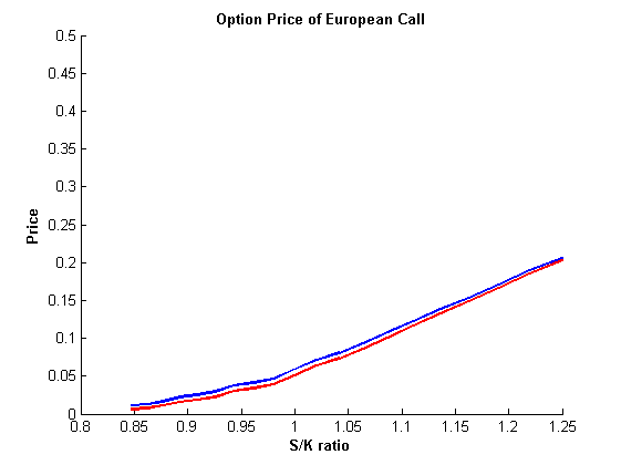
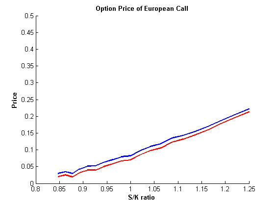
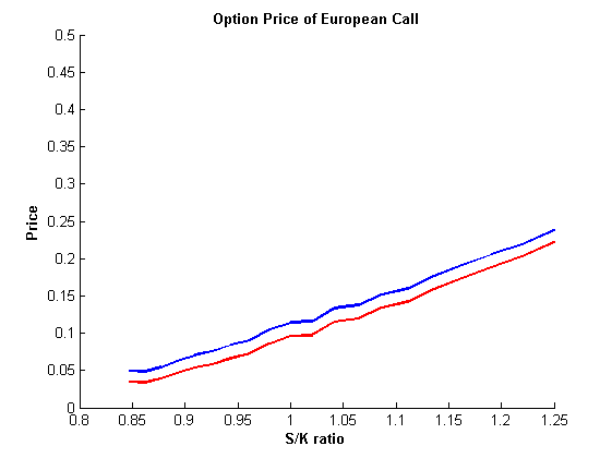
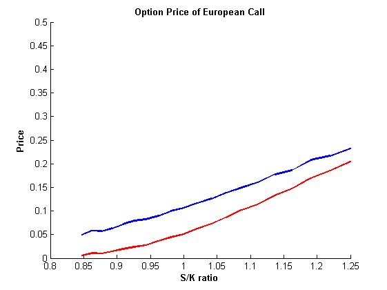
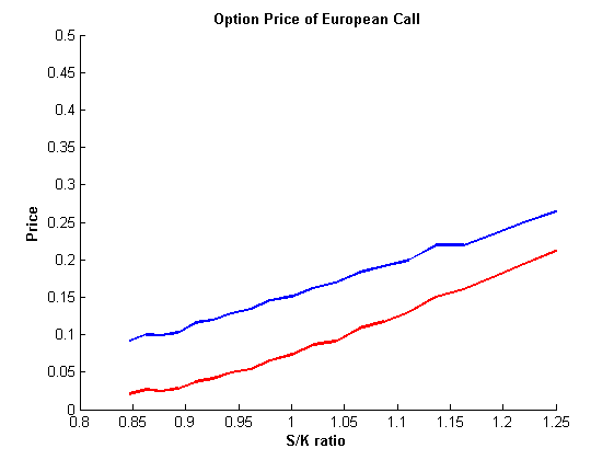
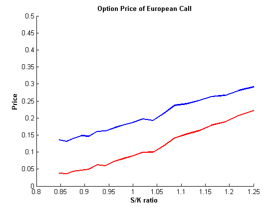
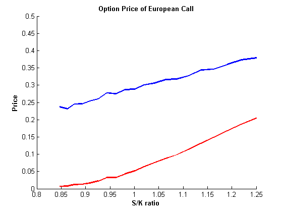
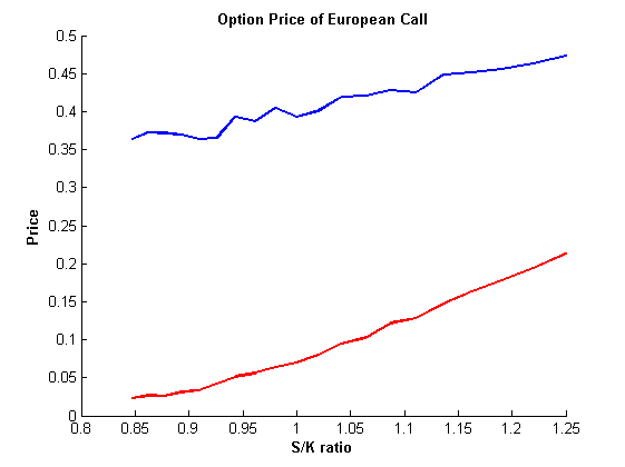
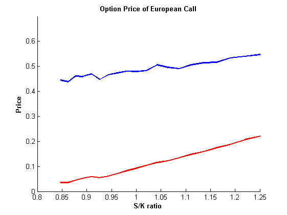
3) In section 4 we provide numerical simulations of European call foreign exchange option prices for different parameters: , where is the initial spot FX rate, is the strike FX rate for a maturity time .
Appendix contains the codes for Matlab functions used in numerical simulations of option prices.
2 Currency option pricing for Merton jump-diffusion processes
Let be a complete probability space with a probability measure P. Consider a continuous-time, finite-state Markov chain on with a state space , the set of unit vectors with a rate matrix 111In our numerical simulations we consider three-state Markov chain and calculate elements in using Forex market EURO/USD currency pair. The dynamics of the chain are given by:
| (1) |
where is a -valued martingale with respect to , the P-augmentation of the natural filtration , generated by the Markov chain . Consider a Markov-modulated Merton jump-diffusion which models the dynamics of the spot FX rate, given by the following stochastic differential equation (in the sequel SDE, see [20]):
| (2) |
Here is drift parameter; is a Brownian motion, is the volatility; is a Poisson Process with intensity , is the amplitude of the jumps, given the jump arrival time. The distribution of has a density . The parameters , , are modeled using the finite state Markov chain:
| (3) |
The solution of (2) is , (where is the spot FX rate at time ). Here is given by the formula:
| (4) |
Note, that for the most of well-known distributions (normal , exponential distribution of , etc) is not a Lvy process (see definition of Lvy process in [24], the condition L3), since for small , but probability of jumps with even 0 amplitude is a positive constant, depending on a type of distribution. We call the process (4) as Merton jump-diffusion process (see [23], section 2, formulas 2, 3)
There is more than one equivalent martingale measure for this market driven by a Markov-modulated jump-diffusion model. We shall define the regime-switching generalized Esscher transform to determine a specific equivalent martingale measure.
Using Ito’s formula we can derive a stochastic differential equation for the discounted spot FX rate. To define the discounted spot FX rate we need to introduce domestic and foreign riskless interest rates for bonds in the domestic and foreign currency.
The domestic and foreign interest rates , are defined using the Markov chain (see [20]):
The discounted spot FX rate is:
| (5) |
Using (5), the differentiation formula, see Elliott et al. (1982, [27]) and the stochastic differential equation for the spot FX rate (2) we find the stochastic differential equation for the discounted discounted spot FX rate:
| (6) |
To derive the main results consider the log spot FX rate
Using the differentiation formula:
| (7) |
| (8) |
Let denote the P-augmentation of the natural filtration , generated by . For each set . Let us also define two families of regime switching parameters
, : , , .
Define a random Esscher transform on using these families of parameters , (see [20], [25], [26] for details):
| (9) |
The explicit formula for the density of the Esscher transform is given in the following Theorem. A similar statement is proven for the log-normal distribution in [20]. The formula below can be obtained by another approach, considered by Elliott and Osakwe ([28]).
In addition,the random Esscher transform density (see (9), (10)) is an exponential martingale and admits the following SDE
| (11) |
Proof Theorem 2.1. The compound Poisson Process, driving jumps , and the Brownian motion are independent processes. As a result:
| (12) |
Let us calculate:
Write
Using the differentiation rule (see [27]) we obtain the following representation of :
| (13) |
where
is a martingale with respect to . Using this fact and (13) we obtain:
| (14) |
We have from the differentiation rule:
| (15) |
where is the volatility of a market. Substituting (14) and (15) into (12) we obtain:
| (17) |
If we present in the form (see (17)) and and apply differentiation rule we obtain SDE (11). It follows from (11) that is a martingale.
We shall derive the following condition for the discounted spot FX rate ((5)) to be martingale. These conditions will be used to calculate the risk-neutral Esscher transform parameters , and give to the measure Q. Then we shall use these values to find the no-arbitrage price of European call currency derivatives.
Theorem 2.2. Let the random Esscher transform be defined by (9). Then the martingale condition(for , see (5)) holds if and only if Markov modulated parameters () satisfy for all the condition:
| (18) |
where the random Esscher transform intensity of the Poisson Process and the main percentage jump size are respectively given by
| (19) |
| (20) |
as long as .
Proof of Theorem 2.2. The martingale condition for the discounted spot FX rate
| (21) |
To derive such a condition Bayes formula is used:
| (22) |
taking into account that is a martingale with respect to , so:
| (23) |
Using formula (5) for the solution of the SDE for the spot FX rate, we obtain an expression for the discounted spot FX rate in the following form:
Using expression for characteristic function of Brownian motion (see (15)) we obtain:
| (27) |
| (29) |
From (29) we get the martingale condition for the discounted spot FX rate:
| (30) |
Prove now, that under the Esscher transform the new Poisson process intensity and the mean jump size are given by (19), (20).
Note that is the jump part of Lvy process in the formula (4) for the solution of SDE for spot FX rate. We have:
| (31) |
where P is the initial probability measure, Q is a new risk-neutral measure. Substituting the density of the Esscher transform (10) into (31) we have:
| (32) |
Using (14) we obtain:
| (33) |
Putting (33) to (32) and taking into account characteristic function of Brownian motion (see (15)) we have:
| (34) |
Return to the initial measure P, but with different . We obtain:
| (35) |
Formula (19) for the new intensity of the Poisson process follows directly from (34),(35). The new density of jumps is defined from (34), (35) by the following formula:
| (36) |
Calculate now the new mean jump size given jump arrival with respect to the new measure Q:
| (37) |
So, we can rewrite martingale condition for the discounted spot FX rate in the form in (18), where are given by (19), (20) respectively.
Using (30) we have the following formulas for the families of the regime switching parameters satisfying the martingale condition (18):
| (38) |
| (39) |
where is any constant. Note again, that the choice for these parameters is not unique.
In the next section we shall apply these formulas (38), (39) to the exponential distribution of jumps.
We now proceed to the general formulas for European calls (see [20], [23]). For the European call currency options with a strike price and the time of expiration the price at time zero is given by:
| (40) |
Let denote the occupation time of in state over the period . We introduce several new quantities that will be used in future calculations:
| (41) |
where ;
| (42) |
| (43) |
| (44) |
| (45) |
where is the variance of the distribution of the jumps.
| (46) |
where is the number of jumps in the interval , is the number of states of the Markov chain .
From the pricing formula in Merton (1976, [23]) let us define (see [20])
| (47) |
where is the standard Black-Scholes price formula (see [21]) with initial spot FX rate , strike price , risk-free rate , volatility square and time to maturity.
Then, the European style call option pricing formula takes the form (see [20]):
| (48) |
where is the joint probability distribution density for the occupation time, which is determined by the following characteristic function (See [28]):
| (49) |
where is a vector of ones, is a vector of transform variables, .
3 Currency option pricing for exponential processes
Because of the restriction we can not consider a double-exponential distribution of jumps (see [29], [30]) in . Let us consider exponential distribution instead. It is defined by the following formula of density function:
| (50) |
The mean value of this distribution is:
| (51) |
The variance of this distribution is:
| (52) |
The exponential distribution like the double-exponential distribution has also memorylessness property.
Let us derive the martingale condition and formulas for the regime-switching Esscher transform parameters in case of jumps driven by the exponential distribution. Using the martingale condition for discounted spot FX rate (30) we obtain:
| (53) |
where we have such a restriction(and in the sequel): .
Using (19), (20) the random Esscher transform intensity of the Poisson Process and the main percentage jump size are respectively given by
| (54) |
| (55) |
Using (39) we have the following formula for the families of regime switching Esscher transform parameters satisfying martingale condition (53):
| (56) |
Let us simplify (56):
| (57) |
The formula for in this case is the same as in (38).
With respect to to such values of the regime switching Esscher transform parameters we have from (54), (55), (57):
| (58) |
| (59) |
From (59) we arrive at interesting conclusion: depends on time . So, now the distribution of jumps changes depending on time(it is not the case before for the log double-exponential distribution, where was actually a constant, see [20]). So, the compound Poisson Process depends not only on a number of jumps, but on moments of time when they arrive in this case. The same statement is true for the mean jump size in (55). But the pricing formulas (40)-(48) are applicable to this case as well.
In the numerical simulations, we assume that the hidden Markov chain has three states: up, down, side-way, and the corresponding rate matrix is calculated using real Forex data for the thirteen-year period: from January 3, 2000 to November 2013. To calculate all probabilities we use the Matlab script (see the Appendix).
4 Numerical simulations
In the following figures we shall provide numerical simulations for the case when amplitude of jumps is described by the exponential distribution. These plots show the dependence of a European-call option price on , where is the initial spot FX rate ( in our simulations)), is a strike FX rate for various maturity times 0.5, 1, 1.5 in years and various values of a parameter 2.5, 3.5, 5 in the exponential distribution. Blue line stands for the exponential distribution of jumps, red-line is for the dynamics without jumps. From these plots we can make a conclusion that it is important to incorporate a jump risk into the spot FX rate models (described by the Black-Scholes equation without jumps red line on a plot is below the blue line standing for the exponential distributions of jumps).
References
- [1] R. Jarrow and G. Oldfield , ‘‘Forward contracts and futures contracts. J. Financial Economics,’’ 9, 1981, pp. 373-382.
- [2] R. Merton , ‘‘The theory of rational option pricing,’’ Bell J. Econ. Manag. Sci., Spring, 4, 1973, pp. 141-183.
- [3] O. Grabbe , ‘‘The pricing of call and put options on foreign exchange,’’ J. Intern. Money and Finance, December, 2, 1983, pp. 239-253.
- [4] P. Adams and S. Wyatt , ‘‘Biases in option prices: Evidence from the foreign currency option market,’’ J. Banking and Finance, December, 11,1987, pp. 549-562.
- [5] K. Amin and R. Jarrow , ‘‘Pricing foreign currency options under stochastic interest rates,’’ J. Intern. Money and Finance, 10, 1991, pp. 310-329.
- [6] A. Melino and S. Turnbull, ‘‘The pricing of foreign-currency options,’’ Canadian J. Economics, 24, 1991, pp. 251-181.
- [7] J. Rumsey , ‘‘Pricing cross-currency options,’’ J. Futures markets, 11, 1991, pp. 89-93.
- [8] P. Mikkelsen , ‘‘Cross-currency LIBOR market model,’’ University of Aarhus, 2001.
- [9] E. Scholgl, ‘‘A multicurrency extension of the lognormal interest rate market models,’’ Finance and Stochastics, 6, 2002, pp. 173-196.
- [10] V. Piterbarg, ‘‘A multi-currency model with FX volatility skew,’’ Working paper, 2005.
- [11] M. Garman and S. Kohlhagern , ‘‘Foreign currency options values,’’ J. Intern. Money and Finance. 2, 1983, pp. 231-237.
- [12] A. Takahashi, K. Takehara and A. Yamazaki, ‘‘Pricing currency options with a market model of interest rates under jump-diffusion stochastic volatility processes of spot exchange rates,’’ CIRJE-F- 451, working paper, 2006.
- [13] F. Jamshidian , ‘‘LIBOR and swap market models and measures. Finance and Stochastics,’’ 1, pp. 293-330.
- [14] K. Miltersen, K. Sandmann and D. Sondermann, ‘‘Closed form solutions for term structure derivatives with long-normal interest rates,’’ J. Finance, 52, 1997, pp. 409-430.
- [15] C. Ahn , D. Cho and K. Park, ‘‘The pricing of foreign currency options under jump-diffusion processes,’’ J. Futures Markets, 27, 7, 2007, pp. 669-695.
- [16] S. Goutte and B. Zou, ‘‘Foreign exchange rates under Markov regime switching model,’’ CREA Discussion paper series, University of Luxemburg, 2011.
- [17] N. Zhou and R. S. Mamon, ‘‘An accessible implementation of interest rate models with regimeswitching,’’ Expert Systems with Applications, 39(5), 2012, pp. 4679-4689.DOI URL:10.1016/j.eswa.2011.09.053.
- [18] T.K. Siu , H. Yang and J. Lau, ‘‘Pricing currency options under two-factor Markov-modulated stochastic volatility model,’’ Insurance: Mathematics and Economics, 43, 2008, pp. 295-302.
- [19] A. Swishchuk , R. Eliott , ‘‘Pricing options. Hidden Markov Models in Finance,’’ Springer, 2007.
- [20] L. Bo , Y. Wang and X. Yang, ‘‘Markov-modulated jump-diffusion for currency option pricing,’’ Insurance: Mathematics and Economics, 46, 2010 , pp. 461-469.
- [21] T. Bjork, ‘‘Arbitrage Theory in Continuous Time,’’ 2nd ed. Oxford University Press, 1998.
- [22] F. Benth, J. Benth and S. Koekebakker, ‘‘Stochastic Modeling of Electricity and Related Markets,’’ World Scientific, 2008.
- [23] R.C.Merton, ‘‘Option pricing when underlying stock returns are discontinuous,’’ Journal of Finance and Economics 3, 1976, pp. 125-144.
- [24] A. Papapantoleon , ‘‘An introduction to Lvy processes with Applications to Mathematical Finance. Lecture notes,’’ 2000.
- [25] R.J. Elliott, L. Chan, T. K. Siu, ‘‘Option pricing and Esscher transform under regime switching,’’ Annals of Finance 1, 2005, pp. 423-432.
- [26] R.J. Elliott , T. K. Siu, L. Chan, J. W. Lau, ‘‘Pricing options under a generalized Markov-modulated jump-diffusion model,’’ Stochastic Analysis and Applications 25, 2007, pp. 821-843.
- [27] R. J. Elliott, ‘‘Stochastic Calculus and Applications,’’ Springer, 1982.
- [28] R. J. Elliott, Carlton-James U. Osakwe, ‘‘Option Pricing for Pure Jump Processes with Markov Switching Compensators,’’ Finance and Stochastics, Vol. 10, Issue 2, 2006, pp. 250-275.
- [29] S. G. Kou, ‘‘A jump-diffusion model for option pricing,’’ Management Science, 48(8), 2002, pp. 1086–1101.
- [30] Li-Hua Zhang, Wei-Guo Zhang, Wen-Jun Xu, Wei-Lin Xiao, ‘‘The double-exponential jump-diffusion model for pricing European options under fuzzy envirionments,’’ Economical Modelling, 29, 2012 , pp. 780-786.
Appendix
The Matlab function used to calculate probability matrix for the Markov chain modeling cross rates of currency pairs in the Forex market.
We assume that the Markov chain has only three states: "trend up", "trend down", "trend sideway". Such a choice of states is justified by numerous articles for the FX market (See www.mql5.com). In a file MaxDataFile open.CSV there are open prices of EURO/ESD currency pairs of Japanese candles over a 13 year period. This file was generated in the platform MT5 using MQL5 programming language.
function [ Probab_matrix ] =Probab_matrix_calc1(candles_back_up, candles_back_down,
delta_back_up, delta_back_down, candles_up,candles_down, delta_up, delta_down )
Probab_matrix=zeros(3,3);
m_open=csvread(’MaxDataFile_open.CSV’);
[size_open temp]=size(m_open);
m_before=zeros(1,size_open);
upper_border=size_open-max(candles_up, candles_down);
delta_up=delta_up/10000;
delta_down=delta_down/10000;
count_up=0;
count_down=0;
count_sideway=0;
beforeborder=max(candles_back_up, candles_back_down)+1;
for i=beforeborder:size_open
if (m_open(i)-m_open(i-candles_back_up)>=delta_up)
m_before(i)=1;
end
if (m_open(i-candles_back_down)-m_open(i)>=delta_down)
m_before(i)=-1;
end
end;
for i=1:upper_border
if(m_before(i)==1)
if(m_open(i+candles_up)-m_open(i)>=delta_up)
Probab_matrix(1,1)= Probab_matrix(1,1)+1;
else
if(m_open(i)-m_open(i+candles_down)>=delta_down)
Probab_matrix(1,2)= Probab_matrix(1,2)+1;
else
Probab_matrix(1,3)= Probab_matrix(1,3)+1;
end
end
end
if(m_before(i)==-1)
if(m_open(i+candles_up)-m_open(i)>=delta_up)
Probab_matrix(2,1)= Probab_matrix(2,1)+1;
else
if(m_open(i)-m_open(i+candles_down)>=delta_down)
Probab_matrix(2,2)= Probab_matrix(2,2)+1;
else
Probab_matrix(2,3)= Probab_matrix(2,3)+1;
end
end
end
if(m_before(i)==0)
if(m_open(i+candles_up)-m_open(i)>=delta_up)
Probab_matrix(3,1)= Probab_matrix(3,1)+1;
else
if(m_open(i)-m_open(i+candles_down)>=delta_down)
Probab_matrix(3,2)= Probab_matrix(3,2)+1;
else
Probab_matrix(3,3)= Probab_matrix(3,3)+1;
end
end
end
end
count_up=sum(Probab_matrix(1,:));
count_down=sum(Probab_matrix(2,:));
count_sideway=sum(Probab_matrix(3,:));
for j=1:3
Probab_matrix(1,j)= Probab_matrix(1,j)/count_up;
Probab_matrix(2,j)= Probab_matrix(2,j)/count_down;
Probab_matrix(3,j)= Probab_matrix(3,j)/count_sideway
end
end
For example run in Matlab:
[ Probab_matrix ] = Probab_matrix_calc1(30, 30, 10, 10, 30, 30, 10, 10);
Probability matrix is as follows: