Softness of Sn isotopes in relativistic semi-classical approximation

Abstract

Within the frame-work of relativistic Thomas-Fermi and relativistic extended Thomas-Fermi approximations, we calculate the giant monopole resonance (GMR) excitation energies for Sn and related nuclei. A large number of non-linear relativistic force parameters are used in this calculations. We find that a parameter set is capable to reproduce the experimental monopole energy of Sn isotopes, when its nuclear matter compressibility lies within $210-230$ MeV, however fails to reproduce the GMR energy of other related nuclei. That means, simultaneously a parameter set can not reproduce the GMR values of Sn and other nuclei.

I Introduction

Incompressibility of nuclear matter, also knows as compressional modulus has a special interest in pure nuclear and astro-nuclear physics, because of its fundamental role in guiding the equation of state (EOS) for nuclear matter. Compressional modulus $K_{\infty}$ can not be measured by any experimental technique directly, rather it depends indirectly on the experimental measurement of isoscalar giant monopole resonance (ISGMR) for its conformation blaizot . This fact enriches the demand of correct measurement of excitation energy of ISGMR. The relativistic parameter with random phase approaches (RPA) constraint the range of the compressibility modulus $270\pm{10}$ MeV lala97 ; Vrete02 for nuclear matter. Similarly, the non-relativistic formalism with Hartree-Fock (HF) plus RPA allows the acceptable range of compressibility modulus $210-220$ MeV, which is less than relativistic one. It is believed that the part of this discrepancy in the acceptable range of compressional modulus comes from the diverse behavior of the density dependence of symmetry energy in relativistic and non-relativistic formalism horow02 ; horowr01 . Now, both the relativistic and non-relativistic formalisms come with a general agreement on the value of nuclear compressibility i.e., $240\pm{10}$ MeV colo04 ; todd05 ; Agrawal05 . But the new experiment on $Sn$ isotopic series i.e., ${}^{112}Sn-^{124}Sn$ rises the question ”why Tin is so fluffy ?”ugarg ; tli07 ; ugarg07 . This question again finger towards the correct theoretical investigation of compressibility modulus.

Thus, it is worthy to investigate the compressibility modulus in various theoretical formalisms. Most of the relativistic and non-relativistic theoretical models reproduce the strength distribution very well for medium and heavy nuclei, like ${}^{90}Zr$ and ${}^{208}{Pb}$, respectively. But at the same time it overestimate the excitation energy of $Sn$ around 1 MeV. This low value of excitation energy demands lower value nuclear matter compressibility. This gives a new challenge to both the theoretical and experimental nuclear physicsts. Till date, lots of effort have been devoted to solve this problem like inclusion of pairing effect citav91 ; gang12 ; jun08 ; khan09 , mutually enhancement effect (MEM) etc. khana09 . But the pairing effect reduces the theoretical excitation energy only by 150 KeV in $Sn$ isotopic series, which may not be sufficient to overcome the puzzle. Similarly, new experimental data are not in favor of MEM effectdpatel13 . Measurement on excitation energy of ${}^{204,206,208}Pb$ shows that the MEM effect should rule out in manifestation of stiffness of the $Sn$ isotopic series.

Here, in the present work, we use the relativistic Thomas-Fermi (RTF) and relativistic extended Thomas-Fermi (RETF) acentel93 ; acentel92 ; speich93 ; centel98 ; centell93 with scaling and constraint approaches in the frame-work of non-linear $\sigma-\omega$ model bo77 . The RETF is the $\hbar^{2}$ correction to the RTF, where variation of density taken care properly mostly in the surface of the nucleus cetelles90 . The RETF formalism is more towards the quantal Hartee approximation. It is also verified that the semiclassical approximation like Thomas-Fermi method is very useful in calculation of collective property of nucleus, like giant monopole resonance (GMR). In particular, for heavier mass nuclei, it gives almost similar results with the complicated quantal calculation. This is because of quantal correction are averaged out in heavier mass nuclei and results are inclined toward semiclassical one. So it is very much instructive to calculate excitation energy of various nucleus by this method and compared with experimental results. Since, last one decade, the softness of Sn isotopes remain a headache for both theorists and experimentalists, it is worthy to discuss the softness of Tin isotopes in semiclassical approximations like RETF and RTF.

Here, we calculate the excitation energy of Sn isotopes from ¹¹²Sn to ¹²⁴Sn using the semi-classical RTF and RETF model. The different momentum ratio like $(m_{3}/m_{1})^{1/2}$ and $(m_{1}/m_{-1})^{1/2}$ are compared with the scaling and constraint calculations. The theoretical results are computed in various parameter sets such as NL-SH, NL1, NL2, Nl3 and FSUG. We analyzed the predictive power of these parameter sets and discussed various aspects of the compressibility modulus.

This paper is organized as follow: In Section II we have summarized the theoretical formalisms, which are useful for the present analysis. In section III, we have given the discussions of our results. Here, we have elaborated the giant monopole resonance obtained by various parameter sets and their connectivity with compressibility modulus. The last section is devoted to a summary and concluding remarks.

II Theoretical framework

The principle of scale invariance is used to obtain the virial theorem for the relativistic mean field serot86 theory by working in the relativistic Thomas–Fermi (RTF) and relativistic extended Thomas-Fermi (RETF) approximations patra01 ; acentel93 ; acentel92 ; spei98 ; mario98 ; mario93a . Although, the scaling and constrained calculations are not new, the present technique is developed first time by Patra et al patra01 ; mario10 , which is different from other scaling formalisms.

The detail formalisms of the scaling method are given in Refs. patra01 ; patra02 . For completeness, we have outlined briefly some of the essential expressions, which are needed for the present purpose. We have worked with the non-linear Lagrangian of Boguta and Bodmer bo77 to include the many-body correlation arises from the non-linear terms of the $\sigma-$meson self-interaction schiff51 ; fujita57 ; steven01 for nuclear many-body system. The nuclear matter compressibility modulus $K_{\infty}$ also reduces dramatically by the introduction of these terms, which motivates to work with this non-liner Lagrangian. The relativistic mean field Hamiltonian for a nucleon-meson interacting system is written by serot86 ; patra01 :

$${\cal H} = \sum_{i}\varphi_{i}^{\dagger}\bigg{[}-i\vec{\alpha}\cdot\vec{\nabla}+\beta m^{*}+g_{v}V+\frac{1}{2}g_{\rho}R\tau_{3}$$ (1)

$$+ \frac{1}{2}e{\cal A}(1+\tau_{3})\bigg{]}\varphi_{i}+\frac{1}{2}\left[(\vec{\nabla}\phi)^{2}+m_{s}^{2}\phi^{2}\right]+\frac{1}{3}b\phi^{3}$$

$$+ \frac{1}{4}c\phi^{4}-\frac{1}{2}\left[(\vec{\nabla}V)^{2}+m_{v}^{2}V^{2}\right]$$

$$- \frac{1}{2}\left[(\vec{\nabla}R)^{2}+m_{\rho}^{2}R^{2}\right]-\frac{1}{2}\left(\vec{\nabla}{\cal A}\right)^{2}-\frac{\zeta_{0}}{24}g_{v}^{4}{V}^{4}$$

$$- {\Lambda_{V}}{g_{v}^{2}}{g_{\rho}}^{2}{R^{2}}{V^{2}}$$ (2)

Here $m$, $m_{s}$, $m_{v}$ and $m_{\rho}$ are the masses for the nucleon (with $m^{*}=m-g_{s}\phi$ being the effective mass of the nucleon), ${\sigma}-$, $\omega-$ and ${\rho}-$mesons, respectively and ${\varphi}$ is the Dirac spinor. The field for the ${\sigma}$-meson is denoted by ${\phi}$, for ${\omega}$-meson by $V$, for ${\rho}$-meson by $R$ ($\tau_{3}$ as the $3^{rd}$ component of the isospin) and for photon by $A$. $g_{s}$, $g_{v}$, $g_{\rho}$ and $e^{2}/4{\pi}$=1/137 are the coupling constants for the ${\sigma}$, ${\omega}$, ${\rho}$-mesons and photon respectively. $b$ and $c$ are the non-linear coupling constants for ${\sigma}$ mesons. By using the classical variational principle we obtain the field equations for the nucleon and mesons. In semi-classical approximation, we can write the above Hamiltonian in term of density as:

$${\cal H} = {\cal E}+g_{v}V{\rho}+g_{\rho}R{\rho}_{3}+e{\cal A}{\rho}_{p}+{\cal H}_{f},$$ (3)

where

$${\cal E} = \sum_{i}\varphi_{i}^{\dagger}\bigg{[}-i\vec{\alpha}\cdot\vec{\nabla}+\beta m^{*}\bigg{]}\varphi_{i},$$ (4)

$${\rho}_{s} = \sum_{i}\varphi_{i}^{\dagger}{\varphi},$$ (5)

$${\rho} = \sum_{i}{\bar{\varphi}_{i}}{\varphi},$$ (6)

$${\rho_{3}} = \frac{1}{2}\sum_{i}{\varphi}_{i}^{\dagger}{\tau_{3}}{\varphi}_{i},$$ (7)

and ${\cal H}_{f}$ is the free part of the Hamiltonian. The total density $\rho$ is the sum of proton $\rho_{p}$ and neutron $\rho_{n}$ densities. The semi-classical ground-state meson fields are obtained by solving the Euler–Lagrange equations $\delta{\cal H}/\delta\rho_{q}=\mu_{q}$ ($q=n,p$).

$$(\Delta-m_{s}^{2})\phi=-g_{s}\rho_{s}+b\phi^{2}+c\phi^{3},\\$$ (8)

$$(\Delta-m_{v}^{2})V = -g_{v}\rho+2{\Lambda_{V}}{R^{2}}V$$ (9)

$$+ \frac{\zeta_{0}}{6}{g_{v}^{4}}V^{3}$$ (10)

$$(\Delta-m_{\rho}^{2})R=-g_{\rho}\rho_{3}+2{\Lambda_{V}}R{V^{2}},$$ (11)

$$\Delta{\cal A}=-e\rho_{p}.$$ (12)

The above field equations are solved self-consistently in an iterative method.

$${\cal H}={\cal E}+\frac{1}{2}g_{s}\phi\rho^{eff}_{s}+\frac{1}{3}b\phi^{3}+\frac{1}{4}c\phi^{4}+\frac{1}{2}g_{v}V\rho+\frac{1}{2}g_{\rho}R\rho_{3}+\frac{1}{2}e{\cal A}\rho_{p}\\ -2{\Lambda_{V}}{R^{2}}{V^{2}}-\frac{\zeta_{0}}{12}{g_{v}}^{4}{V^{4}},$$ (13)

with

$${\rho}_{s}^{eff} = g_{s}{\rho}_{s}-b{\phi}^{2}-c{\phi}^{3}.$$ (14)

In order to study the monopole vibration of the nucleus we have scaled the baryon density patra01 . The normalized form of the baryon density is given by

$${\rho}_{\lambda}\left(\bf r\right) = {\lambda}^{3}{\rho}\left(\lambda r\right),$$ (15)

${\lambda}$ is the collective co-ordinate associated with the monopole vibration. As Fermi momentum and density are inter-related, the scaled Fermi momentum is given by

$$K_{F}q{\lambda} = \left[3{\pi}^{2}{\rho}_{q}\lambda\left(\bf r\right)\right]^{\frac{1}{3}}.$$ (16)

Similarly $\phi$, $V$, $R$ and Coulomb fields are scaled due to self-consistence eqs. (7-10). But the $\phi$ field can not be scaled simply like the density and momentum, because the source term of $\phi$ field contains the $\phi$ field itself. In semi-classical formalism, the energy and density are scaled like

$${\cal E_{\lambda}}(\bf r) = {\lambda}^{4}{\tilde{\cal E}}(\lambda\bf r)$$ (17)

$$= \lambda^{4}[\tilde{\cal E}_{0}(\lambda\bf r)+\tilde{\cal E}_{2}(\lambda\bf r)],$$

$$\rho_{{s\lambda}}(\bf r)={\lambda^{3}}{\tilde{\rho}}_{s}{(\lambda{\bf r})}.$$ (18)

The symbol $\sim$ shows an implicit dependence of $\tilde{m}^{*}$. With all these scaled variables, we can write the Hamiltonian as:

$${\cal{H}}_{\lambda} = {\lambda^{3}}{\lambda}{\tilde{\cal{E}}}+\frac{1}{2}{g_{s}}\phi_{\lambda}{{\tilde{\rho}}_{s}^{eff}}+\frac{1}{3}\frac{b}{\lambda^{3}}\phi_{\lambda}^{3}+\frac{1}{4}\frac{c}{\lambda^{3}}{\phi_{\lambda}}^{4}$$ (19)

$$+ \frac{1}{2}{g_{v}}V_{\lambda}{\rho}+\frac{1}{2}g_{\rho}R_{\lambda}{\rho_{3}}+\frac{1}{2}e{A}_{\lambda}{\rho}_{p}$$

$$- 2\Lambda_{V}{R_{\lambda}}^{2}{V_{\lambda}}^{2}-\frac{\zeta_{0}}{12}{g_{v}^{4}}{V_{\lambda}}^{4}$$ (20)

Here we are interested to calculate the monopole excitation energy which is defined as ${E}^{s}={\sqrt{\frac{C_{m}}{B_{m}}}}$ with ${C_{m}}$ is the restoring force and $B_{m}$ is the mass parameter. In our calculations, $C_{m}$ is obtained from the double derivative of the scaled energy with respect to the scaled co-ordinate $\lambda$ at ${\lambda}=1$ and is defined as patra01 :

$${C}_{m} = \int{dr}\bigg{[}-m\frac{\partial{\tilde{\rho_{s}}}}{\partial{\lambda}}+3\bigg{(}{m_{s}}^{2}{\phi}^{2}+\frac{1}{3}b{\phi}^{3}$$ (21)

$$- {m_{v}}^{2}{V^{2}}-{m_{\rho}}^{2}R^{2}\bigg{)}-(2{m_{s}}^{2}{\phi}+b{\phi}^{2})\frac{\partial{\phi_{\lambda}}}{\partial{\lambda}}$$

$$+ 2{m_{v}}^{2}V\frac{\partial{V_{\lambda}}}{\partial{\lambda}}+2{m_{\rho}}^{2}R\frac{\partial R_{\lambda}}{\partial\lambda}\bigg{]}_{\lambda=1},$$

and the mass parameter $B_{m}$ of the monopole vibration can be expressed as the double derivative of the scaled energy with the collective velocity $\dot{\lambda}$ as

$$B_{m}=\int{dr}{U(\bf r)}^{2}{\cal{H}},$$ (22)

where $U(\bf r)$ is the displacement field, which can be determined from the relation between collective velocity $\dot{\lambda}$ and velocity of the moving frame,

$$U(\bf r)=\frac{1}{\rho(\bf r){\bf r}^{2}}\int{dr^{\prime}}{\rho}_{T}(r^{\prime}){r^{\prime}}^{2},$$ (23)

with ${\rho}_{T}$ is the transition density defined as

$${{\rho}_{T}(\bf r)}=\frac{\partial{\rho_{\lambda}(\bf r)}}{\partial{\lambda}}\bigg{|}_{\lambda=1}=3{\rho}(\bf r)+r\frac{\partial{\rho(\bf r)}}{\partial r},$$ (24)

taking $U(\bf r)=r$. Then the mass parameter can be written as $B_{m}=\int{dr}{r}^{2}{\cal H}$. In non-relativistic limit, ${B_{m}}^{nr}=\int{dr}{r^{2}}m{\rho}$ and the scaled energy ${E_{m}}^{s}$ is $\sqrt{\frac{m_{3}}{m_{1}}}$. The expressions for ${m_{3}}$ and ${m_{1}}$ can be found in bohigas79 . Along with the scaling calculation, the monopole vibration can also be studied with constrained approach bohigas79 ; maru89 ; boer91 ; stoi94 ; stoi94a . In this method, one has to solve the constrained functional equation:

$$\int{dr}\left[{\cal H}-{\eta}{r}^{2}{\rho}\right]=E(\eta)-\eta\int{dr}{r}^{2}\rho.$$ (25)

Here the constrained is ${\langle{R^{2}}\rangle}_{0}={\langle{r^{2}}\rangle}_{m}$. The constrained energy $E(\eta)$ can be expanded in a harmonic approximation as

$$E(\eta) = E(0)+\frac{\partial E(\eta)}{\partial\eta}\big{|}_{\eta=0}+\frac{\partial^{2}{E(\eta)}}{\partial{\eta}^{2}}|_{\eta=0}.$$ (26)

The second order derivative in the expansion is related with the constrained compressibility modulus for finite nucleus $K_{A}^{c}$ as

$${K_{A}}^{c}=\frac{1}{A}{R_{0}}^{2}\frac{\partial^{2}{E\eta}}{\partial{R_{\eta}}},$$ (27)

and the constrained energy ${{E_{m}}^{c}}$ as

$${{E_{m}}^{c}}={\sqrt{\frac{A{K_{A}^{c}}}{B_{m}^{c}}}}.$$ (28)

In the non-relativistic approach, the constrained energy is related by the sum rule weighted ${{E_{m}}^{c}}={\sqrt{\frac{m_{1}}{m_{-1}}}}$. Now the scaling and constrained excitation energies of the monopole vibration in terms of the non-relativistic sum rules will help us to calculate $\sigma$, i.e. the resonance width bohigas79 ; centelle05 ,

$${\sigma} = \sqrt{\left({E_{m}}^{s}\right)^{2}-\left({E_{m}}^{c}\right)^{2}}=\sqrt{({\frac{m_{3}}{m_{1}}})^{2}-{(\frac{m_{1}}{m_{-1}}})^{2}}.$$ (29)

III Results and Discussions

It is interesting to apply the model to calculate the excitation energy of Sn isotopic series and compared with experimental results. Thus, we calculate the GMR energy using both the scaling and constraint methods in the frame-work of relativistic extended Thomas-Fermi approximation using various parameter sets for Z= 48 and 50 and compared with the excitation energy with momentum ratio $m_{3}/m_{1}$ and $m_{1}/m_{-1}$ obtained from multipule decomposition analysis (MDA). The basic reason to take a number of parameter sets is that the infinite nuclear matter compressibility of these forces cover a wide range of values. For example, NL-SH has compressibility 399 MeV, while that of NL1 is 210 MeV. From MDA analysis we get different momentum ratio, such as $m_{3}/m_{1}$, $m_{0}/m_{1}$ and $m_{1}/m_{-1}$. These ratios are connected to scaling, centroid and constraint energies, respectively. That is why we compared our theoretical scaling result with $({m_{3}/m_{1}})^{1/2}$ and $({m_{1}/m_{-1}})^{1/2}$ with the constrained calculations.

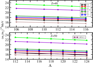
Figure 1: Giant monopole excitation energy obtained by scaling method with various parameter sets are compared with experimental ugarg ; tli07 ; ugarg07 $({m_{3}/m_{1}})^{1/2}$ for Cd and Sn isotopes.

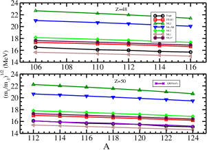
Figure 2: Same as Fig. 1, but for $({m_{1}/m_{-1}})^{1/2}$.

In Figures 1 and 2 we have shown the $(m_{3}/m_{1})^{1/2}$ and $(m_{1}/m_{-1})^{1/2}$ ratio for isotopic chains of Cd and Sn. The results are also compared with experimental data obtained from (RCNP) ugarg ; tli07 ; ugarg07 . From the figures, it is cleared that the experimental value lies between the results obtained from FUSG (FSUGold) and NL1 force parameters. It is to be noted that, throughout the calculations, we have used only the non-linner parameter sets for their excellent prediction of nuclear observables with the experimental data. If one compares the experimental and theoretical results for ²⁰⁸Pb, the FSUG set gives better results amongst all. For example, the experimental and theoretical data are 14.17$\pm$0.1 and 14.04 MeV, respectively. These values are well matched with each other. From this, one could conclude that the infinite nuclear matter compressibility lies nearer to that of FSUG (230.28 MeV) parameter. But experimental result on ISGM in RCNP shows that the predictive power of FUSG is not good enough for the excitation energy of Sn isotopes. This observation is not only confined to RCNP formalism, but also persists in the more sophisticated RPA approach. In Table I, we have given the results for QRPA(T6), RETF(FSUG) and RETF(NL1). The experimental data are also given to compare all these theoretical results.

Table 1: Momentum ratio for Sn isotopes using RETF approximation with FSUGold and NL1 sets are compared with QRPA(T6) predictions tsel09 .

Nucleus	$({m_{3}/m_{1}})^{1/2}$(MeV)				$({m_{1}/m_{-1}})^{1/2}$(MeV)
	QRPA(T6)	RETF(FSUG)	RETF(NL1)	Expt.	QRPA(T6)	RETF(FSU)	RETF(NL1)	Expt.
112Sn	17.3	17.42	15.86	16.7	17.0	17.2	15.39	16.1
114Sn	17.2	17.32	15.75	16.5	16.9	16.9	15.28	15.9
116Sn	17.1	17.19	15.63	16.3	16.8	16.77	15.15	15.7
118Sn	17.0	17.07	15.51	16.3	16.6	16.63	15.03	15.6
120Sn	16.9	16.94	15.38	16.2	16.5	16.44	14.89	15.5
122Sn	16.8	16.81	15.24	15.9	16.4	16.34	14.75	15.2
124Sn	16.7	16.67	15.1	15.8	16.2	16.19	14.6	15.1

The infinite nuclear matter compressibility $K_{\infty}$ with T6 parameter set is 236 MeV and that of FSUG is 230.28 MeV. The difference in $K_{\infty}$ between these two sets is only 6 MeV. The similarity in compressibility (small difference in $K_{\infty}$) may be a reason for their prediction in equal value of GMR. The table shows that, there is only 0.1 MeV difference in QRPA(T5) and RETF(FSU) results in the GMR values for ¹¹²Sn$-$¹¹⁶Sn isotopes, but the results are exactly matched for the ¹¹⁸Sn$-$¹²⁴Sn. This implies that for relatively higher mass nuclei, both the QRPA(T6) and RETF(FSUG) results are almost similar. If some one consider the experimental value of Sn isotopic series, then QRPA(T5) gives better result. For example, experimental value of $(m_{3}/m_{1})^{1/2}$ for ¹¹²Sn is 16.7$\pm$ 0.2 MeV and that for QRPA(T5) is 16.6 MeV. These two values matches well with each other. The infinite nuclear matter compressibility of T5 set is 202 MeV. It is shown by V. Tselyaev et al. tsel09 that the T5 parameter set with such compressibility, better explains the excitation energy of Sn isotopes, but fails to predict the excitation energy of ²⁰⁸Pb. It over estimates the data for ²⁰⁸Pb. The experimental data of ISGMR energies for ⁹⁰Zr and ¹¹⁴Sn lies in between the calculated values of T5 and T6 forces. In summary, we can say that the RPA analysis predicts the symmetric nuclear matter compressibility within $202-236$ MeV and our semi-classical calculation gives it in the range $210-230$ MeV. These two predictions almost agree with each other in the acceptable limit.

Table 2: Momentum ratio ${\sqrt{{m_{1}/m_{-1}}}}$ for Pb isotopes within RETF is compared with pairing+ MEM results and experimental data dpatel13 .

Nuclear Mass	${m_{1}/m_{-1}}^{1/2}$ (MeV)			$\Gamma$
	pairing+MEM	Our work	Expt.	our work	Expt.
${}^{204}Pb$	13.4	13.6	13.7$\pm$0.1	2.02	3.3$\pm$0.2
${}^{206}Pb$	13.4	13.51	13.6$\pm$0.1	2.03	2.8$\pm$0.2
${}^{208}Pb$	13.4	13.44	13.5$\pm$0.1	2.03	3.3$\pm$0.2

In Table II, we have displayed the data obtained from a recent experiment dpatel13 and compared our results. Column two of the table is also devoted to the result obtained from pairing plus MEM effect khan09 . The data show clearly that our result (extended Thomas-Fermi) has a priority over the pairing + MEM prediction. For example, the difference between the pairing+MEM results and experimental observation is 0.3 MeV for ²⁰⁴Pb isotopes, which is away from the experimental error, while it is only 0.1 MeV (within the error bar) in the RETF and data. This trend also followed by ²⁰⁶Pb and ²⁰⁸Pb nuclei. In our model, we have not included any pairing externally. But still our results are good enough in comparision with MEM+pairing. This implies two things: (i) pairing may not be impotant in calculation of excitation energy or (ii) pairing effect is automatically included in Thomas-Fermi calculations.

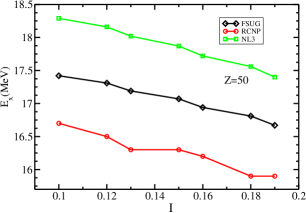
Figure 3: The variation of giant monopole excitation energy $E_{X}$ with proton-neutron asymmetry I=(N-Z)/(N+Z) for Sn isotopes.

To our understanding, the second option seems to be more appropiate, because lots of work show that pairing must be included for the calculation of excitation energy of open shell nuclei. Fig. 3 shows the variation of excitation energy with proton-neutron asymetry in Sn isotopes. Here, we want to know, how the excitation energy varies with asymetry or more specifically, ”is the variation of experimental excitation energy with asymetry same that of theoritical one ?”. The graph shows that the variation with both NL1 and FSUG are following similar partten as experimental one with a different mangnitued as shown in the figure.

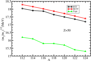
Figure 4: The scaling monopole excitation energy within RETF and RTF formalisms compared with the experimental momentum ratio ${m_{3}/m_{1}}^{1/2}$ dpatel13 .

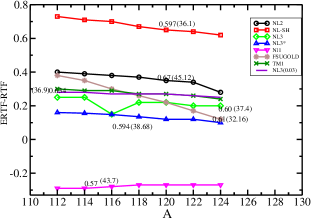
Figure 5: The variation of the difference of giant monopole excitation energy obtained from RETF and RTF (RETF-RTF) formalisms with various parameter sets for Sn isotopic chain.

In Figure 4, we have compared the results obtained from RETF and RTF with the experimental data for Sn isotopes. The celebraty NL3 parameter set is used in the calculations. The graph shows that there is only a small difference ($\sim 0.2$ MeV) in RETF and RTF results. Interestingly, the RETF correction is additive to the RTF result instead of softening the excitation energy of Sn isotopes. Then the natural question arises: is it the brhavior for all the parameter sets in RETF approximation ?. To attend the question, we plotted Fig. 5, where we have shown the difference of ${\sqrt{m_{3}/m_{1}}}$ obtained with RETF and RTF results (RETF-RTF) for various parameter sets. For all sets, except NL1, we find RETF-RTF as positive. Thus, it is a challenging task to antangle the term which is the responsible factor to determine the sign of RETF-RTF. Surprisingly, for most of the parameter sets, RTF is more towards experimental data. Inspite of this, one cannot says anything about the qualitative behavior of RETF. Because, the variation of the density at the surface taken care properly by RETF formalism, which is essential. One more interesting observation is that, when one investigate the variation of RETF-RTF in the isotopic chain of Sn, it remains almost constant for all the parameter sets, except FSUG. In this context, FSUG behaves differently.

Variation of RETF-RTF with neutron-proton asymmetry for FSUG set shows that, there may be some correlation of RETF with the symmetry energy. This is clearly absent in all other parameter sets. Now it is essential to know, in which respect the FSUG parameter set is different from other. The one-to-one interaction terms for NL3, NL2, NL1 and NL-SH all have similar couplings. However, the FSUG is different from the above parameters in two aspect, i.e., two new coupling constants are added. One corresponds to the self-interaction of $\omega$ and other one corresponds to the isoscalar-isovector meson coupling. It is known that self-interaction of $\omega$ is responsible for softening the EOS gmuca ; toki94 ; bodmer91 and the isoscalar-isovector coupling takes care of the softening for symmetry energy of symmetric nuclear matterhorow02 . The unique behavior shown by the FSUG parametrization may be due to the following three reasons:

1. introduction of isoscalar-isovector meson coupling $\Lambda_{V}$.

2. introduction of self-coupling of $\omega-$meson.

3. Or simultaneous introduction of both these two terms with refitting of parameter set with new constraint.

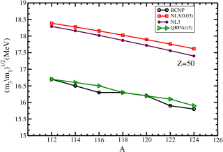
Figure 6: The momentum ratio ${\sqrt{{m_{3}/m_{1}}}}$ for Sn isotopes obtained with NL3+$\Lambda_{V}$ is compared with NL3, QRPA(T5) and experimental data.

In order to discuss the first possibility, we plotted NL3+$\Lambda_{V}$(0.03) in Figure 6. The graph shows that there is no difference between NL3 and NL3+$\Lambda$, except the later set predicts a more possitive RETF-RTF. It is well known that, the addition of $\Lambda_{V}$ coupling, i.e., NL3+$\Lambda_{V}$(0.03) gives of a softer symmetry energy patra9 . This implies that, models with softer energy have greater difference in RETF and RTF. At a particular proton-neutron asymmetry, RETF-RTF has a larger value for a model with softer symmetry energy. This observation is not conclusive, because all the parameter sets do not follow this type of behavior. Quantitatively, the change of RETF-RTF in the Sn isotopic series is about $70\%$, while this is only $20-30\%$ in NL3 and other parameter set.

In Table III, we have listed the $\rho-$meson contribution to the total energy. From the analysis of our results, we find that only $\rho-$contribution to the total binding energy change much more than other quantity, when one goes from RTF to RETF. But this change is more prominent in FSUG parameter set than other sets like NL1, NL2, NL3 and NL-SH. Simple assumption says that, may be the absent of $\Lambda_{V}$ term in other parameter is the reason behind this. But we have checked for the parameter NL3+$\Lambda_{V}$, which does not follow. This also shows similar behavior like other sets. In Table IV, we have given the results for FSUG, NL3+$\Lambda_{V}$ and NL1. The data show clearly that, there is a huge difference of monopole excitation energy in RETF and RTF with FSUG parameter set. For example, the $\rho-$meson contribution to the GMR in RETF for ¹¹²Sn is 21.85 MeV, while in RTF it is only 0.00467 MeV.

Table 3: Contribution of the $\rho-$meson to the total binding energy in the RTF and RETF approximations with FSUGold and NL1 parameter set.

Mass	FSUG				NL3(0.03)		NL1
	RETF	RTF	RETF$\Lambda_{V}$	RTF$\Lambda_{V}$	RETF	RTF	RETF	RTF
112	21.85	-6.66	-0.00130	0.00467	20.60	20.12	17.91	16.73
114	28.72	-8.64	-0.00202	0.00664	27.11	26.48	23.51	22.00
116	36.42	-10.83	-0.00248	0.00829	34.40	33.62	29.73	27.90
118	44.87	-13.23	-0.00298	0.01013	42.42	41.499	36.52	34.37
120	54.04	-15.82	-0.00353	0.01213	51.13	50.05	43.84	41.37
122	63.88	-18.58	-0.00411	0.01429	60.48	59.24	51.63	48.85
124	74.33	-21.49	-0.00473	0.01660	70.43	69.03	59.84	56.76

However, this difference is nominal in NL3+$\Lambda_{V}$ parameter set, i.e., it is only 0.48 MeV. Similarly, this value is 1.18 MeV in NL1 set. The contribution of $\rho-$meson to total energy comes from two terms: (i) one from $\Lambda_{V}{R^{2}}{V^{2}}$ and other (ii) from $\rho^{2}$. We have explicitly shown that contribution comes from $\Lambda_{V}{R^{2}}{V^{2}}$ makes a huge difference between the GMR obtained from RETF and RTF formalisms. This type of contribution does not appear from NL3+$\Lambda_{V}$. For example, in ¹¹²Sn the contribution of $\Lambda_{V}{R^{2}}{V^{2}}$ with RETF formalism is -6.0878 MeV, while with RTF formalism is -5.055 MeV.

The above discussion gives us a significant signiture that the contribution of $\Lambda_{V}$ may be responsible for this anomalous behavior. But an immediate question arises , why NL3+$\Lambda_{V}$ parameter set does not show such type of effects, inspite of having $\Lambda_{V}{R^{2}}{V^{2}}$ term. This may be due to the procedure in which $\Lambda_{V}{R^{2}}{V^{2}}$ term is added in two parameters. In NL3+$\Lambda_{V}$(0.03), the $\Lambda_{V}{R^{2}}{V^{2}}$ term is not added independently. The $\Lambda_{V}$ and $g_{\rho}$ are interdependent to each other to fix the binding energy BE and difference in neutron and proton rms radii $R_{n}$-$R_{p}$. But in FSUGold, $\Lambda_{V}$ coupling constant is added independenly to reproduce the nuclear observables.

Table 4: ${}^{S}K_{A}$ and ${}^{C}K_{A}$ are compressibility of finite nuclei obtained from scaling and costraint methods, respectively are compared with the values obtained from the equation of state (EOS).

Nuclear Mass	NL3			FSUGOLD
	${}^{S}K$	${}^{C}k$	${}^{EOS}K$	${}^{S}K$	${}^{C}K$	${}^{EOS}K$
${}^{208}Pb$	164.11	149.96	145	147.37	134.57	138.42
${}^{116}Sn$	164.64	155.39	131.57	147.11	139.71	127.64
40P	136.70	110.43	105	123.40	100.36	102.53
40Ca	145.32	134.47	105	130.93	123.15	102.53

In Table IV, we have listed the compressibility of some of the selected nuclei in scaling ${}^{S}K_{A}$ and constraint ${}^{C}K_{A}$ icalculations. This results are compared with the computed values obtained from EOS model. To evaluate the compressibility from EOS, we have followed the procedure discussed in centelles09 ; shailesh13 . M. Centelles et al centelles09 , parameterised the density for finite nucleus as $\rho_{A}=\rho_{0}-\rho_{0}/(1+c*{A^{1/3}})$ and obtained the asymmetry coefficient $a_{sym}$ of the nucleus with mass A from the EOS at this particular density. Here also, we have used the same parametric from of the density and obtained the compressibility of finite nucleus from the EOS. For example, $\rho_{A}=0.099$ for $A=208$ in FSUG parameter set. We have calculated the compressibility from the EOS at this particular density, which comes around 145 MeV. We have also calculated the compressibility independently in Thomas-Fermi and extended Thomas-Fermi using scaling and constraint calculations, which are 161 MeV and 146.1 MeV, respectively.

IV Summary and Conclusion

In summary, we analysed the predictive power of various force parameters, like NL1, NL2, NL3, Nl-SH and FSUG in the frame-work of relativistic Thomas-Fermi and relativistic extended Thomas-Fermi approaches for giant monopole excitation energy of Sn-isotopes. The calculation is then extended to some other relevant nuclei. The analysis shows that Thomas-Fermi approximation gives better resluts than pairing+MEM data. It exactly reproduces the experimental data for Sn isotopes, when the compressibility of the force parameter is within $210-230$ MeV. We also concluded that a parameter set can reproduce the excitation energy of Sn isotopes, if its infinite nuclear matter compressibility lies within $210-230$ MeV, however, fails to reproduce the GMR data for other nuclei within the same accuracy.

We have qualitatively analized the difference in GMR energies RETF-RTF using RETF and RTF formalisms in various force parameters. The FSUGold parameter set shows different behavior from all other forces. Also, extended our calculations of monopole excitation energy for Sn isotopes with a force parametrization having softer symmetry energy (NL3+ $\Lambda_{V}$). The excitation energy decreses with the increse of proton-neutron asymetry agreeing with the experimental trend. In conclusion, after all these thorough analysis, it seems that the softening of Sn isotopes is an open problem for nuclear theory and more work in this direction are needed.

References

- (1) J. P. Blaizot, Phys. Rep. 64, 171 (1980).
- (2) G. A. Lalazissis, J. König and P. Ring, Phys. Rev. C 55,540 (1997).
- (3) D. Vretenar, A. Wandelf and P. Ring, Phys. Lett. B 487, 334 (2002).
- (4) C. J. Horowitz and J. Piekarewicz, Phys. Rev. Lett. 86, 5647 (2001).
- (5) C. J. Horowitcz and J. Piekarewicz, Phys. Rev. C 64, 062802 (R) (2001).
- (6) G. Colo et al., Nucl. Phys. Rev. C 70, 024307 (2004).
- (7) B. G. Todd-Rutel and J. Piekarewicz, Phys. Rev. Lett. 95, 122501 (2005).
- (8) B. K. Agrawal, S. Shlomo and V. Kim Au, Phys. Rev. C 86, 031304 (2005).
- (9) U. Garg, arxiv: 1101.3125
- (10) T. li et al., Phys Rev. Lett. 99, 162503 (2007).
- (11) U. Garg et al., Nucl. Phys. A 788, 36c (2007).
- (12) O. Citaverese et al., Phys. Rev. C 43, 2622 (1991).
- (13) Li-Gang Cao, H. Sagawa and G. Colo, Phys. Rev. C 86, 054313 (2012).
- (14) Jun Li et al., Phys. Rev. C 78, 064304 (2008).
- (15) E. Khan, Phys. Rev. C 80, 011307(R) (2009).
- (16) E. Khan, Phys. Rev. C 80, 057302 (2009).
- (17) D. Patel et al, arXiv:1307.4487v2 [nucl-ex].
- (18) M. Centelles, X. Viña, M. Barranco and P. Schuck, Ann. Phys., NY 221, 165 (1993).
- (19) M. Centelles, X. Viñas, M. Barranco, S. Marcos and R. J. Lombard, Nucl. Phys. A 537, 486 (1992).
- (20) C. Speicher, E. Engel and R.M Dreizler, Nucl. Phys. A 562, 569 (1993).
- (21) M. Centelles, M. Del Estal and X. Viñas, Nucl. Phys. A 635, 193 (1998).
- (22) M. Centelles et al, Phys. Rev. C 47, 1091 (1993).
- (23) J. Boguta and A. R. Bodmer, Nucl. Phys. A 292, 413 (1977).
- (24) M. Centelles, X. Viñas, M. Barranco and P. Schuck, Nucl. Phys. A 519, 73c (1990).
- (25) B. D. Serot and J.D. Walecka, Adv. Nucl. Phys. 16, 1 (1986).
- (26) S. K. Patra, X. Viñas, M. Centelles and M. Del Estal, Nucl. Phys. A 703, 240 (2002); ibid Phys. Lett. B 523, 67 (2001); Chaoyuan Zhu and Xi-Jun Qiu, J. Phys. G 17, L11 (1991).
- (27) C. Speichers, E. Engle and R. M. Dreizler, Nucl. Phys. A 562, 569 (1998).
- (28) M. Centeless, M. Del Estal and X. Viñas, Nucl. Phys. A 635, 193 (1998).
- (29) M. Centelles, X. Viñas, M. Barranco, N. Ohtsuka, A. Faessler, Dao T. Khoa and H. Müther, Phys. Rev. C 47, 1091 (1993).
- (30) M. Centelles, S. K. Patra, X Roca-Maza, B. K. Sharma, P. D. Stevenson and X. Viñas, J. Phys. G: 37, 075107 (2010).
- (31) S. K. Patra, M. Centelles, X. Viñas and M. Del Estal, Phys. Rev. C 65, 044304 (2002).
- (32) L. I. Schiff, Phys. Rev. 80, 137 (1950); 83, 239 (1951); 84, 1 (1950).
- (33) Jun-ichi Fujita and Hironari Miyazawa, Prog. Theor. Phys. 17 360 (1957).
- (34) Steven C. Pieper, V. R. Pandharipande, R. B. Wiringa and J. Carlson, Phys. Rev. C 64 014001 (2001).
- (35) O. Bohigas, A. Lane and J. Martorell, Phys. Rep. 51, 267 (1979).
- (36) T. Maruyama and T. Suzuki, Phys. Lett. B 219, 43 (1989).
- (37) H. F. Boersma, R. Malfliet and O. Scholten, Phys. Lett. B 269, 1 (1991).
- (38) M. V. Stoitov, P. Ring and M. M. Sharma, Phys. Rev. C 50, 1445 (1994).
- (39) M. V. Stoitsov, M. L. Cescato, P. Ring and M. M. Sharma, J. Phys. G: 20, L49 (1994).
- (40) M. Centelles, X. Viñas, S. K. Patra, J. N. De and Tapas Sil, Phys. Rev. C 72, 014304 (2005).
- (41) V. Tselayaev, J. Speth, S. Krewald, E. Livinova, S. Kamerdzhiev, and N. Lyutorovich, Phy. Rev. C 79, 034309 (2009).
- (42) S. Gmuca, Z. Phys. A 342, 387 (1992); Nucl. Phys. A 547, 447 (1992).
- (43) Y. Sugahara, H. Toki, Nucl. Phys. A 579, 557 (1994).
- (44) A. R. Bodmer, Nucl. Phys. A 157 625 (1991)
- (45) M. Centelles, S. K. Patra, X. Roca-Maza, P. D. Stevenson and X. Viñas, J. Phys. G: 37 075107 (2009).
- (46) M. Centelles, X. Roca-Maza, X. Viñas and M. Warda, Phys. Rev. Lett. 102, 122502 (2009).
- (47) S. K. Singh, M. Bhuyan, P. K. Panda and S. K. Patra, J. Phys. G: 40 085104 (2013).