IFJPAN-IV-2013-19

Application of TauSpinner for studies on $\tau$-lepton polarization and spin correlations in $Z$, $W$ and $H$ decays at LHC

A. Kaczmarska^a, J. Piatlicki^b, T. Przedziński^b, E. Richter-Wa̧s^c and Z. Wa̧s^a,d
a Institute of Nuclear Physics, PAN, Kraków, ul. Radzikowskiego 152, Poland
^b The Faculty of Physics, Astronomy and Applied Computer Science,
Jagellonian University, Reymonta 4, 30-059 Cracow, Poland
^c Institute of Physics,
Jagellonian University, Reymonta 4, 30-059 Cracow, Poland
^d CERN PH-TH, CH-1211 Geneva 23, Switzerland

ABSTRACT

The $\tau$-lepton plays an important role in the physics program at the Large Hadron Collider (LHC). It offers a powerful probe in searches for New Physics. Spin of $\tau$ lepton represents an interesting phenomenological quantity which can be used for the sake of separation of signal from background or in measuring properties of New Particles decaying to $\tau$ leptons. A proper treatment of $\tau$ spin effects in the Monte Carlo simulations is important for understanding the detector acceptance as well as for the measurements of $\tau$ polarization and $\tau$ spin correlations.

The TauSpinner package represents a tool which can be used to modify $\tau$ spin effects in any sample containing $\tau$ leptons. Generated samples of events featuring $\tau$ leptons produced from intermediate state $W$, $Z$, Higgs bosons can be used as an input. The information on the polarization and spin correlations is reconstructed from the kinematics of the $\tau$ lepton(s) (also $\nu_{\tau}$ in case of $W$-mediated processes) and $\tau$ decay products. No other information stored in the event record is needed. By calculating spin weights, attributed on the event-by-event basis, it enables numerical evaluation of the spin effects on experimentally measured distributions and/or modification of the spin effects. With TauSpinner, the experimental techniques developed over years since LEP 1 times may be used and extended for LHC applications.

We review a selection of simple distributions which can be used to monitor the $\tau$ spin effects (polarization and spin correlations) in leptonic $\tau$ decays and hadronic $\tau$ decays with up to three pions. The main purpose is to provide basic benchmark distributions for validation of spin content of the user-prepared event sample and to visualize significance of the $\tau$ lepton spin polarization and correlation effects. The utility programs, demonstration examples for use of TauSpinner libraries, are prepared and documented. New methods, with respect to previous publications, for validation of such an approach are provided. Other topics like methods to evaluate TauSpinner systematic errors or sensitivity of experimental distributions to explore spin effects are also addressed, but are far from being exploited. Results of semi-analytical calculations, and some effects of QED bremsstrahlung, are shown as well.

This approach is of particular interest for estimation of the theoretical systematic errors for implementation of spin effects in so-called embedded $\tau$ lepton samples, where $Z\to\mu\mu$ events are selected from data and muons are replaced with simulated $\tau$ leptons. Such embedding techniques are used in several analyses at LHC for estimating dominant background from $Z\to\tau\tau$ process to the Higgs boson $H\to\tau\tau$ searches.

IFJPAN-IV-2013-19

February 2014

^† This project is financed in part from funds of Polish National Science Centre under decisions DEC-2011/03/B/ST2/00107 (TP,JP), DEC-2011/03/B/ST2/02632 (ZW), DEC-2011/03/B/ST2/00220 (ERW) and 2012/07/B/ST2/03680 (AK).

1 Introduction

The successful research programme of LHC experiments requires the careful analysis of a multitude of different final states. A broad spectrum of interesting observables have been developed over the years [1, 2, 3]. One of the physics quantities, which can be used for such purpose, is the spin state of the produced $\tau$ leptons. For the processes, like the charged or neutral Higgs boson production and their respective important backgrounds from single $W$ or single $Z$ production, the spin effects can be measured [4, 5] and also used for optimising signal from background separation. The spin of the final state $\tau$ lepton carries information on the $\tau$ production processes and manifests itself in distributions of the $\tau$ decay products. There is a multitude of $\tau$ decay channels which are accessible experimentally. The dominant ones are $\tau^{\pm}\to l^{\pm}\nu_{l}\nu_{\tau}$, $\tau^{\pm}\to\pi^{\pm}\nu_{\tau}$, $\tau^{\pm}\to\rho^{\pm}\nu_{\tau}$. The decay channels listed above represent more than 2/3 of the total $\tau$ lepton decay width. In all these channels spin effects manifest themselves in the energy spectrum of the visible $\tau$ decay products, but for each channel differently. In the past [6, 7], the channel $\tau^{\pm}\to a_{1}^{\pm}\nu_{\tau}$ was also often proposed for the $\tau$ spin measurements, but for this case, more sophisticated distributions were necessary. We skip discussion of this channel from the study presented here.

We focus our paper on describing strategy for validating $\tau$ spin effects in the analyses at LHC experiments, which can be performed with the help of the TauSpinner [8, 9] program. For that purpose we recall simple distributions used for evaluation of $\tau$ spin effects at the LEP time [7, 10, 11], the fractions of $\tau$ lepton energy carried by its observable decay products, and provide several methods to verify if for the particular sample the spin effects can be observed. These distributions can be used as a validation check if spin effects were properly transmitted to the generated sample or provide important information for feasibility studies in planning of the experimental analysis. One should keep in mind that at LHC although fractions of the $\tau$ lepton’s energy carried by its observable decay products is not directly measurable and thus of a limited use for the experimental analyses, it was partly adapted to LHC applications already in [12]. The $\tau^{+}\tau^{-}$ pairs (or $\tau\nu_{\tau}$ pairs) carry only small fraction of the colliding proton momenta and the $\tau$ leptons energies differ substantially from the beam energies, contrary to how it was in the case at LEP 1 where $\tau$ energies where strongly constrained by the beam energies. One should however not underestimate their usefulness for different Monte Carlo studies, thanks to their simplicity and direct sensitivity to the spin effects.

The paper is organized as follows. We recall main properties of the TauSpinner algorithm in Section 2 and in Section 3 explain details on the event samples used for providing numerical results. In Section 4, we describe the properties of $\tau$ lepton spin effects which may be of interest at LHC and how they are transmitted to $\tau$ decay products. In subsections we discuss the semi-analytical formula for spectra of leptons and single $\pi$’s from $\tau$ decays and the effects of QED bremsstrahlung on these spectra, which can be also described in semi-analytical form. In the following subsections we describe plots we propose for benchmarking spin effects and provide examples and short discussion on the numerical results. In Section 5, we describe technical details of installation of those example programs. The summary, Section 6, closes the paper. The complete set of automatically generated benchmarking plots is collected in Appendices of a preprint version of our paper. This documents the output from new, more advanced set of example programs for using TauSpinner libraries.

2 TauSpinner brief description

The TauSpinner is a program associated with Tauola++, enabling calculation of weights for the previously generated or constructed by other means events, for example like with embedding technique, where $Z\to\mu^{+}\mu^{-}$ events are selected from data and muons are replaced by the $\tau$-leptons with simulated decays [13]. The events must feature kinematics of $\tau$ lepton production and decay products, but information on partons from which intermediate resonance decaying to the $\tau$’s was produced is assumed to be unknown, and therefore is not used. The algorithm calculates for each event, from this information alone, a spin weight corresponding to a presumed configuration, for example Higgs or $Z/\gamma^{*}$ production and decay. The part of the weight related to the production of $\tau$ lepton pair (or $\tau$ lepton and associated with its production $\nu_{\tau}$ in case of e.g. $W$ mediated processes) is calculated only from the four-momenta of the $\tau-\tau$ ($\tau-\nu_{\tau}$) lepton pair. The information on flavours of the initial state partons, quarks or gluons, are assumed not to be available and are attributed stochastically on the basis of matrix elements for parton level hard processes and parton density functions (PDFs) of the user choice. As default, processes mediated by single $W$, $Z/\gamma^{*}$ production are assumed. Alternative processes, like Higgs-mediated processes, can be used as well, but then the intermediate state has to be explicit in the event record. For each $\tau$ lepton the decay part of the weight is calculated from the matrix element of the corresponding $\tau$ decay channel, as classified by the algorithm. For this purpose, the matrix elements of Tauola++ library [14] are used. To calculate this weight the four-momenta of $\tau$ decay products need to be boosted to $\tau$ rest-frame. This requires careful treatment of possible rounding errors.

The weight constructed with the help of TauSpinner, $WT$, is separated into multiplicative components: production ($wt_{\sigma_{prod}}$), decay ($wt_{\Gamma_{decay}}^{\tau^{\pm}}$) and spin correlation/polarization ($wt_{spin}$):

$$WT = wt_{\sigma_{prod}}wt_{\Gamma_{decay}}^{\tau^{+}}wt_{\Gamma_{decay}}^{\tau^{-}}wt_{spin}$$

$$wt_{spin} = R_{i,j}h^{i}_{\tau^{+}}h^{j}_{\tau^{-}}.$$ (1)

In the present note we use only the last component of the weight $WT$, the spin weight $wt_{spin}$, leaving interesting discussion on the other ones ($wt_{\sigma_{prod}}$, $wt_{\Gamma_{decay}}^{\tau^{+}}$ and $wt_{\Gamma_{decay}}^{\tau^{-}}$) aside to other applications, namely ref. [9]. The definition of the spin correlation matrix $R_{i,j}$ and polarimetric vectors for the decay of $\tau$ leptons $h^{i}_{\tau^{+}}$, $h^{j}_{\tau^{-}}$ is rather lengthy and also well known. Therefore we refer the reader to our previous publications [10, 12, 15] for detailed definitions. For the discussion presented here, it is important to recall only that $h^{i}_{\tau^{+}}$, $h^{j}_{\tau^{-}}$ are defined completely from the kinematics of the corresponding $\tau$ decay products and $R_{i,j}$ from the $\tau$ production kinematics. For every event $0<wt_{spin}<4$ by construction. The average of $wt_{spin}$ taken over the unconstrained event sample, up to statistical error equals to 1.

With the $wt_{spin}$ weight one can evaluate on event-by-event basis spin effects transmitted from the production to the decay of $\tau$ leptons. By definition $wt_{spin}=1$ if those effects are omitted. Consequently, reweighting each event with $WT=1/wt_{spin}$ can remove spin effects from generated sample. Also, the cases when only part of spin effects is taken into account, more specifically the spin correlation but no effects due to vector and axial couplings to the intermediate $Z/\gamma^{*}$ state, can be corrected with the help of the appropriate weights. On the other hand, the spin effects can be also removed completely or the missing parts installed.

3 Analysed event samples

In this paper, we use the samples of events from $pp$ collision at 8 TeV center-of-mass energies, featuring final states of $\tau$ lepton pairs with a mass close to that of the $Z$ or $W$, generated with Pythia8 Monte Carlo [16]. These samples, each of 10M events, are stored in HepMC format [17]. Essentially default initialisation parameters of Pythia, are used and no selection criteria are applied on the kinematics of outgoing $\tau$’s. The decays of $\tau$ leptons are generated with Tauola++ initialized with standard options. The samples are generated including spin effects (polarisation and correlations): we will refer to these samples as original (orig, pol, polarized) samples. Starting from the original samples, depending on the studied effects, the spin effects are removed, with the help of TauSpinner weights: unpolarized (unweighted, unpol) samples are obtained.

For some of the presented results we have created events originating from the spin-0 resonance of the mass of $Z$ boson and couplings of the Higgs boson, denoted as $\Phi$ resonance. This was performed for convenience using $Z\to\tau\tau$ events generated with Pythia8 Monte Carlo and $\tau$ leptons decaying with Tauola++ configured for the scalar resonance decay. Such events, denoted in this paper as $\Phi\to\tau\tau$ events, serve to illustrate spin effects between $\tau$ pairs originating from the decay of vector or scalar boson of the same mass and width. Please note that TauSpinner weights could be as well used to reweight complete $Z\to\tau\tau$ events to represent $\Phi\to\tau\tau$ events, however this procedure introduces large statistical fluctuations due to the large spread of the weights when reweighting for spin effects from vector to scalar resonance decays.

As a very interesting example, we point to the case when spin effects are removed completely from the original sample and are reinstalled back with only spin correlations but not spin polarization effects. While reintroducing only the spin correlations, it is sufficient to use information on the four-momenta of $\tau$ leptons and their decay products. Reintroducing effects from polarization requires information on structure functions of partons forming decaying resonance. In the case of embedded $Z\to\tau\tau$ samples [13], it means introducing theoretical uncertainty due to assumed PDF’s parametrisation to the sample, which appriory, was free from such uncertainties. The theoretical systematic error for such approach can be assigned by comparing spin effects calculated from approximation which rely on four-momenta of $\tau$ leptons and their decay products with the one exploring full hard scattering parton level amplitudes.

For some auxiliary tests, discussed in Section 4.5, we have also used 1M events from Drell-Yan $pp\to Z/\gamma*\to\tau\tau$ process generated within the virtuality interval of $m_{\tau\tau}$ = 1.0-1.5 TeV.

We would like to stress an important feature of this strategy, for removing or reintroducing spin effects. It represents a solution for the cases when the sample of events, which feature $\tau$ lepton decays, is generated and processed with CPU-intensive simulation of the detector response. There is no need to prepare another reference sample with spin effects excluded, as this effect can be introduced by weights calculated by TauSpinner. The solution may be very helpful to estimate the sensitivity of the sample to its spin content as one can profit from using correlated events to reduce the effects from statistical fluctuations. Finally, with this strategy, at very low CPU-cost the spin effects can be evaluated to validate correctness of the generation of the sample under scrutiny.

4 Physics motivation of test observables and numerical results

In the analysis of experimental data it is important to evaluate effects due to particular theoretical phenomena, incorporated in tools used in preparation of the experimental distributions where at the same time all experimental effects are taken into account. Only then, one can decide if the studied effects are sizeable and can be distinguished from effects such as eg. background contamination. Distortion of the energy spectra of decay products due to polarization of $\tau$ leptons and spin correlations are examples of such effect.

Due to the short lifetime and their parity-violating decays, $\tau$ leptons are the only leptons whose spin information is transmitted to the observed decay products kinematics. In the $\tau$ lepton decay the neutrino(s) escape detection, so complete kinematics of all decay products cannot be reconstructed experimentally. We assume however that $\tau$ decay channel can be correctly determined and for the sake of definition of the test distribution, that the fraction of $\tau$ energy carried by all observable decay products combined can be used. This leads to relatively simple semi-observables even if still does not explore all correlations and energy fractions of the secondary decay products ($\rho$, $a_{1}$…).

It would be optimal to measure energies of individual $\tau$ decay products and use all of them simultaneously achieving then substantial gain in the sensitivity to the spin. That is the case, for example, in $\tau^{\pm}\to\rho^{\pm}\nu_{\tau}\to\nu_{\tau}\pi^{\pm}\pi^{0}$ decay channel. The difference between $\pi^{\pm}$ and $\pi^{0}$ energies is determined by the spin of $\rho$ which carries information on the spin of $\tau$. This type of constraints is desirable to be included in any realistic studies, but substantially adds to the complexity of the $\tau$ decay response to its spin.

Such effects are of course taken into account in TauSpinner algorithms but are not explored with the distributions we study in this paper. Let us remind that precision tests of the Standard Model were performed at LEP 1, with significant and well documented effort on experimental, theoretical and computational levels [19, 20]. In particular, manifestation of $\tau$ lepton polarization in its all main decay channels was carefully explored [7], in the context of measuring the intermediate $Z$ boson properties. In our discussion, we recall some of the phenomenological and technical considerations of that time [10, 11], which may be useful for the LHC applications as well, as shown in ref. [12]. In the LEP 1 analyses, observables were at first limited to the fraction of $\tau$ energy carried by its observable decay products, $x$. Such fractions could have been used directly at LEP 1 experiments because $\tau$ energy was essentially equal to the beam energy. In general, in $m_{\tau}\ll M_{Z,W}$ limit, the fraction $x$ is independent from the boost and remain the same in the rest frame of intermediate $Z$ (or $W$) or in the lab frame. That is why it is of potential interest as a first step in preparation of the spin measurements at LHC experiments, or to validate the correctness of spin implementation in the generated samples. Even though $x$ is not reconstructed experimentally, knowledge of spin effect to distributions in this variable can be used rather straightforward to estimate how the distributions, of the actual interest, will be modified. Because of the simplicity and direct relation to properties of the decay matrix elements, the $x$ variable is also a good choice for Monte Carlo benchmarks on polarization and spin correlation effects.

4.1 Semi-analytical formulae

The pattern of the $\tau$ response to spin can be studied by the Monte Carlo methods through its decay, taking into account the complexity of multi-dimensional signatures. We return to this solution later in the paper. In some cases, simple analytical formulae are nonetheless available. They can be quite helpful to visualize the effects in an intuitive way, even if some details of the distributions would be neglected.

In case of $\tau^{\pm}\to\pi^{\pm}\nu_{\tau}$ and $\tau^{\pm}\to l^{\pm}\nu_{l}\nu_{\tau}$ decays formulae for energy spectra for visible decay products, neglecting mass and QED bremsstrahlung effects have been known for a long time [10]. For $\tau^{\pm}\to\pi^{\pm}\nu_{\tau}$ it is

$$1+P\times(2x-1)$$ (2)

and for $\tau^{\pm}\to\ell^{\pm}\nu_{l}\nu_{\tau}$ ($\ell=e,\mu$) it reads as

$$\frac{5}{3}-3x^{2}+\frac{4}{3}x^{3}-P\times\Bigl{(}-\frac{1}{3}+3x^{2}-\frac{8}{3}x^{3}\Bigr{)},$$ (3)

where $P$ denotes $\tau$ polarization and $x$ is a fraction of $\tau^{\pm}$ energy carried by $\pi^{\pm}$ or $\ell^{\pm}$.

These analytic forms of the spectra can be extended to the case when effects of radiative corrections are taken into account. Such parametrization of the spectra for decay products of polarized $\tau$ leptons are given in ref. [11], formulae A3 and A4.

For tests presented here, we assume that bremsstrahlung in decays is not taken into account in the event generation or that its effect can be neglected. Also, that the mass terms (non neglible for muons) can be neglected. Otherwise, the semi-analytical formulae would become much more complicated. With time, as it was the case of LEP [7], these effects may become of interest as well. It is straightforward to introduce to formulae (2), (3) effects due to bremsstrahlung; not only in $\tau$ decay itself, but also in decay of intermediate $Z$ or $W$ bosons.

With above assumptions, simple formulae as (2), (3) can be fitted to the histograms for the energy fractions $x$, to evaluate effective $P$ polarization and conclude if the particular sample feature the spin effect and/or if this effect is big enough to be statistically significant.

In case semi-analytical formula is not available for the distribution, or distribution is distorted by kinematical selection, one can use for fitting the linear combination of reference spectra corresponding to pure left-handed and right-handed $\tau$ leptons. This template fit technique was already used by LEP experiments [7]. Such a reference spectra can be obtained with the help of Monte Carlo methods.

4.2 Spin correlations and polarization monitoring plots

It is expected that in most cases of interest at the LHC, $\tau$ leptons are produced through the decay of intermediate states of $W$, $Z/\gamma^{*}$ or $H$ bosons. Because of the detector properties, fraction of $\tau^{\pm}$ energy carried by visible decay products, respectively $x_{1}$ ($\tau^{+}$) and $x_{2}$ ($\tau^{-}$), is a natural choice for the monitoring variables.

The example spectra of $x_{1,2}$ for the specific $\tau$ decay channels are shown in Fig. 1 for $Z\to\tau^{+}\tau^{-}$ decays, separately for leptonic, single $\pi$ and $2\pi$ decay channels. For construction of these plots the original events sample, discussed in Section 3, was used. The unpolarized spectra were obtained from the original sample, using weights calculated by TauSpinner. From the comparison of the two spectra the effect of polarization can be evaluated. As shown in Fig. 1, the spectra and their sensitivity to the spin vary dramatically depending on the $\tau$ decay channel. Negative polarization leads to harder spectra in case of $\tau\to\ell\nu_{\ell}\nu_{\tau}$ decays, and softer in case of $\tau\to\pi\nu_{\tau}$ . The effect is of 20% at the very end of the spectra.

In Fig. 1 results from the fits to respectively formulae (2) and (3) are given: $P_{\mathrm{orig}}=-0.142\pm 0.003$ ($P_{\mathrm{unweighted}}=0.0006\pm 0.003$ unpolarized) for leptonic mode and $P_{\mathrm{orig}}=-0.145\pm 0.002$ ($P_{\mathrm{unweighted}}=0.0003\pm 0.002$ unpolarized) for single $\pi$ decay mode. Note that the differences between the results for the leptonic and $\pi$ modes, even though formula (3) is missing mass corrections for muons are small. This is because the first bins of the histograms were excluded from fitting. The nominal average $\tau$ polarization of sample used, as estimated by appropriate method of TauSpinner, reads $P=-0.144\pm 0.001$. The effect from the missing muon mass contributes less than -0.005 to the polarization obtained from the fit to distribution in leptonic channel, both for the original sample $P_{\mathrm{pol}}$ and for the spin unweighted sample $P_{\mathrm{unpol}}$. Statistical errors on the fit results correspond to samples of 10M events, as discussed in Section 3. Although fit results are not precise (they are biased by approximations of analytic formulae (2), (3)), some distinguishing power between polarized and unpolarized sample is demonstrated. Statistical errors on the fitted values are calculated by the ROOT fitting package [21].

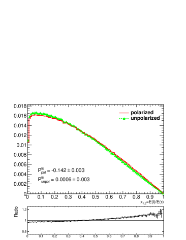
(a) $\tau\to l\nu_{l}\nu_{\tau}$

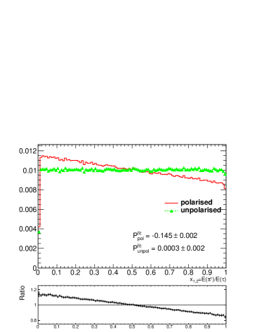
(b) $\tau\to\pi\nu_{\tau}$

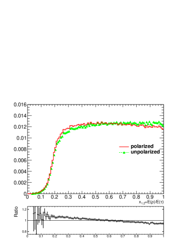
(c) $\tau\to\rho\nu_{\tau}$

Figure 1: The spectra of visible $\tau$ decay energy normalized to $\tau$ energy, $x_{1,2}$. Spin effects included (red, solid line) and neglected (green, dashed line with triangles). The $\tau$ leptons are produced through $Z$ decay close to the mass peak. The $\tau$ polarization $P$ is obtained from the fit to the distributions constructed from $Z\to\tau\tau$ sample for polarized and unpolarized (unweighted) cases. For the fit, the first bin in $\tau\to\pi\nu$ case and first five bins in $\tau\to l\nu_{l}\nu_{\tau}$ case where mass effects would be the largest, were omitted.

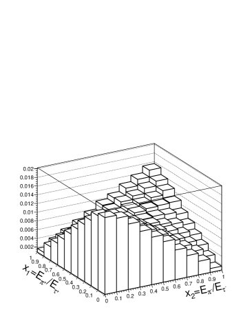
(a) $Z\to\tau^{+}\tau^{-};\;\tau^{\pm}\to\pi^{\pm}\nu_{\tau}$

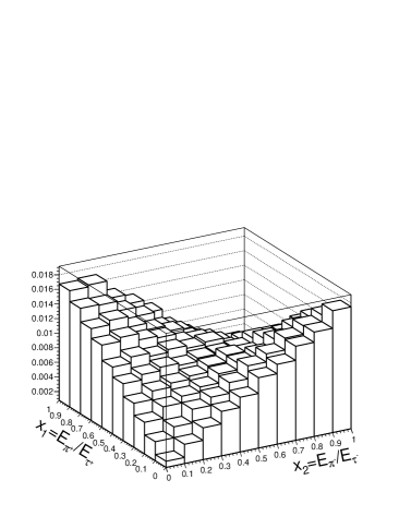
(b) $\Phi\to\tau^{+}\tau^{-};\;\tau^{\pm}\to\pi^{\pm}\nu_{\tau}$

(c) $Z\to\tau^{+}\tau^{-};\;\tau^{\pm}\to\pi^{\pm}\nu_{\tau}$

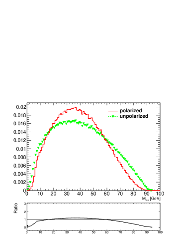
(d) $\Phi\to\tau^{+}\tau^{-};\;\tau^{\pm}\to\pi^{\pm}\nu_{\tau}$

Figure 2: The case of $Z(\Phi)\to\tau^{+}\tau^{-};\tau^{\pm}\to\pi^{\pm}\nu_{\tau}$. On plots (a, b): lego plots of $E_{\pi^{+}}/E_{\tau^{+}}\times E_{\pi^{-}}/E_{\tau^{-}}$ and on (c, d): invariant mass distributions of visible $\tau^{+}$ and $\tau^{-}$ decay products are shown. In case when spin effects are included red (solid line), otherwise green (dashed line with triangles) is used. For plots (a, c): the $\tau$ leptons produced through $Z$ decay are used. For plots (b, d): $\tau^{+}\;\tau^{-}$ pairs from spin-0 state $\Phi$ are used. All distributions are normalized to unity.

The spin effects show up differently depending on the particular $\tau$ decay channel, as shown in Fig. 1. As a consequence the spin correlation manifests itself differently depending on the particular cases of the $\tau^{+}$ and $\tau^{-}$ decay channels. In Fig. 2a and Fig. 2b we provide the two-dimensional plots (lego plots) for $Z\to\tau\tau$ events with both $\tau^{\pm}\rightarrow\pi^{\pm}\nu_{\tau}$ and the distributions of invariant mass $M_{vis}$ for the all visible $\tau$ pairs decay products combined, Fig. 2c and Fig. 2d. Note that to a good approximation $M_{vis}=Qx_{1}x_{2}$ where $Q$ denotes mass of the $\tau$-pair. In case of spin-0 state $\Phi$, the fast-fast ($x_{1,2}>0.5$) and slow-slow ($x_{1,2}<0.5$) pairs of $\pi^{\pm}$ are disfavoured, whereas in $Z/\gamma^{*}$ case the fast-slow and slow-fast configurations are less populous. Each configuration of $\tau$ decay channels feature different spin response pattern. We refer reader to series of the plots in Appendices collecting automatically created numerical results respectively for $W$, $Z/\gamma^{*}$ and $\Phi$ cases and different configurations of the $\tau$ decay modes. The Appendices (attached to the preprint version of our paper) represent examples of output from programs described in Section 5.

4.3 Fits to energy fractions, radiative corrections and experimental cuts

If there is no kinematical selection with resulting correction, mass corrections are neglected and QED bremsstrahlung in decays of $\tau$ and $Z\to\tau\tau$ is not present, analytic formulae for distributions of $x_{1}$, $x_{2}$ are given by simple polynomial expressions; formulae (2) and (3). These formulae can be used to fit the distributions and extract the value of polarization $P$. The fit can be performed for both, polarized and unpolarized distributions (the second ones constructed from appropriately weighted events). The values of the parameter $P$ obtained from the fit (average $\tau$ polarization) for the polarized and unpolarized distributions enables simple diagnostic if a given $\tau$ decay channel is sensitive to the spin effects. Fit errors on the parameter $P$ provide an estimate on the statistical sensitivity to the spin effects. One can evaluate statistical significance of the spin determination for the leptonic and single $\pi$ decay modes as can be seen from Fig. 1.

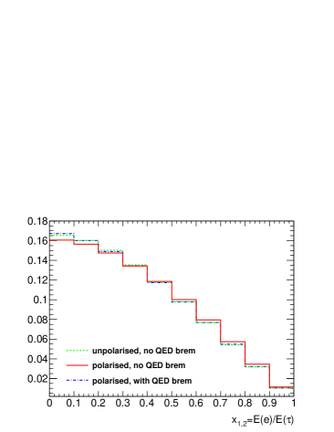
(a) $\tau\to e\nu_{e}\nu_{\tau}(\gamma)$

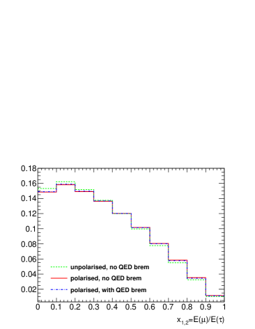
(b) $\tau\to\mu\nu_{\mu}\nu_{\tau}(\gamma)$

Figure 3: Example plots for the effects of QED bremsstrahlung in leptonic decays of $\tau$. Spectra of visible $\tau$ decay energy normalized to $\tau$ energy, $x_{1,2}$, are shown. Spin effects and QED bremsstrahlung are excluded for green (dashed line), for spin effects included but QED bremsstrahlung excluded red (solid line) and finally both spin effects and QED bremsstrahlung included blue (dotted line). Distributions constructed for $Z\to\tau\tau$ decays. Left-hand plot is for $\tau$ decays to electron, right-hand plot for $\tau$ decays to muons. For the plots, histograms were rebinned. For the fits of histograms, all 100 bins except the first five (that is exactly as in fits for Fig. 1) were used. The expression (3) was fitted to the spectra. For the $e$ channel, $P=0.004\pm 0.002,-0.141\pm 0.002,-0.015\pm 0.002$ respectively for unpolarized, polarized and polarized with bremsstrahlung effect included cases. For the $\mu$ channel, the analogous result reads $P=-0.009\pm 0.002,-0.153\pm 0.002,-0.124\pm 0.002$.

As it was explained in ref. [11], deformation of the spectra due to radiative corrections can be as big as the effect of $\tau$ polarization itself. Also our fit results given in caption of Fig. 3 support this observation. Depending on whether for calculation of $x_{1,2}$ bremsstrahlung photons are combined with the lepton or not, effect on $\tau$ polarization obtained from the fit of formulae (3) may substantially differ in size. The main deformations are for $x_{1,2}$ close to 0 or 1. In general case, when distributions are not sufficiently well described by formulae (2) and (3), Monte Carlo methods can be used to obtain the spectra and dependence on the polarization $P$ similarly to how it was done for the measurements of the $Z$ couplings performed at LEP [7].

4.4 From benchmarks toward realistic experimental distributions.

Numerical results presented above were prepared in an idealized case, where no experimental selection was applied to the analyzed samples. We have relied on the unobservable fractions of visible $\tau^{\pm}$ energies, $x_{1}$ and $x_{2}$. This is well suited for testing Monte Carlo programs and detector simulation samples. In Fig. 4, we show the impact of spin effects on experimentally observable and sensitive to spin quantity $E_{\pi^{-}}/E_{vis}$ for $\tau^{-}\to\pi^{-}\pi^{0}\pi^{0}\nu_{\tau}$ decay channel. As one can conclude effects of the spin are sizeable. The effect can be evaluated using the TauSpinner unweighting algorithm. The $a_{1}$ decay channel is less suitable for testing the programs or simulations because of more complex interpretation of different spectra. It indicates further applications, more oriented to realistic studies than the ones we have collected in Appendices for technical purposes. For applications in experimental data analysis, one should address possible complications like background contamination or limited acceptance. The template fit technique [7], convenient at LHC, as demonstrated in [4], can be used for spin in this case as well.

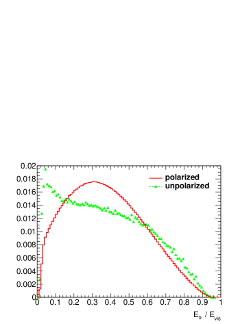
(a) $W^{-}\to\tau^{-}\bar{\nu}_{\tau};\tau^{-}\to\pi^{-}\pi^{0}\pi^{0}\nu_{\tau}$

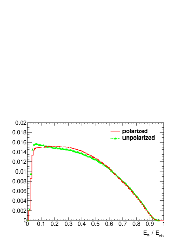
(b) $Z/\gamma^{*}\to\tau^{-}\tau^{+};\tau^{-}\to\pi^{-}\pi^{0}\pi^{0}\nu_{\tau}$

Figure 4: Example plots for effects of spin in $\tau^{-}\to\pi^{-}\pi^{0}\pi^{0}\nu_{\tau}$; the $E_{\pi^{-}}/E_{vis}$ distribution. Case when spin effects are included is denoted by red (solid line), for spin effects excluded, green (dashed line with triangles) is used. Left hand side plot is for $W^{-}\to\tau^{-}\bar{\nu}_{\tau}$ production, right hand side plot for $Z/\gamma^{*}\to\tau^{-}\tau^{+}$. Note large statistical fluctuations for unpolarized distributions in $W$ case obtained with unweighting procedure. It is because in case of 100 % polarization like for $W\to\tau\nu_{\tau}$ decays, the spin weight $wt_{spin}$ can approach zero. Its inverse used for unweighting polarization, can therefore become arbitrarily large, resulting in (integrable) singularity of the distribution. These large fluctuations indicate the limitation for use of weights method to remove spin effects from already generated events.

4.5 Consistency checks

For the TauSpinner algorithm the questions of theoretical systematic error are of a great importance. We do not plan to review this aspect of the program development now. Some results are already documented in [8, 9], but more detailed studies will be needed when the precision requirements will become more strict than presently. The work with explicit multi-leg QCD matrix elements of appropriate form, like in Ref. [22], will be mandatory.

It has been known for a long time [23, 24], that predictions for the Drell-Yan processes must lead to the dependency on the polar and azimuthal angles of outgoing leptons in the center-of-mass frame of decaying resonance in the form of second order spherical harmonics. This feature leads to the broad spectrum of possible applications, from validating implementations of higher order QCD corrections in the Monte Carlo programs, to the indirect measurement of the mass of the W boson [25].

For shown here new tests, it is important to notice that in the process of preparing spin weights, TauSpinner calculates all ingredients of the effective Born parton level cross section, as described in [10, 11, 12, 15]. Predictions for other observables or quantities of phenomenological interest, such as quark level forward-backward asymmetry or probability of a given quark flavour to originate a particular hard process event, can be obtained when executing the code. Because of mentioned above properties of QCD, formulae for polarization and other quantities, remain essentialy as at LEP.

If the studied sample is generated by the Monte Carlo program and physics history entries (flavours and momenta of quarks entering hard process) are stored, one can directly use this information to retrieve properties of the electroweak matrix elements and hadronic interactions of the studied events sample to validate precision of the TauSpinner algorithms. The four-momenta and flavours of the incoming quarks can be used to calculate parton level forward-backward asymmetry or rate of production from distinct quark flavour. These results can then be compared with the similar quantities estimated from the weights calculated by the TauSpinner algorithms using kinematics of the $\tau$ decay products only, providing very interesting test on the precision of TauSpinner algorithms.

Unfortunately information on four momenta and flavours of incoming quarks is usually available only for Monte Carlo with parton showers based on the leading logarithm approach. At the next to leading logarithm level [26] such information may be available as well, but it is not necessarily the case. One should mention here that because of the spin-1 nature of objects decaying to pair of leptons, the angular distributions of $\tau$ leptons in the rest frame of $\tau$ pair are described by spherical harmonics, of at most the order of two. This explains why higher order QCD corrections, contributing higher than second order spherical harmonics, must be small [23].

We have prepared following tests, supplementary to the ones of subsection 4.2, which exploit physics history entries. These tests may be particularly interesting if some kind of inconsistency is found in the analyzed sample and one is debugging its origin:

1. Test of kinematic reconstruction. In TauSpinner, to evaluate $\tau$ scattering angle $\theta^{*}$, an algorithm described in [27] is used. Resulting $\cos\theta^{*}$ is compared with $\cos\theta$ of scattering angle calculated from physics history entry of the event record. The difference of the two results is monitored.

2. Test of electroweak Born cross section. For the sample featuring physics history entries, the scattering angle of the outgoing lepton in the hard process can be calculated and appropriate angular distribution plotted separately for each flavour of incoming quarks. This distribution, in the leading log approximation have functional form ($1+\cos^{2}\theta+A\cos\theta$). Coefficient in front of $\cos\theta$, defining size of forward-backward asymmetry $A_{FB}$, can be obtained from the fit of this function to $\cos\theta$ distribution obtained from the analysed sample. The same coefficient can be calculated with the help of TauSpinner algorithm. This calculation uses as an input information of parton density functions (PDFs) which is convoluted with the parton level matrix-element of the hard process. The average value of the coefficient $A$ (defining size of the forward-backward asymmetry $A_{FB}$) can be therefore obtained independently from the algorithm responsible for calculating spin weights and in particular scattering angles. The comparison of the results obtained from the fit to $\cos\theta$ distribution constructed from physics history entries of the events on one side, and of TauSpinner internal calculation of $A$ (when only PDFs and virtuality of $\tau$-pair is used) on the other side, provides tests for effective Born parameters consistency in the analysed sample and TauSpinner code. Results of this test depend also on the choice of PDFs and on the correctness of the TauSpinner algorithm for reconstruction of PDFs arguments (fractions of proton momenta carried by partons) from the kinematics of the $\tau$’s (used is virtuality and pseudorapidity of the $\tau\tau$ system).

   An example of such comparison is given in Fig. 5 for the case of Drell-Yan events with virtuality in the range of 1 - 1.5 TeV. The fit gives A= 1.617 +/- 0.002 for up quarks and A= 1.692 +/- 0.003 for down quarks. From the TauSpinner calculation using Born amplitude, value of the A parameter averaged over the same sample (calculated from Born cross section) read respectively 1.613 and 1.691 with negligible statistical error . For other choices of the virtualities range agreement was found to be of a similar quality.

3. Test of PDFs. To some level, previous test can be complemented with the direct test of PDFs. Fraction of sample events (production rates) with hard process of particular incoming quark flavour can be compared with that fraction attributed by the TauSpinner algorithm. In the second case, every event contribute, but with the weight proportional to quark level total cross sections multiplied by respective PDFs. For the example shown in Fig. 5 we obtained respectively: rate of down quarks 0.217 (TauSpinner 0.216) and rate of up quarks 0.766 (TauSpinner 0.762).

The results for tests [B] and [C] depend on the PDF’s used internally by TauSpinner and on effective Born-level cross-section used at parton quark level. In case of [B] dominant contribution comes from the odd power of axial couplings, whereas in case [C] even powers of the axial couplings dominate the result. That is why the two tests are to a large extent independent.

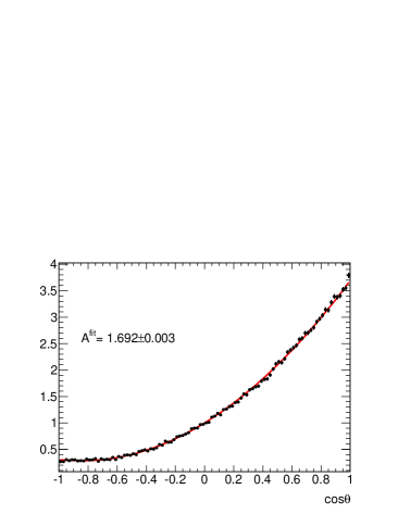
(a) $d\bar{d}\to\tau\tau$

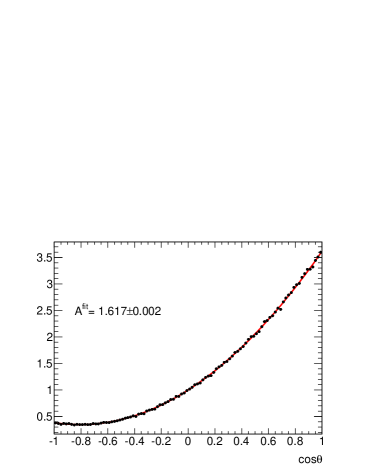
(b) $u\bar{u}\to\tau\tau$

Figure 5: Differential distribution in the hard scattering angle $\cos\theta$ calculated from physics history entries in the event record, the superimposed fit of ($1+\cos^{2}\theta+A\cos\theta$) red line is shown. Histograms are normalized to $\frac{8}{3}$ (the integral of fit function in range $[-1,1]$). The vituality of the $\tau\tau$ pair was restricted to the range 1-1.5 TeV.

1. Partial polarization test. An option that the events sample features spin correlation of the two $\tau$ leptons, but not fully the polarization effects due to production of intermediate state $Z/\gamma^{*}$ couplings is of practical interest when constructing so called $\tau$ embedded sample from $Z\to\mu\mu$ events selected from data. For example the sample features dominant spin effect, due to vector nature of the intermediate state, but is free of systematic error of the electroweak effective Born and of incoming quark PDFs. If only angular dependence of the polarization is neglected, the systematic error due to PDFs on the spin effects is reduced and much smaller systematic error due to the effective electroweak Born parameters remain. In both cases, relatively small neglected effects can be evaluated and introduced with the help of TauSpinner weights, see Section 5.4.

In the discussion of numerical results presented above, samples without any kinematical cuts were used. However, one may be interested to test how our algorithm will perform if only a particular class of events, for example of high $p_{T}$ configurations only, is used. All the tests listed above can be then performed using sub-samples defined by the particular set of cuts. In such cases, the validity of the TauSpinner algorithms and of the parton shower algorithm used for the sample generation can be explored in more exclusive phase-space regions.

4.6 Reference plots

Let us now discuss briefly the large collection of automatically created plots prepared by our testing programs. For the preprint version of our paper such plots are collected into rather lengthy appendices for the $W$, $Z/\gamma^{*}$ and spin-0 resonance $\Phi$. The distributions shown, depend on the particular sample used. We have grouped the figures for each $\tau$ decay channel (case of $W$) or for each pair of $\tau$ decay channels (case of $Z$) separately. For leptonic and single $\pi$ decay channels results of the fits to spectra (2) or (3) are given. The input samples feature complete longitudinal spin effects. The TauSpinner weights were used to unpolarize the sample. For the case of $\Phi\to\tau\tau$ events the $Z\to\tau\tau$ sample was used, but $\tau$ decays were regenerated instead of reweighted for better numerical stability.

For each type of decaying resonance, we give specification of the sample used for the respective set of plots, reporting the number of the analyzed events with the decomposition into particular (pair of) $\tau$ decay channels and initialization of the generator used for sample preparation. We also plot the control distribution of invariant mass of $\tau\tau$ ($\tau\nu_{\tau}$) system. This sanity plot verifies if the sample consists of events at the resonance peak or if substantial contribution from low energy or very high mass tails is included in the sample as well. Spin effects are different if events are taken at, above or below the $Z$ peak.

Afterwards come collection of plots to large extend following layouts of Fig. 1 and Fig. 2:

• In case of $W\to\tau\nu_{\tau}$ decay only the one-dimensional distribution of the energy fraction carried by $\tau$ lepton is plotted, comparing the case of polarized and unpolarized samples. In the captions of the plots, similarly as in Fig. 1, the fitted value of the $\tau$ polarization $P$ is given as a measure of spin sensitivity of analyzed samples.

• In the case of the $Z/\gamma^{*}$ mediated processes and for each particular combination of $\tau^{+}$ and $\tau^{-}$ decay channel, the set of histograms are collected. The first is the two-dimensional lego plot constructed from the fractions of energies of $\tau^{+}$ and $\tau^{-}$ carried by their corresponding observable decay products. Analogous lego plot is also shown for the case when spin effects are removed with the help of weights calculated by TauSpinner. Ratio of the two distributions is given in the lego plot of the second row. It demonstrates the strength of the spin effect. On the right hand side of this lego plot the one-dimensional histogram for invariant mass, of all visible products of $\tau^{+}$ and $\tau^{-}$ combined, is given. It provides a convenient way of representing spin correlation effects in case of smaller samples, which may be insufficient to fill the two-dimensional distributions. The last two plots show single $\tau^{+}$ and $\tau^{-}$ decay product spectra respectively (each plot containing original sample, sample with modifications due to TauSpinner weights and their ratio). Spectra are normalized to unity. In the captions of the plots, see Fig. 1, the fitted value of $\tau$ polarization $P$ is given as a measure of spin sensitivity of analyzed samples. Note that the groups of plots for the cases when decay channels for $\tau^{+}$ and $\tau^{-}$ are simply interchanged, coincide up to permutation of axes, unless some cuts are introduced by the user.

• In case of $\Phi$-mediated process, set of plots analogous to $Z/\gamma^{*}$-mediated processes are given.

The proposed set of benchmark plots can be extended further with the help of provided validation programs, in particular for the cases of partial implementation of polarization and spin correlations effects. Respective systematic errors can be evaluated.

5 Technical details

For the purpose of this paper, a directory TauSpinner/examples/applications has been added to the previous distributions of Tauola++. It contains several tools used to produce the plots for this paper and to obtain necessary results. It was also extended with several tests that help validate TauSpinner. If Tauola++ is configured with all prerequisites needed to compile TauSpinner package, as well as TauSpinner examples, compiling these additional programs should not require any further setup and can be done by executing make in applications directory.

5.1 The applications directory

In the following subsection we will briefly describe the sub-directories for this package and their use.

5.1.1 Generating plots

The main program, applications-plots.cxx, generates plots which are latter included in the pdf file (like of Appendix A). It uses the same algorithm as the one used in tau-reweight-test.cxx; part of the examples for TauSpinner included in Tauola++ tar-ball starting from version of November 2012. In this example code, input file events.dat is processed and for each event $WT$ weight is calculated. The set of histograms is filled with weighted (to remove spin effects) and not weighted events, separately for each $\tau$ decay mode or $\tau$ pair decay mode combination. Histograming and plotting is done using the ROOT library [21] (also fits are performed with the help of RooFit library).

This program can be used to recreate plots in the Appendices. For this, a datafile with $W$ and $Z$ which decay into $\tau$’s is needed. Note that since the template LaTeX file is prepared for both $W$ and $Z$ samples, this program can be executed on a single sample file containing both types of events or on two samples with separate $W$ and $Z$ events. Only channels $\tau\to\mu\nu_{\mu}\nu$, $\tau\to e\nu_{e}\nu$, $\tau\to\pi\nu$ and $\tau\to\rho\nu$ are analysed. To run the program:

• make sure that ROOT configuration is available through root-config,

• execute make in TauSpinner/examples/applications directory,

• verify that settings in file applications-plots.conf are correct, including the path to input file,

• execute ./applications-plots.exe applications-plots.conf.

A set of plots will be generated in the directory indicated by the configuration file (the default one is applications-plots-and-paper) and a breakdown of the $\tau$ decay channels found in the sample will be written at the end of running the program. If the input file contains both $W$ and $Z$ decays, two sets of plots will be generated, each accompanied with summary of the $W$ and $Z$ events properties. The program also saves all histograms created during processing time to out.root file. This file can be used to archive the results for further analysis or to add fits to the plots.

5.1.2 Adding fits

The code for adding fits is provided in the subdirectory applications-fits. It is built along with other programs when executing make in applications directory. This tool adds fits to the histograms generated by applications-plots.exe using the formulae (2) and (3), results of the fits are stored in the rootfile. See the README file in this directory for details on how input files are processed.

This program uses rootfiles from subdirectory applications-rootfiles. They are specified in the default configuration file applications-fits.conf as the input files of this program. The resulting plots, with added fit information on polarization, will be stored in applications-plots-and-paper directory. Previously generated plots will be overwritten. This can be changed in the configuration file with path to the output directory.

As mentioned in Section 4.3, the fit can be applied not to the whole range but to the interval $(x_{1},x_{2})$, that is why an option to perform fits only in the limited range of [$x_{\min}$,$x_{max}$] has been provided in the code and is controlled by the configuration file.

5.1.3 Recreating figures 3 and 4

The subdirectory applications-rootfiles contains rootfiles of histograms necessary to reproduce all plots shown in our paper. These rootfiles are used by applications-fits.exe. Histograms for the plots that are not part of the Appendices are also stored in the rootfiles. Executing make will invoke code to generate the plots for Figures 3 and 4. Note that generation of these rootfiles requires different setup and different data samples than for any other plots. While necessary changes are straightforward, including such options would add to the already complex structure of the validation programs, thus they were skipped in the distribution.

5.1.4 Additional tests and tools

Two additional subdirectories:

• test-bornAFB

• test-ipol

were added for further validation of the TauSpinner library. These tests are somewhat peripheral to the main topic of the paper, thus they were only documented in the README files of the corresponding sub-directories. The result of the first test is briefly discussed in Section 4.5, while the second one has not been presented here. It is, however, included in the package as a validation test of TauSpinner options (Ipol = 0, 1, 2, 3).

The applications directory contains additional programs:

• The hepmc-tauola-redecay.cxx, while not being an example for TauSpinner, can be used to process existing input file and remove $\tau$ decays substituting them with new ones generated by Tauola++. This tool can be used to generate unpolarized $\tau$ decays needed to verify different TauSpinner options (see Section 5.4). Note, that as with Tauola++, generation options are limited by the available information stored in the data files.

• The applications-comparison.cxx, uses two input files. First one is considered as a reference. For the second one TauSpinner weights are used. The same set of histograms is produced for both input files and compared afterwards. This program can be used to validate TauSpinner options, as for example in case E described in Section 5.4.

Details of how to use both programs are described in README of the directory.

5.1.5 Generating pdf file

The subdirectory applications-plots-and-paper contains the LaTeX files, as well as all other files necessary to prepare Appendices of this paper. Executing make in this directory generates the pdf file as of our paper.

Text of Appendices is stored in files: appendixA.tex and appendixB.tex. The user can thus easily re-attach results of the program run to the documentation of his own project starting from the template user-analysis.tex; the make user-analysis will include Appendices into short user-analysis.pdf.

5.1.6 Final remarks

It is possible to redo, for the sake of documenting results of one own tests, all figures and other numerical results of the Appendix A (that is also of user-analysis.pdf). In case the physics assumptions are substantially different than the one used for the present paper, shapes of the obtained distribution may differ as well. In every case the following step have to be followed:

1. generate a sample of $W$ and $Z$ decays to $\tau$; $\tau$ decaying to $\mu,e,\pi$ and $\rho$;

2. run applications-plots.exe on this sample;

3. run applications-fits.exe on the resulting rootfile and store the output in applications-plots-and-paper subdirectory;

4. execute make in applications-plots-and-paper subdirectory.

Further details on each of these steps, including more technical details on the output and input files, are given in the distribution tar-ball and in the README files located in TauSpinner/examples/applications directory and all of the sub-directories.

The numerical results of whole paper can also be reconstructed. Scripts for most of the necessary operations are prepared and documented elsewhere in the paper or in README files.

5.2 Input file formats

Essentially any HepMC [17] file (saved in HepMC::IO_GenEvent format) can be processed  Files with events stored in different format can be either converted to HepMC or interfaced using methods described in TauSpinner documentation and used in the default example tau-reweight-test.cxx.

Note that only the file applications-plots-and-paper/input-file-info.txt should be updated by the user with the information on the event sample processed. All other text files will be updated by the appropriate tools described in previous section. The content of these text files is included in the output file of pdf format, as shown in Appendix A.1.

5.3 Rounding error recovering algorithm

The $\tau$ leptons stored in data files can be ultra-relativistic. This may cause problems for the part of algorithm recalculating matrix elements for $\tau$ decays. For our example, there was no problem with errors from rounding numbers, but in general such problems are expected.

The following correcting algorithm is prepared:

1. For each stable $\tau$ decay product its energy is recalculated from the mass and momentum.

2. The four-momentum of the $\tau$ is recalculated from the sum of four-momenta of its decay products.

3. The algorithm performs check if resulting operation doesn’t introduce sizeable modifications, incompatible with rounding error recovery. If it does, a warning message is printed. This may indicate other than rounding error, difficulty with the production file. For example, some decay products not stored (eg. expected as non-observable soft photons).

The algorithm is located in file applications/CorrectEvent.h. An example of its use is provided in applications/hepmc-tauola-redecay.cxx. By default, this algorithm is turned off.

5.4 Package use cases

This package can be used to validate several TauSpinner options representing different applications of TauSpinner. Such tests include, but are not limited to:

• Applying longitudinal spin effects: adding spin effect to an unpolarized sample using weights WT calculated by TauSpinner. For this purpose, set Ipol=0 in the configuration file.

• Removing spin effects: removing spin effects from the polarized sample using weights calculated by TauSpinner. This is the default option used for our figures. The weight 1/WT instead of WT should be used.

Note, that regardless of whether Ipol=0 or 1, TauSpinner works in the same manner. The two options are distinguished at the level of the user program only (use $1/WT$ instead of $WT$ to reweight events), as shown in our demo.

• Working on the input file with spin correlations but without polarization: initialize TauSpinner with Ipol=2. In this case WT will represent correction necessary for implementation of the full longitudinal spin effects. Analogously, if the sample feature $\tau$ polarization, but polarization is missing dependence on the $\tau$ leptons directions, TauSpinner should be initialized with Ipol=3 and the missing dependence can be corrected with calculated weight WT.

• Replacing spin effects of $Z/\gamma^{*}$ with the Higgs-like spin-0 state spin correlations: This could be realized with weights ($\frac{1}{wt_{spin}}$ to remove spin effects of $Z/\gamma^{*}$ times $wt_{spin}^{\Phi}$ to introduce spin effects of $\Phi$) without modification of event kinematics. Due to large spread in the weights, this method introduces large statistical fluctuations. Alternatively, this can be realised by regenerating $\tau$ decays with Tauola++ configured for the $\tau$ pair originating from the scalar state resonance.

• Validation: test is similar to test [A], we apply spin effect to a sample without polarization. However, for this test we take the polarized sample and replace its $\tau$ decays by new, non-polarized ones using Tauola++.
  This allows to test different Ipol options as mentioned in test (C). It requires different setup and use of two input files. The TauSpinner should be executed on this new sample. The result should be then compared with the ones from original sample. Tools required to perform these steps are described in Section 5.1.4.

The results of the tests B and D are presented in the Appendices of this paper. The details of test C are described in README of applications/test-ipol subdirectory. Tools, that can be adapted to perform tests A and E, have been provided as well (see Section 5.1.4).

We have successfully performed tests A-E on samples generated with Pythia8 + Photos++ + Tauola++ (in some cases Pythia8 alone). Satisfactory results, of similar quality as discussed in our paper, sections 4.3 and 4.5 were always found. Further details for all of the cases listed above are given in the distribution tar-ball.

6 Summary

In this paper we presented the use of TauSpinner libraries for testing effects resulting from spin correlations and polarization of $\tau$ leptons in processes at LHC featuring $W$, $Z$ and $H$ decays. New example programs were developed and incorporated into program distribution tar-ball. The purpose of these programs is to analyze spin effects using information on the kinematics of $\tau$ decay products of events stored in a file. Moreover, they provide a convenient tool for validating the TauSpinner algorithms. As an important use case, this set of programs provides a method to evaluate systematic error on spin effect implementation in so called embedded $\tau$ samples, an experimental technique used for analyses at LHC experiments.

For the purpose of presenting methodology, a set of kinematical distributions was selected and the physics properties of these distributions were explained on some example plots. Event samples featuring $\tau$ lepton decays of $W$ and $Z$ production at LHC energies were generated. The weights calculated by TauSpinner algorithms were used then to remove the effects due to polarization of decaying $\tau$. The sample featuring no spin effects was also created on flight for comparisons. For studying the spin effects of the spin-0 intermediate state $\Phi$, the $Z\to\tau\tau$ sample was modified, namely the $\tau$ leptons decay products were removed and the decays were generated again, using spin density matrix of $H\to\tau^{+}\tau^{-}$ decay. The complete set of benchmark plots from analyses of these samples, graphical output from our program, is collected in the Appendices of the preprint version of our paper. What is shown in Appendix A are plots for $W$ and $Z$ decays, from executing our program on a single event file. With the additional run, one can prepare a set of plots shown in Appendix B, for the case when instead of spin effects from intermediate $Z/\gamma^{*}$ the Higgs couplings were used for the preparation of events file. As expected, effects of removed polarisation are present and spin correlations are of opposite sign to that of the $Z/\gamma^{*}$ case.

The details of the program installation and use were given. Our example provides test that algorithms of TauSpinner used for calculating spin weights are equivalent to the ones in Tauola++, the $\tau$ decay library used for creation of initial samples. We have also demonstrated how physics history entries of event samples can be used to provide validation tests for algorithm of effective Born level kinematic reconstruction and cross-section calculations used in TauSpinner.

The easiest case to understand are the spin effects of $\tau^{\pm}\to\pi^{\pm}\nu_{\tau}$ decays. The spectra are affected by spin as discussed in ref. [10, 12], that is why we have frequently used this decay channel for the example plots of the paper. Due to $Z$ polarization there is clearly identifiable slope for the $\pi^{\pm}$’s energy spectrum. The spin correlations of the two $\tau$’s disfavour configurations when one of the $\pi$ is hard and the other one is soft. For the $\Phi\to\tau\tau$ case the spin correlations effect is opposite.

For other $\tau$ decay channels, effects of spin are more complex and we have presented results in the main body of the paper only for the $\tau$’s of polarization originating from $Z\to\tau\tau$ decays. Pattern of spin correlations and single $\tau$ polarization effect depends on the $\tau$ decay channel. One can easily notice from the lego plots that it will be affected by the kinematical selection on the other $\tau$ decay products as well, biasing the observed $\tau$ polarization.

One should keep in mind when performing above tests that features of presented distributions depend strongly on the analyzed event sample. If $\tau$ leptons predominantly originate from the decays of $Z$, $W$, or $H$, of virtualities close to the resonance peaks, and with the spin effects taken into account, the distributions should be similar to the ones presented in this paper. However, it might not always be the case. For results presented in this paper parameters of the electroweak interactions and the PDFs used were carefully tuned between events generation and TauSpinner analysis codes. If this is not the case particular patterns of discrepancies may appear. We will investigate this point in the future.

To evaluate sensitivity to the spin the average $\tau$ lepton polarization fits to the histograms of the simple analytic distributions are provided. The effects of QED bremsstrahlung or mass corrections are not incorporated into the functions used for fits in case of leptonic $\tau$ decay. At LEP [11], it was shown that they may be of the similar size and shapes as polarization effects. We have also discussed that the alternative to analytical formule, Monte Carlo based template distributions are useful for fits and evaluation of spin effects.

From the discussion presented in this paper we left aside discussion on functionality of matrix-element re-weighting like the one described in ref. [9] and recently being upgraded even further. This approach may be helpful to evaluate if spin effects present in a given sample can be helpful to distinguish different production mechanisms, ones combined with the effects of production distributions. In our present study, we however concentrated on discussing spin effects only.

Appendix A Benchmark results

The Appendix A with its subsections represents output from a single execution of applications-plots.exe program. The numerical results of the Appendix are obtained from the events file generated by run of Pythia8 combined with Tauola++, details of initialization are given later in the Appendix. For the fits, all 100 bins except the first five in $\tau\to l\nu_{l}\nu_{\tau}$ case and first one in $\tau\to\pi\nu$ case, were used.

The figures in the main part of our paper are taken from the ones of Appendices, with somewhat improved graphic style for better readability. For the plots of Fig. 1, the bottom-left plots Figs. A.5, A.8 and A.13, were selected. The lego plot (and visible mass plots) of Fig. 2 are shown as the top-left lego plots (and mid-right plots) of Figs. A.8 and B.4 respectively.

A.1 Input files

The list of files and additional information on generation of events used for the plots: input-file-info.txt

Configuration file used by the program:

input-config-file.txt

Configuration file used by the fitting program:

fit-config-file.txt

A.2 W decays

The invariant mass distribution and break-down on the $\tau$ decay channels are shown for $\tau\nu_{\tau}$-pair originating from $W$ decay. The spin effects should not depend on the virtuality of the $W$ intermediate state, but this may be not the case if New Physics samples are studied.

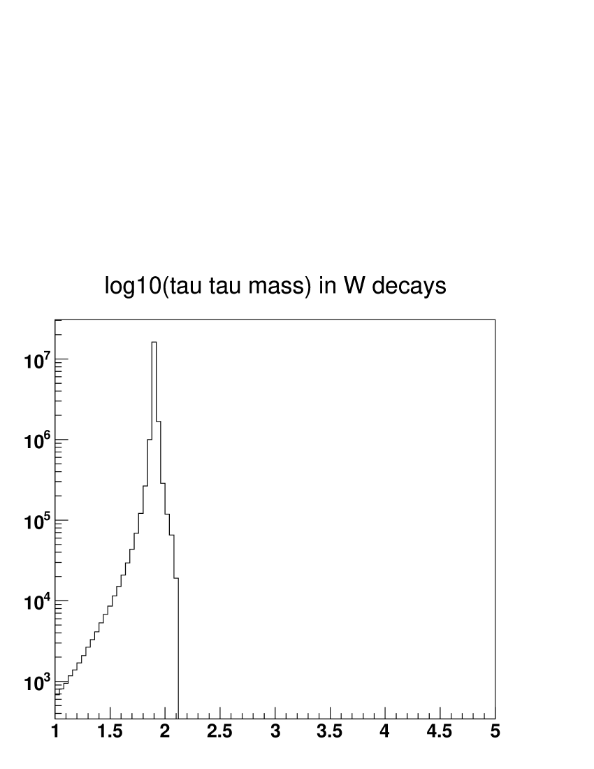
Figure A.1: Invariant mass distribution of $\tau\nu_{\tau}$-pair originating from $W$ decay.

input-W-event-count.txt

A.2.1 The energy spectrum: $\tau^{\pm}\to\mu^{\pm},e^{\pm}$

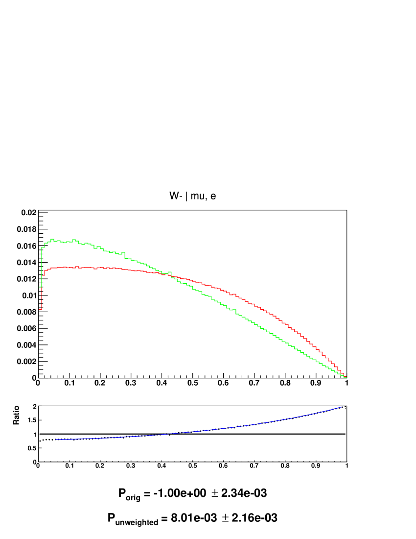
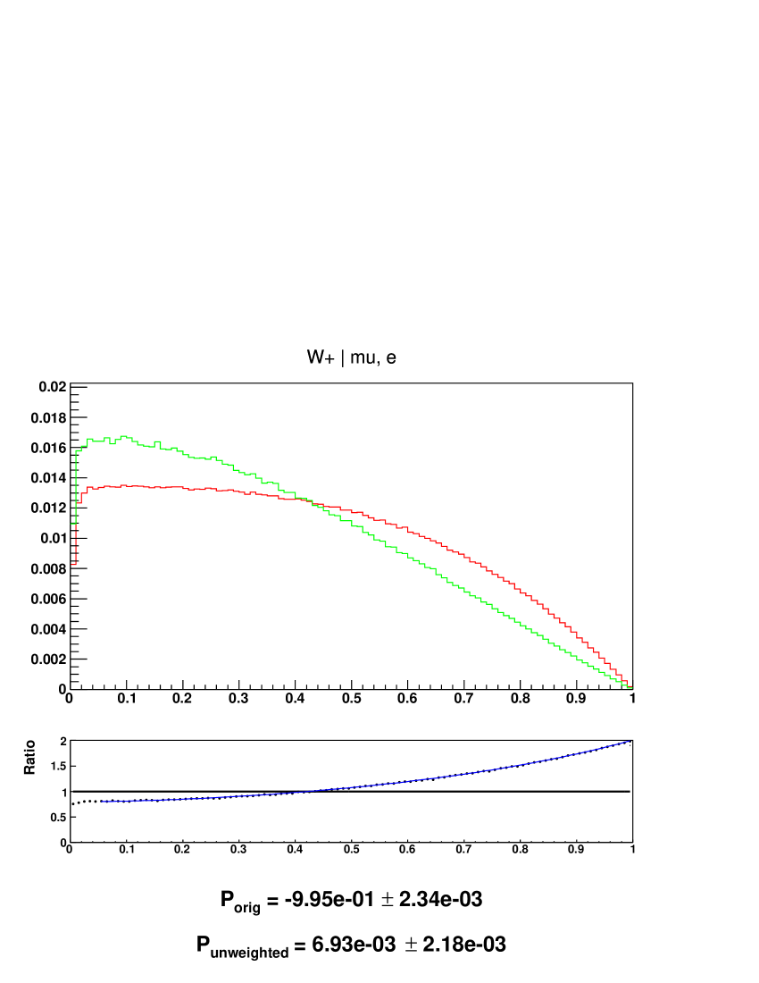
Figure A.2: Fraction of $\tau$ energy carried by its visible decay products¹⁸. Red line is for original sample, green line is for modified sample after removing polarisation using TauSpinner weights, black line is ratio original/modified.

A.2.2 The energy spectrum: $\tau^{\pm}\to\pi^{\pm}$

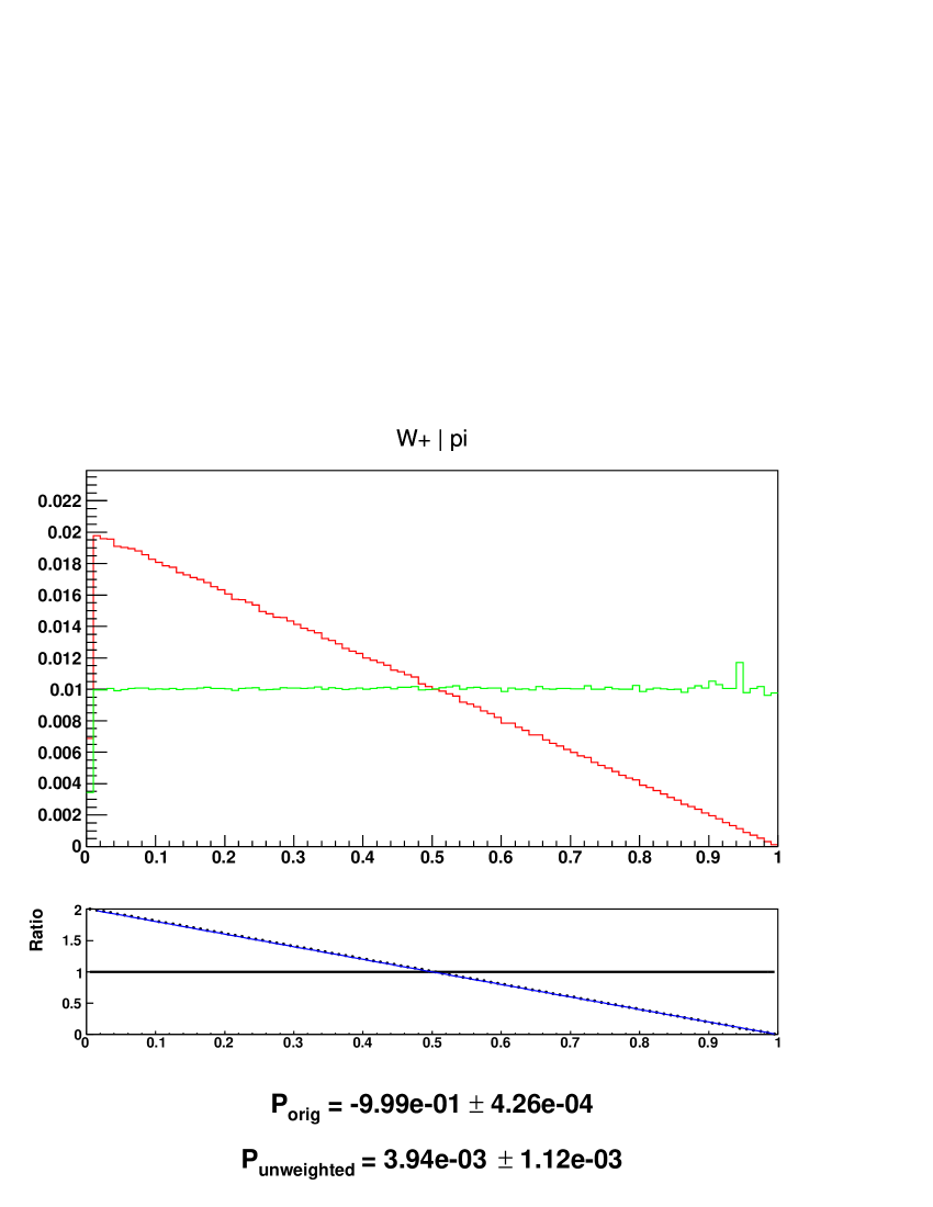
Figure A.3: Fraction of $\tau$ energy carried by its visible decay products¹⁸. Red line is for original sample, green line is for modified sample after removing polarisation using TauSpinner weights, black line is ratio original/modified.

A.2.3 The energy spectrum: $\tau^{\pm}\to\rho^{\pm}$

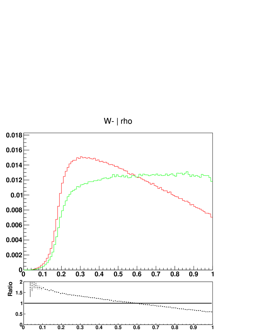
Figure A.4: Fraction of $\tau$ energy carried by its visible decay products. Red line is for original sample, green line is for modified sample after removing polarisation using TauSpinner weights, black line is ratio original/modified.

A.3 Z decays

The invariant mass distribution and break-down on the $\tau$ decay channels are shown for $\tau\tau$-pair originating from $Z$ decay. The spin effects strongly depend on the virtuality of the $Z/\gamma^{*}$ intermediate state. Events were generated explicitly requiring virtuality of $Z\gamma^{*}$ within 88-94 GeV window. Minor contamination from some other process is nevertheless observed (we have not traced it back).

input-Z-event-count.txt

A.3.1 The energy spectrum: $\tau^{-}\to\mu^{-},e^{-}$ vs $\tau^{+}\to\mu^{+},e^{+}$

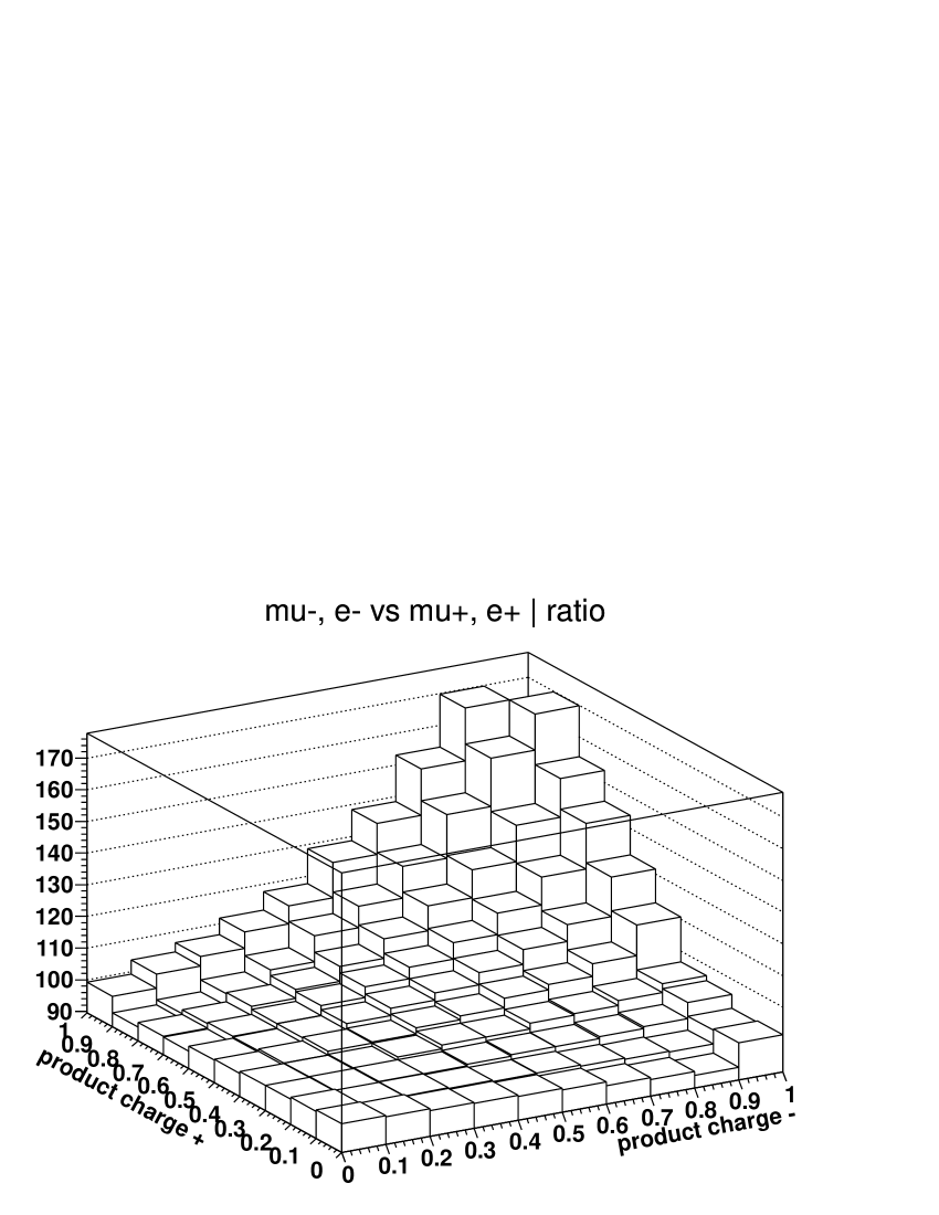
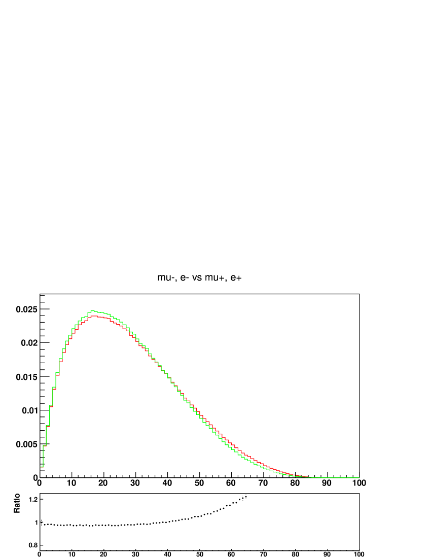
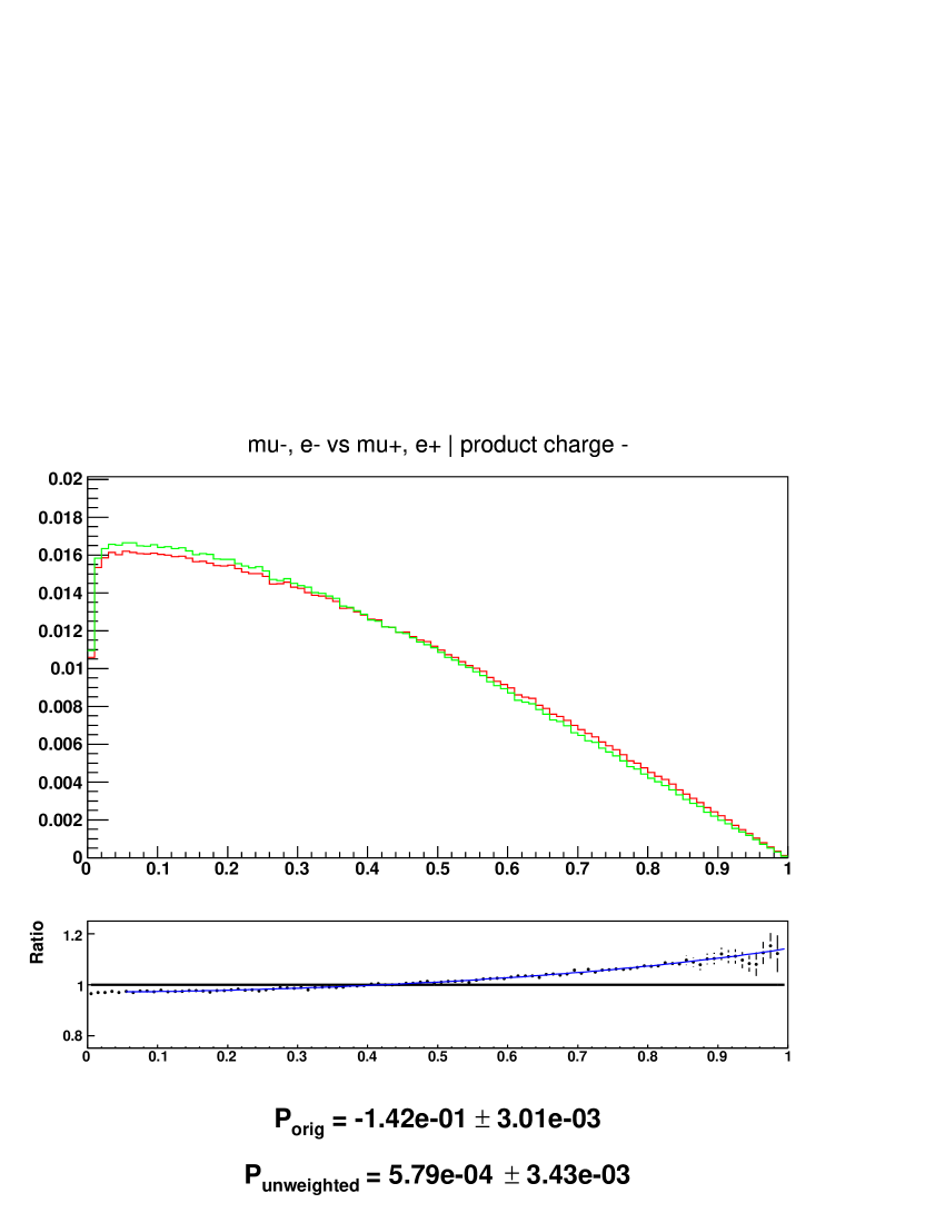
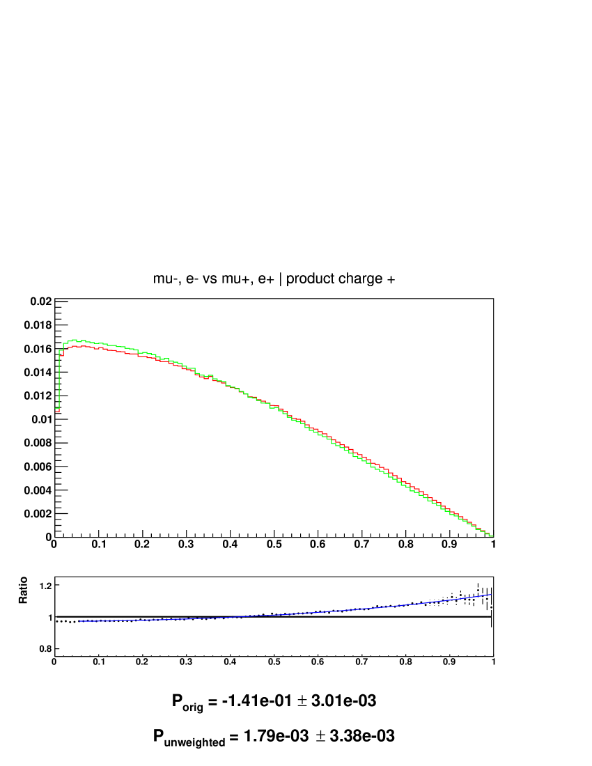
Figure A.5: Fractions of $\tau^{+}$ and $\tau^{-}$ energies carried by their visible decay products: two dimensional lego plots and one dimensional spectra¹⁸. Red line is for original sample, green line is for modified sample after removing polarisation using TauSpinner weights, black line is ratio original/modified with whenever available superimposed result for the fitted functions.

A.3.2 The energy spectrum: $\tau^{-}\to\mu^{-},e^{-}$ vs $\tau^{+}\to\pi^{+}$

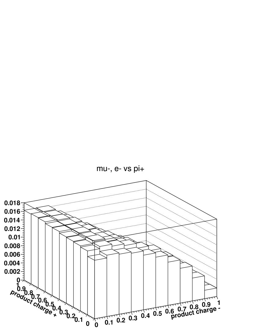
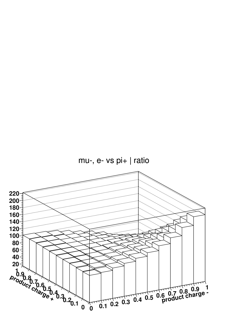
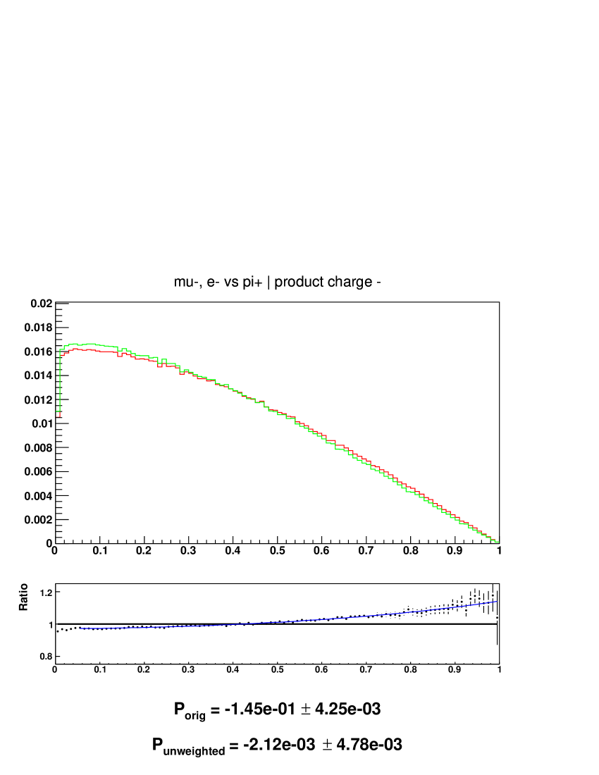
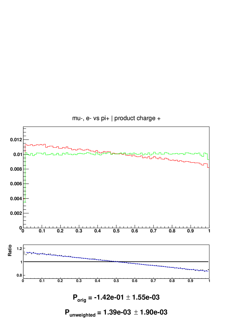
Figure A.6: Fractions of $\tau^{+}$ and $\tau^{-}$ energies carried by their visible decay products: two dimensional lego plots and one dimensional spectra¹⁸. Red line is for original sample, green line is for modified sample after removing polarisation using TauSpinner weights, black line is ratio original/modified with whenever available superimposed result for the fitted functions.

A.3.3 The energy spectrum: $\tau^{-}\to\pi^{-}$ vs $\tau^{+}\to\mu^{+},e^{+}$

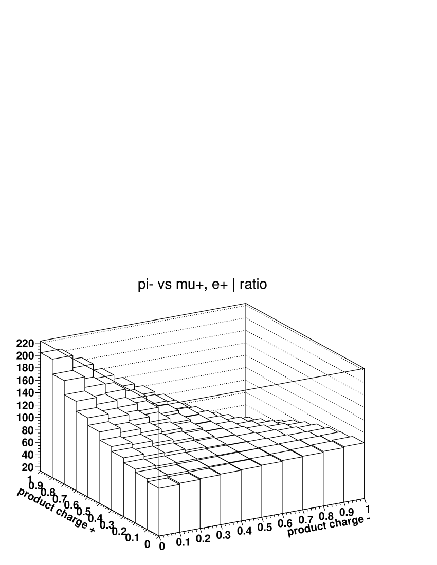
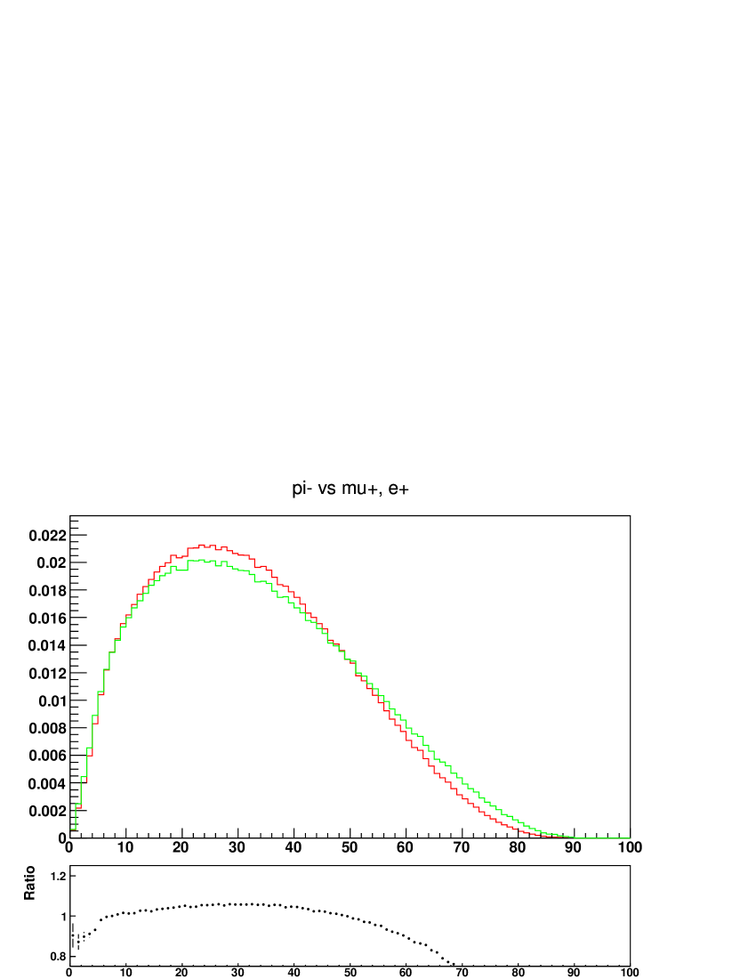
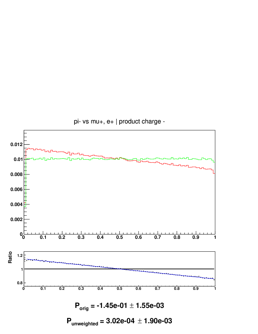
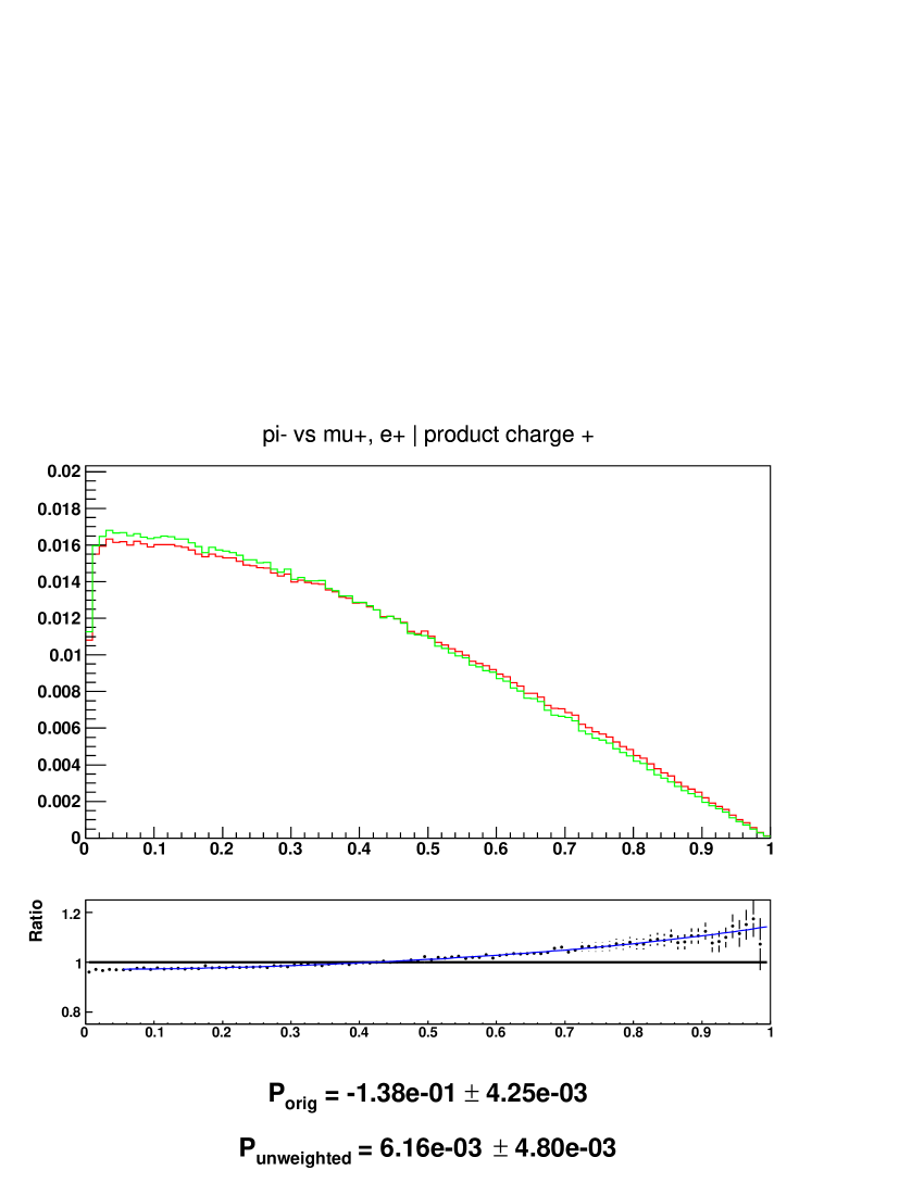
Figure A.7: Fractions of $\tau^{+}$ and $\tau^{-}$ energies carried by their visible decay products: two dimensional lego plots and one dimensional spectra¹⁸. Red line is for original sample, green line is for modified sample after removing polarisation using TauSpinner weights, black line is ratio original/modified with whenever available superimposed result for the fitted functions.

A.3.4 The energy spectrum: $\tau^{-}\to\pi^{-}$ vs $\tau^{+}\to\pi^{+}$

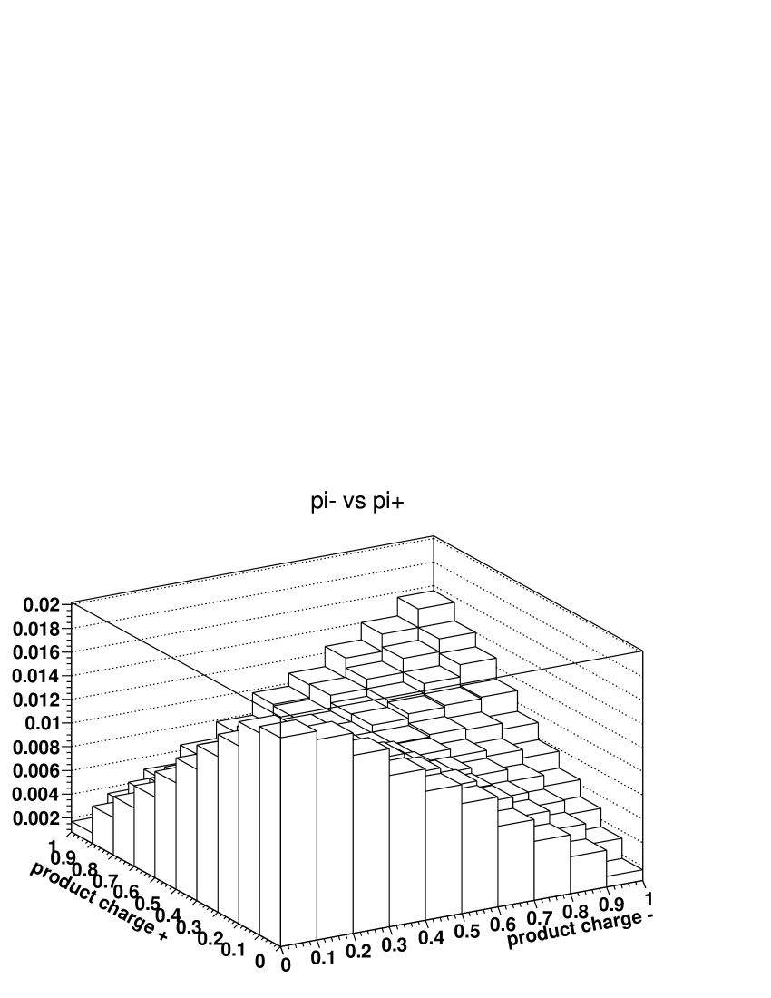
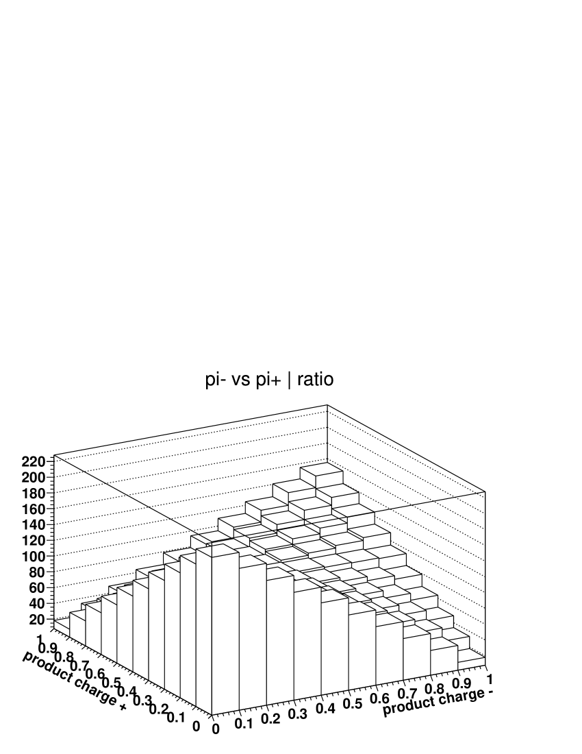
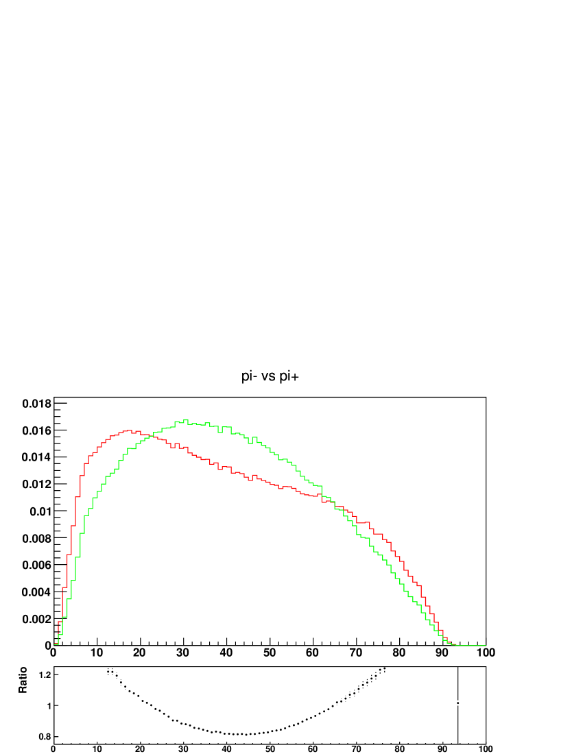
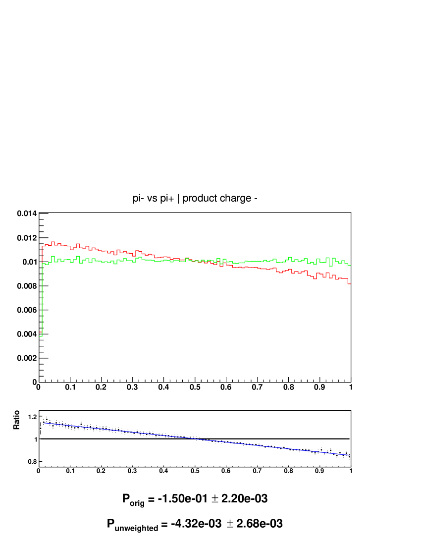
Figure A.8: Fractions of $\tau^{+}$ and $\tau^{-}$ energies carried by their visible decay products: two dimensional lego plots and one dimensional spectra¹⁸. Red line is for original sample, green line is for modified sample after removing polarisation using TauSpinner weights, black line is ratio original/modified with whenever available superimposed result for the fitted functions.

A.3.5 The energy spectrum: $\tau^{-}\to\mu^{-},e^{-}$ vs $\tau^{+}\to\rho^{+}$

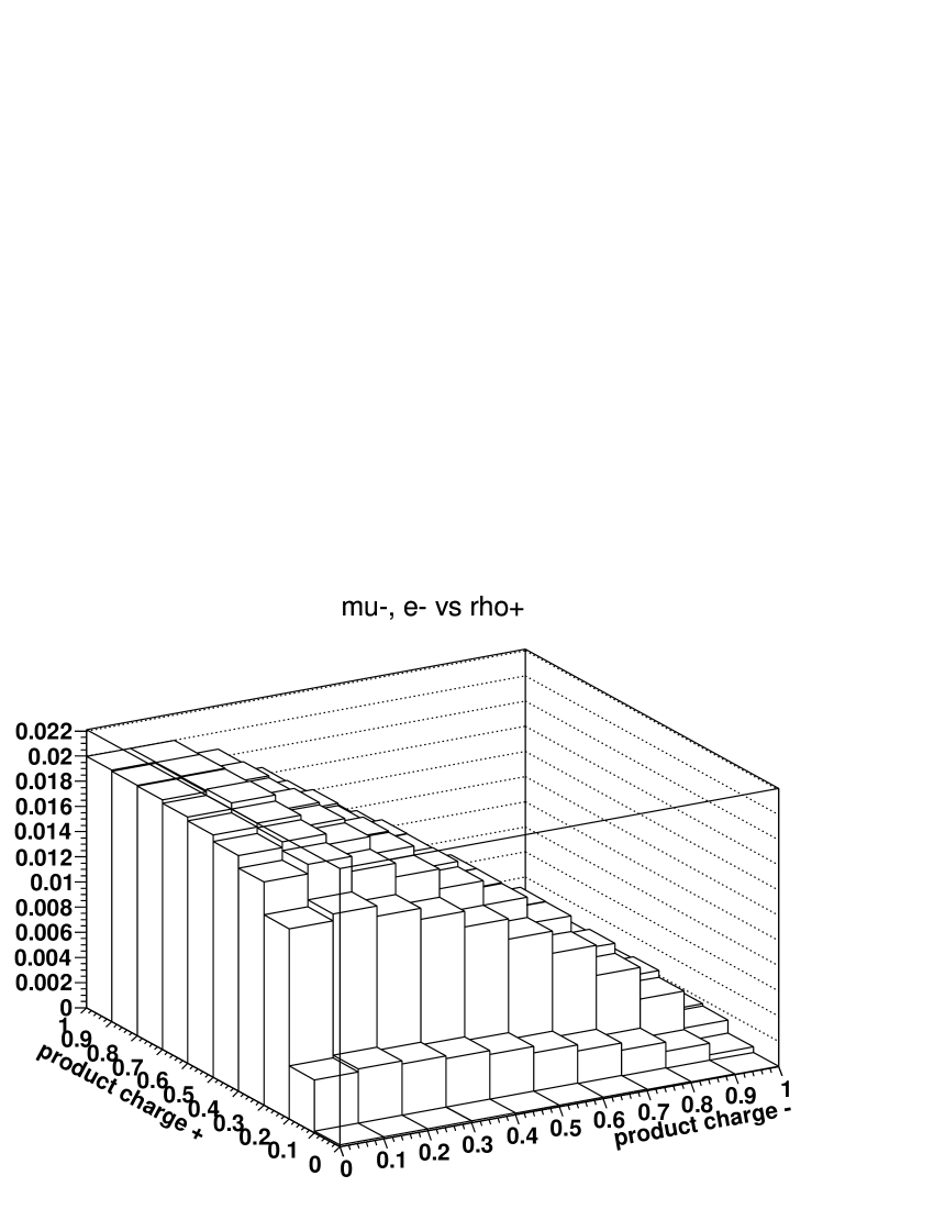
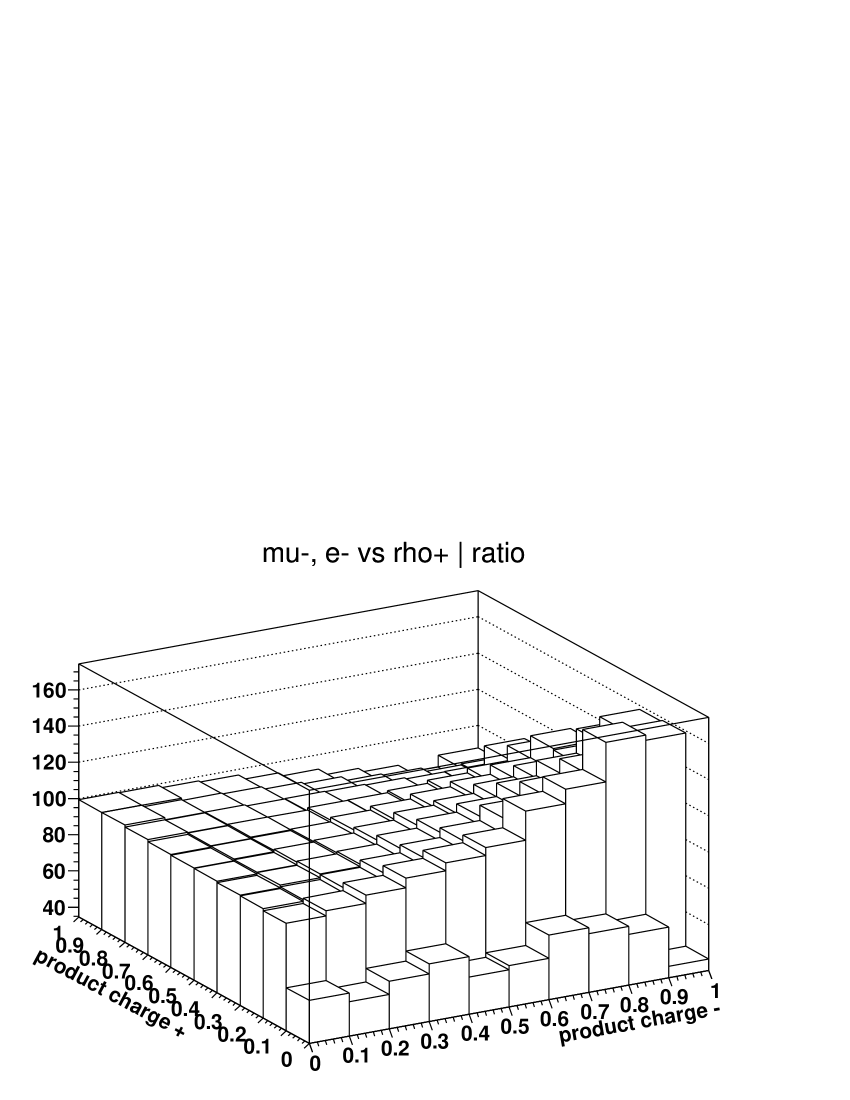
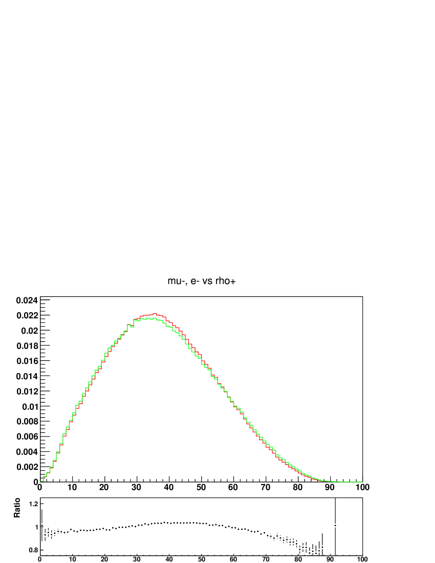
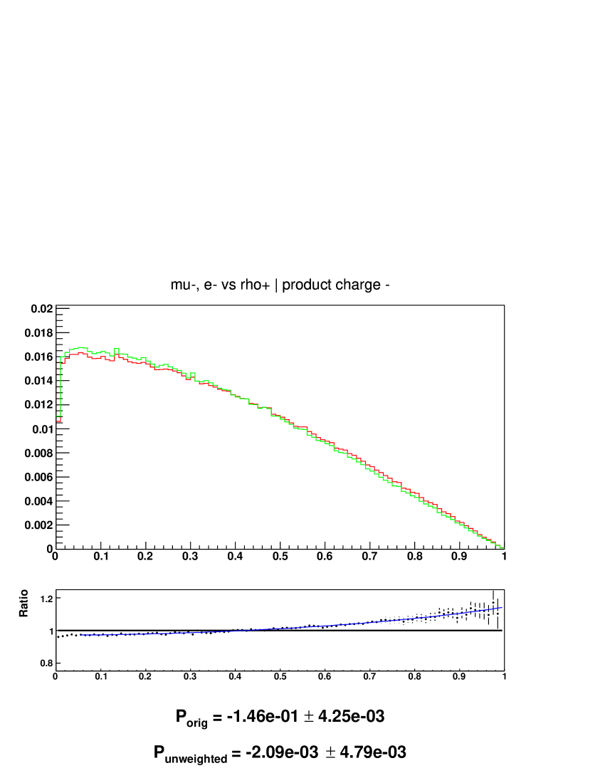
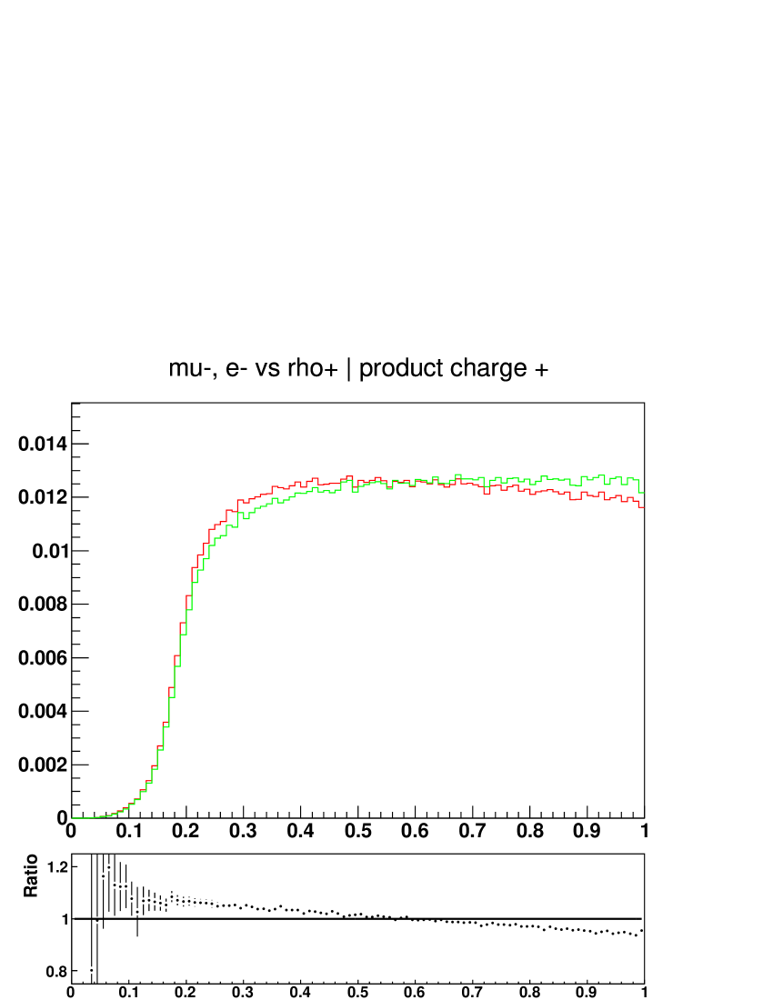
Figure A.9: Fractions of $\tau^{+}$ and $\tau^{-}$ energies carried by their visible decay products: two dimensional lego plots and one dimensional spectra¹⁸. Red line is for original sample, green line is for modified sample after removing polarisation using TauSpinner weights, black line is ratio original/modified with whenever available superimposed result for the fitted functions.

A.3.6 The energy spectrum: $\tau^{-}\to\rho^{-}$ vs $\tau^{+}\to\mu^{+},e^{+}$

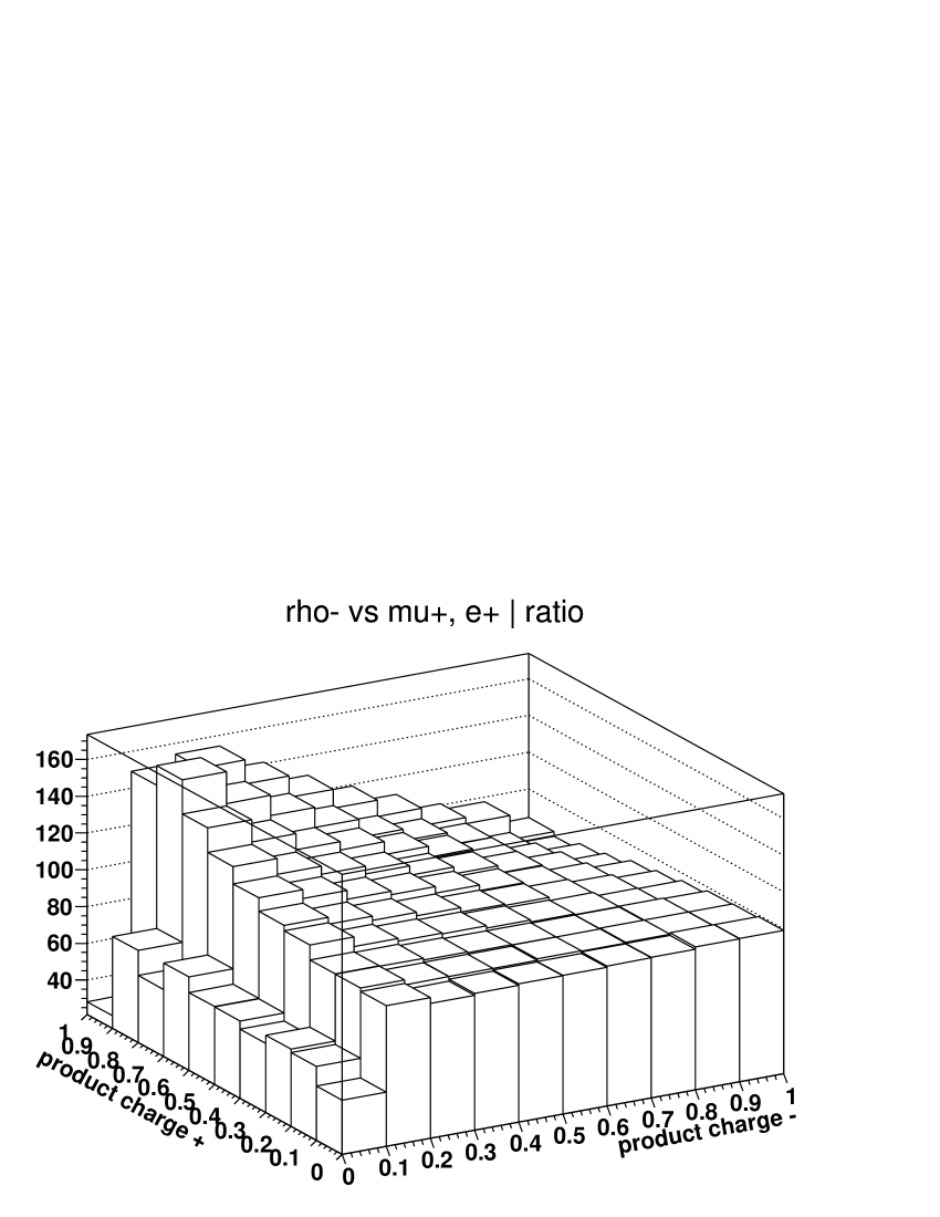
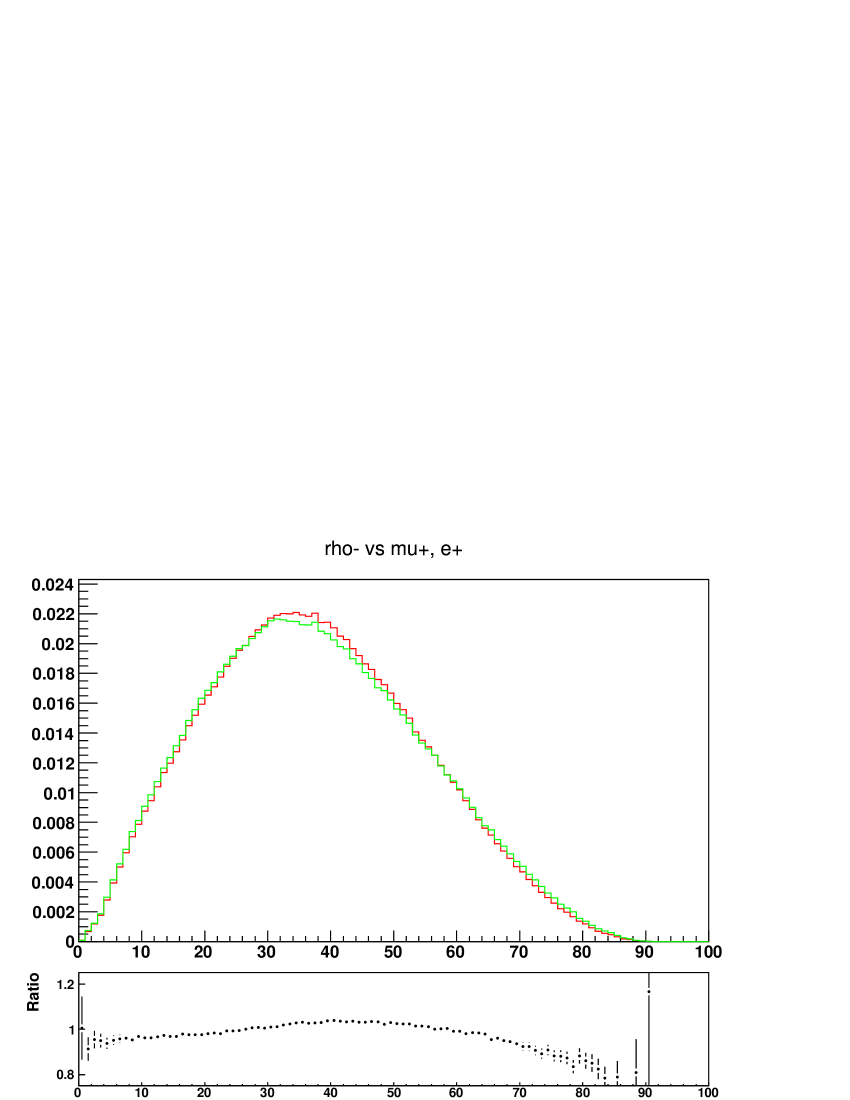
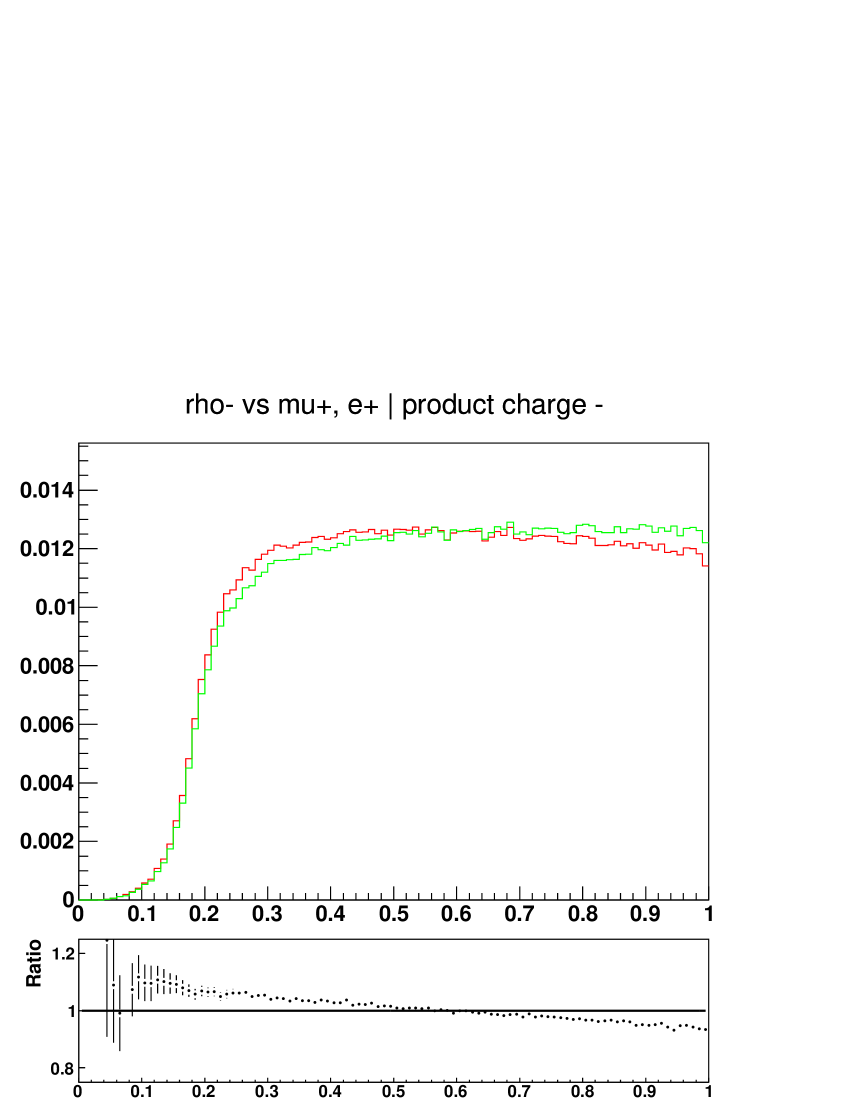
Figure A.10: Fractions of $\tau^{+}$ and $\tau^{-}$ energies carried by their visible decay products: two dimensional lego plots and one dimensional spectra¹⁸. Red line is for original sample, green line is for modified sample after removing polarisation using TauSpinner weights, black line is ratio original/modified with whenever available superimposed result for the fitted functions.

A.3.7 The energy spectrum: $\tau^{-}\to\pi^{-}$ vs $\tau^{+}\to\rho^{+}$

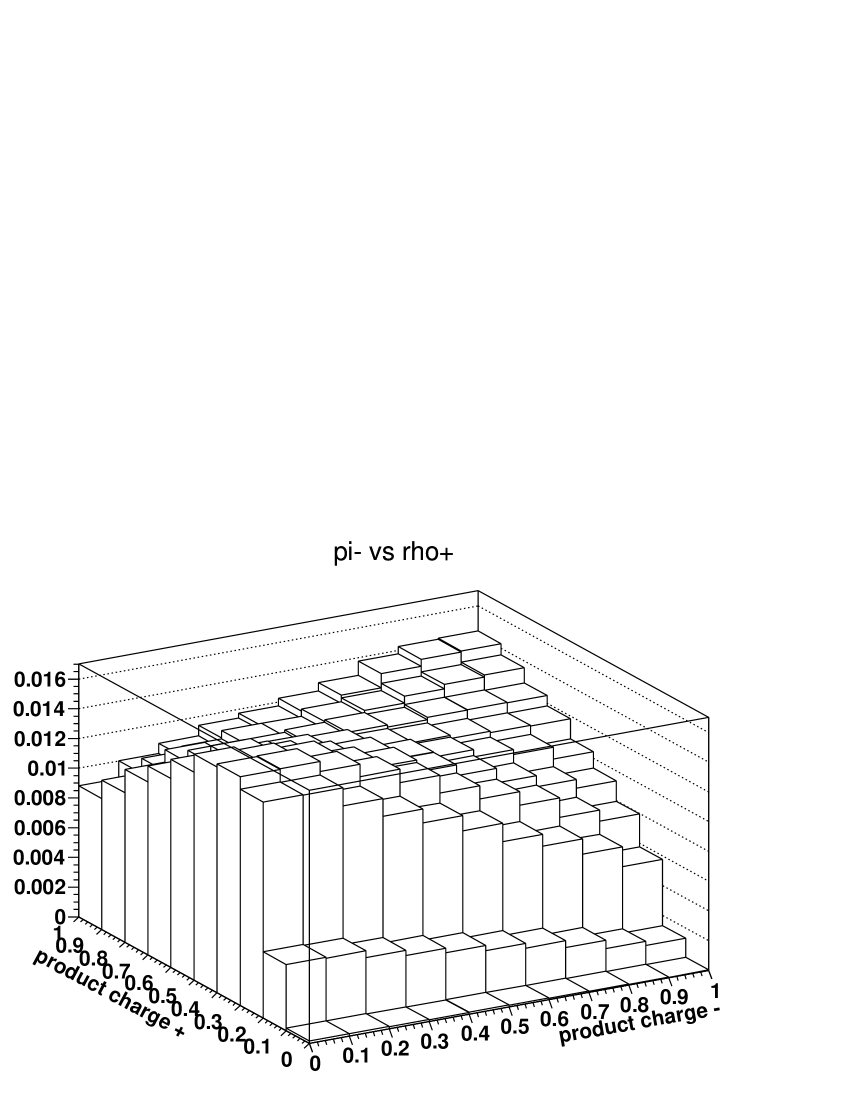
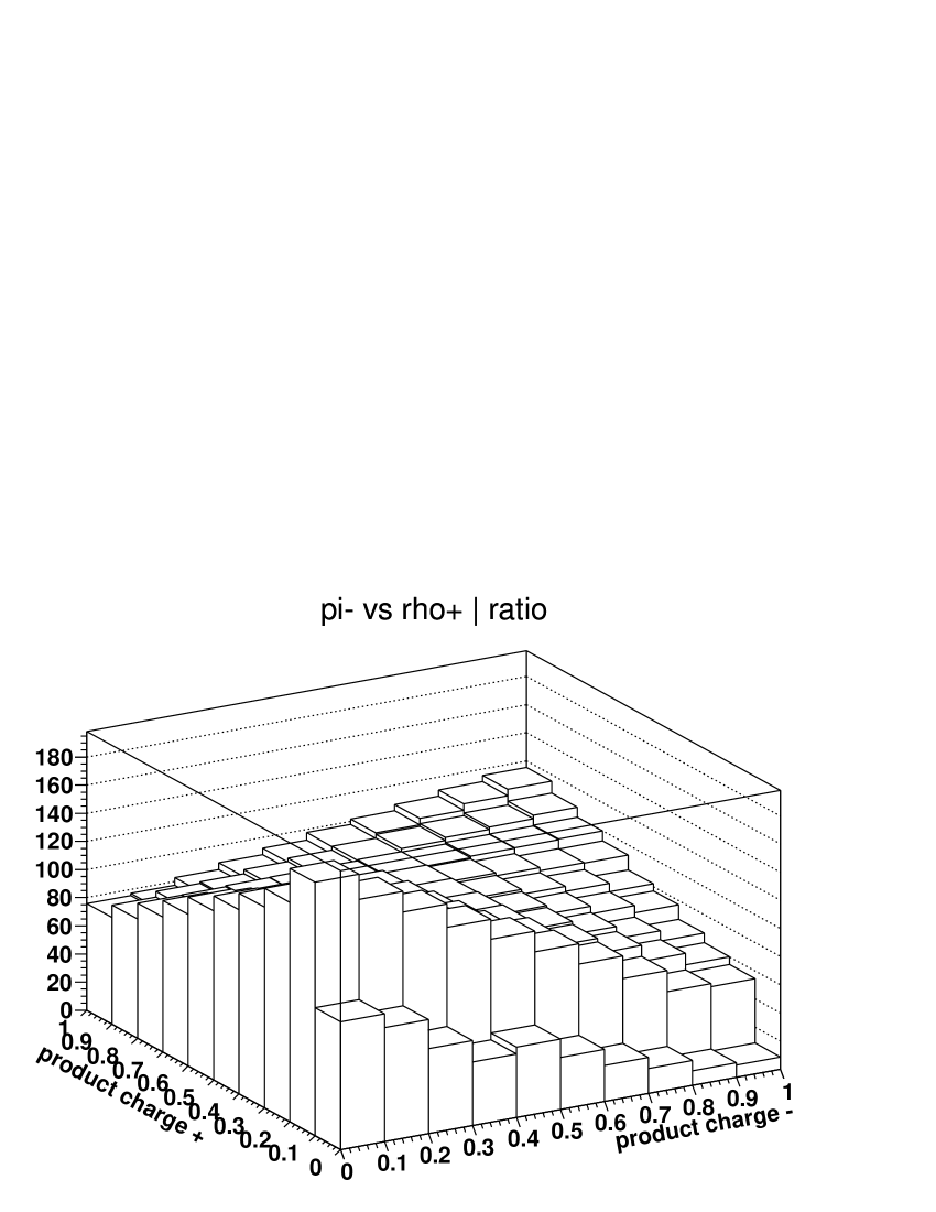
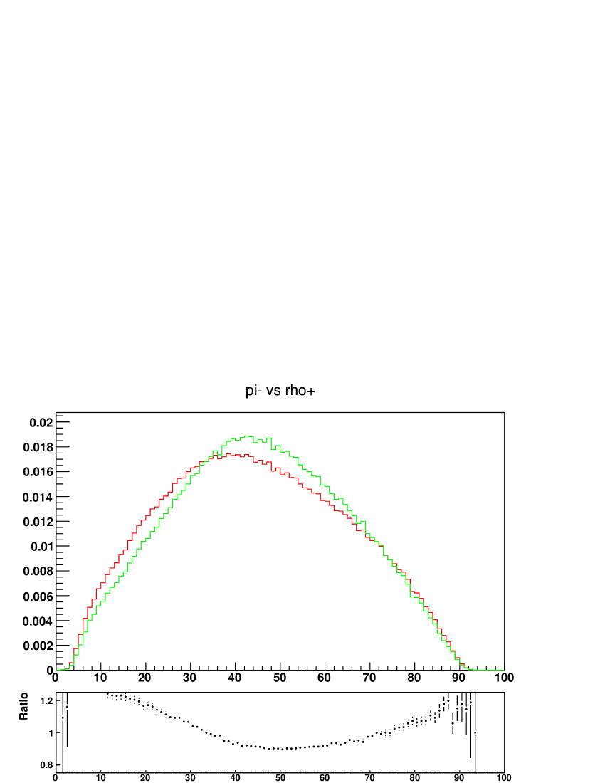
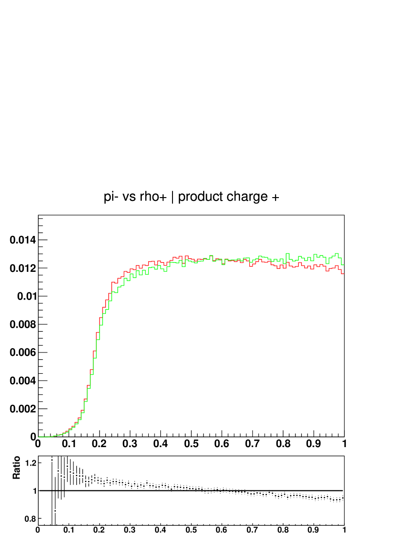
Figure A.11: Fractions of $\tau^{+}$ and $\tau^{-}$ energies carried by their visible decay products: two dimensional lego plots and one dimensional spectra¹⁸. Red line is for original sample, green line is for modified sample after removing polarisation using TauSpinner weights, black line is ratio original/modified with whenever available superimposed result for the fitted functions.

A.3.8 The energy spectrum: $\tau^{-}\to\rho^{-}$ vs $\tau^{+}\to\pi^{+}$

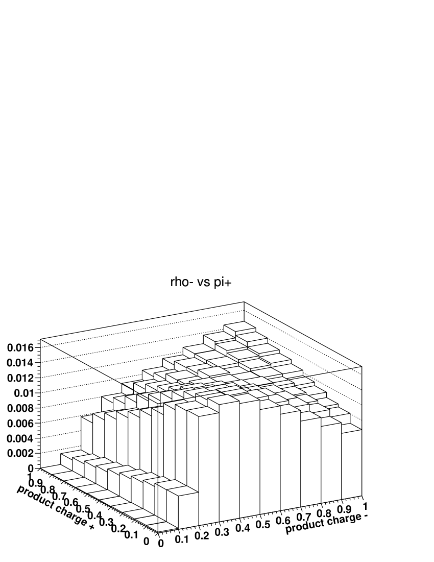
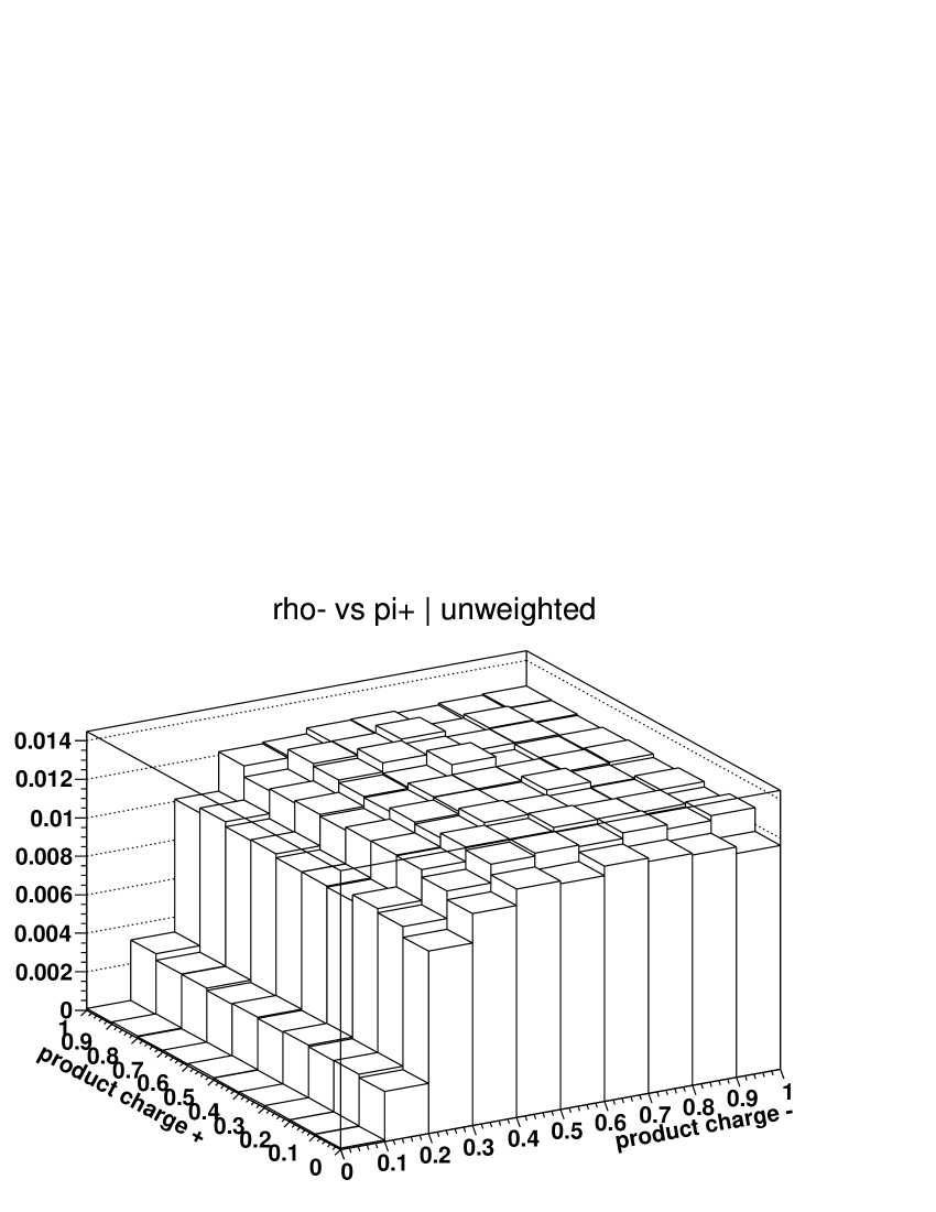
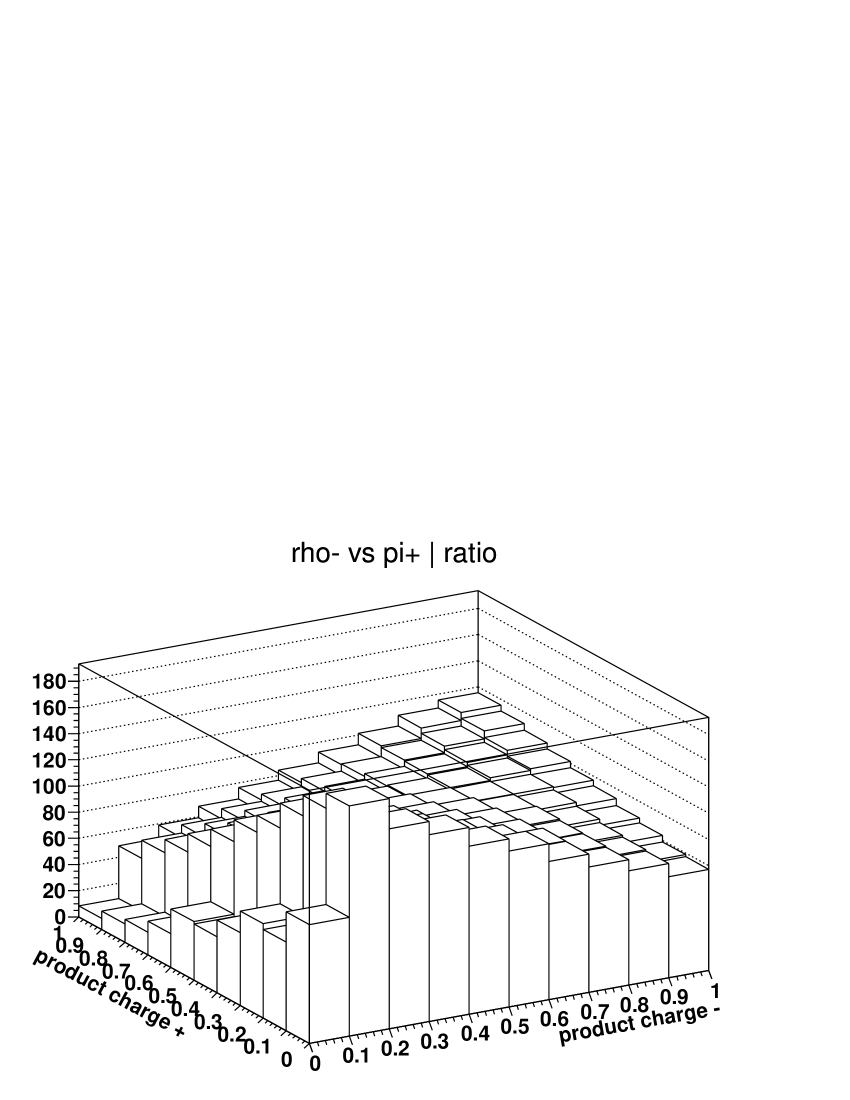
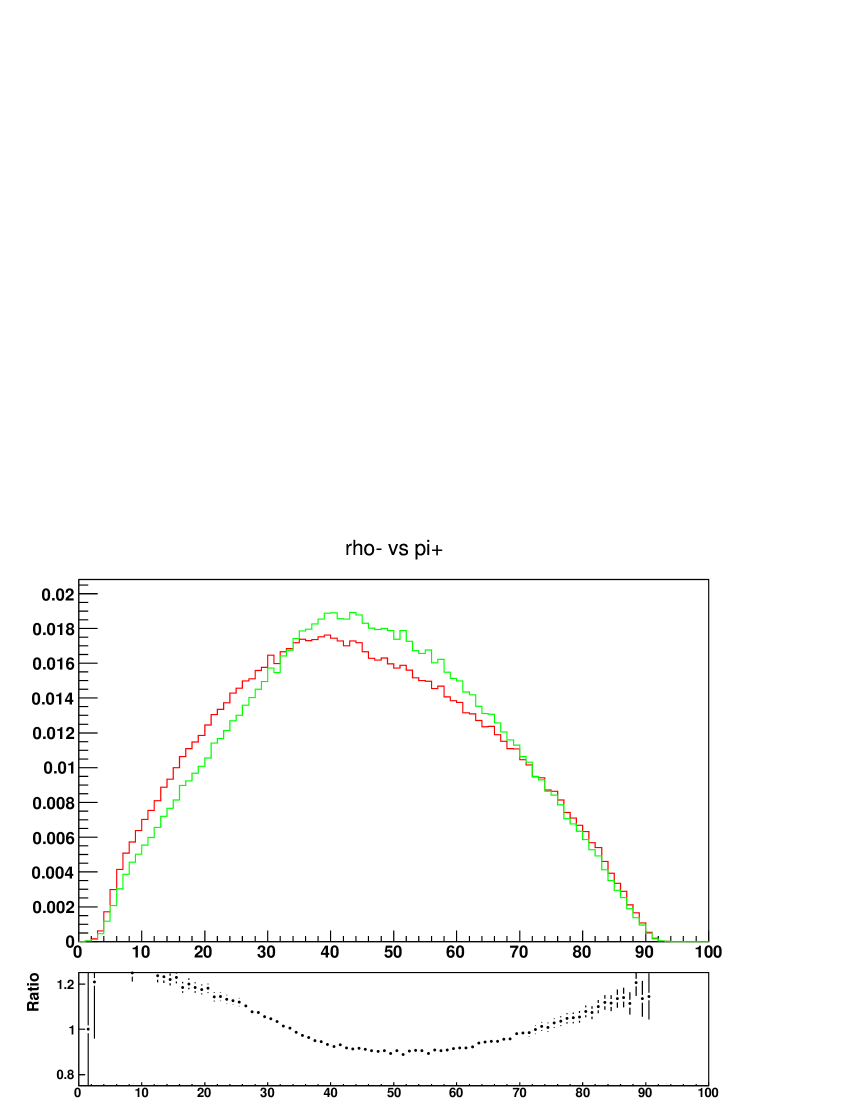
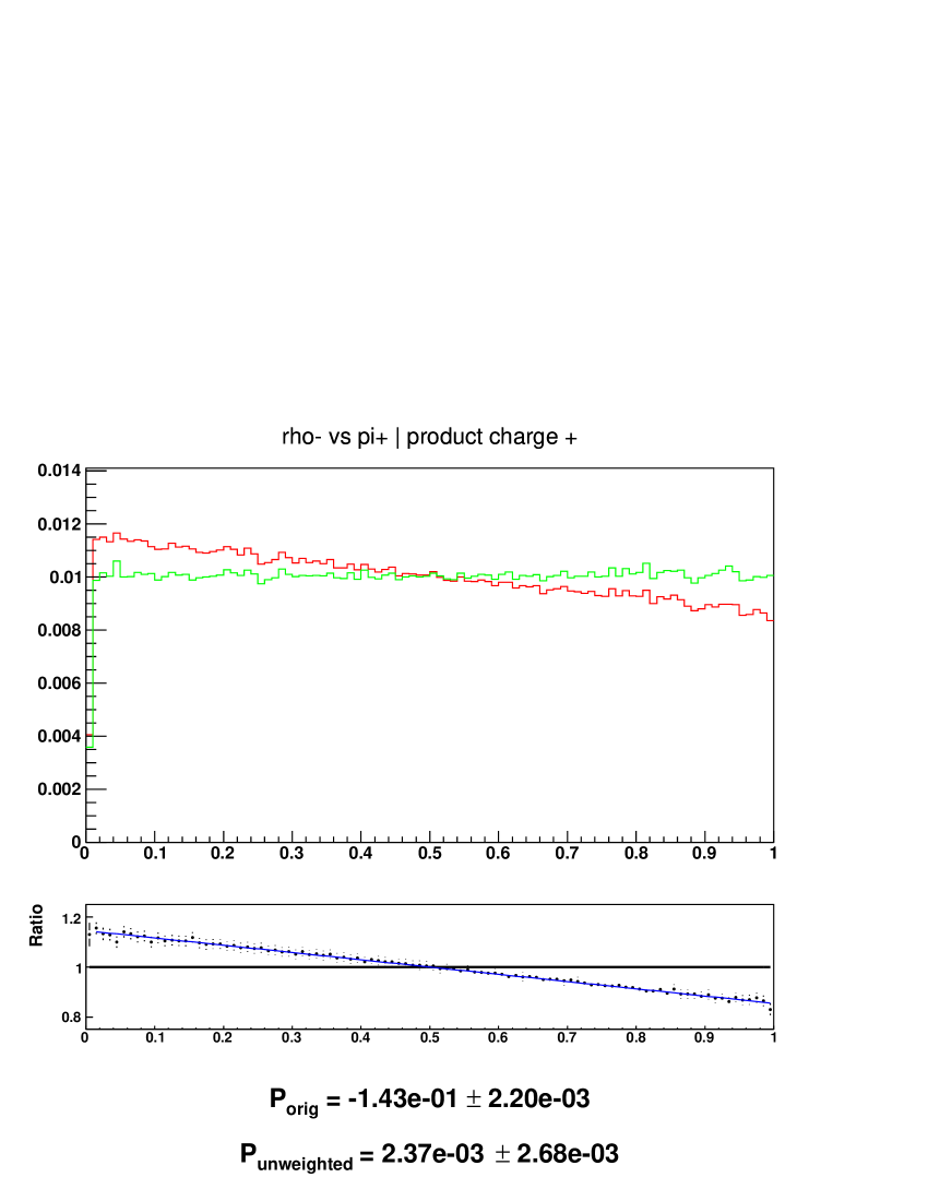
Figure A.12: Fractions of $\tau^{+}$ and $\tau^{-}$ energies carried by their visible decay products: two dimensional lego plots and one dimensional spectra¹⁸. Red line is for original sample, green line is for modified sample after removing polarisation using TauSpinner weights, black line is ratio original/modified with whenever available superimposed result for the fitted functions.

A.3.9 The energy spectrum: $\tau^{-}\to\rho^{-}$ vs $\tau^{+}\to\rho^{+}$

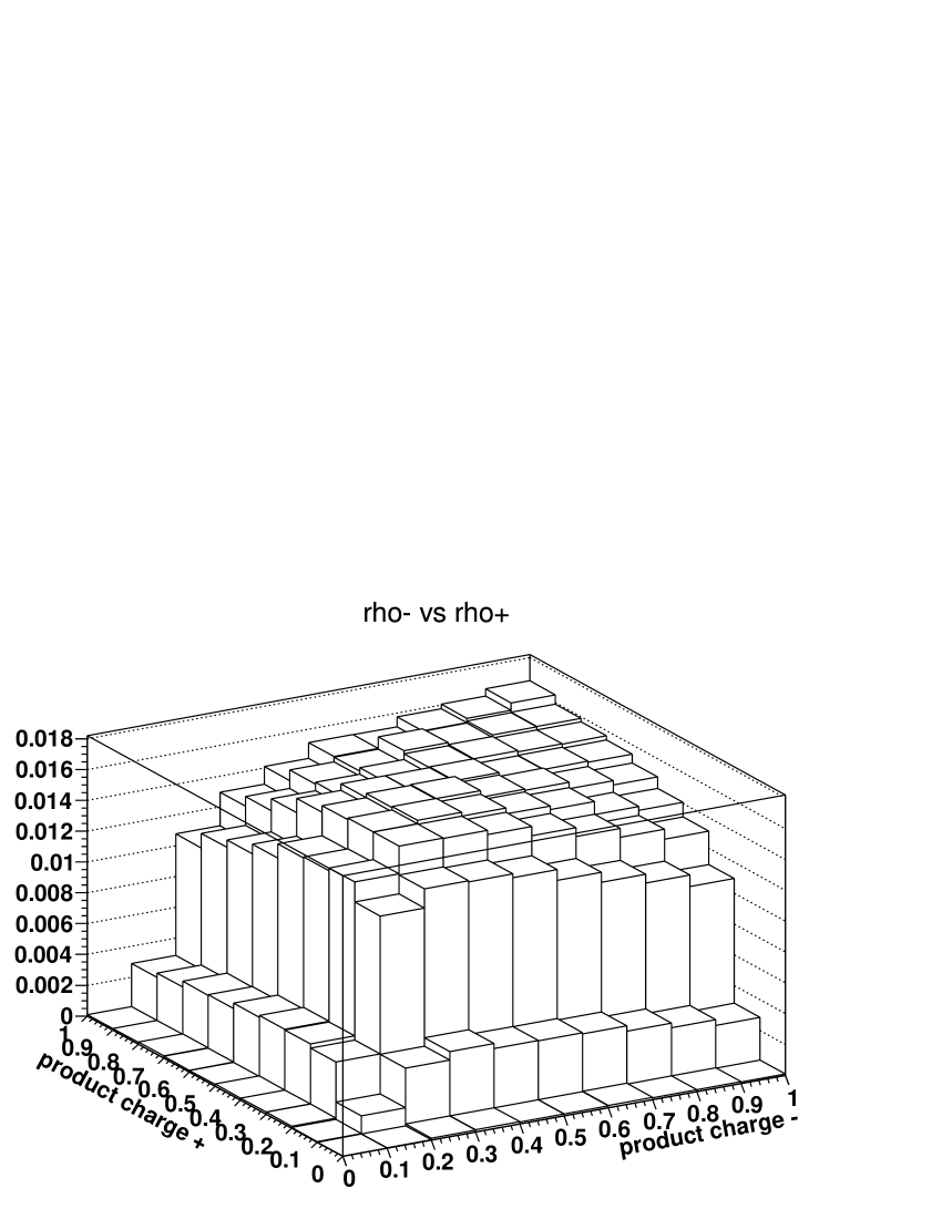
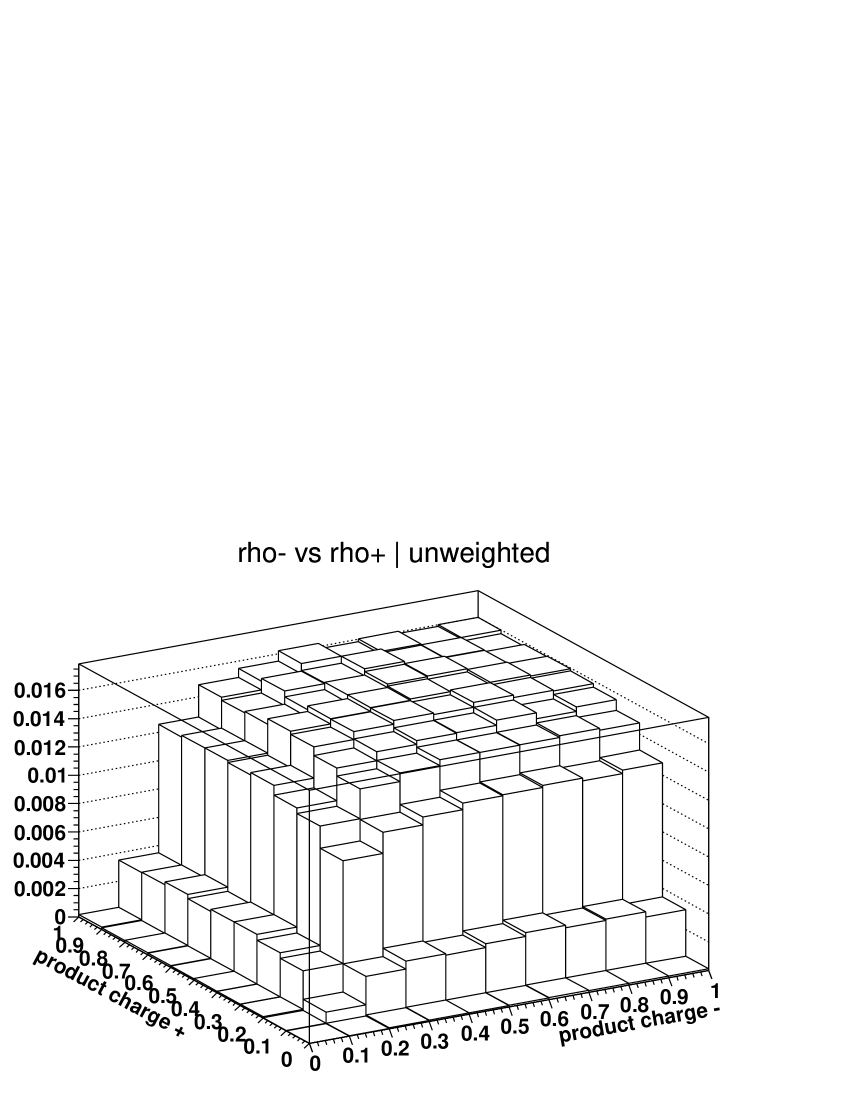
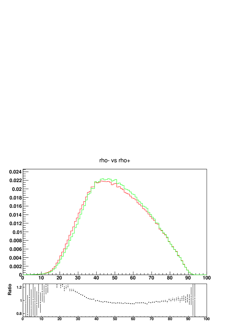
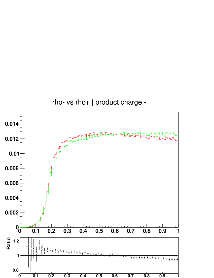
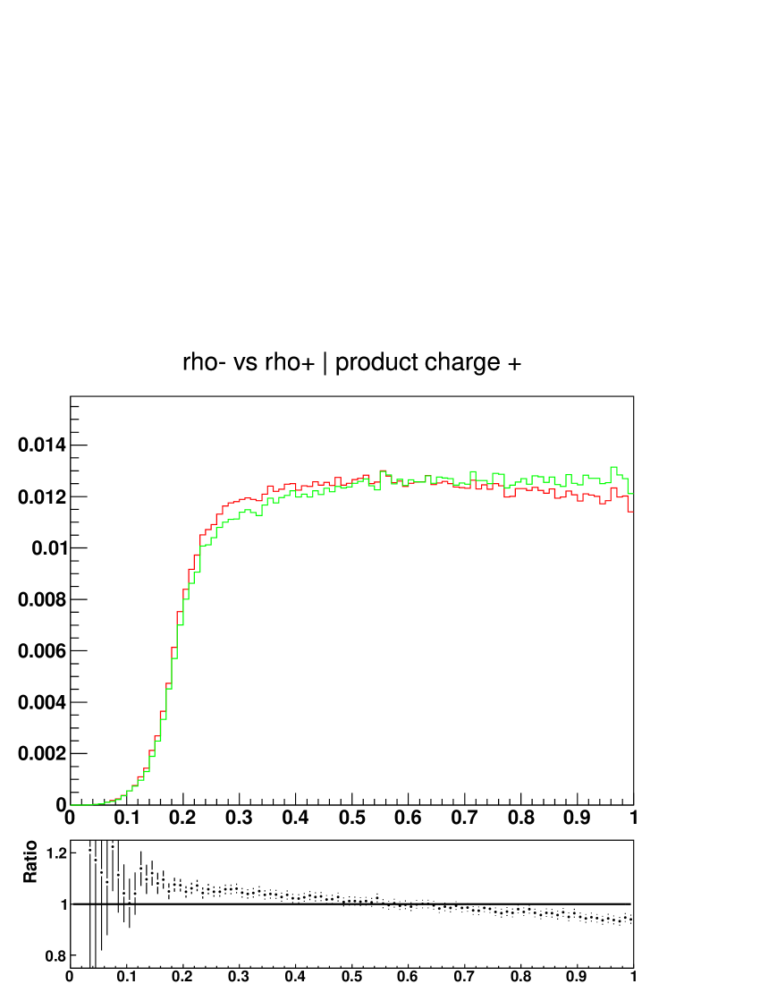
Figure A.13: Fractions of $\tau^{+}$ and $\tau^{-}$ energies carried by their visible decay products: two dimensional lego plots and one dimensional spectra. Red line is for original sample, green line is for modified sample after removing polarisation using TauSpinner weights, black line is ratio original/modified.

Appendix B $\Phi$ decays: Z decay sample but with Higgs couplings used for spin

In this section, we monitor effects of Higgs couplings for spin correlations and compare it with case of unpolarized $\tau$’s. As expected, one can observe strong opposite sign as in $Z$ case, spin correlations, and there is no effect on single $\tau$ decay product spectra.

The invariant mass distribution and break-down on the $\tau$ decay channels are shown for $\tau\nu_{\tau}$-pair originating from $\Phi$ decay. For this purpose $Z\to\tau\tau$ events were used, with $\tau$ decay products removed and $\tau$ leptons decayed again using configuration of Tauola++ like for $H\to\tau\tau$ decay. For the fits, all 100 bins except the first five in $\tau\to l\nu_{l}\nu_{\tau}$ case and first one in $\tau\to\pi\nu$ case, were used.

input-Phi-event-count.txt

B.1 The energy spectrum: $\tau^{-}\to\mu^{-},e^{-}$ vs $\tau^{+}\to\mu^{+},e^{+}$

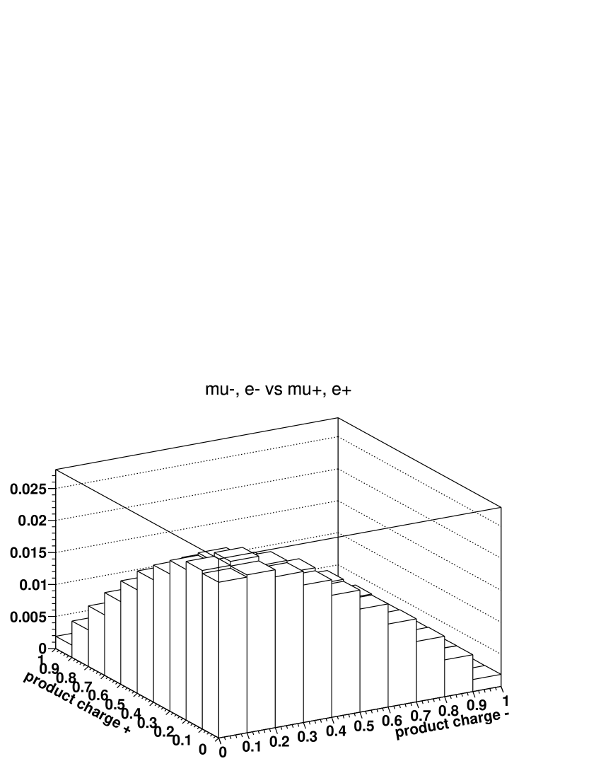
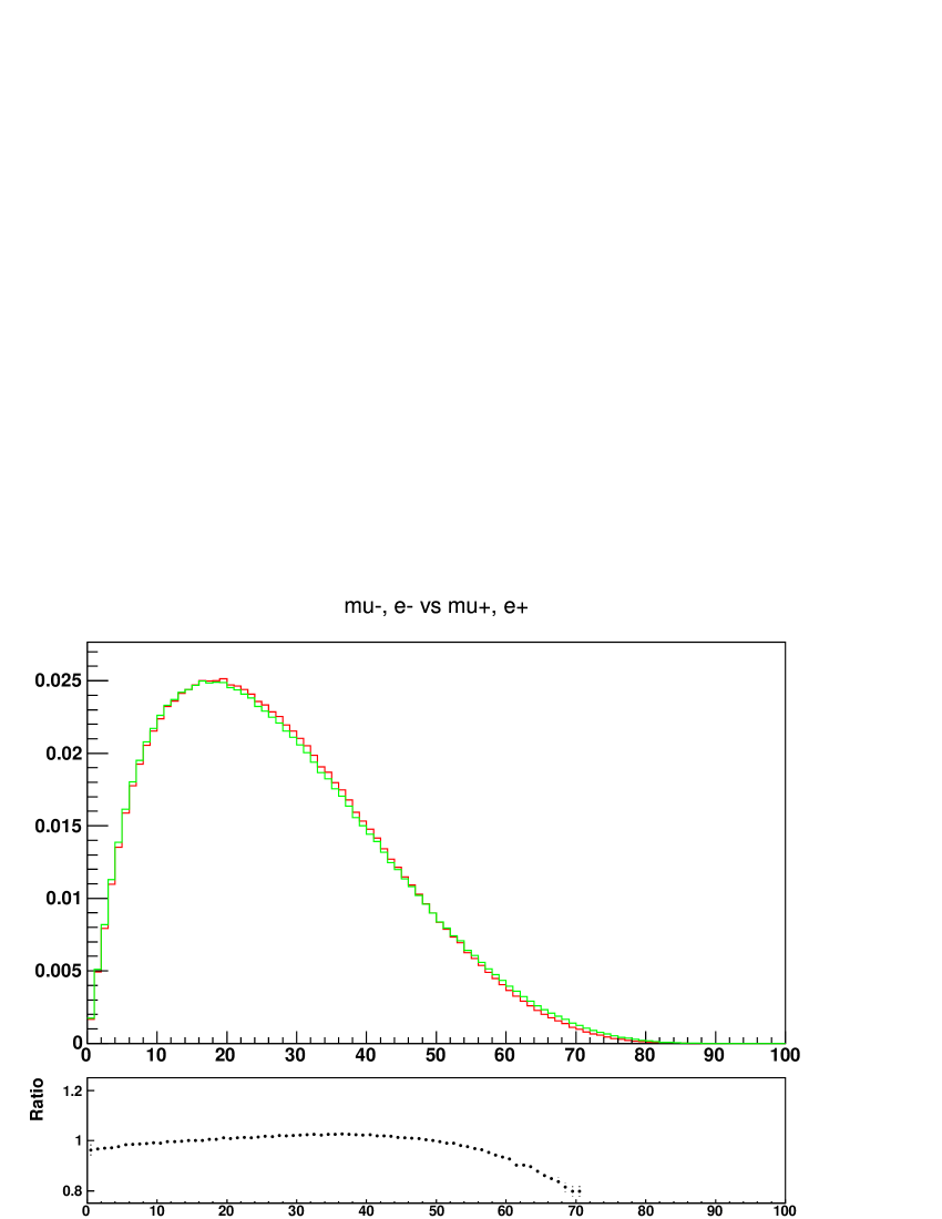
Figure B.1: Fractions of $\tau^{+}$ and $\tau^{-}$ energies carried by their visible decay products: two dimensional lego plots and one dimensional spectra¹⁸. Red line (and left scattergram) is sample with spin effects like of Higgs, green line (and right scattergram) is for modified sample after removing polarisation using TauSpinner weights, black line is ratio original/modified with whenever available superimposed result for the fitted functions.

B.2 The energy spectrum: $\tau^{-}\to\mu^{-},e^{-}$ vs $\tau^{+}\to\pi^{+}$

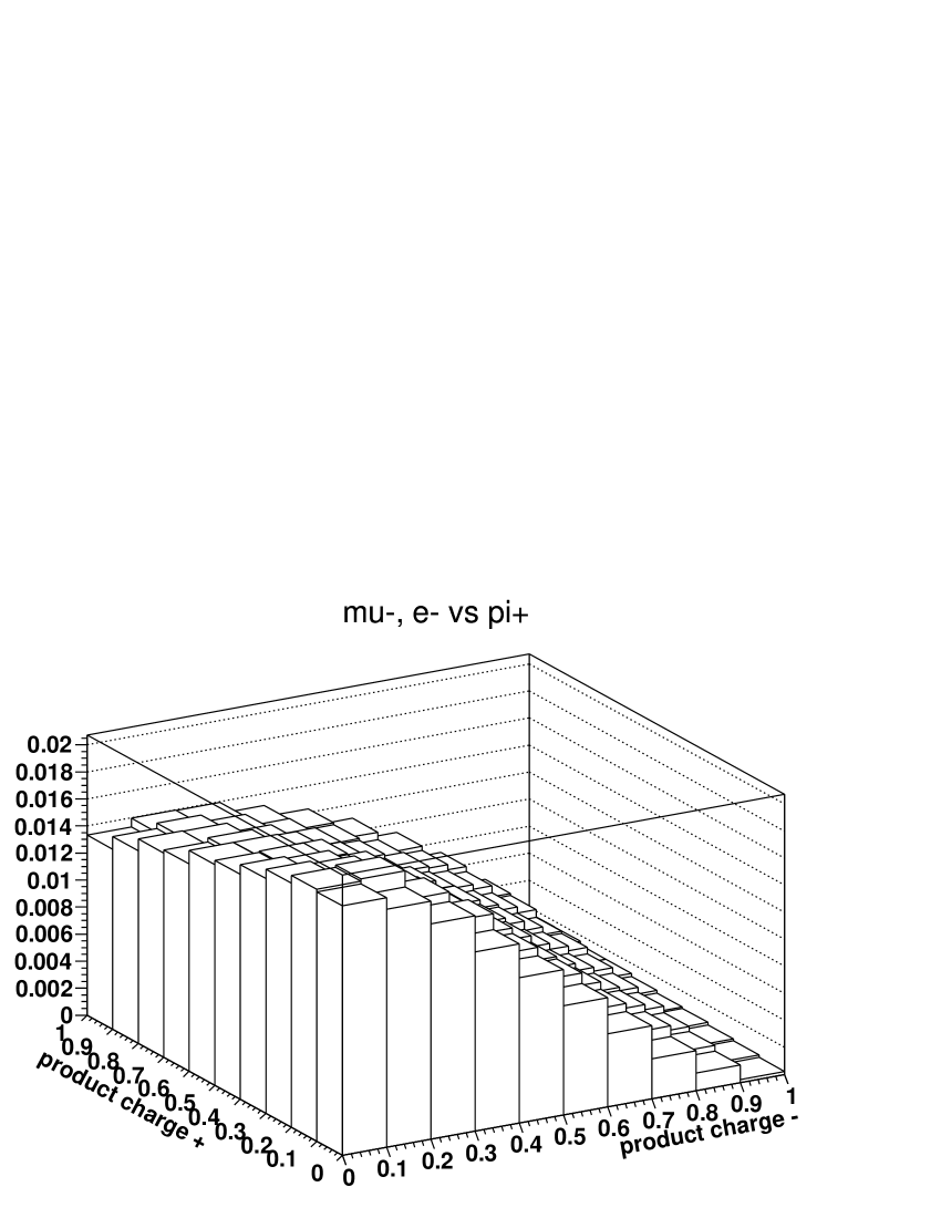
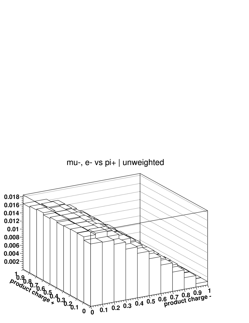
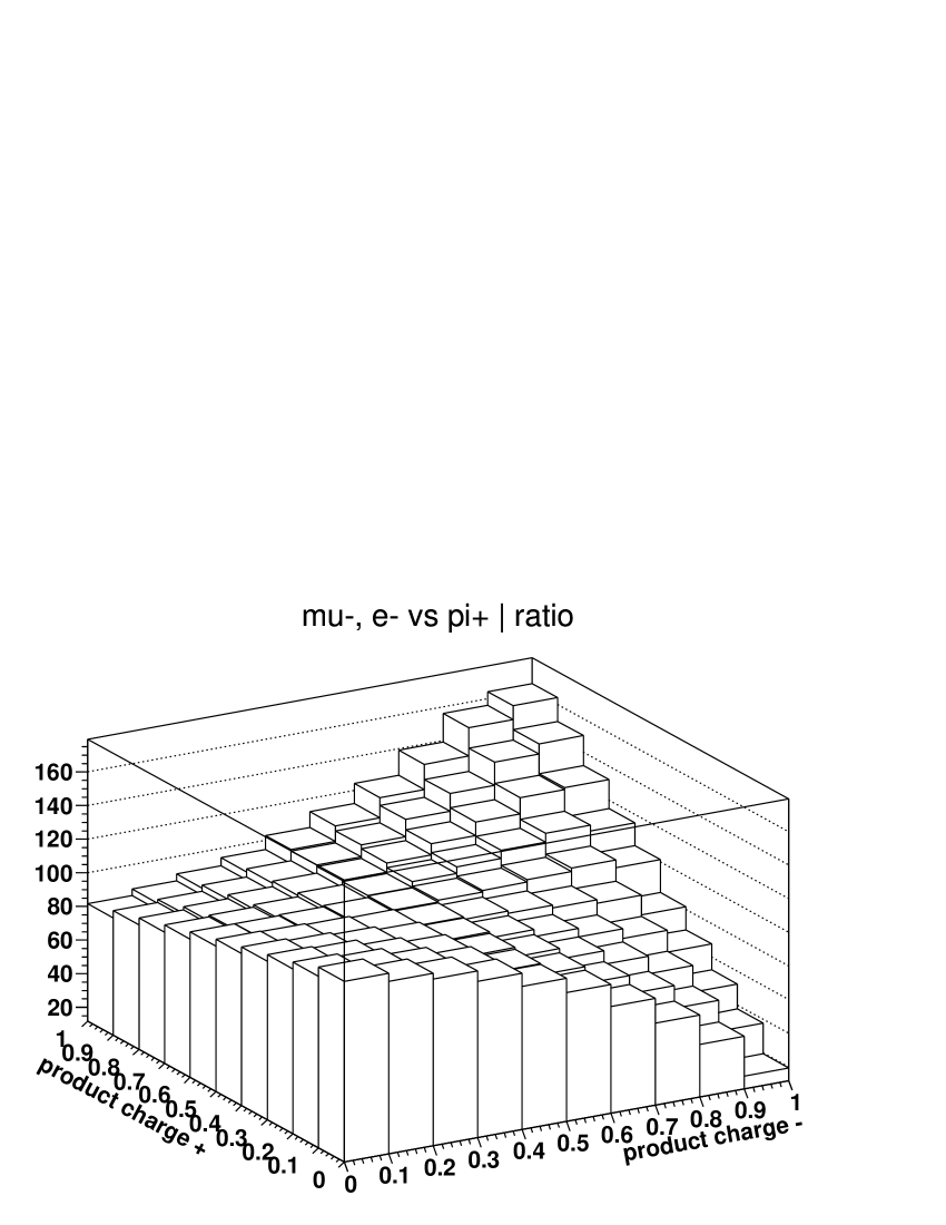
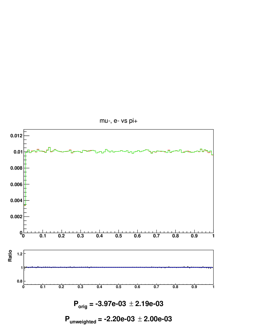
Figure B.2: Fractions of $\tau^{+}$ and $\tau^{-}$ energies carried by their visible decay products: two dimensional lego plots and one dimensional spectra¹⁸. Red line (and left scattergram) is sample with spin effects like of Higgs, green line (and right scattergram) is for modified sample after removing polarisation using TauSpinner weights, black line is ratio original/modified with whenever available superimposed result for the fitted functions.

B.3 The energy spectrum: $\tau^{-}\to\pi^{-}$ vs $\tau^{+}\to\mu^{+},e^{+}$

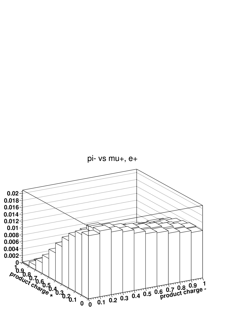
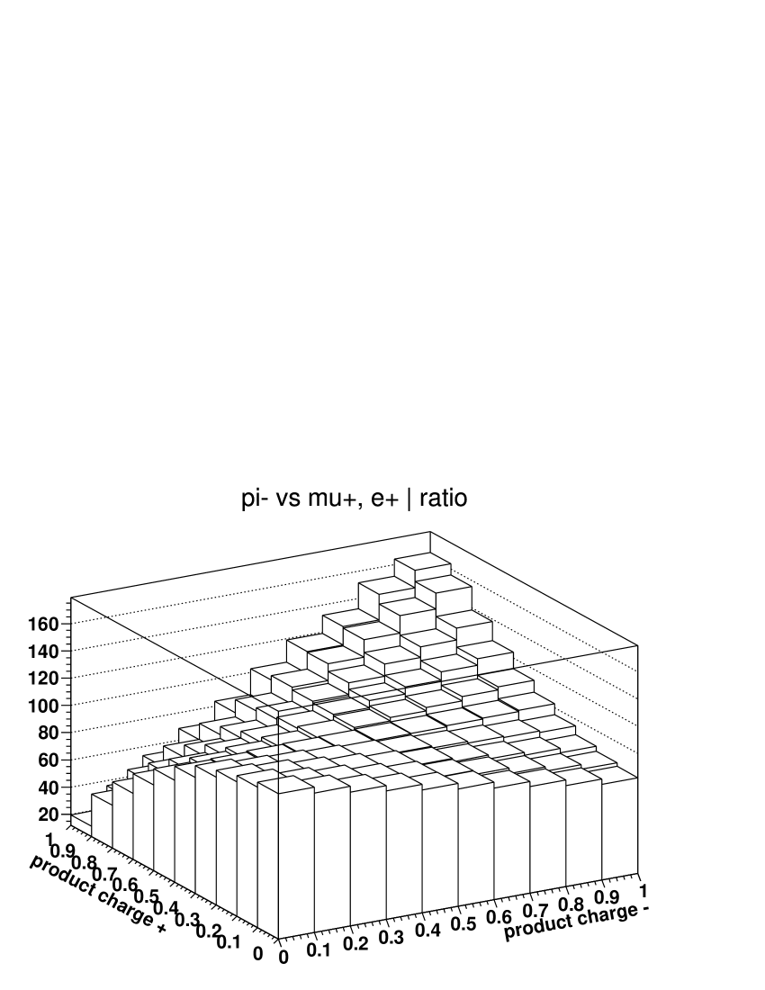
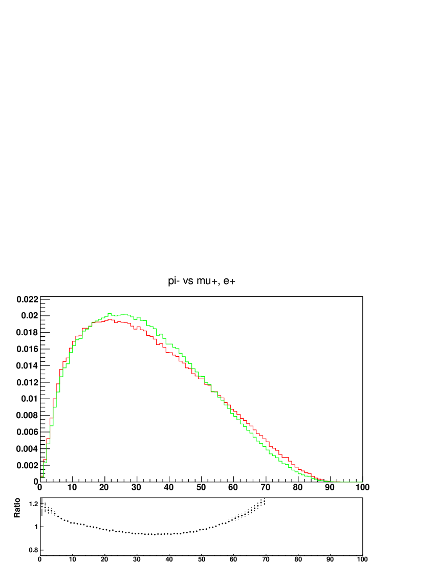
Figure B.3: Fractions of $\tau^{+}$ and $\tau^{-}$ energies carried by their visible decay products: two dimensional lego plots and one dimensional spectra¹⁸. Red line (and left scattergram) is sample with spin effects like of Higgs, green line (and right scattergram) is for modified sample after removing polarisation using TauSpinner weights, black line is ratio original/modified with whenever available superimposed result for the fitted functions.

B.4 The energy spectrum: $\tau^{-}\to\pi^{-}$ vs $\tau^{+}\to\pi^{+}$

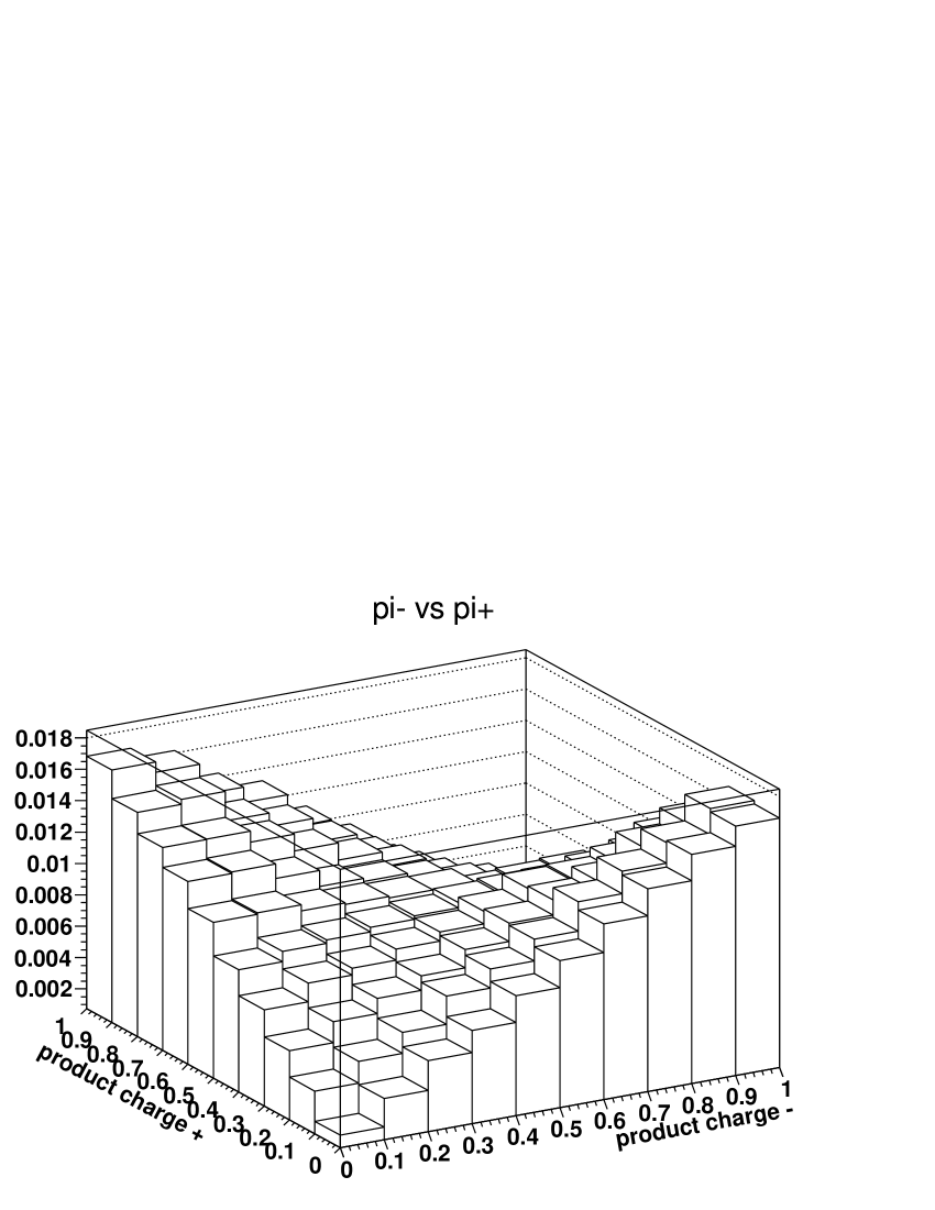
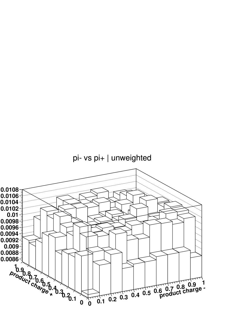
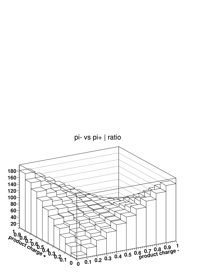
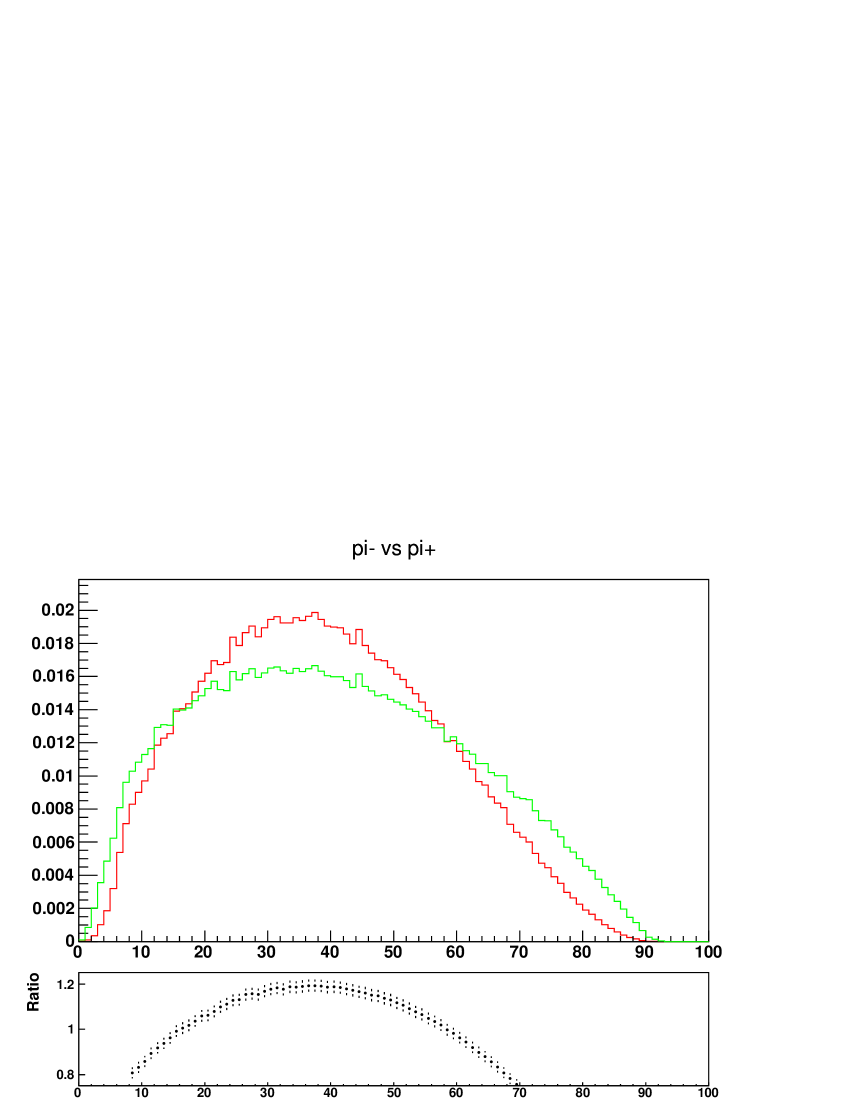
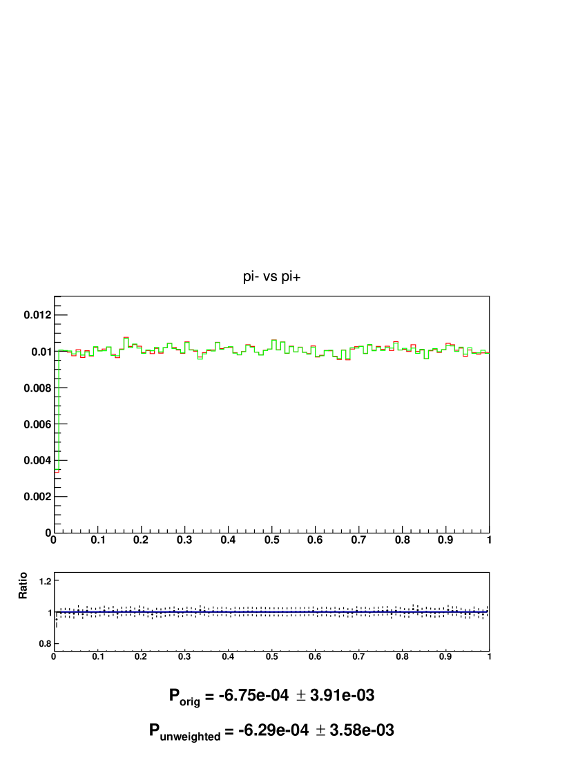
Figure B.4: Fractions of $\tau^{+}$ and $\tau^{-}$ energies carried by their visible decay products: two dimensional lego plots and one dimensional spectra¹⁸. Red line (and left scattergram) is sample with spin effects like of Higgs, green line (and right scattergram) is for modified sample after removing polarisation using TauSpinner weights, black line is ratio original/modified with whenever available superimposed result for the fitted functions.

B.5 The energy spectrum: $\tau^{-}\to\mu^{-},e^{-}$ vs $\tau^{+}\to\rho^{+}$

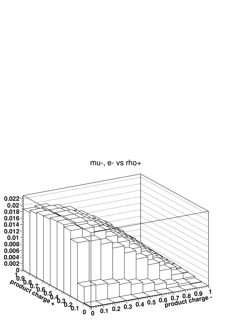
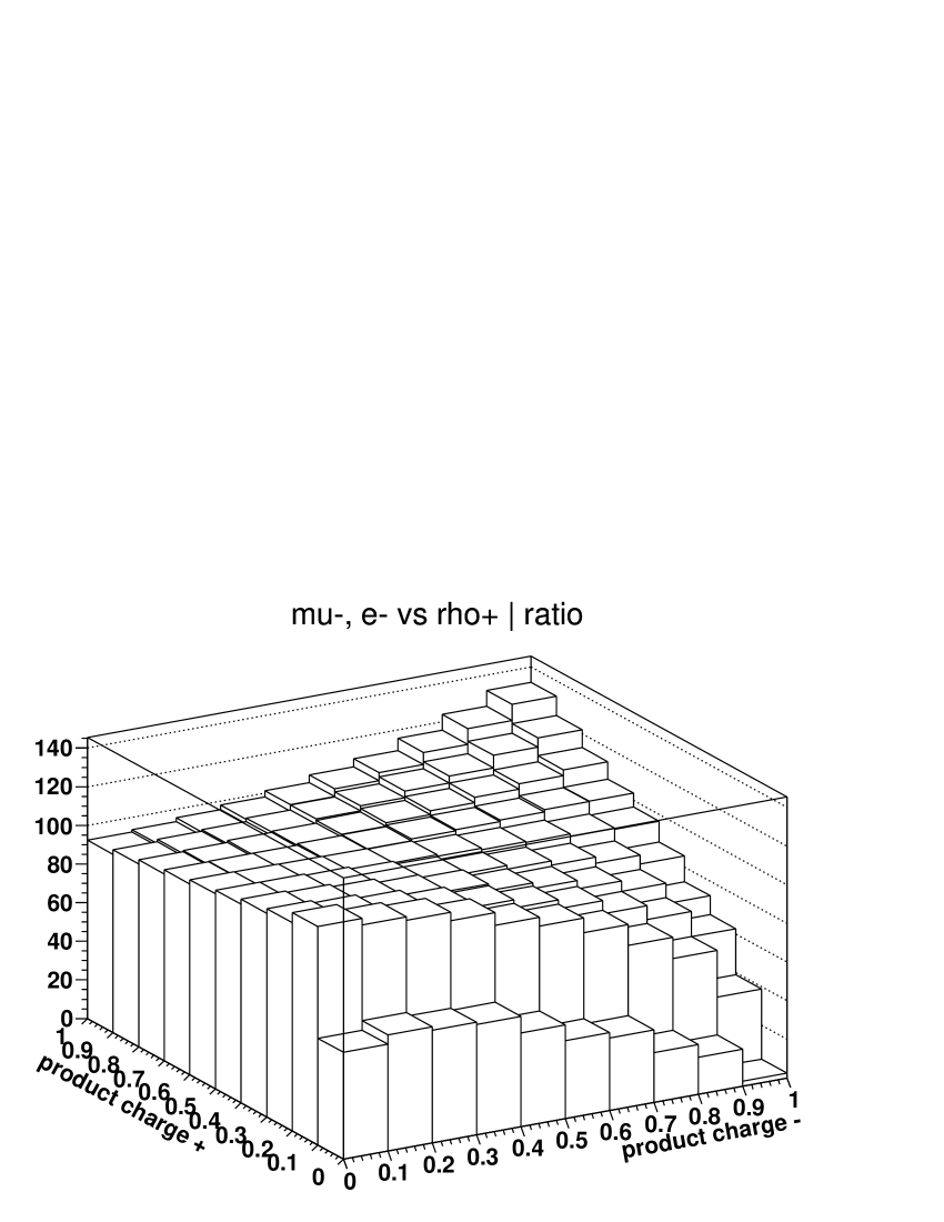
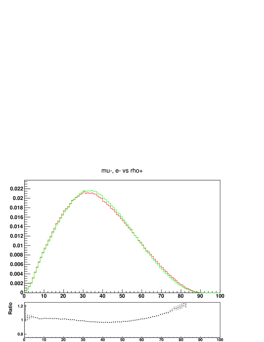
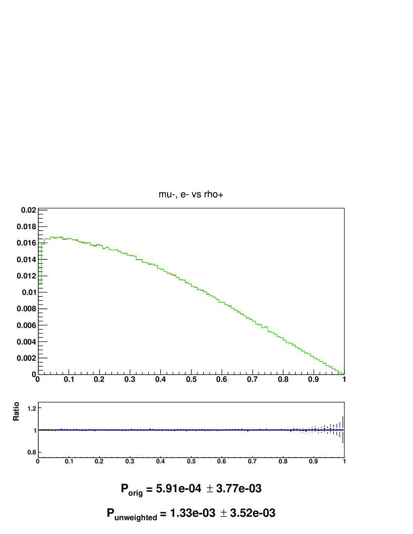
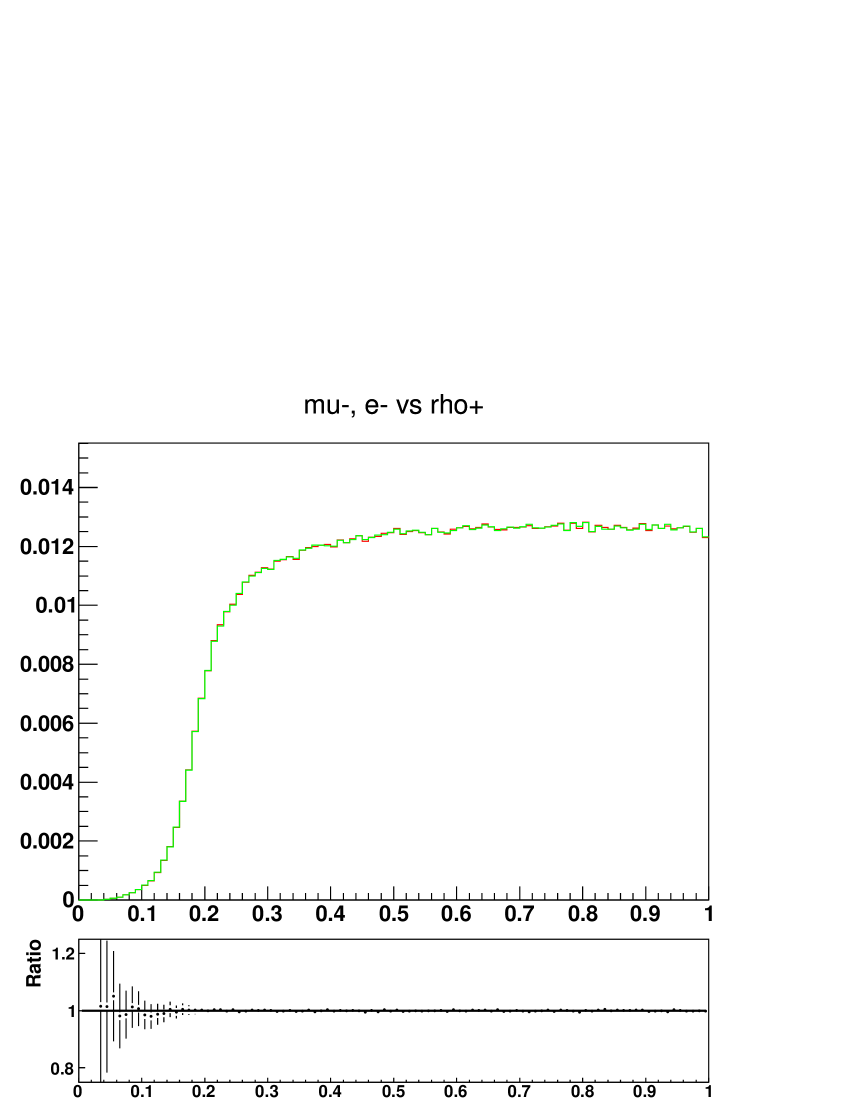
Figure B.5: Fractions of $\tau^{+}$ and $\tau^{-}$ energies carried by their visible decay products: two dimensional lego plots and one dimensional spectra¹⁸. Red line (and left scattergram) is sample with spin effects like of Higgs, green line (and right scattergram) is for modified sample after removing polarisation using TauSpinner weights, black line is ratio original/modified with whenever available superimposed result for the fitted functions.

B.6 The energy spectrum: $\tau^{-}\to\rho^{-}$ vs $\tau^{+}\to\mu^{+},e^{+}$

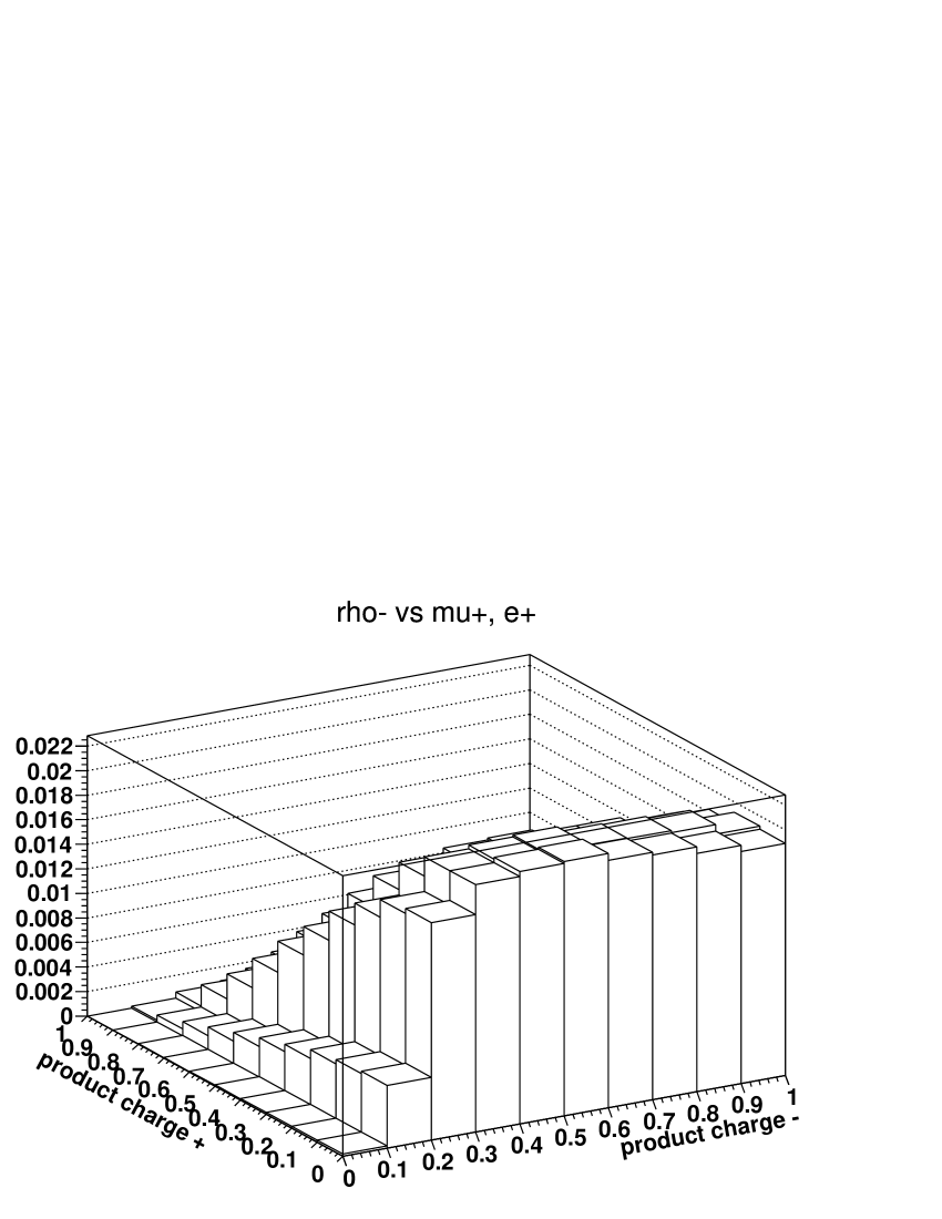
Figure B.6: Fractions of $\tau^{+}$ and $\tau^{-}$ energies carried by their visible decay products: two dimensional lego plots and one dimensional spectra¹⁸. Red line (and left scattergram) is sample with spin effects like of Higgs, green line (and right scattergram) is for modified sample after removing polarisation using TauSpinner weights, black line is ratio original/modified with whenever available superimposed result for the fitted functions.

B.7 The energy spectrum: $\tau^{-}\to\pi^{-}$ vs $\tau^{+}\to\rho^{+}$

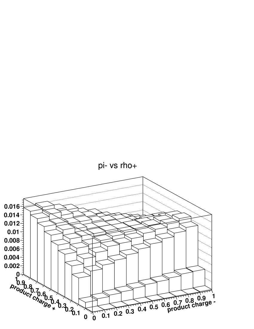
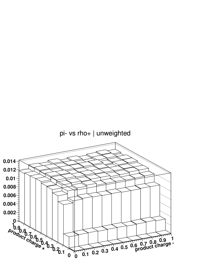
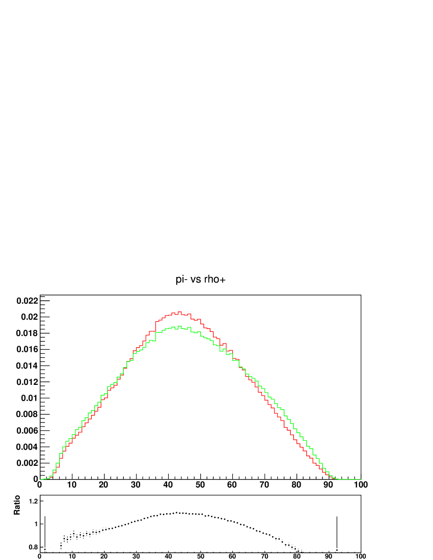
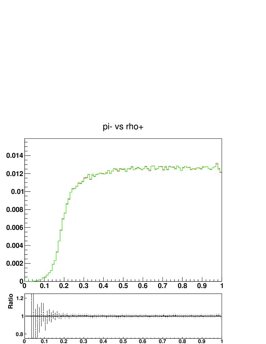
Figure B.7: Fractions of $\tau^{+}$ and $\tau^{-}$ energies carried by their visible decay products: two dimensional lego plots and one dimensional spectra¹⁸. Red line (and left scattergram) is sample with spin effects like of Higgs, green line (and right scattergram) is for modified sample after removing polarisation using TauSpinner weights, black line is ratio original/modified with whenever available superimposed result for the fitted functions.

B.8 The energy spectrum: $\tau^{-}\to\rho^{-}$ vs $\tau^{+}\to\pi^{+}$

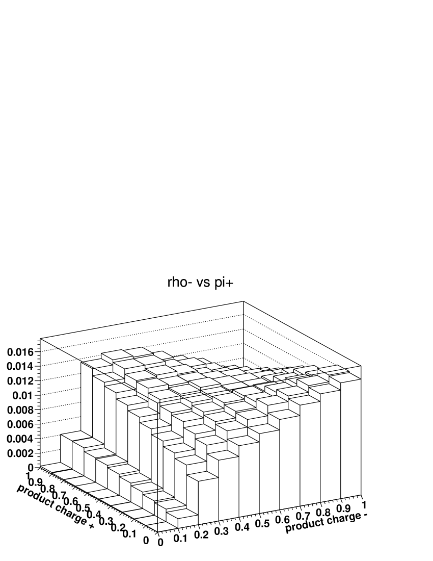
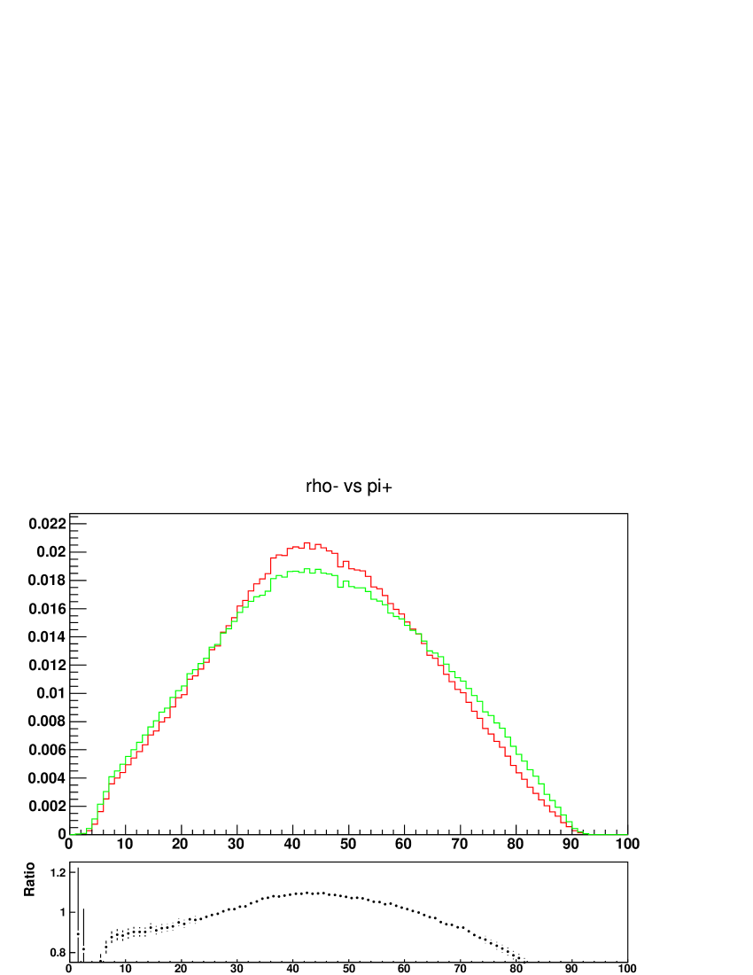
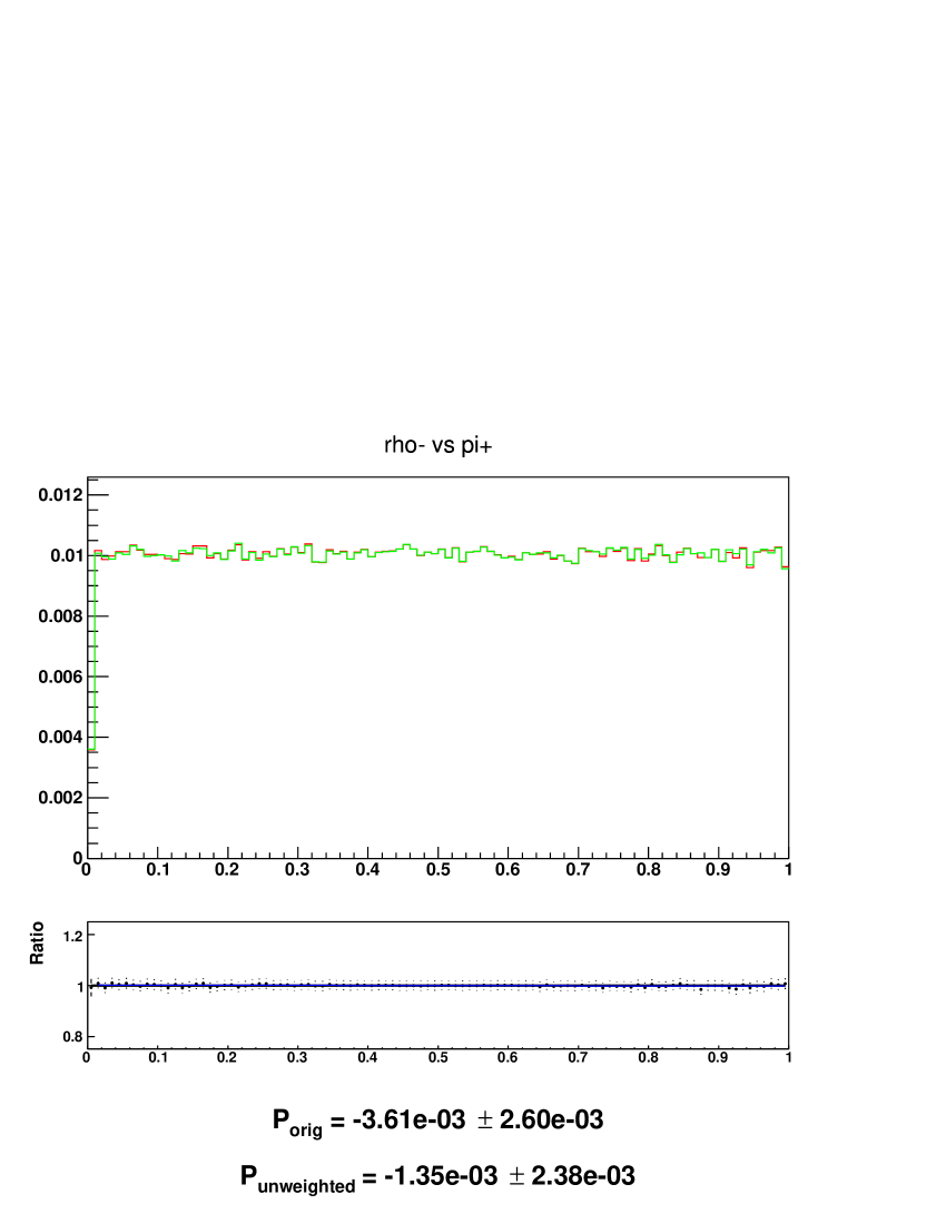
Figure B.8: Fractions of $\tau^{+}$ and $\tau^{-}$ energies carried by their visible decay products: two dimensional lego plots and one dimensional spectra¹⁸. Red line (and left scattergram) is sample with spin effects like of Higgs, green line (and right scattergram) is for modified sample after removing polarisation using TauSpinner weights, black line is ratio original/modified with whenever available superimposed result for the fitted functions.

B.9 The energy spectrum: $\tau^{-}\to\rho^{-}$ vs $\tau^{+}\to\rho^{+}$

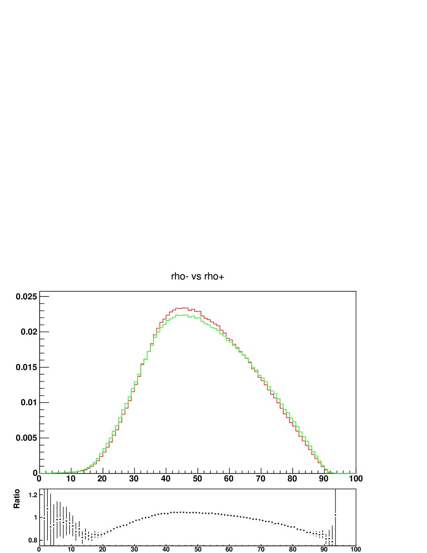
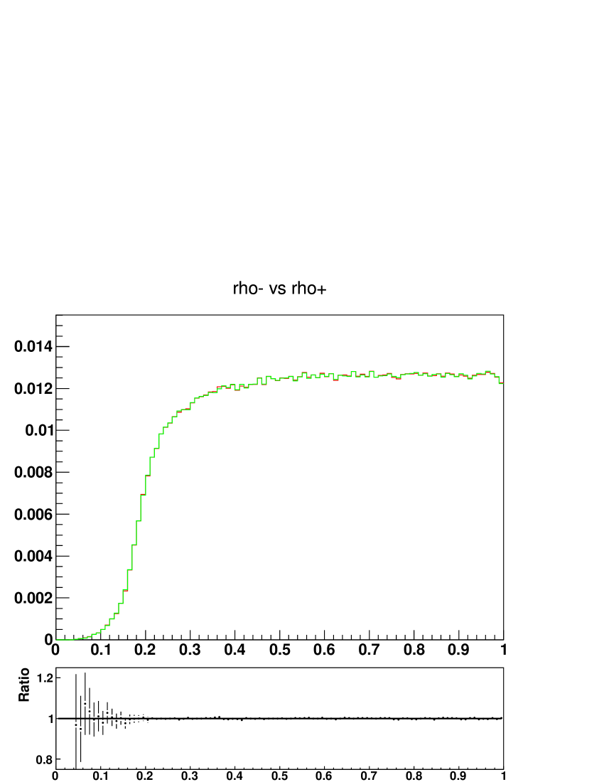
Figure B.9: Fractions of $\tau^{+}$ and $\tau^{-}$ energies carried by their visible decay products: two dimensional lego plots and one dimensional spectra. Red line (and left scattergram) is sample with spin effects like of Higgs, green line (and right scattergram) is for modified sample after removing polarisation using TauSpinner weights, black line is ratio original/modified.

References

- [1] ATLAS Collaboration, 0901.0512.
- [2] CMS Collaboration, JINST 3 (2008) S08004.
- [3] LHCb Collaboration, JINST 3 (2008) S08005.
- [4] ATLAS Collaboration, Eur.Phys.J. C72 (2012) 2062, 1204.6720.
- [5] I. Deigaard, CERN-THESIS-2012-091.
- [6] J. L. Harton, Nucl. Phys. Proc. Suppl. 40 (1995) 463–473.
- [7] ALEPH Collaboration, A. Heister et al., Eur. Phys. J. C20 (2001) 401–430, hep-ex/0104038.
- [8] Z. Czyczula, T. Przedzinski, and Z. Was, Eur.Phys.J. C72 (2012) 1988, 1201.0117.
- [9] S. Banerjee, J. Kalinowski, W. Kotlarski, T. Przedzinski, and Z. Was, Eur.Phys.J. C73 (2013) 2313, 1212.2873.
- [10] S. Jadach and Z. Wa̧s, Acta Phys. Polon. B15 (1984) 1151, Erratum: B16 (1985) 483.
- [11] P. Eberhard, B. van Eijk, J. Fuster, S. Jadach, A. Lutz, et al., CERN-EP-89-129, C89-02-20.1, C89-05-08.2.
- [12] T. Pierzchala, E. Richter-Was, Z. Was, and M. Worek, Acta Phys.Polon. B32 (2001) 1277–1296, hep-ph/0101311.
- [13] ATLAS Collaboration, ATLAS-CONF-2012-160.
- [14] N. Davidson, G. Nanava, T. Przedzinski, E. Richter-Was, and Z. Was, Comput.Phys.Commun. 183 (2012) 821–843, 1002.0543.
- [15] S. Jadach, Z. Wa̧s, R. Decker, and J. H. Kühn, Comput. Phys. Commun. 76 (1993) 361.
- [16] T. Sjostrand, S. Mrenna, and P. Skands, Comput. Phys. Commun. 178 (2008) 852–867, 0710.3820.
- [17] M. Dobbs and J. B. Hansen, Comput. Phys. Commun. 134 (2001) 41–46, https://savannah.cern.ch/projects/hepmc/.
- [18] N. Davidson, T. Przedzinski, and Z. Was, 1011.0937.
- [19] G. Altarelli, R. Kleiss, and C. Verzegnassi, CERN-89-08, CERN-89-08-V-1.
- [20] G. Altarelli, R. Kleiss, and C. Verzegnassi, CERN-89-08, CERN-89-08-V-3.
- [21] http://root.cern.ch/root/Availability.html .
- [22] A. van Hameren and Z. Was, Eur.Phys.J. C61 (2009) 33–49, 0802.2182.
- [23] E. Mirkes, Nucl.Phys. B387 (1992) 3–85.
- [24] E. Mirkes and J. Ohnemus, Phys.Rev. D50 (1994) 5692–5703, hep-ph/9406381.
- [25] CDF Collaboration Collaboration, T. Aaltonen et al., Phys.Rev. D88 (2013) 072002, 1307.0770.
- [26] R. Kleiss, Nucl. Phys. B347 (1990) 67–85.
- [27] Z. Was and S. Jadach, Phys. Rev. D41 (1990) 1425.
- [28] N. Davidson, G. Nanava, T. Przedzinski, E. Richter-Was, and Z. Was, TAUOLA and TAUOLA C++ Interface source code and documentation aviable from http://wasm.web.cern.ch/wasm/C++.html or http://tauolapp.web.cern.ch.
- [29] S. Jadach, B. Ward, and Z. Was, Comput.Phys.Commun. 130 (2000) 260–325, hep-ph/9912214.