Probabilistic Interpretation of Linear Solvers

Abstract

This manuscript proposes a probabilistic framework for algorithms that iteratively solve unconstrained linear problems $Bx=b$ with positive definite $B$ for $x$. The goal is to replace the point estimates returned by existing methods with a Gaussian posterior belief over the elements of the inverse of $B$, which can be used to estimate errors. Recent probabilistic interpretations of the secant family of quasi-Newton optimization algorithms are extended. Combined with properties of the conjugate gradient algorithm, this leads to uncertainty-calibrated methods with very limited cost overhead over conjugate gradients, a self-contained novel interpretation of the quasi-Newton and conjugate gradient algorithms, and a foundation for new nonlinear optimization methods.

1 Introduction

1.1 Motivation

Solving the unconstrained linear problem of finding $x$ in

(1) $$Bx=b\qquad\text{with symmetric, positive definite $B\in\mathbb{R}^{N\times N}$ and $b\in\mathbb{R}^{N}$}$$

is a basic task for computational linear algebra. It is equivalent to minimizing the quadratic $f(x)=\nicefrac{{1}}{{2}}x^{\intercal}Bx-x^{\intercal}b$, with gradient $F(x)=\nabla_{x}f(x)=Bx-b$ and constant Hessian $B$. If $N$ is too large for exact solution, iterative solvers such as the method of conjugate gradients [27] (CG) are widely applied. These methods produce a sequence of estimates $\{x_{i}\}_{i=0,\dots,M}$, updated by evaluating $F(x_{i})$. The question addressed here is: Assume we run an iterative solver for $M<N$ steps. How much information does doing so provide about $B$ and its (pseudo-) inverse $H$? If we had to give estimates for $B$, $H$, and for the solution to related problems $B\tilde{x}=\tilde{b}$, what should they be, and how big of an ‘error bar’ (a joint posterior distribution) should we put on these estimates? The gradient $F(x_{i})$ provides an error residual on $x_{i}$, but not on $B,H$ and $\tilde{x}$.

It will turn out that a family of quasi-Newton methods (§1.2), more widely used to solve nonlinear optimization problems, can help answer this question, because classic derivations of these methods can be re-formulated and extended into a probabilistic interpretation of these methods as maxima of Gaussian posterior probability distributions (§2). The covariance of these Gaussians offers a new object of interest and provides error estimates (§3). Because there are entire linear spaces of Gaussian distributions with the same posterior mean but differing posterior error estimates, selecting one error measure consistent with the algorithm is a new statistical estimation task (§4).

1.2 The Dennis family of secant methods

The family of secant update rules for an approximation to the Newton-Raphson search direction is among the most popular building blocks for continuous nonlinear programming. Their evolution chiefly occurred from the late 1950s [8] to the 1970s, and is widely understood to be crowned by the development of the BFGS rule due to Broyden [5], Fletcher [18], Goldfarb [22] and Shanno [39], which now forms a core part of many contemporary optimization methods. But the family also includes the earlier and somewhat less popular DFP rule of Davidon [8], Fletcher and Powell [19]; the Greenstadt [23] rule, and the so-called symmetric rank-1 method [8, 4]. Several authors have proposed grouping these methods into broader classes, among them Broyden in 1967 [4] (subsequently refined by Fletcher [18]) and Davidon in 1975 [9]. Of particular interest here will be a class of updates formulated in 1971 by Dennis [10], which includes all the specific rules cited above. It is the class of update rules mapping a current estimate $B_{0}$ for the Hessian, a vector-valued pair of observations $y_{i}=F(x_{i})-F(x_{i-1})\in\mathbb{R}^{N}$ and $s_{i}=x_{i}-x_{i-1}$ with $y_{i}=Bs_{i}$, into a new estimate $B_{i}$ of the form

(2) $$B_{i+1}=B_{i}+\frac{(y_{i}-B_{i}s_{i})c_{i}^{\intercal}+c_{i}(y_{i}-B_{i}s_{i})^{\intercal}}{c_{i}^{\intercal}s_{i}}-\frac{c_{i}s_{i}^{\intercal}(y_{i}-B_{i}s_{i})c_{i}^{\intercal}}{(c_{i}^{\intercal}s_{i})^{2}}\qquad\text{for some }c_{i}\in\mathbb{R}^{N}.$$

This ensures the secant relation $y_{i}=B_{i+1}s_{i}$, sometimes called ‘the quasi-Newton Equation’ [13]. Convergence of the sequence of iterates $x_{i}$ for various members of this class (and the classes of Broyden and Davidon) are well-understood [21, 12]. The rules named above can be found in the Dennis class as [37]:

(3) Symmetric Rank-1 (SR1) $$c =y-B_{0}s$$

(4) Powell Symmetric Broyden [36] $$c =s$$

(5) Greenstadt [23] $$c =B_{0}s$$

(6) Davidon Fletcher Powell (DFP) $$c =y$$

(7) Broyden Fletcher Goldfarb Shanno (BFGS) $$c =y+\sqrt{\frac{y^{\intercal}s}{s^{\intercal}B_{0}s}}B_{0}s$$

Inverse updates

Because the update of Equation (2) is of rank 2, the corresponding estimate for the inverse $H=B^{-1}$ (assuming it exists) can be constructed using the matrix inversion lemma. Alternatively, all Dennis rules can also be used as inverse updates [13], i.e. estimates for $H$ itself, by exchanging $s\operatorname*{\leftrightarrowtriangle}y$ and $B\operatorname*{\leftrightarrowtriangle}H$, $B_{0}\operatorname*{\leftrightarrowtriangle}H_{0}$ above (corresponding to the secant relation $s=Hy$). Interestingly, the DFP and BFGS updates are duals of each other under this exchange [13]: The inverse of $B_{1}$ as constructed by the DFP rule (6) equals the $H_{1}$ arising from the inverse BFGS rule (7). This does not mean BFGS and DFP are the same, but only that they fill opposing roles in the inverse and direct formulation. To avoid confusion, in this text the DFP rule will always be used in the sense of a direct update (estimating $B$, with $c=y$), and the BFGS rule in the inverse sense (i.e. estimating $H$, with $c=s$). The first parts of this text will focus on direct updates and thus mostly talk about the DFP method instead of the BFGS rule. All results extend to the inverse models (and thus BFGS) under the exchange of variables mentioned above. Sections 3.2 and 4 will make some specific choices geared to inverse updates. They will then talk explicitly about BFGS, always in the sense of an inverse update.

Towards probabilistic quasi-Newton methods

This text gives a probabilistic interpretation of the Dennis family, for the linear problems of Eq. (1). We will interpret the secant methods as estimators of (inverse) Hessians of an objective function, and ask what kind of prior assumptions would give rise to these specific estimators. This results in a self-contained derivation of inference rules for symmetric matrices. Some of the rules quoted above can be motivated as ‘natural’ from the inference perspective.

Another major strand of nonlinear optimization methods extends from the conjugate gradient algorithm of Hestenes & Stiefel [27] for linear problems, nonlinearly extended by Fletcher and Reeves [20] and others. On linear problems, the CG and quasi-Newton ideas are closely linked: Nazareth [32] showed that CG is equivalent to BFGS for linear problems (with exact line searches, when the initial estimate $B_{0}=\boldsymbol{I}$). More generally, Dixon [16, 17] showed for quasi-Newton methods in the Broyden class (which also contains the methods listed above) that, under exact line searches and the same starting point, all methods in Broyden’s class generate a sequence of points identical to CG, if the starting matrix $B_{0}$ is taken as a preconditioner of CG. In this sense, this text also provides a novel derivation for conjugate gradients, and will use several well-known properties of that method. Implications of the results presented herein to nonlinear variants of conjugate gradients will be left for future work.

1.3 Numerical methods perform inference — The value of a statistical interpretation

The defining aspect of quasi-Newton methods is that they approximate—estimate—the Hessian matrix of the objective function, or its inverse, based on evaluations—observations—of the objective’s gradient and certain prior structural restrictions on the estimate. They can therefore be interpreted as inferring the latent quantity $B$ or $H$ from the observed quantities $s,y$. This creates a connection to statistics and probability theory, in particular the probabilistic framework of encoding prior assumptions in a probability measure over a hypothesis space, and describing observations using a likelihood function, which combines with the prior according to Bayes’ theorem into a posterior measure over the hypothesis space (§2).

On the one hand, this elucidates prior assumptions of quasi-Newton methods (§3). On the other, it suggests new functionality for the existing methods, in particular error estimates on $B$ and $H$ (§4). In future work, it may also allow for algorithms robust to ‘noisy’ linear maps, such as they arise in physical inverse problems.

The interpretation of numerical problems as estimation was pointed out by statisticians like Diaconis in 1988 [14], and O’Hagan in 1992 [35], well after the introduction of quasi-Newton methods. To the author’s knowledge, the idea has rarely attracted interest in numerical mathematics, and has not been studied in the context of quasi-Newton methods before recent work by Hennig & Kiefel [25, 26]. An argument sometimes raised against analysing numerical methods probabilistically is that numerical problems do not generally feature an aspect of randomness. But probability theory makes no formal distinction between epistemic uncertainty, arising from lack of knowledge, and aleatoric uncertainty, arising from ‘randomness’, whatever the latter may be taken to mean precisely. Randomness is not a prerequisite for the use of probabilities. Those who do feel uneasy about applying probability theory to unknown deterministic quantities, however, may prefer another, perhaps more subjective argument: From the point of view of a numerical algorithm’s designer, the ‘population’ of problems that practitioners will apply the algorithm to does in fact form a probability distribution from which tasks are ‘sampled’.

Numerical algorithms running on a finite computational budget make numerical errors. A notion of the imprecision of this answers is helpful, in particular when the method is used within a larger computational framework. Explicit error estimates can be propagated through the computational pipeline, helping identify points of instability, and to distribute or save computational resources. Needless to say, it makes no sense to ask for the exact error (if the exact difference between the true and estimated answer where known, the exact answer would be known, too). But it is meaningful to ask for the remaining volume of hypotheses consistent with the computations so far. This paper attempts to construct such an answer for linear problems.

1.4 Overview of main results

As pointed out above, although quasi-Newton methods are most popular for nonlinear optimization, here the focus will be on linear problems. Extending the probabilistic interpretation constructed here to the nonlinear setting of inferring the (inverse) Hessian of a function $f$ will be left for future work (see [26] for pointers). The present aim is an iterative linear solver iterating through posterior beliefs $\{p_{t}(x,H)\}_{t=1,\dots,M}$ for $H=B^{-1}$ and the solution $x=Hb$ of the linear problem. These beliefs will be constructed as Gaussian densities $p_{t}(H)=\mathcal{N}(H;H_{t},V_{t})$ over the elements of $H$, with mean $H_{t}$ and covariance matrix $V_{t}$.

The results in this paper significantly clarify and extend previous results by Hennig & Kiefel [26] and Hennig [24]. Here is a brief outlook of the main results:

Dennis family derived in a symmetric hypothesis class (§2)

As a probabilistic interpretation of results by Dennis & Moré [13] and Dennis & Schnabel [11], Hennig [24] provided a derivation of rank-2 secant methods in terms of two independent observations of two separate parts of the Hessian. This viewpoint affords a nonparametric extension to nonlinear optimization, but is not particularly elegant. This paper provides a cleaner derivation: the Dennis family can in fact be derived naturally from a prior over only symmetric matrices. This extends the results of Dennis & Schnabel [11], from statements about the maximum of a Frobenius norm in the space of symmetric matrices to the entire structure of that norm in that space.

New interpretation for SR1, Greenstadt, DFP & BFGS updates (§3)

The choice of prior parameters distinguishes between the members of the Dennis family. An analysis shows that DFP and BFGS are ‘more correct’ than other members of the family in the sense that they are consistent with exact probabilistic inference for the entire run of the algorithm, while general Dennis rules are only consistent after the first step (Lemmas 6 and 7). Further, SR1, Greenstadt, DFP and BFGS all use different prior measures that, although all ‘scale-free’, give imperfect notions of calibration for the prior measure. Finally, because BFGS is equivalent to CG ([32] and Lemma 8), its set of evaluated gradients is orthogonal. This allows a computationally convenient parameterization of posterior uncertainty. Overall, the picture arising is that, from the probabilistic perspective, the DFP and particularly BFGS methods have convenient numerical properties, but their posterior measure can be calibrated better.

Posterior uncertainty by parameter estimation (§4)

It will transpire that the decision for a specific member of the Dennis family still leaves a space of possible choices of prior covariances consistent with this update rule. Constructing a meaningful posterior uncertainty estimate (covariance) on $H$ after finitely many steps requires a choice in this unidentified space, which, as in other estimation problems, needs to be motivated based on some notion of regularity in $H$. Several possible choices are discussed in Section 3, all of which add very low overhead to the standard conjugate gradient algorithm.

2 Gaussian inference from matrix-vector multiplications

2.1 Introduction to Gaussian inference

Gaussian inference—probabilistic inference using both a Gaussian prior and a Gaussian likelihood—is one of the best-studied areas of probabilistic inference. The following is a very brief introduction; more can be found in introductory texts [38, 29]. Consider a hypothesis class consisting of elements of the $D$-dimensional real vector space, $v\in\mathbb{R}^{D}$, and assign a Gaussian prior probability density over this space:

(8) $$p(v)=\mathcal{N}(v;\mu,\Sigma)\colonequals\frac{1}{(2\pi)^{D/2}|\Sigma|^{1/2}}\exp\left(-\frac{1}{2}(v-\mu)^{\intercal}\Sigma^{-1}(v-\mu)\right),$$

parametrised by mean vector $\mu\in\mathbb{R}^{D}$ and positive definite covariance matrix $\Sigma\in\mathbb{R}^{D\times D}$. If we now observe a linear mapping $A^{\intercal}v+a=y\in\mathbb{R}^{M}$ of $v$, up to Gaussian uncertainty of covariance $\Lambda\in\mathbb{R}^{M\times M}$, i.e. according to the likelihood function

(9) $$p(y\,|\,A,a,v)=\mathcal{N}(y;A^{\intercal}v+a,\Lambda),$$

then, by Bayes’ theorem and a simple linear computation (see e.g. [38, §2.1.2]), the posterior, the unique distribution over $v$ consistent with both prior and likelihood, is

(10) $$p(v\,|\,y,A,a)=\mathcal{N}[v;\mu+\Sigma A(A^{\intercal}\Sigma A+\Lambda)^{-1}(y-A^{\intercal}\mu-a),\Sigma-\Sigma A(A^{\intercal}\Sigma A+\Lambda)^{-1}A^{\intercal}\Sigma].$$

This derivation also works in the limit of perfect information, i.e. for a well-defined limit of $\Lambda\operatorname*{\rightarrowtriangle}0$, in which case the likelihood converges to the Dirac distribution $p(y\,|\,A,a,v)\operatorname*{\rightarrowtriangle}\delta(y-A^{\intercal}v-a)$. The crucial point is that constructing the posterior after linear observations involves only linear algebraic operations, with the posterior covariance (the ‘error bar’) using many of the computations also required to compute the mean (the ‘best guess’).

Gaussian inference is closely linked to least-squares estimation: Because the logarithm is concave, the maximum of the posterior (10) (which equals the mean) is also the minimizer of the quadratic norm (using $\|x\|_{K}^{2}\colonequals x^{\intercal}K^{-1}x.$)

(11) $$-2\log p(v\,|\,y,A,a)=\|y-A^{\intercal}v-a\|_{\Lambda}^{2}+\|v-\mu\|_{\Sigma}^{2}+\mathop{\operator@font const}\nolimits.$$

The added value of the probabilistic interpretation is embodied in the posterior covariance, which quantifies remaining degrees of freedom of the estimator, and can thus also be interpreted as a measure of uncertainty, or estimated error.

2.2 Inference on asymmetric matrices from matrix vector multiplications

We now consider Gaussian inference in the specific context of iterative solvers for linear problems as defined in Eq. (1). Our solver shall maintain a current probability density estimate, either $p_{i}(B)$ for $p_{i}(H)$, $i=0,\dots,M$. The solver does not have direct access to $B$ itself, but only to a function mapping $s\operatorname*{\rightarrowtriangle}Bs$, for arbitrary $s\in\mathbb{R}^{N}$.

It is possible to use the Gaussian inference framework in the context of secant methods [26] through the use of Kronecker algebra: We write the elements of $B$ as a vector $\overrightarrow{B}\in\mathbb{R}^{N^{2}}$, indexed as $\overrightarrow{B}_{ij}$ by the matrix’ index set $(i,j)\in\mathbb{R}\times\mathbb{R}$. The Kronecker product provides the link between such ‘vectorized matrices’ and linear operations (e.g. [40]). The Kronecker product $A\otimes C$ of two matrices $A\in\mathbb{R}^{M_{a}\times N}$ and $C\in\mathbb{R}^{M_{c}\times N}$ is the $M_{a}M_{c}\times N^{2}$ matrix with elements $(A\otimes C)_{(ij)(k\ell)}=A_{ik}C_{j\ell}$. It has the property $(A\otimes C)\overrightarrow{B}=\overrightarrow{ABC^{\intercal}}$. Thus, $\overrightarrow{BS}$ can be written as $(\boldsymbol{I}\otimes S)\overrightarrow{B}$, which allows incorporating the kind of observations made by an iterative solver in a Gaussian inference framework, according to the following Lemma.

Lemma 1 (proof in Hennig & Kiefel, 2013).

Given a Gaussian prior over a general quadratic matrix $\overrightarrow{B}$, with prior mean $\overrightarrow{B}_{0}$ and a prior covariance with Kronecker structure, $p(B)=\mathcal{N}(\overrightarrow{B};\overrightarrow{B}_{0},W\otimes W)$, the posterior mean after observing $BS=Y\in\mathbb{R}^{N\times M}$ (i.e. $M$ projections along the line-search directions $S\in\mathbb{R}^{N\times M}$) is

(12) $$B_{M}=B_{0}+(Y-B_{0}S)(S^{\intercal}WS)^{-1}WS^{\intercal},$$

and the posterior covariance is

(13) $$V_{M}=W\otimes\left[W-WS(S^{\intercal}WS)^{-1}WS^{\intercal}\right].$$

This implies, for example, that Broyden’s rank-1 method [3] is equal to the posterior mean update after a single line search for the parameter choice $W=\boldsymbol{I}$. This is a probabilistic re-phrasing of the much older observation, most likely by Dennis & Moré, [13], that Broyden’s method minimizes a change in the Frobenius norm $\|B_{i}-B_{i-1}\|_{F,\boldsymbol{I}}$ such that $B_{i}s_{i}=y_{i}$. The weighted Frobenius norm $\|A\|_{F,W}^{2}=\operatorname{tr}(AW^{-1}A^{\intercal}W^{-1})$ (with the positive definite weighting $W$) is the $\ell_{2}$ loss on vectorized matrices in the sense that $\|A\|_{F,W}^{2}=\|\overrightarrow{A}\|_{W\otimes W}^{2}$.

An important observation is that Broyden’s method ceases to be a direct match to this update after the first line search, because matrix $S^{\intercal}WS$ is not a diagonal matrix. This matrix will come to play a central role; we will call it the Gram matrix, because it is an inner product of $S$ weighted by the positive definite $W$.

2.2.1 Symmetric hypothesis classes

It is well known that, because the posterior mean of Eq. (12) is not in general a symmetric matrix, it is a suboptimal learning rule for the Hessian of an objective function. Which is why this class was quickly abandoned in favour of the rank-2 updates in the Dennis family mentioned above. Dennis & Moré [13] and Dennis & Schnabel [11] showed that the minimizer of weighted Frobenius regularizers (the maximizer of the Gaussian posterior) within the linear subspace of symmetric matrices is given by the Dennis class of update rules. Hennig & Kiefel [26] constructed a probabilistic interpretation based on this derivation, which involves doubling the input domain of the objective function and introducing two separate, independent observations. This has the advantage of allowing for relatively straightforward nonparametric extensions, and a broad class of noise models for cases in which gradients can not be evaluated without error [24]. But artificially doubling the input dimensionality is dissatisfying.

We now introduce a cleaner derivation of the same updates, by explicitly restricting the hypothesis class to symmetric matrices. This gives the covariance matrix a more involved structure than the Kronecker product, and makes derivations more challenging. It results in a new interpretation for the Dennis class, fully consistent with the probabilistic framework. Since the identity of the posterior mean was known from [13, 11] and [26], the interesting novel aspect here is the structure of the posterior covariance. In essence, it provides insight into the structure of the loss function around the previously known estimates.

We begin by building a Gaussian prior over the symmetric matrices, using the symmetrization operator $\Gamma$, the linear operator acting on vectorized matrices defined implicitly through its effect $\Gamma\overrightarrow{A}=\nicefrac{{1}}{{2}}\overrightarrow{(A+A^{\intercal})}$ (explicit definition in Appendix A.1).

Lemma 2 (proof in Appendix A.1).

Assuming a Gaussian prior $p(B)=\mathcal{N}(\overrightarrow{B};\overrightarrow{B}_{0},W\otimes W)$ over the space of square matrices $B\in\mathbb{R}^{N\times N}$ with Kronecker covariance $\operatorname{cov}(B_{ij},B_{k\ell})=W_{ik}W_{j\ell}$ (this requires $W$ to be a symmetric positive definite matrix), the prior over the symmetric matrix $\Gamma\overrightarrow{B}$ is $p(B)=\mathcal{N}(\Gamma\overrightarrow{B};\Gamma\overrightarrow{B}_{0},W\mathchoice{{\ooalign{$\displaystyle\otimes$\cr\hfil$\displaystyle\ominus$\hfil\cr}}}{{\ooalign{$\textstyle\otimes$\cr\hfil$\textstyle\ominus$\hfil\cr}}}{{\ooalign{$\scriptstyle\otimes$\cr\hfil$\scriptstyle\ominus$\hfil\cr}}}{{\ooalign{$\scriptscriptstyle\otimes$\cr\hfil$\scriptscriptstyle\ominus$\hfil\cr}}}W)$.

Here, $W\mathchoice{{\ooalign{$\displaystyle\otimes$\cr\hfil$\displaystyle\ominus$\hfil\cr}}}{{\ooalign{$\textstyle\otimes$\cr\hfil$\textstyle\ominus$\hfil\cr}}}{{\ooalign{$\scriptstyle\otimes$\cr\hfil$\scriptstyle\ominus$\hfil\cr}}}{{\ooalign{$\scriptscriptstyle\otimes$\cr\hfil$\scriptscriptstyle\ominus$\hfil\cr}}}W=\Gamma(W\otimes W)\Gamma^{\intercal}$ is the symmetric Kronecker product of $W$ with itself (see e.g. [40] for an earlier mention). It is the matrix containing elements

(14) $$(W\mathchoice{{\ooalign{$\displaystyle\otimes$\cr\hfil$\displaystyle\ominus$\hfil\cr}}}{{\ooalign{$\textstyle\otimes$\cr\hfil$\textstyle\ominus$\hfil\cr}}}{{\ooalign{$\scriptstyle\otimes$\cr\hfil$\scriptstyle\ominus$\hfil\cr}}}{{\ooalign{$\scriptscriptstyle\otimes$\cr\hfil$\scriptscriptstyle\ominus$\hfil\cr}}}W)_{ij,k\ell}=\nicefrac{{1}}{{2}}(W_{ik}W_{j\ell}+W_{jk}W_{i\ell}).$$

It can easily be seen that, when acting on a square (not necessarily symmetric) vectorized matrix $K\in\mathbb{R}^{N\times N}$, it has the effect $(W\mathchoice{{\ooalign{$\displaystyle\otimes$\cr\hfil$\displaystyle\ominus$\hfil\cr}}}{{\ooalign{$\textstyle\otimes$\cr\hfil$\textstyle\ominus$\hfil\cr}}}{{\ooalign{$\scriptstyle\otimes$\cr\hfil$\scriptstyle\ominus$\hfil\cr}}}{{\ooalign{$\scriptscriptstyle\otimes$\cr\hfil$\scriptscriptstyle\ominus$\hfil\cr}}}W)\overrightarrow{K}=\nicefrac{{1}}{{2}}(WKW^{\intercal}+W^{\intercal}K^{\intercal}W).$ Unfortunately, not all of the Kronecker product’s convenient algebraic properties carry over to the symmetric Kronecker product. For example, $(W\mathchoice{{\ooalign{$\displaystyle\otimes$\cr\hfil$\displaystyle\ominus$\hfil\cr}}}{{\ooalign{$\textstyle\otimes$\cr\hfil$\textstyle\ominus$\hfil\cr}}}{{\ooalign{$\scriptstyle\otimes$\cr\hfil$\scriptstyle\ominus$\hfil\cr}}}{{\ooalign{$\scriptscriptstyle\otimes$\cr\hfil$\scriptscriptstyle\ominus$\hfil\cr}}}W)^{-1}=W^{-1}\mathchoice{{\ooalign{$\displaystyle\otimes$\cr\hfil$\displaystyle\ominus$\hfil\cr}}}{{\ooalign{$\textstyle\otimes$\cr\hfil$\textstyle\ominus$\hfil\cr}}}{{\ooalign{$\scriptstyle\otimes$\cr\hfil$\scriptstyle\ominus$\hfil\cr}}}{{\ooalign{$\scriptscriptstyle\otimes$\cr\hfil$\scriptscriptstyle\ominus$\hfil\cr}}}W^{-1}$, but $(A\mathchoice{{\ooalign{$\displaystyle\otimes$\cr\hfil$\displaystyle\ominus$\hfil\cr}}}{{\ooalign{$\textstyle\otimes$\cr\hfil$\textstyle\ominus$\hfil\cr}}}{{\ooalign{$\scriptstyle\otimes$\cr\hfil$\scriptstyle\ominus$\hfil\cr}}}{{\ooalign{$\scriptscriptstyle\otimes$\cr\hfil$\scriptscriptstyle\ominus$\hfil\cr}}}B)^{-1}\neq A^{-1}\mathchoice{{\ooalign{$\displaystyle\otimes$\cr\hfil$\displaystyle\ominus$\hfil\cr}}}{{\ooalign{$\textstyle\otimes$\cr\hfil$\textstyle\ominus$\hfil\cr}}}{{\ooalign{$\scriptstyle\otimes$\cr\hfil$\scriptstyle\ominus$\hfil\cr}}}{{\ooalign{$\scriptscriptstyle\otimes$\cr\hfil$\scriptscriptstyle\ominus$\hfil\cr}}}B^{-1}$ in general, and inversion of this general form is straightforward only for commuting, symmetric $A,B$ [1]. This is why the proof for the following Theorem is considerably more tedious than the one for Lemma 1.

Theorem 3 (proof in Appendix A.2).

Assume a Gaussian prior of mean $B_{0}$ and covariance $V=W\mathchoice{{\ooalign{$\displaystyle\otimes$\cr\hfil$\displaystyle\ominus$\hfil\cr}}}{{\ooalign{$\textstyle\otimes$\cr\hfil$\textstyle\ominus$\hfil\cr}}}{{\ooalign{$\scriptstyle\otimes$\cr\hfil$\scriptstyle\ominus$\hfil\cr}}}{{\ooalign{$\scriptscriptstyle\otimes$\cr\hfil$\scriptscriptstyle\ominus$\hfil\cr}}}W$ on the elements of a symmetric matrix $B$. After $M$ linearly independent noise-free observations of the form $Y=BS$, $Y,S\in\mathbb{R}^{N\times M}$, $\operatorname{rk}(S)=M$, the posterior belief over $B$ is a Gaussian with mean

(15) $$B_{M} =B_{0}+(Y-B_{0}S)(S^{\intercal}WS)^{-1}S^{\intercal}W+WS(S^{\intercal}WS)^{-1}(Y-B_{0}S)^{\intercal}$$

$$\quad-WS(S^{\intercal}WS)^{-1}(S^{\intercal}(Y-B_{0}S))(S^{\intercal}WS)^{-1}S^{\intercal}W,$$

and posterior covariance

(16) $$V_{M}=(W-WS(S^{\intercal}WS)^{-1}S^{\intercal}W)\mathchoice{{\ooalign{$\displaystyle\otimes$\cr\hfil$\displaystyle\ominus$\hfil\cr}}}{{\ooalign{$\textstyle\otimes$\cr\hfil$\textstyle\ominus$\hfil\cr}}}{{\ooalign{$\scriptstyle\otimes$\cr\hfil$\scriptstyle\ominus$\hfil\cr}}}{{\ooalign{$\scriptscriptstyle\otimes$\cr\hfil$\scriptscriptstyle\ominus$\hfil\cr}}}(W-WS(S^{\intercal}WS)^{-1}S^{\intercal}W).$$

This immediately leads to the following

Corollary 4.

The Dennis family of quasi-Newton methods is the posterior mean after one step ($M=1$) of Gaussian regression on matrix elements.

Proof.

Assume $Y,S\in\mathbb{R}^{N\times 1}$, and set $c=WS$ in Equation (2). ∎

Note that, for each member of the Dennis class, there is an entire vector space of $W$ consistent with $c=WS$. Additionally, each member of the Dennis family is itself a scalar space of choices $c$, because Equation (2) is unchanged under the transformation $c\operatorname*{\rightarrowtriangle}\alpha c$ for $\alpha\in\mathbb{R}_{\setminus 0}$. Dealing with these degrees of freedom turns out to be the central task when defining probabilistic interpretations of linear solvers.

2.2.2 Remark on the structure of the prior covariance

The fact that symmetric Kronecker product covariance matrices give rise to some of the most popular secant methods may be reason enough to be interested in these structured Gaussian priors. This section provides two additional arguments in their favor.

The first argument, applicable to the entire family of Gaussian inference rules, is that they give consistent estimates, and thus convergent solvers: The priors of Lemma 1 and Theorem 3 assign nonzero mass to all square, and all symmetric matrices, respectively. It thus follows, from standard theorems about the consistency of parametric Bayesian priors (e.g. [6]), that linear solvers based on the mean estimate arising from either of these two Gaussian priors, applied to linear problems of general, or symmetric structure, respectively, are guaranteed (assuming perfect arithmetic precision) to converge to the correct $B$ (and $B^{-1}$, where it exists) after $M=N$ linearly independent line searches (i.e. $\operatorname{rk}(S)=M$). This is because the Schur complement $W-WS(S^{\intercal}WS)^{-1}S^{\intercal}W$ is of rank $N-M$ [41, Eq. 0.9.2], so the remaining belief after $M=N$ is a point-mass at the unique $B=YS^{-1}$. By a generalization of the same argument, it also follows that these linear solvers are always exact within the vector space spanned by the line-search directions. This holds for all choices of prior parameters $B_{0}$ and $W$, as long as $W$ is strictly positive definite. Of course, good convergence rates do depend crucially on these two choices. And the aim in this paper is to also identify choices for these parameters such that the posterior uncertainty around the mean estimate is meaningful, too.

Since we know $B$ to be positive definite, it would be desirable to restrict the prior explicitly to the positive definite cone. Unfortunately, this is not straightforward within the Gaussian family, because normal distributions have full support. A seemingly more natural prior over this cone is the Wishart distribution popular in statistics,

(17) $$\mathcal{W}(B;W,\nu)\propto|B|^{\nu/2-(N-1)/2}\exp\left(-\frac{\nu}{2}\operatorname{tr}(W^{-1}B)\right)$$

(the $\propto$ symbol suppresses an irrelevant normalization constant). Using this prior in conjunction with linear observations, however, causes various complications, because the Wishart is not conjugate to one-sided linear observations of the form discussed above. So one may be interested in finding a ‘linearization’ (a Gaussian approximation of some form) for the Wishart, for example through moment matching. And indeed, the second moment (covariance) of the Wishart is $\nu^{-1}(W\mathchoice{{\ooalign{$\displaystyle\otimes$\cr\hfil$\displaystyle\ominus$\hfil\cr}}}{{\ooalign{$\textstyle\otimes$\cr\hfil$\textstyle\ominus$\hfil\cr}}}{{\ooalign{$\scriptstyle\otimes$\cr\hfil$\scriptstyle\ominus$\hfil\cr}}}{{\ooalign{$\scriptscriptstyle\otimes$\cr\hfil$\scriptscriptstyle\ominus$\hfil\cr}}}W)$ (see e.g. [30]).

3 Choice of parameters

Having motivated the Gaussian hypothesis class, the next step is to identify individual desirable parameter choices in this class. The following Corollary follows directly from Theorem 3, by comparing Equation (12) with Equations (3) to (7). In each of the following cases, $\alpha\in\mathbb{R}_{\setminus 0}$.

Corollary 5.

1. The Powell symmetric Broyden update rule is the one-step posterior mean for a Gaussian regression model with $W=\alpha\boldsymbol{I}$.

2. The Symmetric Rank-1 rule is the one-step posterior mean for a Gaussian regression model with the implicit choice $W=\alpha(B-B_{0})$. (For a specific rank-$1$ observation, there is a linear subspace of choices $W$ which give $WS=Y$, but $W=B$ is the only globally consistent such choice).

3. The Greenstadt update rule is the one-step posterior mean for a Gaussian regression model with $W=\alpha B_{0}$.

4. The DFP update is the one-step posterior mean for the implicit choice $W=\alpha B$. (This choice is unique in a manner analogous to the above for SR1).

5. The BFGS rule is the one-step posterior mean for the implicit choice $W=\alpha\left(B+\sqrt{\frac{s^{\intercal}Bs}{s^{\intercal}B_{0}s}}B_{t}\right)$. (This, too, is unique in a manner analogous to the above).

It may seem circular for an inference algorithm trying to infer the matrix $B$ to use that very matrix as part of its computations (SR1, DFP, BFGS). But computation of the mean in Equation (15) only requires the projections $BS$ of $B$, which are accessible because $BS=Y$. However, the posterior uncertainty (Eq. 16), which is not part of the optimizers in their contemporary form, can not be computed this way.

Hence, with the exception of PSB, the popular secant rules all involve what would be called empirical Bayesian estimation in statistics, i.e. parameter adaptation from observed data. We also note again that the connection between probabilistic maximum-a-posterior estimates and Dennis-class updates only applies in the first of $M$ steps. As such, the Dennis updates ignore the dependence between information collected in older and newer search directions that leads to the matrix inverse of $G=(S^{\intercal}WS)$ in Equations (15) and (16) (obviously, including this information explicitly requires solving $M$ linear problems, at additional cost). As will be shown in Lemma 7 below, though, for some members of the Dennis family, and for their use within linear problems, this simplification is in fact exact.

3.1 A motivating experiment

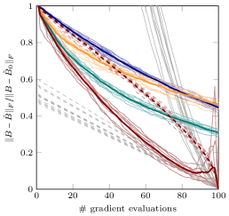
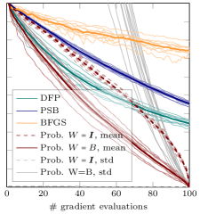
Fig. 1: Effect of parameter choice and exact vs. independent updates. Left: $10$ randomly generated linear problems with $N=100$ with eigenvalue scale $\lambda=10$. Right: Analogous problems with eigenvalue scale $\lambda=1000$. Individual experiments as thin lines, means over all $10$ experiments as thick lines. The spikes for the $W=B$ estimate at the end of the left plot are numerical artifacts caused by ill-conditioned random projections. They do not arise in the optimization setting.

How relevant is the difference between the full rank-$2M$ posterior update and a sequence of $M$ rank-$2$ updates? Figure 1 shows results from a simple conceptual experiment. For this test only, the various estimation rules are treated as ‘stand-alone’ inference algorithms, not as optimizers. Random positive definite matrices $B\in\mathbb{R}^{N\times N}$ where generated as follows: Eigenvalues $d_{i},i=1,\dots,N$ were drawn iid from an exponential distribution $p(d)=\nicefrac{{1}}{{\lambda}}\exp(-d/\lambda)$ with scale $\lambda=10$ (small eigenvalues, left plot) or $\lambda=1000$ (large eigenvalues, right plot), respectively. A random rotation matrix $Q\in SO(N)$ was drawn uniformly from the Haar measure over $SO(N)$, using the subgroup algorithm of Diaconis & Shahshahani [15], giving $B=QDQ^{\intercal}$ (where $D=\mathop{\operator@font diag}\nolimits(d)$). Projections—simulated ‘search directions’—where drawn uniformly at random as $S\in\mathbb{R}^{N\times M},s_{nm}\sim\mathcal{N}(0,1)$. For $M=1,\dots,N$, the Powell Symmetric Broyden (PSB), DFP and BFGS, as well the corresponding posterior means from Equation (15) with $W=\boldsymbol{I}$ (equal to PSB after one step) and $W=B$ (equal to DFP after one step) were used to construct point estimates $B_{M}$ for $B$. The plot shows the Frobenius norm $\|B_{M}-B\|_{F}$ between true and estimated $B$, normalised by the initial error $\|B_{0}-B\|_{F}$. All algorithms used $B_{0}=\boldsymbol{I}$.

Because directions $s$ where chosen randomly, these results say little about these algorithms as optimizers. What they do offer is an intuition for the difference between the exact rank-$2M$ posterior and repeated application of rank-$2$ Dennis-class update rules. A first observation is that, in this setup, keeping track of the dependence between consecutive search directions through $S^{\intercal}WS$ makes a big difference: For both pairs of ‘related’ algorithms PSB and $W=\boldsymbol{I}$, as well as DFP and $W=B$, the full posterior mean dominates the simpler ‘independent’ update rule. In fact, the classic secant rules do not converge to the true Hessian $B$ in this setup. The consistency argument in Section 2.2.2 only applies to estimators constructed by exact inference. The experiment shows how crucial tracking the full Gram matrix $S^{\intercal}WS$ is after $M>1$.

A second, not surprising observation is that, although both probabilistic algorithms are consistent—they converge to the correct $B$ after $N$ steps—the quality of the inferred point estimate after $M<N$ steps depends on the choice of parameters. The simpler $W=\boldsymbol{I}$ (PSB) choice performs qualitatively worse than the $W=B$ (DFP) choice.

The posterior covariances were used to compute posterior uncertainty estimates for $\|B_{M}-B\|_{F}$ (gray lines in Figure 1): The Frobenius norm can be written as $\|B_{M}-B\|^{2}_{F}=\overrightarrow{(B_{M}-B)}^{\intercal}\overrightarrow{(B_{M}-B)}$; thus the expected value of this quadratic form is

(18) $$\mathbb{E}[\overrightarrow{(B_{M}-B)}^{\intercal}\overrightarrow{(B_{M}-B)}] =\sum_{ij}V_{M,(ij)(ij)}=\sum_{ij}\frac{1}{2}(W_{M,ii}W_{M,jj}+W_{M,ij}W_{M,ij}),$$

with $W_{M}\colonequals W-WS(S^{\intercal}WS)^{-1}S^{\intercal}W$. (To be clear: for $W=B$, computing this uncertainty required the unrealistic step of giving the algorithm access to $B$, which only makes sense for this conceptual experiment). The uncertainty estimate for $W=\boldsymbol{I}$ (dashed gray lines) is all but invisible in the right hand plot because its values are very close to 0—this algorithm has a badly calibrated uncertainty measure that has no practical use as an estimate of error. The uncertainty under $W=B$ (solid gray lines), on the other hand, scales qualitatively with the size of $B$. This is because scaling $B$ by a scalar factor automatically also scales the covariance by the same factor. This has been noted before as a ‘non-dimensional’ property of BFGS/DFP [34, Eq. 6.11]. However, it is also apparent that the uncertainty estimate is too large in both plots—here by about a factor of 5. To understand why, we consider the individual terms in the sum of Equation (18) at the beginning of the inference: The ratio between the true estimation error on element $B_{ij}$ and the estimated error is

(19) $$e_{ij}^{2}=\frac{(B_{0}-B)_{ij}^{2}}{\mathbb{E}[(B_{0}-B)_{ij}^{2}]}=2\frac{B_{ij}^{2}-2B_{ij}B_{0,ij}+B_{0,ij}^{2}}{W_{ii}W_{jj}+W_{ij}^{2}}.$$

One may argue that a ‘well-calibrated’ algorithm should achieve $e_{ij}\approx 1$. A problem with the choice $W=B$ becomes apparent considering diagonal elements and $B_{0}=\boldsymbol{I}$:

(20) $$e_{ii}^{2}=\frac{(B_{ii}-1)^{2}}{B_{ii}^{2}}=\left(1-\frac{1}{B_{ii}}\right)^{2}.$$

This means the DFP prior is well-calibrated only for large diagonal elements $(B_{ii}\gg 1)$. For diagonal elements $B_{ii}\approx 1$, it is under-confident ($e_{ii}\operatorname*{\rightarrowtriangle}0$, estimating too large an error), and for very small diagonal elements $B_{ii}>0,B_{ii}\ll 1$, it can be severely over-confident ($e_{ii}\operatorname*{\rightarrowtriangle}\infty$ estimating too small an error). For off-diagonal elements and unit prior mean, the error estimate is

(21) $$e_{ij}^{2}=\frac{2B_{ij}^{2}}{B_{ij}^{2}+B_{ii}B_{jj}}=\frac{2}{1+B_{ii}B_{jj}/B_{ij}^{2}}\qquad\text{for }i\neq j.$$

For positive definite $B$, $e_{ij}^{2}<1$ off the diagonal holds because, for such matrices, $B_{ij}^{2}<B_{ii}B_{jj}$ (see e.g. [28, Corollary 7.1.5]), but of course $e_{ij}^{2}$ can still be very small or even vanish, e.g. for diagonal matrices. It is possible to at least fix the over-confidence problem, using the degree of freedom in Corollary 5 to scale the prior covariance to $W=\theta^{2}B$ with $\theta=\lambda_{\min}/(\lambda_{\min}-1)$, using $\lambda_{\min}$, the smallest eigenvalue of $B$. This at least ensures $e_{ij}\leq 1\;\forall(i,j)$.

Interestingly, setting $W=B-B_{0}$ (which gives the SR1 rule after the first observation, but not after subsequent ones) gives $e_{ii}^{2}=1$, and $e_{ij}<1$ for $i\neq j$. It also has the property that norm of the true $B$ under this prior is

(22) $$\overrightarrow{(B-B_{0})}^{\intercal}((B-B_{0})\mathchoice{{\ooalign{$\displaystyle\otimes$\cr\hfil$\displaystyle\ominus$\hfil\cr}}}{{\ooalign{$\textstyle\otimes$\cr\hfil$\textstyle\ominus$\hfil\cr}}}{{\ooalign{$\scriptstyle\otimes$\cr\hfil$\scriptstyle\ominus$\hfil\cr}}}{{\ooalign{$\scriptscriptstyle\otimes$\cr\hfil$\scriptscriptstyle\ominus$\hfil\cr}}}(B-B_{0}))^{-1}\overrightarrow{(B-B_{0})}=\overrightarrow{\boldsymbol{I}}^{\intercal}\overrightarrow{\boldsymbol{I}}=N,$$

so the true $B$ is exactly one standard deviation away from the mean under this prior. These properties suggest this covariance, which will be called standardized norm covariance, for further investigation in §4, which addresses the question: Is it possible to construct a linear solver that, without ‘cheating’ (using $B$ or $H$ explicitly in the covariance), has a well-calibrated uncertainty measure, and can thus meaningfully estimate the error of its computation; ideally, without major cost increase?

3.2 Structure of the Gram matrix

The above established that, treated as inference rules for matrices, general Dennis rules are probabilistically exact only after one rank-1 observation $y=Bs$. How strong is the error thus introduced? In fact, as the following lemma shows, there are choices of search directions $S$ for which the existing algorithms do become exact probabilistic inference.

Lemma 6 (proof in Appendix A.3).

If the Gram matrix $S^{\intercal}WS$ is a diagonal matrix (i.e., if the search directions $S\in\mathbb{R}^{N\times M}$ are conjugate under the covariance parameter $W$), then the $M$ repeated rank-2 update steps of classic secant-rule implementations result in an estimate that is equal to the posterior mean under exact probabilistic Gaussian inference from $(Y,S)$. (The equivalent statement for inverse updates requires conjugacy of the $Y$ under $W$).

So a cheap, probabilistic optimizer can be constructed by choosing search directions conjugate under $W$. The following reformulation of a previously known Lemma shows that, in fact, both the BFGS and DFP update rules have this property.

Lemma 7 (additional proof in Appendix A.4).

For linear problems $Bx=b$ with symmetric positive definite $B$ and exact line searches, under the DFP covariance $W=B$, and linesearches along the inverse of the posterior mean of the Gaussian belief, the Gram matrix is diagonal. Analogously for inverse updates: For inference on $H=B^{-1}$ under the BFGS covariance $W=H$ on the same linear optimization problem and linesearches along the posterior mean over $H$, the Gram matrix is diagonal.

The following result by Nazareth [32] establishes that, for linear problems, the inference interpretation for BFGS transfers directly to the conjugate gradient (CG) method of Hestenes & Stiefel [27].

Theorem 8 (Nazareth [32]).

For linear optimization problems as defined in Lemma 7, BFGS inference on $H$ with scalar prior mean, $H_{0}=\alpha\boldsymbol{I},\alpha\in\mathbb{R}$, is equivalent to the conjugate gradient algorithm in the sense that the sequence of search directions is equal: $s_{i}^{\text{BFGS}}=s_{i}^{\text{CG}}$.

The connection between BFGS and CG is intuitive within the probabilistic framework: BFGS uses $W=H$, so its mean estimate $H_{M}$ is the ‘best guess’ for $H$ under (the minimizer of) the norm $\overrightarrow{(H-H_{M})}^{\intercal}(H\mathchoice{{\ooalign{$\displaystyle\otimes$\cr\hfil$\displaystyle\ominus$\hfil\cr}}}{{\ooalign{$\textstyle\otimes$\cr\hfil$\textstyle\ominus$\hfil\cr}}}{{\ooalign{$\scriptstyle\otimes$\cr\hfil$\scriptstyle\ominus$\hfil\cr}}}{{\ooalign{$\scriptscriptstyle\otimes$\cr\hfil$\scriptscriptstyle\ominus$\hfil\cr}}}H)^{-1}\overrightarrow{(H-H_{M})}$, and its iterated estimate $x_{M}$ is the best rank-$M$ estimate for $x$ when the error is measured as $(x-x_{M})^{\intercal}W^{-1}(x-x_{M})=(x-x_{M})^{\intercal}B(x-x_{M})$. Minimizing this quantity after $M$ steps is a well-known characterisation of CG [34, Eq. 5.27].

Theorem 8 implies that, describing BFGS in terms of Gaussian inference also gives a Gaussian interpretation for CG ‘for free’. From the probabilistic perspective, and exclusively for linear problems, CG is ‘just’ a compact implementation of iterated Gaussian inference on $H$ from $p(H)=\mathcal{N}(H;\boldsymbol{I},H\mathchoice{{\ooalign{$\displaystyle\otimes$\cr\hfil$\displaystyle\ominus$\hfil\cr}}}{{\ooalign{$\textstyle\otimes$\cr\hfil$\textstyle\ominus$\hfil\cr}}}{{\ooalign{$\scriptstyle\otimes$\cr\hfil$\scriptstyle\ominus$\hfil\cr}}}{{\ooalign{$\scriptscriptstyle\otimes$\cr\hfil$\scriptscriptstyle\ominus$\hfil\cr}}}H)$, with search directions along $H_{M}F(x_{M})=H_{M}(Bx_{M}-b)$. This observation has conceptual value in itself (the natural question, left open here, is what it implies for the nonparametric extensions of CG). But Theorem 8, among other things, also implies the following helpful properties for the search directions $s_{i}$ chosen by, and gradients $F_{i}$ ‘observed’ by the (scalar prior mean) BFGS algorithm. They are all well-known properties of the conjugate gradient method (e.g. [34, Thm. 5.3]). In the following, generally assume that the algorithm has not converged at step $M<N$, and remember that the $F_{M}=Bx_{M}-b$ are the residuals (gradients of $f(x)=\nicefrac{{1}}{{2}}x^{\intercal}Bx-x^{\intercal}x$) after $M$ steps, which form $y_{M}=F_{M}-F_{M-1}$.

• the set of evaluated gradients / residuals is orthogonal:

  (23) $$F_{i}^{\intercal}F_{j}=0\text{ for $i\neq j$ and $i,j<N$}$$

• the gradients (and thus $Y$) span the Krylov subspaces generated by $(B,b)$:

  (24) $$\operatorname{span}\{F_{0},F_{1},\dots,F_{M}\}=\operatorname{span}\{F_{0},BF_{0},\dots,B^{M}F_{0}\}$$

• line searches and gradients span the same vector space:

  (25) $$\operatorname{span}\{s_{0},s_{1},\dots,s_{M}\}=\operatorname{span}\{F_{0},BF_{0},\dots,B^{M}F_{0}\}$$

3.3 Discussion

We have established a probabilistic interpretation of the Dennis class of quasi-Newton methods, and the CG algorithm, as Gaussian inference: The Dennis class can be seen as Gaussian posterior means after the first line search (Corollary 4), but this connection extends to multiple search directions only if the search directions are conjugate under prior covariance (Lemma 6). For linear problems, this is the case for the DFP, BFGS update rules (Lemma 7). Since BFGS is equivalent to CG on linear problems (Lemma 8), this also establishes a probabilistic interpretation for linear CG. These results offer new ways of thinking about linear solvers, in terms of solving an inference problem by collecting information and building a model, rather than by designing a dynamic process converging to the minimum of a function. It is intriguing that, from this vantage point, the extremely popular CG / BFGS methods look less well-calibrated than one may have expected (§3.1).

The obvious next question is, can one design explicitly uncertain linear solvers with a reasonably well-calibrated posterior? In addition to the scaling issues, a challenge is that, for BFGS / CG, the prior covariance $W=H$ is only an implicit object. After $M<N$ steps, there exists a $\nicefrac{{1}}{{2}}(N-M)(N-M+1)$-dimensional cone of positive definite covariance matrices fulfilling $WY=S$ (and, additionally, a scalar degree of freedom inherent to the Dennis class). How do we pick a point in this space?

4 Constructing explicit posteriors

The remainder will focus exclusively on inference on $H=B^{-1}$, on inverse update rules, priors $p(H)=\mathcal{N}(\overrightarrow{H};\overrightarrow{H}_{0},W\mathchoice{{\ooalign{$\displaystyle\otimes$\cr\hfil$\displaystyle\ominus$\hfil\cr}}}{{\ooalign{$\textstyle\otimes$\cr\hfil$\textstyle\ominus$\hfil\cr}}}{{\ooalign{$\scriptstyle\otimes$\cr\hfil$\scriptstyle\ominus$\hfil\cr}}}{{\ooalign{$\scriptscriptstyle\otimes$\cr\hfil$\scriptscriptstyle\ominus$\hfil\cr}}}W)$. As pointed out in §1.2, these arise from the direct rules under exchange of $S$ and $Y$: Given $(S,Y)\in\mathbb{R}^{N\times M}$, the posterior belief is $p(H\,|\,S,Y)=\mathcal{N}(\overrightarrow{H};\overrightarrow{H}_{M},W_{M}\mathchoice{{\ooalign{$\displaystyle\otimes$\cr\hfil$\displaystyle\ominus$\hfil\cr}}}{{\ooalign{$\textstyle\otimes$\cr\hfil$\textstyle\ominus$\hfil\cr}}}{{\ooalign{$\scriptstyle\otimes$\cr\hfil$\scriptstyle\ominus$\hfil\cr}}}{{\ooalign{$\scriptscriptstyle\otimes$\cr\hfil$\scriptscriptstyle\ominus$\hfil\cr}}}W_{M})$ with

(26) $$H_{M} =H_{0}+(S-H_{0}Y)(Y^{\intercal}WY)^{-1}Y^{\intercal}W+WY(Y^{\intercal}WY)^{-1}(S-H_{0}Y)^{\intercal}$$

$$\qquad-WY(Y^{\intercal}WY)^{-1}[Y^{\intercal}(S-H_{0}Y)](Y^{\intercal}WY)^{-1}Y^{\intercal}W$$

$$W_{M} =W-WY(Y^{\intercal}WY)^{-1}Y^{\intercal}W.$$

Recall from Sections 1.2 and Corollary 5 that, cast as an inverse update, BFGS (CG) arises from the prior $p(H)=\mathcal{N}(H;\boldsymbol{I},\theta^{2}(H\mathchoice{{\ooalign{$\displaystyle\otimes$\cr\hfil$\displaystyle\ominus$\hfil\cr}}}{{\ooalign{$\textstyle\otimes$\cr\hfil$\textstyle\ominus$\hfil\cr}}}{{\ooalign{$\scriptstyle\otimes$\cr\hfil$\scriptstyle\ominus$\hfil\cr}}}{{\ooalign{$\scriptscriptstyle\otimes$\cr\hfil$\scriptscriptstyle\ominus$\hfil\cr}}}H))$ for arbitrary $\theta\in\mathbb{R}_{+}$.

4.1 Fitting covariance matrices

Equations (6), (7) show that both the BFGS and DFP priors in principle require access to $H$. As noted above, for this mean estimate it is implicitly feasible to use $W=H$, because this computation only requires observed projections $WY=HY=S$. Computing the covariance under $W=H$, however, can only be an idealistic goal: After $M$ steps, only a sub-space of rank $\frac{1}{2}(N(N+1)-(N-M)(N-M+1))$ of the elements of $H$ is identified. To see this explicitly, consider the singular value decomposition $Y=Q\Sigma U^{\intercal}$, which defines a symmetric positive definite $T\in\mathbb{R}^{N\times N}$ through $W=QTQ^{\intercal}$. This notation gives

(27) $$W_{M}=W-WY(Y^{\intercal}WY)^{-1}Y^{\intercal}W=Q(T-T\Sigma(\Sigma^{\intercal}T\Sigma)^{-1}\Sigma^{\intercal}T)Q^{\intercal}.$$

Considering the structure of $\Sigma$, one can write $T$ in terms of block matrices

(28) $$T=\begin{pmatrix}T_{++}&T_{+-}\\ T_{-+}&T_{--}\end{pmatrix}\qquad\text{then}\qquad W_{M}=Q\begin{pmatrix}0&0\\ 0&T_{--}-T_{-+}T_{++}^{-1}T_{+-}\end{pmatrix}Q^{\intercal},$$

with $T_{++}\in\mathbb{R}^{M\times M},T_{-+}=T_{+-}^{\intercal}\in\mathbb{R}^{M\times(N-M)},T_{--}\in\mathbb{R}^{(N-M)\times(N-M)}$ (and positive definite $T_{++}$, a principal block of the positive definite $T$). Observing $(S,Y)$, exactly identifies $[T_{++},T_{+-}]^{\intercal}=QSU^{\intercal}D^{-1}$, and provides no information at all about $T_{--}$.

A primary goal in designing a probabilistic linear solver is thus, at step $M<N$, to (1) identify the span of $W_{M}$, ideally without incurring additional cost, and to (2) fix the entries in the remaining free dimensions in $W_{M}$, by using some regularity assumptions about $H$. The equivalence between BFGS and CG offers an elegant way of solving problem (1), with no additional computational cost: Recall from Theorem 3 and Lemma 6 that the covariance after $M$ steps under $W=H$ is $W_{M}\mathchoice{{\ooalign{$\displaystyle\otimes$\cr\hfil$\displaystyle\ominus$\hfil\cr}}}{{\ooalign{$\textstyle\otimes$\cr\hfil$\textstyle\ominus$\hfil\cr}}}{{\ooalign{$\scriptstyle\otimes$\cr\hfil$\scriptstyle\ominus$\hfil\cr}}}{{\ooalign{$\scriptscriptstyle\otimes$\cr\hfil$\scriptscriptstyle\ominus$\hfil\cr}}}W_{M}$ with

(29) $$W_{M}=W-\sum_{i}^{M}\frac{Wy_{i}(Wy_{i})^{\intercal}}{s_{i}^{\intercal}y_{i}}=W-\sum_{i}^{M}\frac{s_{i}s_{i}^{\intercal}}{s_{i}^{\intercal}y_{i}}=W-S(S^{\intercal}Y)^{-1}S^{\intercal},$$

Because, by Equation (25) the vector-space spanned by $S$ is identical to that spanned by the orthogonal gradients, we can write the space of all symmetric positive semidefinite matrices $W$ with the property $WY=S$ as

(30) $$W(\Omega)=S(S^{\intercal}Y)^{-1}S^{\intercal}+(\boldsymbol{I}-\bar{F}\bar{F}^{\intercal})\Omega(\boldsymbol{I}-\bar{F}\bar{F}^{\intercal}),$$

with the right-orthonormal matrix $\bar{F}$ containing the $M$ normalised gradients $F_{i}/\|F_{i}\|$ in its columns, and a positive definite matrix $\Omega\in\mathbb{R}^{N\times N}$ (the effective size of the space spanned in this way is only $\mathbb{R}^{(N-M)\times(N-M)}$, so $\Omega$ is over-parameterising this space).

4.1.1 Standardized norm posteriors using conjugate gradient observations

Eq. (30) parametrises posterior covariances of the BFGS family. In light of the scaling issues of these priors discussed in §3.1, one would prefer, from the probabilistic standpoint, to use the standardized norm priors $p(H)=\mathcal{N}(H;\alpha\boldsymbol{I},(H-H_{0})\mathchoice{{\ooalign{$\displaystyle\otimes$\cr\hfil$\displaystyle\ominus$\hfil\cr}}}{{\ooalign{$\textstyle\otimes$\cr\hfil$\textstyle\ominus$\hfil\cr}}}{{\ooalign{$\scriptstyle\otimes$\cr\hfil$\scriptstyle\ominus$\hfil\cr}}}{{\ooalign{$\scriptscriptstyle\otimes$\cr\hfil$\scriptscriptstyle\ominus$\hfil\cr}}}(H-H_{0}))$, but these priors do not share BFGS/CG’s other good numerical properties. Instead, a hybrid algorithm can be constructed as follows:

1. Solve the linear problem using the conjugate gradient method. While the algorithm runs, collect $S,Y,\bar{F}$. This has storage cost of $2NM+M$ floats: Because $Y$ consists of differences between subsequent columns of $F$, it does not need to be stored explicitly, the column norms $\|F\|_{i}$ required to compute $\bar{F}$ require $M$ extra floats. The computation cost of the standard conjugate gradient algorithm is $\mathcal{O}(M)$ matrix-vector multiplications (that is, $\mathcal{O}(MN^{2})$ assuming a dense matrix), plus $\mathcal{O}(MN)$ operations for the algorithm itself (including computation of $\|F\|_{i}$).

2. Using the $(S,Y,\bar{F})$ constructed by CG, compute the standardized-norm posterior on $H$, i.e. use the prior $p(H)$ defined above, which yields a Gaussian posterior with mean and covariance

   (31) $$H_{M} =H_{0}+(S-H_{0}Y)(Y^{\intercal}(S-H_{0}Y))^{-1}(S-H_{0}Y)^{\intercal}$$

   (32) $$=\alpha\boldsymbol{I}-(S-\alpha Y)(Y^{\intercal}S-\alpha Y^{\intercal}Y)^{-1}(S-\alpha Y)^{\intercal}\qquad\text{and}$$

   (33) $$W_{M} =(H-H_{0})-(S-H_{0}Y)(Y^{\intercal}(S-H_{0}Y))^{-1}(S-H_{0}Y)^{\intercal}$$

   (34) $$=S(S^{\intercal}Y)^{-1}S^{\intercal}+(\boldsymbol{I}-\bar{F}\bar{F}^{\intercal})\Omega(\boldsymbol{I}-\bar{F}\bar{F}^{\intercal})-\alpha\boldsymbol{I}$$

   $$\qquad-(S-\alpha Y)(Y^{\intercal}S-\alpha Y^{\intercal}Y))^{-1}(S-\alpha Y)^{\intercal}.$$

   A prerequisite for this is to choose $\alpha<\lambda_{\min}(H)$, less than the smallest eigenvalue of $H$, to ensure that $W=H-H_{0}$ is positive definite. But $\lambda_{\min}(H)=1./\lambda_{\max}(B)$, which can be estimated efficiently (and without additional cost) from the $\|F\|_{i}$. Another minor hurdle is that Equations (32) & (34) require the inverse of $S^{\intercal}Y-\alpha Y^{\intercal}Y$. The columns of $Y$ are $Y_{i}=F_{i}-F_{i-1}$, so, because conjugate gradient constructs orthogonal gradients, $Y^{\intercal}Y$ is a symmetric tridiagonal matrix, $Y_{i}^{\intercal}Y_{j}=\delta_{ij}(\|F_{i}\|^{2}+\|F_{i-1}\|^{2})+(\delta_{i(j-1)}+\delta_{(i+1)j})\|F_{i}\|^{2}$, and $S^{\intercal}Y$ is diagonal because the $S$ are conjugate under $B$. So the entire Gram matrix is tridiagonal, and the $M$ linear problems in $(Y^{\intercal}S-\alpha YY^{\intercal})^{-1}(S-\alpha Y)^{\intercal}$ can be solved in $\mathcal{O}(M^{2})$, e.g. using the Thomas algorithm [7, Alg. 4.3]

3. estimate $\Omega$ according to some rule. §4.2 proposes several rules of $\mathcal{O}(M)$ cost.

While there is a vague connection between the standardized norm prior and the SR1 algorithm by Corollary 5, the algorithm described above is quite different from the SR1 method. It uses search directions constructed by BFGS/CG, and its update rule uses the exact Gram matrix, not the repeated rank-1 updates that give SR1 its name.

Computational cost

The computation overhead of constructing this posterior mean and covariance, after running the conjugate gradient algorithm, is $\mathcal{O}(M^{2})$, which is small compared even to the internal $\mathcal{O}(MN)$ cost of CG, let alone the $\mathcal{O}(MN^{2})$ for the matrix-vector multiplications in CG. Storing the posterior mean and covariance requires $\mathcal{O}(NM)$ space, which is feasible even for relatively large problems. Crucially, retaining the covariance adds almost no overhead to storing the mean alone.

4.2 Estimation rules

uniformly distributed eigenvalues
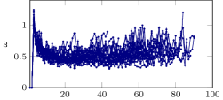
exponentially distributed eigenvalues
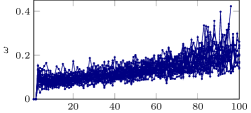
structured eigenvalue spectrum

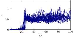
Fig. 2: Fitting posterior uncertainty during iterative solution of linear problems, for three different generative processes of $B$. Each plot shows results from 20 randomly generated experiments with, top row: uniformly, middle row: exponentially distributed eigenvalues; bottom row: structured eigenvalue spectrum (details in text). Left: Residual (gradient) $Bx-b$ as a function of number of line searches. Right: projections $\omega=s_{M}^{\intercal}F_{M-1}$, whose regular structure is used for estimating $W(\Omega)$.

The remaining step is to find estimates for $\Omega$. It is clear that there are myriad options for fixing such rules. For an initial evaluation, we adopt the perhaps simplistic, but straightforward approach of estimating $\Omega$ to a scalar matrix $\Omega=\omega^{2}\boldsymbol{I}$ (one way to motivate this is to argue that, at step $M$, future line searches $s_{M+i}$ will point in an unknown direction in the span of $\boldsymbol{I}-\bar{F}\bar{F}^{\intercal}$, so it makes sense to not prefer any direction in the choice of $\Omega$).

A natural idea is to use regularity structure on quantities already computed during the run of the conjugate gradient algorithm: Assume the algorithm is currently at step $T$. If, at step $M<T$ we had tried to predict the Gram matrix diagonal element $y_{M+1}^{\intercal}Wy_{M+1}=-s_{M+1}^{\intercal}F_{M}$ using the structure for $W$ described above, we would have predicted, because $F_{M}$ is known to be in the span of $S$, and orthogonal to $(\boldsymbol{I}-\bar{F}\bar{F}^{\intercal})$,

(35) $$y_{M+1}^{\intercal}Wy_{M+1} =F_{M}^{\intercal}S(S^{\intercal}Y)^{-1}S^{\intercal}F_{M}+F_{M+1}^{\intercal}\Omega F_{M+1}$$

(36) $$-s_{M+1}^{\intercal}F_{M} =-\sum_{i=1}^{M}\frac{(F_{M}^{\intercal}s_{i})^{2}}{s_{i}^{\intercal}F_{i-1}}+\omega^{2}\|F_{M+1}\|^{2},$$

(37) $$\text{and thus }\qquad\omega^{2} =\|F_{M+1}\|^{-2}\left[\sum_{i=1}^{M}\frac{(F_{M}^{\intercal}s_{i})^{2}}{s_{i}^{\intercal}F_{i-1}}-s_{M+1}^{\intercal}F_{M}\right].$$

$\|F_{M+1}\|$ can be estimated from the norm of preceding gradients. The second term on the right hand side of Equation (37) is known at step $M$. The first term of the right hand side can be estimated by regression, in ways further explored below.

First, to confirm that $\omega$ indeed tends to have regular structure related to the eigenvalue spectrum of $H$, Figure 2, right column, shows $\omega_{i}$ for $i=1,\dots,M$ during runs of CG on 20 linear problems, sampled from three different generative processes for $B=QDQ^{\intercal}\in\mathbb{R}^{200\times 200}$. In each case, orthonormal matrices where drawn uniformly from the Haar measure over $SO(N)$ as in §3.1. For the top row of Figure 2, the eigenvalues (elements of $D=\mathop{\operator@font diag}\nolimits(d)$) where drawn uniformly from $p(d_{i})=U(0,10)$ (the uniform distribution over $[0,10]$). For the middle row, eigenvalues where drawn from the exponential distribution $p(d_{i})=\nicefrac{{1}}{{\lambda}}\exp(-\nicefrac{{d_{i}}}{{\lambda}})$ with scale $\lambda=10/\log 2$ (giving a median eigenvalue of $10$). Finally, for the bottom row, eigenvalues where drawn from a structured process, with $d_{i}$ for $i=1,\dots,20$ drawn from $p(d)=U(0,10^{3})$, and $d_{i}$ for $i=21,\dots,200$ drawn from $p(d)=U(0,10)$ (i.e. the corresponding eigenvalues of $H$ lie non-uniformly in $[0,10^{-3}]$ and $[0,0.1]$). Clear structure is visible in all cases. Using these observations, several different regression schemes for $\omega$ can be adopted.

• A simple baseline is a stationary model for the $\omega_{i}$. This was used to construct error estimates in Figures 3 to 5 (in gray for the middle and bottom row, black for the top row). Of course, if the eigenvalues of $B$ are uniformly distributed in the top row, the eigenvalues of $H$ (their inverses) are not.

• A slightly more elaborate model is a linear trend with noise: $\omega_{i}=ai+b+n$ (with $n\sim\mathcal{N}(0,\sigma^{2})$). Linear regression on the values of $\omega_{i}$ can be performed in $\mathcal{O}(M)$. We can then set $\Omega=\bar{\omega}\boldsymbol{I}$ with $\bar{\omega}=aN+b$ the expected largest value of $\omega_{i}$ (i.e. a noisy upper bound). This approach was used to construct the (black) error estimates in the middle rows of Figures 3 to 5.

• Finally, if structural knowledge is available, e.g. that the first $L$ eigenvalues of $B$ are $\alpha$ times larger than the later ones, on may use the stationary rule from above, but explicitly multiply the estimate $\omega$ by $\alpha$ for the first $L$ steps. This may seem contrived, but in fact it is not uncommon in applications to know an effective number of degrees of freedom in $B$. For example, in nonparametric least-squares regression with a very large number of $N$ data points distributed approximately uniformly over a range of width $\rho$, using an RBF kernel of length scale $\lambda$, the model’s number of degrees of freedom is $L=\rho/(2\pi\lambda)$ [38, Eq. 4.3]. This rule was used to construct (black) error estimates in the bottom rows of Figures 3 to 5.

4.3 Estimating quantities of interest

uniformly distributed eigenvalues
exponentially distributed eigenvalues
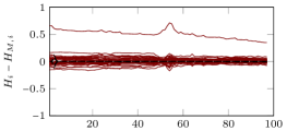
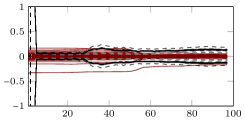
structured eigenvalue spectrum

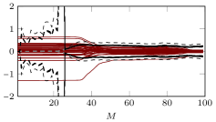
Fig. 3: Error estimation on $H$. Posterior mean (solid red) and one standard deviation (dashed black, gray). Left: BFGS/CG prior. Right: Standardized norm prior, from CG observations. Rows as in Figure 2. The cut-off error bars in the bottom right plot rise up to values $<6$.

uniformly distributed eigenvalues
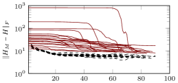
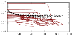
exponentially distributed eigenvalues
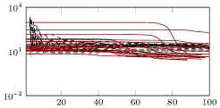
structured eigenvalue spectrum

Fig. 4: True and estimated norm error $\|H-H_{M}\|_{F}$. Posterior mean (red) and one standard deviation (black, gray). Left: BFGS/CG prior. Right: Standardized norm prior, from CG observations. Rows as in Figure 2.

uniformly distributed eigenvalues
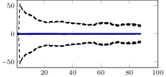
exponentially distributed eigenvalues
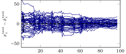
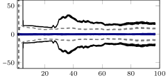
structured eigenvalue spectrum

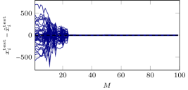
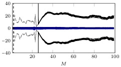
Fig. 5: Estimating solutions to $Bx^{\prime}=b^{\prime}$. Element-wise error on a single test vector $x_{\text{test}}$. True error in blue. Error estimate with stationary model for $\omega$ in gray. Error estimate for model-specific estimate for $\omega$ (as in Figure 2) in black. Left: BFGS/CG prior. Right: Standardized norm prior, from CG observations. Rows as in Figure 2.

This final part demonstrates a few example uses of the Gaussian posterior $p(H)=\mathcal{N}(\overrightarrow{H};\overrightarrow{H}_{M},W_{M}\mathchoice{{\ooalign{$\displaystyle\otimes$\cr\hfil$\displaystyle\ominus$\hfil\cr}}}{{\ooalign{$\textstyle\otimes$\cr\hfil$\textstyle\ominus$\hfil\cr}}}{{\ooalign{$\scriptstyle\otimes$\cr\hfil$\scriptstyle\ominus$\hfil\cr}}}{{\ooalign{$\scriptscriptstyle\otimes$\cr\hfil$\scriptscriptstyle\ominus$\hfil\cr}}}W_{M})$ on $H$ constructed by the BFGS / CG method. Figures 3 to 5 show three such uses, explained below. Each row of this figure uses data from one of the experiments shown in the corresponding row of Figure 2.

4.3.1 Estimating $H$ itself

The most obvious question is how far the estimate $H_{M}$ for $H$ after $M$ steps is from the true $H$. This distance is estimated directly by the Gaussian posterior of Equation (26). The marginal distribution on any linear projection $A\overrightarrow{H}$ is $\mathcal{N}(A\overrightarrow{H};A\overrightarrow{H}_{M},A(W_{M}\mathchoice{{\ooalign{$\displaystyle\otimes$\cr\hfil$\displaystyle\ominus$\hfil\cr}}}{{\ooalign{$\textstyle\otimes$\cr\hfil$\textstyle\ominus$\hfil\cr}}}{{\ooalign{$\scriptstyle\otimes$\cr\hfil$\scriptstyle\ominus$\hfil\cr}}}{{\ooalign{$\scriptscriptstyle\otimes$\cr\hfil$\scriptscriptstyle\ominus$\hfil\cr}}}W_{M})A^{\intercal})$. In particular, the marginal distribution on each element $H_{ij}$ is a scalar Gaussian

(38) $$p(H_{ij}\,|\,S_{M},Y_{M})=\mathcal{N}[H_{ij};H_{M,ij},\nicefrac{{1}}{{2}}(W_{M,ii}W_{M,jj}+W_{M,ij}^{2})].$$

Figure 3 shows this error estimate for 40 elements of one particular $H$ (drawn uniformly at random from the $4\cdot 10^{4}$ elements of the $200\times 200$ matrix). The estimate arising from the uniform estimation rule for $\omega$ from Section 4.2 is shown in gray in each panel (black for the top panel). The same quantity, estimated with the linear regression and structured estimation rules from Section 4.2 are shown in black in the middle and bottom row, respectively. The left column of the figure shows results from the BFGS/CG prior, the right column shows results using the standardized norm prior on data constructed with the CG algorithm as described in §4.1.1. As expected from the argument in §3.1, the BFGS estimates are regularly considerably too small, while the standardized-norm estimates have a meaningful width. The error estimators have varying behaviour. For the exponential eigenvalue spectrum, the estimator fluctuates strongly in the first few steps before settling to a good value (this could be corrected using a regularizer, left out here to not bias the results). For the structured-eigenvalues problems, the region around the step from small to large eigenvalues is problematic. But overall, they do provide a meaningful notion of error. In particular, they are rarely too small. For most uses of statistical error estimators, it is better to be too conservative (too large) than to be too confident. Of course, it would be great if future research would find better calibrated error estimates.

As explained in Equation (18), the same error estimates can also be collapsed into an error estimate on the norm $\|H-H_{M}\|_{F}$. Figure 4 shows results from such an experiment, for the 20 different $H$’s from Figure 2. The quantitative results are similar to the previous figure, but this figure more clearly shows the difference between the baseline (gray) and exponential, structured error estimates (black), and the behaviour of the estimated errors relative to the varying norms of the drawn $H$’s.

4.3.2 Estimating solutions for new linear problems

An obvious use for the estimate for $H$ found by CG / BFGS when solving one linear problem $Bx=b$ is as an instantaneous solution estimate for other linear problems $Bx_{\text{test}}=b_{\text{test}}$. The left and middle columns of Figure 5 shows this use. In each case, an $x_{\text{test}}$ was drawn from $\mathcal{N}(x;0,10\boldsymbol{I})$, and the corresponding $b_{\text{test}}=Bx_{\text{test}}$ presented to the algorithm. Since $x_{\text{test}}=Hb_{\text{test}}$ is a linear projection of $H$, the posterior marginal on $x_{\text{test}}$ is also Gaussian $p(x_{\text{test}}\,|\,S_{M},Y_{M})=\mathcal{N}(x_{\text{test}},H_{M}b_{\text{test}},\Sigma)$, and has covariance matrix elements

(39) $$\operatorname{cov}(x_{\text{test},i},x_{\text{test},j})=\Sigma_{ij}=\nicefrac{{1}}{{2}}(W_{ij}x_{\text{test}}^{\intercal}Wx_{\text{test}}+(Wx_{\text{test}})_{i}(W_{\text{test}})_{j}.$$

Figure 4 shows the true errors on the elements of $x_{\text{test}}$ in blue, and the estimated marginal errors (the diagonal elements of $\Sigma$) in black for the stationary, linear, structured models, respectively (and, as in previous figures, the stationary model in gray in the two non-stationary cases). More drastically than the previous ones, these figures show that the BFGS posterior can severely underestimate the error on elements of $x_{\text{test}}$, while the standardized norm prior at least provides outer bounds (albeit sometimes quite loose ones).

Remark on convergence

The error on $x_{\text{test}}$ does not always collapse over the course of finding $x$. This says more about CG as such than about its probabilistic interpretation: CG does not aim to construct $H$, but only to find $x_{*}$. For simplicity of exposition, we have assumed that $H=B^{-1}$ exists, and CG requires the full $N$ steps to converge, thus identifying $B$ and $H$. In general, CG regularly converges much earlier. For an intuition, consider the special case where $x_{0}=0$ and $b=[1,\dots,1,0,0,\dots,0]$ consists of $K$ consecutive ones and $N-K$ zeros. The CG/BFGS algorithm will never explore the lower $(N-K)\times(N-K)$ block of $H$, which may contain arbitrary numbers. If the primary aim is not $x_{*}=Hb$ but $H$ itself, a more elaborate course is needed; e.g. choosing several $b$ to span a space of interest over $H$. It is an interesting open question whether the probabilistic interpretation can be used to actively collapse the uncertainty on $H$ in a typically more efficient way than established matrix inversion methods like Gauss-Jordan (which is also a conjugate direction method [27]).

5 Conclusion & outlook

This text developed a probabilistic interpretation of iterative solvers for linear problems $Bx=b$ with symmetric $B$. The Dennis family of secant updates can be derived as the posterior mean of a parametric Gaussian model after one rank-1 observation. For rank $M$ observations, the match between these updates and Gaussian inference only holds if the search directions are conjugate under the prior covariance. This is the case for the DFP direct and BFGS inverse updates rules. Their equivalence to CG in the linear case makes them particularly interesting. However, it also became apparent that, from a inference perspective, the BFGS rule does not yield a well-scaled error measure.

As a first step toward a better scaled Gaussian belief, the standardized norm covariance, was proposed. It is inspired by the SR1 rule, but leads to probabilistic corrections in the form of off-diagonal terms, and can be used with data produced by the CG algorithm, thus retaining the good numerical properties of that method. The space of possible covariance matrices consistent with the resulting mean is a sub-space of the positive definite cone, which collapses during the run of the algorithm (the same holds for the BFGS / CG method). Several possible estimation rules for choosing elements in this space of covariances where proposed, arising from different structural assumptions over $H$. The resulting Gaussian posterior provides joint uncertainty estimates on the elements of $H$, and all linear projections of $H$, in particular of other linear problems $x_{\text{test}}=Hb_{\text{test}}$. This adds functionality to the conjugate gradient method, at a computational overhead much smaller than the cost of CG itself.

The implications for nonlinear optimization methods of both the quasi-Newton and CG families remain interesting open questions. For example, clearly the conjugacy assumption implicit in the Dennis class members is inconsistent with the probabilistic interpretation. This was already noted by Hennig & Kiefel [25, 26], who also proposed using a nonparametric Gaussian formulation to give a more explicit inference interpretation to nonlinear optimization. This left questions regarding the choice of prior covariance, which are only made more pressing by the results presented here. Another direction is inference from noisy evaluations, in which case the posterior covariance does not collapse to zero after finitely many steps of optimization, not even in the linear case. Some related results where previously discussed in [24], but the study of probabilistic numerical optimization remains at an early stage.

Appendix A Proofs for results from main text

Throughout the appendix, the notation $\Delta=Y-B_{0}S$ will be used to represent the residual.

A.1 Proof for Lemma 2

Because the operator $\Gamma$ maps $\sum_{k\ell}\Gamma_{ij,k\ell}A_{k\ell}=\nicefrac{{1}}{{2}}(A_{ij}+A_{ji})$ for all $A$, its elements can be written as $\Gamma_{ij,k\ell}=\nicefrac{{1}}{{2}}(\delta_{ik}\delta_{j\ell}+\delta_{i\ell}\delta_{jk})$, using Kronecker’s $\delta$ function. We also note that Gaussians are closed under linear operations (see e.g. [2, Eq. 2.115]: $p(B)=\mathcal{N}(\overrightarrow{B};\overrightarrow{B}_{0},V)$ implies $p(\Gamma\overrightarrow{B})=\mathcal{N}(\Gamma\overrightarrow{B};\overrightarrow{B}_{0},\Gamma V\Gamma^{\intercal})$. We complete the proof by observing that

(40) $$(\Gamma(W\otimes W)\Gamma^{\intercal})_{ij,k\ell} =\sum_{ab,cd}\nicefrac{{1}}{{4}}(\delta_{ia}\delta_{jb}+\delta_{ib}\delta_{ja})(\delta_{kc}\delta_{\ell d}+\delta_{kd}\delta_{\ell c})W_{ac}W_{bd}$$

(41) $$=\nicefrac{{1}}{{4}}(W_{ik}W_{j\ell}+W_{i\ell}W_{jk}+W_{jk}W_{i\ell}+W_{j\ell}W_{ik})$$

(42) $$=\nicefrac{{1}}{{2}}(W_{ik}W_{j\ell}+W_{i\ell}W_{jk})\qquad\qquad\end@proof$$

A.2 Proof for Theorem 3

To be shown: Given $p(B)=\mathcal{N}(\overrightarrow{B};\overrightarrow{B}_{0},W\mathchoice{{\ooalign{$\displaystyle\otimes$\cr\hfil$\displaystyle\ominus$\hfil\cr}}}{{\ooalign{$\textstyle\otimes$\cr\hfil$\textstyle\ominus$\hfil\cr}}}{{\ooalign{$\scriptstyle\otimes$\cr\hfil$\scriptstyle\ominus$\hfil\cr}}}{{\ooalign{$\scriptscriptstyle\otimes$\cr\hfil$\scriptscriptstyle\ominus$\hfil\cr}}}W)$, the posterior from the likelihood $\delta(Y-BS)=\lim_{\Lambda\operatorname*{\rightarrowtriangle}0}\mathcal{N}(Y;(\boldsymbol{I}\otimes S)B,\Lambda)$, with $Y,S\in\mathbb{R}^{N\times M}$ and $\operatorname{rk}(S)=M$ has mean (with $\Delta=Y-B_{0}S$)

(43) $$B_{M} =B_{0}+\Delta(S^{\intercal}WS)^{-1}WS^{\intercal}+WS(S^{\intercal}WS)^{-1}\Delta^{\intercal}$$

$$\quad-WS(S^{\intercal}WS)^{-1}(S^{\intercal}\Delta)(S^{\intercal}WS)^{-1}S^{\intercal}W,$$

and covariance

(52) $$V_{M} =(W-WS(S^{\intercal}WS)^{-1}S^{\intercal}W)\mathchoice{{\ooalign{$\displaystyle\otimes$\cr\hfil$\displaystyle\ominus$\hfil\cr}}}{{\ooalign{$\textstyle\otimes$\cr\hfil$\textstyle\ominus$\hfil\cr}}}{{\ooalign{$\scriptstyle\otimes$\cr\hfil$\scriptstyle\ominus$\hfil\cr}}}{{\ooalign{$\scriptscriptstyle\otimes$\cr\hfil$\scriptscriptstyle\ominus$\hfil\cr}}}(W-WS(S^{\intercal}WS)^{-1}S^{\intercal}W).$$

We begin with the posterior mean (43). From Equation (10), it has the form (with the prior covariance $V=W\mathchoice{{\ooalign{$\displaystyle\otimes$\cr\hfil$\displaystyle\ominus$\hfil\cr}}}{{\ooalign{$\textstyle\otimes$\cr\hfil$\textstyle\ominus$\hfil\cr}}}{{\ooalign{$\scriptstyle\otimes$\cr\hfil$\scriptstyle\ominus$\hfil\cr}}}{{\ooalign{$\scriptscriptstyle\otimes$\cr\hfil$\scriptscriptstyle\ominus$\hfil\cr}}}W$)

(53) $$\boldsymbol{B}_{0}+V(\boldsymbol{I}\otimes S)[(\boldsymbol{I}\otimes S^{\intercal})V(\boldsymbol{I}\otimes S)]^{-1}\overrightarrow{\Delta}.$$

A few straightforward steps establish that the $NM\times NM$ matrix to be inverted is indeed invertible for linearly independent columns of $S$, and has elements

(54) $$[(\boldsymbol{I}\otimes S^{\intercal})V(\boldsymbol{I}\otimes S)]_{ia,jb} =\nicefrac{{1}}{{2}}[W_{ij}(S^{\intercal}WS)_{ab}+(WS)_{ib}(WS)_{ja}].$$

Also, the elements of $V(\boldsymbol{I}\otimes S)$ are

(55) $$[V(\boldsymbol{I}\otimes S)]_{ij,ka}=\nicefrac{{1}}{{2}}(W_{ik}S_{ja}+W_{jk}S_{ia}).$$

So we are searching the unique matrix $X\in\mathbb{R}^{N\times M}$ satisfying

(56) $$\overrightarrow{\Delta}=[(\boldsymbol{I}\otimes S^{\intercal})V(\boldsymbol{I}\otimes S)]\overrightarrow{X}=\nicefrac{{1}}{{2}}(\overrightarrow{WXS^{\intercal}WS+WSX^{\intercal}WS}),$$

which then gives the posterior as $\nicefrac{{1}}{{2}}(WXS^{\intercal}WSWSX^{\intercal}W)$. (Because $X$ is rectangular, Equation (56) is a generalization of a Lyapunov equation. Standard solutions for such Equations do not apply directly). Instead of just presenting a solution, the following lines show a constructive proof. We first re-write Eq. (56) ($S^{\intercal}WS$ is invertible because $W$ is positive definite, and $S$ is assumed to be of rank $M$) as

(57) $$2\Delta =WXS^{\intercal}WS+WSX^{\intercal}WS,$$

(58) $$2W^{-1}\Delta(S^{\intercal}WS)^{-1} =X+SX^{\intercal}WS(S^{\intercal}WS)^{-1}.$$

Let $Q\Sigma U^{\intercal}=S$ be the singular value decomposition of $S$. That is, $Q\in\mathbb{R}^{N\times N}$ and $U\in\mathbb{R}^{M\times M}$ are orthonormal, $\Sigma\in\mathbb{R}^{N\times M}$, consisting of an upper part containing the diagonal matrix $D\in\mathbb{R}^{M\times M}$ and a lower part in $\mathbb{R}^{(N-M)\times M}$ containing on zeros. We will write $Q=[Q_{+},Q_{-}]$, where $Q_{+}\in\mathbb{R}^{N\times M}$ is a basis of the preimage of $S$, and $Q_{-}\in\mathbb{R}^{(N-M)\times M}$ is a basis of the kernel of $S$. Because $S$ is full rank, $D$ is invertible, and we can equivalently write

(59) $$X=QRD^{-1}U\quad\text{ with a (generally dense) matrix }\quad R=\begin{pmatrix}R_{+}\\ R_{-}\end{pmatrix}$$

($R_{+}\in\mathbb{R}^{M\times M},R_{-}\in\mathbb{R}^{(N-M)\times M}$). This allows re-writing Equation (58) as

(60) $$2Q^{\intercal}W^{-1}\Delta(S^{\intercal}WS)^{-1} =RD^{-1}U^{\intercal}+Q^{\intercal}Q\Sigma U^{\intercal}(UD^{-1}R^{\intercal}Q^{\intercal}WS)(S^{\intercal}WS)^{-1}$$

$$2\begin{pmatrix}Q_{+}^{\intercal}W^{-1}\Delta(S^{\intercal}WS)^{-1}UD\\ Q_{-}^{\intercal}W^{-1}\Delta(S^{\intercal}WS)^{-1}UD\\ \end{pmatrix} =\begin{pmatrix}R_{+}+[R^{\intercal}Q^{\intercal}WS](S^{\intercal}WS)^{-1}UD\\ R_{-}\end{pmatrix},$$

which identifies $R_{-}$. Noting that $Q_{+}Q_{+}^{\intercal}=Q_{+}D^{-1}UU^{\intercal}DQ_{+}^{\intercal}=S^{+}S^{\intercal}$, we can write

(61) $$R^{\intercal}Q^{\intercal}WS =(R_{+}^{\intercal}Q_{+}^{\intercal}+R_{-}^{\intercal}Q_{-}^{\intercal})WS$$

(62) $$=(R_{+}^{\intercal}Q_{+}^{\intercal}+2DU^{\intercal}(S^{\intercal}WS)^{-1}\Delta^{\intercal}W^{-1}Q_{-}Q_{-}^{\intercal})WS$$

(63) $$=R_{+}^{\intercal}Q_{+}^{\intercal}WS+2DU^{\intercal}(S^{\intercal}WS)^{-1}\Delta^{\intercal}W^{-1}(\boldsymbol{I}-Q_{+}Q_{+}^{\intercal})WS$$

(64) $$=R_{+}^{\intercal}Q_{+}^{\intercal}WS+2DU^{\intercal}(S^{\intercal}WS)^{-1}\Delta^{\intercal}S$$

$$\quad-2DU^{\intercal}(S^{\intercal}WS)^{-1}\Delta^{\intercal}W^{-1}S^{+}(S^{\intercal}WS).$$

Plugging back into Equation (60), using $(S^{\intercal}WS)^{-1}UD=(Q_{+}^{\intercal}WS)^{-1}$, we get

$$2Q_{+}^{\intercal}W^{-1}\Delta(S^{\intercal}WS)^{-1}UD =R_{+}+R_{+}^{\intercal}Q_{+}^{\intercal}WS(Q_{+}^{\intercal}WS)^{-1}$$

$$\quad+2DU^{\intercal}(S^{\intercal}WS)^{-1}\Delta^{\intercal}S(S^{\intercal}WS)^{-1}UD$$

$$\quad-2DU^{\intercal}(S^{\intercal}WS)^{-1}\Delta^{\intercal}W^{-1}S^{+}(S^{\intercal}WS)(S^{\intercal}WS)^{-1}UD$$

(65) $$=R_{+}+R_{+}^{\intercal}+2DU^{\intercal}(S^{\intercal}WS)^{-1}\Delta^{\intercal}S(S^{\intercal}WS)^{-1}UD$$

$$\quad-2DU^{\intercal}(S^{\intercal}WS)^{-1}\Delta^{\intercal}W^{-1}S^{+}UD$$

(66) /12$$(R_{+}+R_{+}^{\intercal}) =Q_{+}^{\intercal}W^{-1}\Delta(S^{\intercal}WS)^{-1}UD+DU^{\intercal}(S^{\intercal}WS)^{-1}\Delta^{\intercal}W^{-1}Q_{+}$$

(67) $$\quad-DU^{\intercal}(S^{\intercal}WS)^{-1}\Delta^{\intercal}S(S^{\intercal}WS)^{-1}UD.$$

We see directly that this is a symmetric matrix, because $S^{\intercal}\Delta=S^{\intercal}BS-S^{\intercal}B_{0}S=\Delta^{\intercal}S$. Now, noting that $XS^{\intercal}+SX^{\intercal}=Q_{+}(R_{+}+R_{+}^{\intercal})Q_{+}^{\intercal}+Q_{-}R_{-}Q_{+}^{\intercal}+Q_{+}R_{-}^{\intercal}Q_{-}^{\intercal}$, we find

(68) $$\nicefrac{{1}}{{2}}(XS^{\intercal}+SX^{\intercal}) =(Q_{+}Q_{+}^{\intercal}W^{-1}\Delta(S^{\intercal}WS)^{-1}S^{\intercal})$$

$$\quad-S(S^{\intercal}WS)^{-1}\Delta^{\intercal}S(S^{\intercal}WS)^{-1}S^{\intercal}$$

$$\quad+S(S^{\intercal}WS)^{-1}\Delta^{\intercal}W^{-1}Q_{+}Q_{+}^{\intercal}$$

$$\quad\cdot(\boldsymbol{I}-Q_{+}Q_{+}^{\intercal})W^{-1}\Delta(S^{\intercal}WS)^{-1}S^{\intercal}$$

$$\quad+S(S^{\intercal}WS)^{-1}\Delta^{\intercal}W^{-1}(\boldsymbol{I}-Q_{+}Q_{+}^{\intercal})$$

(69) $$=-S(S^{\intercal}WS)^{-1}\Delta^{\intercal}S(S^{\intercal}WS)^{-1}S^{\intercal}$$

$$\quad+W^{-1}\Delta(S^{\intercal}WS)^{-1}S^{\intercal}+S(S^{\intercal}WS)^{-1}\Delta^{\intercal}W^{-1}.$$

From Equation (55), the posterior mean can be written as

(70) $$B_{M} =B_{0}+\nicefrac{{1}}{{2}}(WXS^{\intercal}W+WSX^{\intercal}W),$$

which is clearly equal to Equation (43). To establish the form of the posterior covariance, we make use of the structural similarities between the posterior mean and covariance (Equation (10)), and notice that we have just established

(71) $$\sum_{ka,nb}(V\mathcal{S})_{ij,ka} (\mathcal{S}^{\intercal}V\mathcal{S})^{-1}_{ka,nb}\Delta_{nb}$$

$$=[\Delta(S^{\intercal}WS)^{-1}S^{\intercal}W+WS(S^{\intercal}WS)^{-1}\Delta^{\intercal}]_{ij}$$

$$\quad-[WS(S^{\intercal}WS)^{-1}\Delta^{\intercal}S(S^{\intercal}WS)^{-1}S^{\intercal}W]_{ij}.$$

So we can simply replace $\Delta_{nb}$ with $(\mathcal{S}^{\intercal}V)_{nb,k\ell}=\nicefrac{{1}}{{2}}[W_{nk}(S^{\intercal}W)_{b\ell}+W_{n\ell}(S^{\intercal}W)_{bk}]$ and find, after a few lines of simple algebra, the form of Equation (52) for the posterior covariance. This completes the proof.      

A.3 Proof for Lemma 6

To be shown: If the Gram matrix $S^{\intercal}WS$ is diagonal, then the exact posterior mean $B_{M}$ after $M$ steps, which is

(72) $$B_{M} =B_{0}+\Delta(S^{\intercal}WS)^{-1}S^{\intercal}W+WS(S^{\intercal}WS)^{-1}\Delta^{\intercal}$$

$$\quad-WS(S^{\intercal}WS)^{-1}(S^{\intercal}\Delta)(S^{\intercal}WS)^{-1}S^{\intercal}W,$$

is equal to the rank-2 update of $B_{M-1}$ using the Dennis update

(73) $$B_{M} =B_{M-1}+\frac{(y_{M}-B_{M-1}s_{M})c_{M}^{\intercal}+c_{M}(y_{M}-B_{M-1}s_{M})^{\intercal}}{c_{M}^{\intercal}s_{M}}$$

$$-\frac{c_{M}s_{M}^{\intercal}(y_{M}-B_{M-1}s_{M})c_{M}^{\intercal}}{(c_{M}^{\intercal}s_{M})^{2}}\qquad\text{for }c_{M}=Ws_{M}.$$

We first harmonize the notation between the two formulations by writing the elements of the diagonal Gram matrix as $(S^{\intercal}WS)_{ij}=\delta_{ij}c^{\intercal}_{i}s_{i}\equalscolon\delta_{ij}a_{i}$. With this notation, the posterior mean $B_{M}$, Equation (72), can be written as

(74) $$B_{M}=B_{0}+\sum_{i=1}^{M}\frac{\Delta_{i}c_{i}^{\intercal}+c_{i}\Delta_{i}^{\intercal}}{a_{i}}+\sum_{i=1}^{M}\sum_{j=1}^{M}\frac{c_{i}[\Delta^{\intercal}S]_{ij}c_{j}^{\intercal}}{a_{i}a_{j}},$$

which can be written recursively as

(75) $$B_{M} =B_{M-1}+\frac{\Delta_{M}c_{M}^{\intercal}+c_{M}\Delta_{M}^{\intercal}}{a_{M}}$$

$$-\sum_{i=1}^{M-1}\frac{c_{M}[\Delta^{\intercal}S]_{Mi}c_{i}^{\intercal}+c_{i}[\Delta^{\intercal}S]_{iM}c_{M}^{\intercal}}{a_{M}a_{i}}-\frac{c_{M}[\Delta^{\intercal}S]_{MM}c_{M}^{\intercal}}{a_{M}a_{M}}$$

(76) $$=B_{M-1}+\left(\Delta_{M}-\sum_{i=1}^{M-1}\frac{c_{i}(\Delta^{\intercal}S)_{iM}}{a_{i}}\right)\frac{c_{M}^{\intercal}}{a_{M}}+\frac{y_{M}}{a_{M}}\left(\Delta_{M}-\sum_{i=1}^{M-1}\frac{c_{i}(\Delta^{\intercal}S)_{iM}}{a_{i}}\right)$$

$$\qquad-\frac{c_{M}(\Delta^{\intercal}S)_{MM}c_{M}^{\intercal}}{a_{M}^{2}}.$$

On the other hand, the expression $y_{M}-B_{M-1}s_{M}$ from Equation (73) can be written using Equation (74) as

(77) $$y_{M}-B_{M-1}s_{M} =y_{M}-B_{0}s_{M}-\sum_{i=1}^{M-1}\frac{\Delta_{i}c_{i}^{\intercal}s_{M}+c_{i}\Delta_{i}^{\intercal}s_{M}}{a_{i}}+\sum_{i=1}^{M-1}\sum_{j=1}^{M-1}\frac{c_{i}(\Delta^{\intercal}S)_{ij}c_{j}^{\intercal}s_{M}}{a_{i}a_{j}}.$$

But since, by assumption, $c_{i}^{\intercal}s_{M}=0$ for $i\neq M$, this expression simplifies to

(78) $$y_{M}-B_{M-1}s_{M} =y_{M}-B_{0}s_{M}-\sum_{i=1}^{M-1}\frac{c_{i}\Delta_{i}^{\intercal}s_{M}}{a_{i}}=\Delta_{M}-\sum_{i=1}^{M-1}\frac{c_{i}\Delta_{i}^{\intercal}s_{M}}{a_{i}}.$$

Similarly, the expression $s_{M}^{\intercal}(y_{M}-B_{M-1}s_{M})$ from Equation (73) simplifies to

(79) $$s_{M}^{\intercal}(y_{M}-B_{M-1}s_{M}) =s_{M}^{\intercal}y_{M}-s_{M}^{\intercal}B_{0}s_{M}-\sum_{i}^{M-1}\frac{s_{M}^{\intercal}(\Delta_{i}c_{i}^{\intercal}+c_{i}\Delta_{i}^{\intercal})s_{M}}{a_{i}}$$

$$\qquad-\sum_{i}^{M-1}\sum_{j}^{M-1}\frac{s_{M}^{\intercal}c_{i}[\Delta^{\intercal}S]_{ij}c_{j}^{\intercal}s_{M}}{a_{i}a_{j}}=s_{M}^{\intercal}\Delta_{M}.$$

Reinserting these expressions into Equation (73), we see that it equals Equation (76), which completes the proof.      

A.4 Proof for Lemma 7

The DFP update is the direct update with the choice $W=B$; and the BFGS update is the inverse update with the choice $W=H$. So the Gram matrix, in both cases, is $S^{\intercal}BS=Y^{\intercal}HY=S^{\intercal}Y$. The $i,j$-th element of this symmetric $M\times M$ matrix is $y_{i}^{\intercal}s_{j}$. The statement to be shown is that this matrix is diagonal if the line search directions are chosen as

(80) $$s_{i+1}=-\alpha_{i+1}H_{i+1}F_{i}.$$

with the residual (the gradient of the equivalent quadratic optimization objective) $F_{i}=Bx_{i}-b$. We also assume perfect line searches. First, consider the special case where $j=i+1$ (i.e. subsequent line searches). Because they are in the Dennis class, the estimates for $H$ (irrespective of whether they were constructed by inverting a direct estimate or using an inverse estimate directly) fulfill the ‘quasi-Newton equation’ $s_{i}=H_{i+1}y_{i}=H_{i+1}(F_{i}-F_{i-1})$. Thus

(81) $$s_{i+1}=-\alpha_{i+1}(s_{i}+H_{i+1}F_{i-1}),$$

The exact line search along $s_{i}$ ended when $s_{i}^{\intercal}F_{i}=0$, so

(82) $$y_{i}^{\intercal}s_{i+1} =-\alpha_{i+1}(F_{i}-F_{i-1})^{\intercal}(s_{i}+H_{i+1}F_{i-1})=-\alpha_{i+1}(y_{i}^{\intercal}H_{i+1}F_{i-1}-s_{i}^{\intercal}F_{i-1})$$

$$=-\alpha_{i+1}(s_{i}^{\intercal}F_{i-1}-s_{i}^{\intercal}F_{i-1})=0$$

(the last line follows again because, by the quasi-Newton equation, $s_{i}=H_{j}y_{i}$ for all $j>i$). By symmetry of the Gram matrix, Eq. (82) also implies $y_{i+1}^{\intercal}s_{i}=0$. We complete the proof inductively: Let $j>i+1$ or $i>j+1$, and assume $y_{i}^{\intercal}s_{j-a}=y_{j-a}^{\intercal}s_{i}=0\;\forall a>0$. Also, $F_{j-1}$ can be written with a telescoping sum as

(83) $$F_{j-1}=(F_{j-1}-F_{j-2}+F_{j-2}-F_{j-3}+\dots-F_{i}+F_{i})=\sum_{a=i}^{j-1}y_{a}+F_{i}.$$

Hence

(84) $$y_{i}^{\intercal}s_{j} =-\alpha_{j}y_{i}^{\intercal}(s_{j-1}+H_{j}F_{j-1})$$ [by definition of Newton’s direction]

(85) $$=-\alpha_{j}(0+y_{i}^{\intercal}H_{j}F_{j-1})$$ [by induction hypothesis]

(86) $$=-\alpha_{j}s_{i}^{\intercal}F_{j-1}$$ [by quasi-Newton property]

(87) $$=-\alpha_{j}s_{i}^{\intercal}\left[\sum_{a={j-1}}^{i}y_{a}+F_{i}\right]$$ [by Eq. (83)]

(88) $$=-\alpha_{j}s_{i}^{\intercal}F_{i}$$ [by induction hypothesis]

(89) $$=0 i$$ [because -th line search is exact]

This completes the proof.       

Remark

This also implies $F_{i}^{\intercal}s_{j}=0$ for $i\neq j$: Assume w.l.o.g. that $i>j$. Then use the telescoping sum of Equation (83) to get

(90) $$0=y_{i}^{\intercal}s_{j}=(F_{i}-F_{i-1})^{\intercal}s_{j}=(F_{i}-\sum_{a=j}^{i-1}y_{a}-F_{j})^{\intercal}s_{j}=F_{i}^{\intercal}s_{j}$$

Acknowledgments

The author would like to thank Maren Mahsereci and Martin Kiefel for helpful discussions both prior to and during the preparation of this manuscript. He is particularly grateful to Maren Mahsereci for helpful discussions about details of the symmetric basis in Theorem 3. In addition, the author is thankful for comments from two anonymous reviewers, particularly for pointing out relevant previous work.

References

- [1] F. Alizadeh, J-P. A. Haeberley, and M. L. Overton, Primal-Dual interior-point methods for semidefinite programming: Convergence rates, stability and numerical results, SIAM J. Optimization, 8 (1988), pp. 746–768.
- [2] C.M. Bishop, Pattern Recognition and Machine Learning, Springer, 2006.
- [3] C.G. Broyden, A class of methods for solving nonlinear simultaneous equations, Math. Comp., 19 (1965), pp. 577–593.
- [4] , Quasi-Newton methods and their application to function minimization, Math. Comp., 21 (1967), p. 45.
- [5] , A new double-rank minimization algorithm, Notices of the AMS, 16 (1969), p. 670.
- [6] L.M. Le Cam, Convergence of estimates under dimensionality restrictions, Ann. Statistics, 1 (1973), pp. 38–53.
- [7] S.D. Conte and C. deBoor, Elementary numerical analysis. An algorithmic approach, McGraw-Hill, 1980.
- [8] W. Davidon, Variable metric method for minimization, tech. report, Argonne National Laboratories, Ill., 1959.
- [9] , Optimally Conditioned Optimization Algorithms Without Line Searches, Mathematical Programming, 9 (1975), pp. 1–30.
- [10] J. Dennis, On some methods based on Broyden’s secant approximations, in Numerical Methods for Non-Linear Optimization, Dundee, 1971.
- [11] J.E. Dennis, Jr and R.B. Schnabel, Least change secant updates for quasi-newton methods, Siam Review, 21 (1979), pp. 443–459.
- [12] J.E. Dennis, Jr and H.F. Walker, Convergence theorems for least-change secant update methods, SIAM Journal on Numerical Analysis, 18 (1981), pp. 949–987.
- [13] J.E. Jr Dennis and J.J. Moré, Quasi-Newton methods, motivation and theory, SIAM Review, (1977), pp. 46–89.
- [14] P. Diaconis, Bayesian numerical analysis, Statistical decision theory and related topics, IV (1988), pp. 163–175.
- [15] P. Diaconis and M. Shahshahani, The subgroup algorithm for generating uniform random variables, Probability in Engineering and Informational Sciences, 1 (1987), p. 40.
- [16] L.C.W. Dixon, Quasi-newton algorithms generate identical points, Mathematical Programming, 2 (1972), pp. 383–387.
- [17] , Quasi newton techniques generate identical points ii: The proofs of four new theorems, Mathematical Programming, 3 (1972), pp. 345–358.
- [18] R. Fletcher, A new approach to variable metric algorithms, The Computer Journal, 13 (1970), p. 317.
- [19] R. Fletcher and M.J.D. Powell, A rapidly convergent descent method for minimization, The Computer Journal, 6 (1963), pp. 163–168.
- [20] R. Fletcher and C.M. Reeves, Function minimization by conjugate gradients, The Computer Journal, 7 (1964), pp. 149–154.
- [21] D.M. Gay, Some convergence properties of Broyden’s method, SIAM Journal on Numerical Analysis, 16 (1979), pp. 623–630.
- [22] D. Goldfarb, A family of variable metric updates derived by variational means, Math. Comp., 24 (1970), pp. 23–26.
- [23] J. Greenstadt, Variations on variable-metric methods, Math. Comp, 24 (1970), pp. 1–22.
- [24] P. Hennig, Fast Probabilistic Optimization from Noisy Gradients, in International Conference on Machine Learning (ICML), 2013.
- [25] P. Hennig and M. Kiefel, Quasi-Newton methods – a new direction, in International Conference on Machine Learning (ICML), 2012.
- [26] , Quasi-Newton Methods – a new direction, Journal of Machine Learning Research, 14 (2013), pp. 834–865.
- [27] M.R. Hestenes and E. Stiefel, Methods of conjugate gradients for solving linear systems, Journal of Research of the National Bureau of Standards, 49 (1952), pp. 409–436.
- [28] R.A. Horn and C.R. Johnson, Matrix analysis, Cambridge University Press, 1990.
- [29] D.J.C. MacKay, Introduction to Gaussian processes, NATO ASI Series F Computer and Systems Sciences, 168 (1998), pp. 133–166.
- [30] R.J. Muirhead, Aspects of multivariate statistical theory, Wiley, 2005.
- [31] W. Murray, ed., Numerical Methods for Unconstrained Optimization, Academic Press, New York-London, 1972.
- [32] L. Nazareth, A relationship between the BFGS and conjugate gradient algorithms and its implications for new algorithms, SIAM J Numerical Analysis, 16 (1979), pp. 794–800.
- [33] J. Nocedal, Updating quasi-Newton matrices with limited storage, Math. Comp., 35 (1980), pp. 773–782.
- [34] J. Nocedal and S.J. Wright, Numerical Optimization, Springer Verlag, 1999.
- [35] A. O’Hagan, Some Bayesian Numerical Analysis, Bayesian Statistics, 4 (1992), pp. 345–363.
- [36] M.J.D. Powell, A new algorithm for unconstrained optimization, in Nonlinear Programming, O. L. Mangasarian and K. Ritter, eds., AP, 1970.
- [37] H.J. Martinez R., Local and superlinear convergence of structured secant methods from the convex class, Tech. Report 88-01, Rice University, 1988.
- [38] C.E. Rasmussen and C.K.I. Williams, Gaussian Processes for Machine Learning, MIT, 2006.
- [39] D.F. Shanno, Conditioning of quasi-Newton methods for function minimization, Math. Comp., 24 (1970), pp. 647–656.
- [40] C.F. van Loan, The ubiquitous Kronecker product, J of Computational and Applied Mathematics, 123 (2000), pp. 85–100.
- [41] F. Zhang, The Schur complement and its applications, vol. 4, Springer, 2005.