Nonlinear Kalman filter based on duality relations between continuous and discrete-state stochastic processes

Abstract

A new application of duality relations of stochastic processes is demonstrated. Although conventional usages of the duality relations need analytical solutions for the dual processes, we here employ numerical solutions of the dual processes and investigate the usefulness. As a demonstration, estimation problems of hidden variables in stochastic differential equations are discussed. Employing algebraic probability theory, a little complicated birth-death process is derived from the stochastic differential equations, and an estimation method based on the ensemble Kalman filter is proposed. As a result, the possibility for making faster computational algorithms based on the duality concepts is shown.

I Introduction

Duality relations between stochastic processes have been investigated mainly in mathematical physics, and it has been shown that the duality concepts are useful to investigate nonequilibrium systems Liggett_book . Ranging from the asymmetric simple exclusion processes (for example, see Ref. Schutz1997 ) to stochastic differential equations (for example, see Ref. Shiga1986 ), the duality concepts have been widely employed. As for the duality concepts, see a recent review paper in Ref. Jansen2014 .

The previous works for the duality concepts are based on analytical solutions for the dual stochastic processes; when the original process is intractable analytically, its tractable dual process is solved. However, it is still unclear whether the duality concepts can be combined with numerical methods and work well or not. Recent developments for duality relations for stochastic processes enable us to derive dual birth-death processes from various stochastic differential equations Giardina2009 ; Ohkubo2010 ; Ohkubo2013b ; Carinci2015 , and the derived dual birth-death processes are sometimes analytically intractable. Is it possible to utilize such analytically intractable birth-death processes in useful ways? In addition, is there a merit to use the duality concept?

The main aim of the present paper is to seek the possibility for the combination of the duality concept and numerical methods. As a demonstration, we here consider a filtering problem; there are unobserved hidden states in stochastic differential equations, and our task is to estimate the hidden states only from partially observed data. A new estimation method based on the duality concepts is proposed, which is based on the ensemble Kalman filter (EnKF) Evensen1994 . As a result, we see that the method based on the duality concepts can work at least for a simple nonlinear system. In addition, there is a possibility that the duality concepts enable us to make faster computational algorithms from a novel viewpoint; we should perform numerical simulations for the dual birth-death processes in advance, and the numerical results can be used for the time-evolution for the original stochastic differential equations with arbitrary initial conditions. Hence, there is no need to perform Monte Carlo simulations for the original stochastic differential equations at each measurement time step; we can reuse the numerical results for the dual birth-death processes repeatedly.

The present paper is constructed as follows. In Sec. II, the model used in the present paper is explained. Section III is a brief review of the EnKF. The main proposal in the present paper is given in Sec. IV; the derivation of the dual birth-death process and the usage of the duality relation are explained. In Sec. V, results of a demonstration of the new algorithm and comparisons with the EnKF are given. Section VI is for concluding remarks.

II Model

II.1 Time-evolution of the state variables

In the present paper, the following Van der Pol-type model, which was used for a test of the filtering problem in Ref. Lakshmivarahan2009 , is considered:

$$\begin{cases}\frac{d}{dt}x_{1}(t)=x_{2}(t)+w_{1}(t),\\ \frac{d}{dt}x_{2}(t)=\epsilon(1-x_{1}(t)^{2})x_{2}(t)-x_{1}(t)+w_{2}(t),\end{cases}$$ (1)

where $w_{i}(t)\in\mathbb{R}$ is a zero-mean white Gaussian noise with a covariance matrix $Q\in\mathbb{R}^{2\times 2}$. Different from the original Van der Pol model, the model Eq. (1) contains the noise terms. Here, we assume that the noises in Eq. (1) are not correlated with each other, and then the covariance matrix is a diagonal matrix; $Q=\mathrm{diag}[Q_{11},Q_{22}]$. In the following, the vector $\bm{x}(t)=[x_{1}(t)\,\,x_{2}(t)]^{\mathrm{T}}$ is sometimes used for notational brevity.

II.2 Measurements

The time-evolution of the state variable $\bm{x}$ obeys Eq. (1). Here, suppose that only one of the state variable $\bm{x}$ can be observed, and that the measurement is performed with certain time intervals. That is, although the time-evolution of the model Eq. (1) is continuous, the measurement results are obtained only for the discrete times $\{\tau_{1},\tau_{2},\cdots\}$. For simplicity, in the present paper, we basically consider that the time interval of the measurements, $\Delta\tau^{\mathrm{obs}}_{k}\equiv\tau_{k}-\tau_{k-1}$, is fixed, i.e., $\Delta\tau^{\mathrm{obs}}_{k}=\Delta\tau^{\mathrm{obs}}$ for all $k$. Note that it is easy to extend the methods discussed in the present paper to variable time interval cases.

In summary, the following measurement procedure at time $\tau_{k}$ is employed:

$$y(\tau_{k})=H\bm{x}(\tau_{k})+v(\tau_{k}),$$ (2)

where $H=[0\,\,1]$ and $v(\tau_{k})$ is a zero-mean white Gaussian noise with variance $R$. Hence, only some parts of the state variable $x_{2}$ are observed with the addition of the measurement noise.

II.3 Data used in the present paper

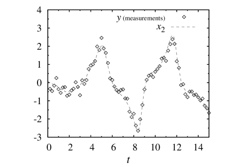
Figure 1: Measurement data. Although a trajectory of $\bm{x}(t)$ is simulated using Eq. (1), the measurement is only performed for $x_{2}$ with the discrete time interval $\Delta\tau^{\mathrm{obs}}=0.2$. In addition, each measurement includes measurement noise (the variance $R=0.04$). We also depict the original trajectory for $x_{2}$ as the dashed line.

The discrete version of the model Eq. (1) has been used in Ref. Lakshmivarahan2009 , and hence we here employ the following parameters, which are similar to the previous work: $\epsilon=1.0$, $Q_{11}=0.0262$, $Q_{22}=0.008$, and $R=0.04$. (Compared with the work in Ref. Lakshmivarahan2009 , we use a little larger measurement noise.) Using these parameters, the data for the estimation problem is created as follows.

Firstly, the time-evolution in Eq. (1) is simulated using the first-order Euler-Maruyama scheme Kloeden_book ; Gardinar_book ; the time interval for the simulation is $10^{-4}$, and the initial conditions are $x_{1}(0)=0.2$ and $x_{2}(0)=0.1$. Secondly, after the simulation of the state variable $\bm{x}(t)$, the measurement procedure is performed; only the state variable $x_{2}$ is extracted, and the measurement noises are added. The time interval for the measurements is $\Delta\tau^{\mathrm{obs}}=0.2$. Finally, we obtain the measurement data depicted in Fig. 1.

The aim of the problem here is to estimate the state variable $\bm{x}(t)$ (i.e., not only $x_{2}(t)$, but also $x_{1}(t)$) from the partially measured data in Fig. 1. Although it is necessary to estimate the covariance matrix $Q$ for the noise in the model and the variance $R$ of the measurement noise in practice, in the present paper, we assume that these parameters are previously known for simplicity.

III Brief review of EnKF

The most famous method for adaptive estimation of the hidden states is the Kalman filter (as for this topic, for example, see Refs. Haykin_book ; Candy_book .) The original Kalman filter was formulated for linear systems under Gaussian noise, and its nonlinear extensions have been studied well. The extensions include the extended Kalman filter, the particle filter, and the EnKF; for the details of these filters, for example, see Ref. Candy_book .

The aim of the present paper is to demonstrate the applicability of the duality concepts. Hence, a new numerical method for the filtering problem, which is based on the duality concepts, will be proposed and discussed later. As a method for comparison, we here employ the EnKF Evensen1994 ; Gillijns2006 ; Evensen2009 because the new method, which will be introduced in Sec.IV, is based on the EnKF. Hence, we here briefly explain the EnKF.

The EnKF uses the Monte Carlo simulations; using an ensemble of many particles, statistical quantities such as means and covariances are evaluated, and these quantities are employed to calculate an important quantity, so-called Kalman gain. Note that we here use the problem settings in Sec. II, and hence the measurements are performed only for the discrete times $\{\tau_{1},\tau_{2},\cdots\}$.

Algorithm for the EnKF

1. Initialization:
   Make the initial ensemble. Here, we choose $n$ samples from a Gaussian distribution with mean $\overline{\bm{x}}(0)$ and covariance matrix $P(0)$, where $\overline{\bm{x}}(0)$ and $P(0)$ are chosen arbitrarily. We denote each sample at time $\tau_{0}=0$ as $\bm{x}_{i}(\tau_{0})$ for $i=1,2,\cdots,n$.

2. Forecast step ($\bm{x}_{i}(\tau_{k-1})\to\bm{x}^{\mathrm{f}}_{i}(\tau_{k})$):
   Using the time-evolution of Eq. (1), simulate the path of the state variable for each sample starting from $\bm{x}_{i}(\tau_{k-1})$. For the simulation, for example, the first-order Euler-Maruyama scheme is available. The simulated path for sample $i$ is denoted as $\bm{x}^{\mathrm{f}}_{i}(t)$ ($\tau_{k-1}<t\leq\tau_{k}$).

3. Assimilation step ($\bm{x}^{\mathrm{f}}_{i}(\tau_{k})\to\bm{x}_{i}(\tau_{k})$):

   1. Make realizations of random variables $\{v_{i}(\tau_{k})\}_{i=1}^{n}$ as the measurement noises. Each realization is obtained from the zero-mean white Gaussian noise with the variance $R$.

   2. Calculate following quantities:
      (mean evaluated from the ensemble)

      $$\overline{\bm{x}}^{\mathrm{f}}(\tau_{k})=\frac{1}{n}\sum_{i=1}^{n}\bm{x}^{\mathrm{f}}_{i}(\tau_{k}),$$ (3)

      (error matrix $E^{\mathrm{f}}(\tau_{k})\in\mathbb{R}^{2\times n}$)

      $$E^{\mathrm{f}}(\tau_{k})$$

      $$=[\bm{x}^{\mathrm{f}}_{1}(\tau_{k})-\overline{\bm{x}}^{\mathrm{f}}(\tau_{k})\quad\cdots\quad\bm{x}^{\mathrm{f}}_{n}(\tau_{k})-\overline{\bm{x}}^{\mathrm{f}}(\tau_{k})],$$ (4)

      (unbiased covariance evaluated from the ensemble)

      $$\widehat{P}^{\mathrm{f}}(\tau_{k})=\frac{1}{n-1}E^{\mathrm{f}}(\tau_{k})(E^{\mathrm{f}}(\tau_{k}))^{\mathrm{T}},$$ (5)

      (mean of the measurement noises)

      $$\overline{v}(\tau_{k})=\frac{1}{n}\sum_{i=1}^{n}v_{i}(\tau_{k}),$$ (6)

      (unbiased variance of the measurement noise)

      $$\widehat{R}(\tau_{k})=\frac{1}{n-1}\sum_{i=1}^{n}\left(v_{i}(\tau_{k})-\overline{v}(\tau_{k})\right)^{2},$$ (7)

      (Kalman gain)

      $$\widehat{K}(\tau_{k})=\widehat{P}^{\mathrm{f}}(\tau_{k})H^{\mathrm{T}}\left(H\widehat{P}^{\mathrm{f}}(\tau_{k})H^{\mathrm{T}}+\widehat{R}(\tau_{k})\right)^{-1}.$$ (8)

   3. Modify the forecasted state variables $\{\bm{x}^{\mathrm{f}}_{i}(\tau_{k})\}_{i=1}^{n}$ using the measurement at time $\tau_{k}$, i.e., $y(\tau_{k})$, as follows:

      $$\bm{x}_{i}(\tau_{k})=\bm{x}^{\mathrm{f}}_{i}(\tau_{k})+\widehat{K}(\tau_{k})\left(y(\tau_{k})+v_{i}(\tau_{k})-H\bm{x}^{\mathrm{f}}_{i}(\tau_{k})\right).$$ (9)

Steps 2 and 3 in the above algorithm are performed for each measurement time step.

In the EnKF, the time evolution in the forecast step is performed as the nonlinear systems, which gives the non-Gaussian distribution for $\{\bm{x}_{i}(t)\}_{i=1}^{n}$ even if we start from a Gaussian distribution. After the time evolution, at each assimilation step, the conventional Kalman filter is employed, which means a filter at least up to the second moment. The final filtered value of the state variable $\bm{x}(t)$ is obtained as the mean of the ensemble $\{\bm{x}_{i}(t)\}_{i=1}^{n}$. In addition, the estimated error could be obtained from the (co)variance of the ensemble $\{\bm{x}_{i}(t)\}_{i=1}^{n}$.

One of the problem in the EnKF is as follows: in order to obtain more accurate estimation results, we need large ensemble size $n$. That is, a small ensemble size gives an inaccurate Kalman gain, and hence the estimation results would not be accurate. In general, it is easy to imagine that the large ensemble size needs high computational costs. Although it has been clarified that a small ensemble size is often enough for the EnKF in practical cases Lakshmivarahan2009 , it would be preferable if we could avoid the numerical simulations of the time evolution of the ensemble at each measurement time step.

IV Algorithm based on duality relations

IV.1 Basic concept

Here, a simple explanation for the basic concept of the duality relation is given; we consider here the duality relation between a stochastic differential equation and a birth-death process. For simplicity, stochastic processes with only one random variable are considered in this subsection.

Suppose that $(x_{t})_{t\geq 0}\in\mathbb{R}$ is a sample trajectory of the stochastic differential equation, and $p(x,t)$ is the probability density at time $t$. It has been known that some stochastic differential equations have the corresponding dual birth-death processes. Denote a dual birth-death process as $(n_{t})_{t\geq 0}\in\mathbb{N}$, whose probability distribution at time $t$ is $P(n,t)$, and then the following equality is satisfied Liggett_book ; Giardina2009 ; Ohkubo2010 ; Ohkubo2013b :

$$\mathbb{E}_{x}\left[x_{t}^{n_{0}}\right]=\mathbb{E}_{n}\left[x_{0}^{n_{t}}\right],$$ (10)

where $\mathbb{E}_{x}$ and $\mathbb{E}_{n}$ are the expectations in the stochastic differential equation $(x_{t})_{t\geq 0}$ starting from $x_{0}$ and in the birth-death process $(n_{t})_{t\geq 0}$ starting from $n_{0}$, respectively. More explicitly, we can rewrite Eq. (10) as

$$\int_{-\infty}^{\infty}p(x,t)x^{n_{0}}dx=\sum_{n=0}^{\infty}P(n,t)x_{0}^{n},$$ (11)

where $p(x,0)=\delta(x-x_{0})$ and $P(n,0)=\delta_{n,n_{0}}$.

Equation (10) shows that the information about the stochastic differential equation can be obtained from the solution of the birth-death process. That is, when we obtain the probability distribution of the birth-death process, $P(n,t)$, with the initial condition $n_{0}=1$, it is possible to evaluate the first order moment, i.e., the mean value of $x_{t}$, of the stochastic differential equation, without solving the stochastic differential equation.

There are several advantages of the usage of the duality relations. It is sometimes easier to treat the birth-death process, compared with the stochastic processes. For some specific cases, the analytical solution of the birth-death process has been obtained. In addition, there are numerical algorithms to simulate the birth-death process efficiently. As for numerical evaluations of the stochastic differential equations, we need some approximation; for example, the time-discretization is needed in the Euler-Maruyama scheme. On the other hand, for example, the Gillespie algorithm for the birth-death process does not need the time-discretization Gillespie1977 . In this sense, the birth-death process would be more tractable than the stochastic differential equations.

Furthermore, only ‘a’ solution of the birth-death process can be used to obtain the information about the stochastic differential equations with ‘arbitrary’ initial conditions. That is, if $n_{0}=1$, $\mathbb{E}_{x}[x_{t}]=\mathbb{E}_{n}[x_{0}^{n_{t}}]=\sum_{n=0}^{\infty}P(n,t)x_{0}^{n}$, and $P(n,t)$ is independent of the value of $x_{0}$. Hence, using only a solution of the birth-death process, $P(n,t)$, it is possible to estimate the average of $x_{t}$, $\mathbb{E}_{x}[x_{t}]$, for the stochastic differential equations for ‘arbitrary’ initial conditions $x_{0}$. Of course, if we want to know the first and second moments of $x_{t}$ in Eq. (10), two solutions of the birth-death process $n_{t}$ with the different initial conditions, $n_{0}=1$ and $n_{0}=2$, are needed. However, once we have these two solutions of the birth-death process, the first and second moments, $\mathbb{E}_{x}[x_{t}]$ and $\mathbb{E}_{x}[x_{t}^{2}]$, with arbitrary initial conditions can be evaluated by using the duality relation in Eq. (10). In contrast, when these moments are evaluated from the direct simulation of the stochastic differential equation, we need many sample trajectories with an initial condition $x_{0}$; if the initial condition $x_{0}$ is changed, we must perform many other numerical simulations.

The basic idea for a new algorithm is as follows; the Monte Carlo simulation in the forecast step in the EnKF is replaced with the simple numerical evaluation based on the duality relation.

The remaining problem is as follows: How should we derive the dual birth-death process from a given stochastic differential equation? In the successive subsections, we will show the method to obtain the dual birth-death process, employing a mathematical formalism called the Doi-Peliti formalism Doi1976a ; Doi1976b ; Peliti1985 ; Tauber2005 .

IV.2 Doi-Peliti formalism

We here briefly review the Doi-Peliti formalism, which is useful to obtain the duality relations. The Doi-Peliti formalism is the method similar to the second quantization method in quantum mechanics. Up to now, the Doi-Peliti formalism has been used in various contexts, mainly in order to investigate discrete systems such as chemical reactions, and it has been shown that the algebraic probability theory Hora_book gives the mathematical basis of the Doi-Peliti formalism Ohkubo2013a .

In the Doi-Peliti formalism, creation operator $a^{\dagger}$ and annihilation operator $a$ are introduced, which satisfy the following commutation relation:

$$[a,a^{\dagger}]\equiv aa^{\dagger}-a^{\dagger}a=1,\quad[a,a]=[a^{\dagger},a^{\dagger}]=0.$$ (12)

These operators act on a vector in the Fock space, $|n\rangle$, as follows:

$$a^{\dagger}|n\rangle=|n+1\rangle,\quad a|n\rangle=n|n-1\rangle,$$ (13)

and the vacuum state $|0\rangle$ is characterized by $a|0\rangle=0$. Additionally, vectors $\{\langle m|\}_{m=0}^{\infty}$ satisfy the following orthogonal relation to the vectors $\{|n\rangle\}_{n=0}^{\infty}$:

$$\langle m|n\rangle=\delta_{m,n}n!.$$ (14)

Note that $a^{\dagger}a$ corresponds to the number operator and

$$a^{\dagger}a|n\rangle=n|n\rangle.$$ (15)

It has been shown that the Doi-Peliti formalism is deeply related to the conventional generating function method Droz1994 , and the following correspondences can be useful to understand the usage of the Doi-Peliti formalism in the duality problem:

$$|n\rangle\leftrightarrow x^{n},\quad a^{\dagger}\leftrightarrow x,\quad a\leftrightarrow\frac{\partial}{\partial x}.$$ (16)

That is, the differential operator is connected to the annihilation operator, which is used in partial differential equations derived from stochastic differential equations. In addition, the annihilation operator acts on the discrete states $|n\rangle$, which is available to construct the birth-death process, as shown later. The important point here is that the Doi-Peliti formalism can bridge continuous states with discrete states, which corresponds to the connection between a stochastic differential equation and a birth-death process.

IV.3 Derivation of the dual birth-death process

The derivation of the simple duality relation, such as Eq. (10), has been discussed in Ref. Giardina2009 , and the derivation based on the Doi-Peliti formalism has also been proposed Ohkubo2010 . However, in order to treat the estimation problem, only the simple duality relation in Eq. (10) is not enough; the simple duality relation in Eq. (10) can deal with only a very restricted class of stochastic differential equations. Recently, extended duality relations have been proposed Ohkubo2013b , which is necessary to construct the new algorithm based on the duality relation. Here, we only show, as an example, the derivation of a dual birth-death process from the stochastic differential equations in Eq. (1). For the mathematical details, see the original paper Ohkubo2013b .

First of all, it is needed to construct the corresponding Fokker-Planck equation of the stochastic differential equations in Eq. (1). (For the derivation of the Fokker-Planck equation from the stochastic differential equations, see, for example, Ref. Gardinar_book .) The corresponding Fokker-Planck equation is as follows:

$$\frac{\partial}{\partial t}p(x_{1},x_{2},t)$$

$$=\left[-\frac{\partial}{\partial x_{1}}x_{2}-\frac{\partial}{\partial x_{2}}\left[\epsilon(1-x_{1}^{2})x_{2}-x_{1}\right]\right]p(x_{1},x_{2},t)$$

$$\quad+\frac{1}{2}\left[Q_{11}\frac{\partial^{2}}{\partial x_{1}^{2}}+Q_{22}\frac{\partial^{2}}{\partial x_{2}^{2}}\right]p(x_{1},x_{2},t),$$ (17)

where $p(x_{1},x_{2},t)$ is the probability density at time $t$ for the stochastic differential equations. For notational convenience, we introduce the following linear operator $L^{*}$:

$$L^{*}\left(x_{1},\frac{\partial}{\partial x_{1}},x_{2},\frac{\partial}{\partial x_{2}}\right)$$

$$=\left[-\frac{\partial}{\partial x_{1}}x_{2}-\frac{\partial}{\partial x_{2}}\left[\epsilon(1-x_{1}^{2})x_{2}-x_{1}\right]\right]$$

$$\quad+\frac{1}{2}\left[Q_{11}\frac{\partial^{2}}{\partial x_{1}^{2}}+Q_{22}\frac{\partial^{2}}{\partial x_{2}^{2}}\right],$$ (18)

and hence the Fokker-Planck equation  (17) is rewritten as

$$\frac{\partial}{\partial t}p(x_{1},x_{2},t)=L^{*}\left(x_{1},\frac{\partial}{\partial x_{1}},x_{2},\frac{\partial}{\partial x_{2}}\right)p(x_{1},x_{2},t).$$ (19)

The adjoint operator of Eq. (18), $L$, is as follows:

$$L\left(x_{1},\frac{\partial}{\partial x_{1}},x_{2},\frac{\partial}{\partial x_{2}}\right)$$

$$=x_{2}\frac{\partial}{\partial x_{1}}-\epsilon(1-x_{1}^{2})x_{2}\frac{\partial}{\partial x_{2}}-x_{1}\frac{\partial}{\partial x_{2}}$$

$$\quad+\frac{1}{2}\left[Q_{11}\frac{\partial^{2}}{\partial x_{1}^{2}}+Q_{22}\frac{\partial^{2}}{\partial x_{2}^{2}}\right],$$ (20)

and using the correspondence between operators in the Doi-Peliti formalism and the differential operators in Eq. (16), we have

$$L\left(a^{\dagger}_{1},a_{1},a^{\dagger}_{2},a_{2}\right)$$

$$=a^{\dagger}_{2}a_{1}+\epsilon(1-a^{\dagger}_{1}a^{\dagger}_{1})a^{\dagger}_{2}a_{2}-a^{\dagger}_{1}a_{2}$$

$$\quad+\frac{1}{2}\left[Q_{11}a_{1}a_{1}+Q_{22}a_{2}a_{2}\right],$$ (21)

where the following correspondences are used:

$$a_{1}^{\dagger}\leftrightarrow x_{1},\quad a_{1}\leftrightarrow\frac{\partial}{\partial x_{1}},\quad a_{2}^{\dagger}\leftrightarrow x_{2},\quad a_{2}\leftrightarrow\frac{\partial}{\partial x_{2}}.$$ (22)

In addition, as discussed later, it is convenient to introduce the time scaling $t=r_{\mathrm{ts}}\tilde{t}$; due to the time scaling, the original Fokker-Planck equation  (19) is rewritten as

$$\frac{\partial}{\partial\tilde{t}}p(x_{1},x_{2},r_{\mathrm{ts}}\tilde{t})$$

$$=r_{\mathrm{ts}}L^{*}\left(x_{1},\frac{\partial}{\partial x_{1}},x_{2},\frac{\partial}{\partial x_{2}}\right)p(x_{1},x_{2},r_{\mathrm{ts}}\tilde{t}).$$ (23)

We here focus on the fact that continuous variables, $x_{1}$ and $x_{2}$, are replaced with creation operators in Eq. (22). Hence, if we reinterpret a constant as a creation operator, the following replacement is available:

$$r_{\mathrm{ts}}\leftrightarrow a^{\dagger}_{0},$$ (24)

and therefore the following linear operator is obtained:

$$L\left(a^{\dagger}_{0},a^{\dagger}_{1},a_{1},a^{\dagger}_{2},a_{2}\right)$$

$$\equiv a^{\dagger}_{0}L\left(a^{\dagger}_{1},a_{1},a^{\dagger}_{2},a_{2}\right)$$

$$=a^{\dagger}_{0}a^{\dagger}_{2}a_{1}+\epsilon a^{\dagger}_{0}a^{\dagger}_{2}a_{2}-\epsilon a^{\dagger}_{0}(a^{\dagger}_{1})^{2}a^{\dagger}_{2}a_{2}-a^{\dagger}_{0}a^{\dagger}_{1}a_{2}$$

$$\quad+\frac{1}{2}\left[Q_{11}a^{\dagger}_{0}a_{1}a_{1}+Q_{22}a^{\dagger}_{0}a_{2}a_{2}\right].$$ (25)

Note that all creation operators in each term in Eq. (25) are placed on the left side of the annihilation operators; if not, we must replace the term using the commutation relation in Eq. (12).

Since the linear operator in Eq. (25) acts on the Fock space, i.e., the discrete state space $\{|n\rangle\}_{n=0}^{\infty}$, one may expect that the linear operator simply gives the time-evolution for a birth-death process. That is, defining the state vector $|\psi(\tilde{t})\rangle$ as

$$|\psi(\tilde{t})\rangle\equiv\sum_{n_{0}=0}^{\infty}\sum_{n_{1}=0}^{\infty}\sum_{n_{2}=0}^{\infty}P(n_{0},n_{1},n_{2},\tilde{t})|n_{0},n_{1},n_{2}\rangle,$$

where $P(n_{0},n_{1},n_{2},\tilde{t})$ is a probability distribution of a birth-death process, and considering the time-evolution equation

$$\frac{\partial}{\partial\tilde{t}}|\psi(\tilde{t})\rangle=L(a_{0}^{\dagger},a_{1}^{\dagger},a_{1},a_{2}^{\dagger},a_{2})|\psi(\tilde{t})\rangle,$$

we may have a time-evolution equation for $P(n_{0},n_{1},n_{2},\tilde{t})$ by comparing the coefficient of a state vector $|n_{0},n_{1},n_{2}\rangle$ on the right and left hand sides. However, as discussed in the previous work Ohkubo2013b , it is impossible to simply interpret the linear operator in Eq. (25) as a time-evolution operator for a birth-death process; the linear operator does not satisfy the probability conservation law, and, in addition, some terms seem to correspond to ‘negative’ transition rates.

In order to construct an adequate birth-death process, we need an additional operator $b$, which satisfies the following relations:

$$b|+\rangle=|-\rangle,\quad b|-\rangle=|+\rangle,$$ (26)

where $|+\rangle$ and $|-\rangle$ are orthonormal state vectors satisfying $\langle+|+\rangle=\langle-|-\rangle=1$ and $\langle+|-\rangle=\langle-|+\rangle=0$. The following procedure is needed to construct an adequate time-evolution operator for a birth-death process (although the following procedure might seem complicated, a concrete example will be given soon):

1. For each term in the linear operator $L$, apply the following procedures.

2. If the coefficient of the term has a negative sign, replace the negative sign ‘$-$’ with ‘$+b$’ using the operator $b$.

3. Act the operators on $|\bm{n}\rangle$, and evaluate the coefficient including the effects of the number operators $a^{\dagger}_{i}a_{i}$.

4. Subtract a term in order to guarantee the probability conservation law; the term gives the same coefficient with Step 2, and additionally, the term consists of the same number of creation and annihilation operators for the same sub-index.

5. In order to compensate the subtracted term, add the same term with Step 3.

For example, the first term in Eq. (25) is $a^{\dagger}_{0}a^{\dagger}_{2}a_{1}$, and then we do not need Step 1. Since

$$a^{\dagger}_{0}a^{\dagger}_{2}a_{1}|n_{0},n_{1},n_{2}\rangle=n_{1}|n_{0}+1,n_{1}-1,n_{2}+1\rangle,$$ (27)

the coefficient is $n_{1}$, and therefore the term $a^{\dagger}_{1}a_{1}$ must be subtracted in Step 2. On the other hand, the third term in Eq. (25), $-\epsilon a^{\dagger}_{0}(a^{\dagger}_{1})^{2}a^{\dagger}_{2}a_{2}$, has the negative sign, and hence Step 1 gives $+b\epsilon a^{\dagger}_{0}(a^{\dagger}_{1})^{2}a^{\dagger}_{2}a_{2}$. The subtracted term in Step 3 is $b\epsilon a^{\dagger}_{2}a_{2}$ because

$$a^{\dagger}_{0}(a^{\dagger}_{1})^{2}a^{\dagger}_{2}a_{2}|n_{0},n_{1},n_{2}\rangle=n_{2}|n_{0}+1,n_{1}+2,n_{2}\rangle,$$ (28)

which gives the coefficient $n_{2}$.

Using the above procedure, we obtain the following linear operator, instead of the linear operator $L$ in Eq. (25):

$$L\left(a^{\dagger}_{0},a_{0},a^{\dagger}_{1},a_{1},a^{\dagger}_{2},a_{2},b\right)$$

$$=L^{\prime}\left(a^{\dagger}_{0},a_{0},a^{\dagger}_{1},a_{1},a^{\dagger}_{2},a_{2},b\right)+V\left(a^{\dagger}_{1}a_{1},a^{\dagger}_{2}a_{2}\right),$$ (29)

where

$$L^{\prime}\left(a^{\dagger}_{0},a_{0},a^{\dagger}_{1},a_{1},a^{\dagger}_{2},a_{2},b\right)$$

$$=(a^{\dagger}_{0}a^{\dagger}_{2}a_{1}-a^{\dagger}_{1}a_{1})+(\epsilon a^{\dagger}_{0}a^{\dagger}_{2}a_{2}-\epsilon a^{\dagger}_{2}a_{2})$$

$$\quad+(\epsilon ba^{\dagger}_{0}(a^{\dagger}_{1})^{2}a^{\dagger}_{2}a_{2}-\epsilon a^{\dagger}_{2}a_{2})+(ba^{\dagger}_{0}a^{\dagger}_{1}a_{2}-a^{\dagger}_{2}a_{2})$$

$$\quad+\left(\frac{1}{2}Q_{11}a^{\dagger}_{0}a_{1}a_{1}-\frac{1}{2}Q_{11}a^{\dagger}_{1}a^{\dagger}_{1}a_{1}a_{1}\right)$$

$$\quad+\left(\frac{1}{2}Q_{22}a^{\dagger}_{0}a_{2}a_{2}-\frac{1}{2}Q_{22}a^{\dagger}_{2}a^{\dagger}_{2}a_{2}a_{2}\right)$$ (30)

and

$$V\left(a^{\dagger}_{1}a_{1},a^{\dagger}_{2}a_{2}\right)$$

$$=a^{\dagger}_{1}a_{1}+2\epsilon a^{\dagger}_{2}a_{2}+a^{\dagger}_{2}a_{2}+\frac{1}{2}Q_{11}\left((a^{\dagger}_{1}a_{1})(a^{\dagger}_{1}a_{1})-a^{\dagger}_{1}a_{1}\right)$$

$$\quad+\frac{1}{2}Q_{22}\left((a^{\dagger}_{2}a_{2})(a^{\dagger}_{2}a_{2})-a^{\dagger}_{2}a_{2}\right).$$ (31)

Note that we used $a^{\dagger}a^{\dagger}aa=(a^{\dagger}a)(a^{\dagger}a)-aa$, which stems from $[a,a^{\dagger}]=aa^{\dagger}-a^{\dagger}a=1$.

As shown in the previous work Ohkubo2013b , it is possible to interpret the linear operator $L^{\prime}$ in Eq. (30) as a time-evolution operator for a birth-death process. Because of the operator $b$, we must consider an additional state variable, which takes only two states ($+$ or $-$), in addition to the state variables $n_{0},n_{1}$ and $n_{2}$. See the first term in Eq. (30); the action of the first term on $|\bm{n}\rangle$ is Eq. (27), and hence we can interpret this term as an elementary birth-death process $X_{1}\to X_{2}+X_{0}$ with rate $n_{1}$, where $n_{0},n_{1}$ and $n_{2}$ is the number of particles $X_{0},X_{1}$, and $X_{2}$, respectively. On the other hand, the third term in Eq. (30) gives $X_{2}\to 2X_{1}+X_{2}+X_{0}$ and the state change with $+\to-$ or $-\to+$ with rate $\epsilon n_{2}$; the state ($+$ or $-$) is changed due to an event corresponding to the third term. Repeating the similar discussions, finally the following birth-death process is obtained:

$$\begin{cases}\mathrm{(i)}&X_{1}\xrightarrow{n_{1}}X_{2}+X_{0},\\ \mathrm{(ii)}&X_{2}\xrightarrow{\epsilon n_{2}}X_{2}+X_{0},\\ \mathrm{(iii)}&X_{2}\xrightarrow{\epsilon n_{2}}2X_{1}+X_{2}+X_{0}\quad\textrm{with S.C.},\\ \mathrm{(iv)}&X_{2}\xrightarrow{n_{2}}X_{1}+X_{0}\quad\textrm{with S.C.},\\ \mathrm{(v)}&2X_{1}\xrightarrow{n_{1}(n_{1}-1)}X_{0},\\ \mathrm{(vi)}&2X_{2}\xrightarrow{n_{2}(n_{2}-1)}X_{0},\end{cases}$$ (32)

where ‘S.C.’ means the state change $+\to-$ or $-\to+$.

The term $V(a^{\dagger}_{1}a_{1},a^{\dagger}_{2}a_{2})$ is called a Feynman-Kac term, and the important point is that this term is written only in terms of the number operators $a^{\dagger}_{i}a_{i}$. Since the number operators $a^{\dagger}_{i}a_{i}$ does not affect the state vectors, we can simply replace the number operators with the random variables in the birth-death process; i.e., $V(a^{\dagger}_{1}a_{1},a^{\dagger}_{2}a_{2})=V(n_{1},n_{2})$.

The intuitive understanding of the duality relation is written as follows: we here abbreviate a state related to the Fokker-Plank equation at time $t$ as $\mathrm{FP}(t)$ and that to the birth-death process as $\mathrm{BD}(t)$. In addition, for simplicity, set $r_{\mathrm{ts}}=1$ and hence $t=\tilde{t}$; furthermore, we neglect the Feynman-Kac term here. Then, formally, time-evolution of $\mathrm{BD}(t)$ is given by $\mathrm{BD}(t)=e^{Lt}\mathrm{BD}(0)$. In contrast, that of $\mathrm{FP}(t)$ is written as $\mathrm{FP}(t)=\mathrm{FP}(0)e^{Lt}$, when we consider the left-action of $L$. Hence, the adjoint operator $L^{*}$ gives the actual time-evolution of the Fokker-Planck equation. In addition, we have formally $\mathrm{FP}(t)\mathrm{BD}(0)=\mathrm{FP}(0)e^{Lt}\mathrm{BD}(0)=\mathrm{FP}(0)\mathrm{BD}(t)$; this corresponds to the duality relation. The linear operator $L$ can be written in terms of both the differential operators and the creation-annihilation operators, and hence the stochastic differential equation in Eq. (1) and the birth-death process in Eq. (32) are connected naturally. Of course, the above discussion is just an intuitive one, and for the mathematical explanation of the duality relations, see the previous work Ohkubo2013b .

Here we consider a time-evolution from time $0$ to $\tau$. Because we consider the time-scaling factor $r_{\mathrm{ts}}$, the time interval, $\tau$, in the stochastic differential equations correspond to the time interval $\tilde{\tau}=\tau/r_{\mathrm{ts}}$ in the dual birth-death process. Using the duality relation, we can obtain the following identity:

$$\mathbb{E}_{\bm{x}}\left[x_{1}(\tau)^{n_{1}(0)}x_{2}(\tau)^{n_{2}(0)}\right]$$

$$=\mathbb{E}_{\bm{n},+}\Bigg{[}\exp\left\{\int_{0}^{\tilde{\tau}}V(n_{1}(s),n_{2}(s))ds\right\}r_{\mathrm{ts}}^{n_{0}(\tilde{\tau})}x_{1}(0)^{n_{1}(\tilde{\tau})}x_{2}(0)^{n_{2}(\tilde{\tau})}\Bigg{]}$$

$$\,\,-\mathbb{E}_{\bm{n},-}\Bigg{[}\exp\left\{\int_{0}^{\tilde{\tau}}V(n_{1}(s),n_{2}(s))ds\right\}r_{\mathrm{ts}}^{n_{0}(\tilde{\tau})}x_{1}(0)^{n_{1}(\tilde{\tau})}x_{2}(0)^{n_{2}(\tilde{\tau})}\Bigg{]},$$ (33)

where the abbreviations $\bm{x}=(x_{1},x_{2})$ and $\bm{n}=(n_{0},n_{1},n_{2})$ are used; we set $n_{0}(0)=0$; $\mathbb{E}_{\bm{n},+}$ and $\mathbb{E}_{\bm{n},-}$ are the expectations related to the states $+$ and $-$ in the birth-death process in Eq. (32), respectively. Using the duality relation in Eq. (33), we can evaluate various information for the stochastic differential equation in Eq. (1) from the solution of the birth-death process in Eq. (32). In order to evaluate the probability distribution and the corresponding Feynman-Kac terms for the birth-death process in Eq. (32), Monte Carlo simulations with the Gillespie algorithm are available.

As noted in Sec. IV.A, the initial conditions for the birth-death process correspond to the order of moments in the stochastic differential equation. When we use $n_{1}(0)=2$ and $n_{2}(0)=0$, the time-evolution of the second moment for $x_{1}$, i.e., $\mathbb{E}_{\bm{x}}[x_{1}(\tau)^{2}]$, is evaluated.

Using the above procedures, the time evolution of the stochastic differential equation for arbitrary initial conditions can be replaced with that of the dual birth-death process for specific initial conditions. In addition, if changing the time-scaling variable $r_{\mathrm{ts}}$, we can evaluate information for various time interval in the stochastic differential equations from only a result for a single fixed time interval $\tilde{\tau}$ in the birth-death process. For example, assume that $\tilde{\tau}=1$; if we want to know the information of the stochastic differential equation at time $t=1$, we should set $r_{\mathrm{ts}}=1$. On the other hand, the information at time $t=0.9$ can be evaluated from the same results of the birth-death process with $\tilde{\tau}=1$ and setting $r_{\mathrm{ts}}=0.9$. Hence, there is no need to perform the Monte Carlo simulations for various different time intervals; this is also one of the advantages of the new method.

At the end of this subsection, we give one comment for the operator $b$. In the above construction, we replaced the minus sign ‘$-$’ with the operator ‘$+b$’ and avoided the ‘negative’ transition problem. Instead of that, we can use the following trick: Interpret constants as random variables. That is, we interpret ‘$-1$’ as a random variable $x_{3}$, and the (stochastic) differential equation for $x_{3}$ is set as $\displaystyle dx_{3}/dt=0$. Then, employing the same discussion above, $x_{3}$ is replaced with $a_{3}^{\dagger}$ in the Doi-Peliti formulation, and finally we obtain the following birth-death process

$$\begin{cases}\mathrm{(i)}&X_{1}\xrightarrow{n_{1}}X_{2}+X_{0},\\ \mathrm{(ii)}&X_{2}\xrightarrow{\epsilon n_{2}}X_{2}+X_{0},\\ \mathrm{(iii)}&X_{2}\xrightarrow{\epsilon n_{2}}2X_{1}+X_{2}+X_{0}+X_{3},\\ \mathrm{(iv)}&X_{2}\xrightarrow{n_{2}}X_{1}+X_{0}+X_{3},\\ \mathrm{(v)}&2X_{1}\xrightarrow{n_{1}(n_{1}-1)}X_{0},\\ \mathrm{(vi)}&2X_{2}\xrightarrow{n_{2}(n_{2}-1)}X_{0},\end{cases}$$ (34)

and the following duality relation

$$\mathbb{E}_{\bm{x}}\left[x_{1}(\tau)^{n_{1}(0)}x_{2}(\tau)^{n_{2}(0)}x_{3}(\tau)^{n_{3}(0)}\right]$$

$$=\mathbb{E}_{\bm{n}}\Bigg{[}\exp\left\{\int_{0}^{\tilde{\tau}}V(n_{1}(s),n_{2}(s))ds\right\}$$

$$\qquad\quad\times r_{\mathrm{ts}}^{n_{0}(\tilde{\tau})}x_{1}(0)^{n_{1}(\tilde{\tau})}x_{2}(0)^{n_{2}(\tilde{\tau})}x_{3}(0)^{n_{2}(\tilde{\tau})}\Bigg{]},$$ (35)

where the abbreviations $\bm{x}=(x_{1},x_{2},x_{3})$ and $\bm{n}=(n_{0},n_{1},n_{2},n_{3})$ are used. Note that the Feynman-Kac term does not depend on $n_{3}(t)$. Because the ‘random’ variable $x_{3}(t)$ is a time-independent constant and $x_{3}(t)\equiv-1$, we can see that the initial condition, $n_{0}(0)=0$ and $n_{3}(0)=0$, recovers the original duality relation in Eq. (33). This technique, in which constants are interpreted as random variables, would be sometimes useful to consider more complicated stochastic differential equations. However, in the example considered here, only the ‘negative’ transition rate should be avoided, and the expression in Eq. (33) is simpler in computational viewpoint; although $n_{3}(t)$ takes any natural numbers, the additional states $|+\rangle$ and $|-\rangle$ takes only two states, and hence the computational memory in Monte Carlo simulations is largely reduced. From this reason, the additional operator $b$ is introduced and used in the present paper.

IV.4 Moment evaluation

The duality relation in Eq. (33) can be used for evaluating the moments in stochastic differential equation in Eq. (1) starting from the Dirac-delta-type initial conditions, as discussed in Sec. IV.A. However, in the EnKF, we use an ensemble of samples. In the EnKF, only the mean and covariance matrix of the ensemble are needed, so we can consider that the ensemble is essentially characterized by a Gaussian distribution. Hence, the Dirac-delta-type initial conditions are not enough.

We here write the expectation value, which is taken by using a Gaussian distribution with mean $\bm{x}(t)$ and covariance matrix $V$, as $\langle\cdots\rangle$. Hence, the first term in the r.h.s. in Eq. (33) should be replaced with

$$\left\langle\mathbb{E}_{\bm{n},+}\left[e^{\int_{0}^{\tilde{\tau}}Vds}r_{\mathrm{ts}}^{n_{0}(\tilde{\tau})}x_{1}(0)^{n_{1}(\tilde{\tau})}x_{2}(0)^{n_{2}(\tilde{\tau})}\right]\right\rangle$$

$$=\mathbb{E}_{\bm{n},+}\left[e^{\int_{0}^{\tilde{\tau}}Vds}r_{\mathrm{ts}}^{n_{0}(\tilde{\tau})}\left\langle x_{1}(0)^{n_{1}(\tilde{\tau})}x_{2}(0)^{n_{2}(\tilde{\tau})}\right\rangle\right].$$

We need a little additional calculations in order to evaluate the expectation with the Gaussian distribution; introducing the following notations,

$$\mu_{1}=\langle x_{1}\rangle,\mu_{2}=\langle x_{2}\rangle,$$ (36)

the following recursion formula is known Willink2005 :

$$\left\langle x_{1}^{n_{1}}x_{2}^{n_{2}}\right\rangle= \mu_{1}\left\langle x_{1}^{n_{1}-1}x_{2}^{n_{2}}\right\rangle+V_{11}(n_{1}-1)\left\langle x_{1}^{n_{1}-2}x_{2}^{n_{2}}\right\rangle$$

$$+V_{12}n_{2}\left\langle x_{1}^{n_{1}-1}x_{2}^{n_{2}-1}\right\rangle$$ (37)

or

$$\left\langle x_{1}^{n_{1}}x_{2}^{n_{2}}\right\rangle= \mu_{2}\left\langle x_{1}^{n_{1}}x_{2}^{n_{2}-1}\right\rangle+V_{21}n_{1}\left\langle x_{1}^{n_{1}-1}x_{2}^{n_{2}-1}\right\rangle$$

$$+V_{22}(n_{2}-1)\left\langle x_{1}^{n_{1}}x_{2}^{n_{2}-2}\right\rangle.$$ (38)

Using the above recursion formula, once we have the probability distribution $P(n_{0},n_{1},n_{2},t)$ for the birth-death process in Eq. (32) with adequate initial values, it is possible to evaluate various moments for the stochastic differential equation in Eq. (1) with a Gaussian initial distribution, using the following duality relation:

$$\mathbb{E}_{\bm{x},\textrm{Gaussian initial}}\left[x_{1}(\tau)^{n_{1}(0)}x_{2}(\tau)^{n_{2}(0)}\right]$$

$$=\mathbb{E}_{\bm{n},+}\Bigg{[}\exp\left\{\int_{0}^{\tilde{\tau}}V(n_{1}(s),n_{2}(s))ds\right\}r_{\mathrm{ts}}^{n_{0}(\tilde{\tau})}\left\langle x_{1}(0)^{n_{1}(\tilde{\tau})}x_{2}(0)^{n_{2}(\tilde{\tau})}\right\rangle\Bigg{]}$$

$$\,\,-\mathbb{E}_{\bm{n},-}\Bigg{[}\exp\left\{\int_{0}^{\tilde{\tau}}V(n_{1}(s),n_{2}(s))ds\right\}r_{\mathrm{ts}}^{n_{0}(\tilde{\tau})}\left\langle x_{1}(0)^{n_{1}(\tilde{\tau})}x_{2}(0)^{n_{2}(\tilde{\tau})}\right\rangle\Bigg{]}.$$ (39)

IV.5 Algorithm

We here consider general cases with variable time intervals, and denote the maximum of the time intervals, $\tau_{k-1}-\tau_{k}$, as $\Delta\tau$. The new Kalman filter based on the duality relation, called the DuKF here, is as follows:

Algorithm for DuKF

1. Preparation for the duality relations:
   Simulate the dual birth-death process in Eq. (32). We need simulations with five different initial conditions;

   • $n_{0}=0,n_{1}=1,n_{2}=0$,

   • $n_{0}=0,n_{1}=0,n_{2}=1$,

   • $n_{0}=0,n_{1}=2,n_{2}=0$,

   • $n_{0}=0,n_{1}=0,n_{2}=2$,

   • $n_{0}=0,n_{1}=1,n_{2}=1$,

   which are necessary to evaluate $\mathbb{E}_{\bm{x}}[x_{1}(t)]$, $\mathbb{E}_{\bm{x}}[x_{2}(t)]$, $\mathbb{E}_{\bm{x}}[x_{1}(t)^{2}]$, $\mathbb{E}_{\bm{x}}[x_{2}(t)^{2}]$, $\mathbb{E}_{\bm{x}}[x_{1}(t)x_{2}(t)]$, respectively. For all cases, the additional state variable is set to ‘$+$’ initially. The Monte Carlo simulations are performed from $t=0$ to $t=\Delta\tau$, and the integral of the Feynman-Kac term $V(n_{1},n_{2})$ and the final probability distribution $P(n_{0},n_{1},n_{2},\Delta\tau)$ are evaluated numerically.

2. Initialization:
   Set an initial Gaussian distribution with mean $\overline{\bm{x}}^{\mathrm{a}}(0)$ and covariance matrix $P^{\mathrm{a}}(0)$.

3. Forecast step at $\tau_{k-1}$:
   Using the duality relation in Eq. (39), evaluate various moments, which are necessary to characterize a Gaussian distribution. The ensemble average in Eq. (39), $\langle\cdots\rangle$, is taken for the Gaussian distribution with mean $\overline{\bm{x}}^{\mathrm{a}}(\tau_{k-1})$ and covariance matrix $P^{\mathrm{a}}(\tau_{k-1})$. The above procedure gives the mean $\overline{\bm{x}}^{\mathrm{f}}(\tau_{k})$ and the covariance $\widehat{P}^{\mathrm{f}}(\tau_{k})$ of the nonlinear systems at time $\tau_{k}$. Note that the time-scaling variable $r_{\mathrm{ts}}$ must be selected adequately according to the ratio between $\tau_{k}-\tau_{k-1}$ and $\Delta\tau$.

4. Assimilation step at $\tau_{k}$:
   Calculate the Kalman gain

   $$\widehat{K}(\tau_{k})=\widehat{P}^{\mathrm{f}}(\tau_{k})H^{\mathrm{T}}\left(H\widehat{P}^{\mathrm{f}}(\tau_{k})H^{\mathrm{T}}+R\right)^{-1},$$ (40)

   where $H$ is the matrix assigned for the measurement and $R$ the variance of the measurement; see Eq. (2). Update the following quantities:

   $$\overline{\bm{x}}^{\mathrm{a}}(\tau_{k})=\overline{\bm{x}}^{\mathrm{f}}(\tau_{k})+\widehat{K}(\tau_{k})\left(y(\tau_{k})-H\overline{\bm{x}}^{\mathrm{f}}(\tau_{k})\right)$$ (41)

   and

   $$P^{\mathrm{a}}(\tau_{k})=(1-\widehat{K}(\tau_{k})H)\widehat{P}^{\mathrm{f}}(\tau_{k}).$$ (42)

Steps 3 and 4 are performed for each measurement time step.

V Results

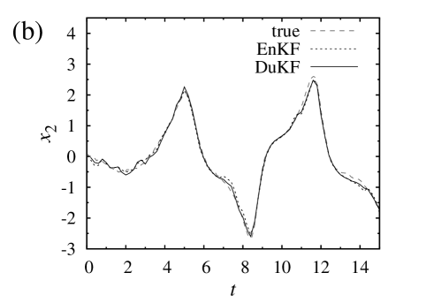
Figure 2: State estimates $x_{1}$ and $x_{2}$ for the stochastic differential equations (1); (a) for the unobserved state variable $x_{1}$, and (b) for the state variable $x_{2}$, which is observed with noise. Note that $x_{2}$ is measured only at discrete times as shown in Fig. 1. For the EnKF, we set $n=10$ and $\Delta t=10^{-4}$ in the Euler-Maruyama scheme.

In order to demonstrate the DuKF, we employ the algorithm in Sec. IV.E to the problem in Sec. II. For simplicity, we assume here that the parameters in the stochastic differential equations, $Q$ and $R$, are previously known, as explained in Sec. II. We use the following parameters for the initial Gaussian distribution; $\overline{\bm{x}}(0)=(0.1,0.1)$, $[P(0)]_{11}=0.1$, $[P(0)]_{12}=[P(0)]_{21}=0$, and $[P(0)]_{22}=0.1$. Firstly, for the DuKF, we performed the Monte Carlo simulations for the dual birth-death process using the Gillespie algorithm Gillespie1977 . For each initial condition, $10^{12}$ sample paths were generated, and the Feynman-Kac term and the probability distribution were evaluated.

Figure 2 shows the results of the state estimation. Note that only the state variable $x_{2}$ is observed at discrete times, as depicted in Fig. 1. Although the observation contains the measurement noises, as seen in Fig. 1, both the EnKF and DuKF give adequate estimations. Especially, the non-observed state $x_{1}$ can be estimated reasonably as shown in Fig. 2. Note that the initial guesses for $\bm{x}$ are not far from the true values, and hence it is difficult to see the initial transient behavior for both the EnKF and DuKF. From Fig. 2, it may be difficult to judge whether the DuKF gives better results than the EnKF or not, but we confirmed that the DuKF gives a slightly better mean squared error. If we want to obtain the similar mean squared error, we need larger ensemble for the EnKF, and the larger ensemble needs more computational time. On the other hands, the forecast step in the DuKF does not need any Monte Carlo simulation, and hence the DuKF works rapidly. Actually, in order to deal with the current data, the EnKF with ensemble size $n=10$ and original discretized time step for simulations ($10^{-4}$) needs about $0.8$ seconds in a standard computer with Intel Core i5 processor (2.2GHz). In contrast, the DuKF needs less than $0.1$ seconds. As shown below, the ensemble size $n=10$ is not enough large, and if we use $n=1000$ ensembles, $1000$ times costs of simulations are needed for the EnKF. (Of course, the DuKF needs pre-calculations for the dual birth-death processes. For $10^{12}$ sample paths, about one month calculations were needed, but we can reuse the pre-calculation results repeatedly in the actual filtering steps.)

Figure 3: Covariance between $x_{1}$ and $x_{2}$, $[P(t)]_{12}$, calculated in the EnKF and DuKF. The evaluated covariance is used to calculate the Kalman gain. The evaluation in the EnKF approaches to that in the DuKF when larger ensembles are used.

In order to see the difference between the EnKF and DuKF more explicitly, we show the covariance $[P(t)]_{12}$ calculated in the EnKF and DuKF in Fig. 3. As shown in Fig. 3, the larger ensemble size in the EnKF gives the similar covariance with that of the DuKF. The covariance is used to evaluate the Kalman gain, and hence more accurate covariance is necessary to have better estimations. The ensemble size of order $10^{3}$ is needed to obtain the similar covariance with that of the DuKF; it is very time-consuming. In addition, it would be needed to choose an adequate time-interval $\Delta t$ for the simulation in the Euler-Maruyama scheme for the stochastic differential equations; the computational time and the precision of the estimations in EnKF largely depend on $\Delta t$. On the other hand, we do not need such time discretization for the DuKF when the Gillespie algorithm is employed, as discussed before.

VI Concluding remarks

The duality relation between stochastic processes has been still developing, and hence it is expected that new applications of the duality relations give completely novel algorithms for various research fields. We demonstrate one of the applications by using the estimation problem. As a result, pre-calculations for the dual birth-death processes enable us to avoid the time-consuming Monte Carlo simulations for each forecast step.

Of course, we do not claim that the proposed DuKF is always superior to the EnKF for any estimation problem. Actually, the implementation of the EnKF is simpler than that of the DuKF. In addition, there could be more appropriate methods for specific tasks (see, for example, Palatella2013 .) In order to make the DuKF more practical, it is needed to develop more efficient numerical methods for the dual birth-death processes; very high accuracy is necessary. Actually, in preliminary works, the famous Lorenz system was investigated, but the DuKF works well only for very short observation time intervals, and then it was not practical. If we have more accurate numerical results, it would be possible to make the DuKF for the chaotic systems. In order to overcome this problem, it may be possible to employ simulations based on the important sampling methods Asmussen_book ; Landau_book . Note that it has not yet been clarified what factors determine the pre-calculation time; the preliminary works for the Lorenz systems could suggest that the chaotic behavior is related to the demands for the high-accuracy of the pre-calculation, but more detailed studies should be done in future from both experimental and theoretical view points for the practical usage of the duality relations. We hope that the present work open up a new way of the numerical applications of the duality concepts, and further efficient numerical methods will be proposed in future.

References

- (1)
- (2) T.M. Liggett, Interacting particle systems (Classics in Mathematics) (Springer, Berlin, 2005).
- (3) G.M. Schütz, J. Stat. Phys. 86, 1265 (1997).
- (4) T. Shiga and K. Uchiyama, Probab. Th. Rel. Fields 73, 87 (1986).
- (5) S. Jansen and N. Kurt, Probab. Surv. 11, 59 (2014).
- (6) C. Giardinaá, J. Kurchan, F. Redig, and K. Vafayi, J. Stat. Phys. 135, 25 (2009).
- (7) J. Ohkubo, J. Stat. Phys. 139, 454 (2010).
- (8) J. Ohkubo, J. Phys. A: Math. Theor. 46, 375004 (2013).
- (9) G. Carinci, C. Giardinà, C. Gilberti and F. Redig, Stoch. Proc. and Appl. 125, 941 (2015).
- (10) G. Evensen, J. Geophys. Res. 99, 10143 (1994).
- (11) S. Lakshmivarahan and D.J. Stensrud, IEEE Control Syst. 29, 34 (2009).
- (12) P.E. Kloeden and E. Platen, Numerical solution of stochastic differential equations (Springer, Berlin, 1992).
- (13) C. Gardinar, Stochastic methods (Springer, Heidelberg, 2009) 4th ed.
- (14) S. Haykin, Adaptive filter theory (Prentice-Hall, New Jersey, 2002) 4th ed.
- (15) J.V. Candy, Bayesian signal processing: classical, modern, and particle filtering methods (Wiley, Hoboken, N.J., 2009).
- (16) S. Gillijns, O.B. Mendoza, J. Chandrasekar, B.L.R. De Moor, D.S. Bernstein, and A. Ridley, What is the ensemble Kalman filter and how well does it work? Proc. 2006 American Control Conference. doi:10.1109/ACC.2006.1657419.
- (17) G. Evensen, IEEE Control Syst. 29, 83 (2009).
- (18) D.T. Gillespie, J. Phys. Chem. 81, 2340 (1977).
- (19) M. Doi, J. Phys. A: Math. Gen. 9, 1465 (1976).
- (20) M. Doi, J. Phys. A: Math. Gen. 9, 1479 (1976).
- (21) L. Peliti, J. Physique 46, 1469 (1985).
- (22) U.C. Täuber, M. Howard, and B.P. Vollmayr-Lee, J. Phys. A: Math. Gen. 38, R79 (2005).
- (23) A. Hora and N. Obata, Quantum probability and spectral analysis of graphs (Springer, Berlin, 2007).
- (24) J. Ohkubo, J. Phys. Soc. Jpn. 82, 084001 (2013).
- (25) M. Droz and A. McKane, J. Phys. A: Math. Gen. 27, L467 (1994).
- (26) R. Willink, Stat. Prob. Lett. 73, 271 (2005).
- (27) L. Palatella, A. Trevisan and S. Rambaldi, Phys. Rev. E 88, 022901 (2013).
- (28) S. Asmussen and P.W. Glynn, Stochastic simulation (Springer, New York, 2007).
- (29) D.P. Landau and K. Binder, A guide to Monte Carlo simulations in statistical physics (Cambridge University Press, Cambridge, 2009) 3rd ed.