Hidden entanglement, system-environment information flow and non-Markovianity

Abstract

It is known that entanglement dynamics of two noninteracting qubits, locally subjected to classical environments, may exhibit revivals. A simple explanation of this phenomenon may be provided by using the concept of hidden entanglement, which signals the presence of entanglement that may be recovered without the help of nonlocal operations. Here we discuss the link between hidden entanglement and the (non-Markovian) flow of classical information between the system and the environment.

1 Introduction

A bipartite system S can exhibit entanglement revivals even in the case in which the two subsystems are noninteracting and affected by local independent classical noise sources [1, 2]. That is to say, entanglement can be a non-monotonic function of time, increasing in some time interval in spite of the lack of non-local operations or entanglement back transfer from a quantum environment [3]. This phenomenon is at first sight surprising, since we consider conditions under which entanglement, which is a non-local resource, cannot be created. Therefore the increase of entanglement must be attributed to the manifestation of quantum correlations that were already present in the system. The density operator formalism does not capture the presence of these quantum correlations, thus they are in some sense hidden. On the other hand, as we showed in Ref. [2], the existence of such correlations is enlightened if the system is described as a physical ensemble of states. For this reason we introduced the concept of hidden entanglement (HE) [2].

The hidden entanglement $E_{h}(t)$ is the amount of entanglement that cannot be exploited at a given time $t$, due to a lack of classical information on the system S. As a result, at times $\tilde{t}>t$ this entanglement may be recovered without the help of any non-local operation. In other words, classical communication and/or local operations can succeed in increasing entanglement because they are not required to create any entanglement, which is impossible. They only remove that lack of knowledge which at time $t$ forbids us to dispose of the hidden amount of entanglement given by $E_{h}(t)$.

Relevant examples where the environment can be modeled as a classical system may be found in solid-state implementations of qubits, with the dynamics of such nanodevices dominated by low-frequency noise [4, 5, 6, 7, 8, 9]. The recovery of quantum correlations in a classical environment was demonstrated in an all-optical experiment [10].

In this paper, we discuss the relationship between recovery of HE and information flow from a classical environment to the system, quantified by a decrease in time of their quantum mutual information. We show that such non-Markovian behavior by itself does not guarantee entanglement recovery. It is also necessary that the ensemble physically underlying the system’s mixed state includes entangled states, whose entanglement content can be recovered without nonlocal operations.

2 Hidden entanglement

Let us start by considering a bipartite system S whose dynamics is described by an ensemble of states ${\cal A}(t)=\{(p_{i}(t),|\psi_{i}(t)\rangle)\}$. That is, we know the statistical distribution of the bipartite pure states $\{|\psi_{i}(t)\rangle\}$, occurring with probabilities $\{p_{i}(t)\}$, so that $\rho(t)=\sum_{i}p_{i}(t)|\psi_{i}(t)\rangle\langle\psi_{i}(t)|$, but the state of any individual system in the ensemble is unknown. The average entanglement of the ensemble ${\cal A}(t)$ is defined as [11, 12, 13, 14]:

$${E}_{av}({\cal A},t)=\sum_{i}p_{i}(t)E(|\psi_{i}(t)\rangle\langle\psi_{i}(t)|),$$ (1)

where $E(|\psi\rangle\langle\psi|)=S(\rho_{\textsf{A}})=S(\rho_{\textsf{B}})$ is the entropy of entanglement, with $\rho_{\textsf{A}}={\rm Tr}_{\textsf{B}}(|\psi\rangle\langle\psi|)$ and $\rho_{\textsf{B}}={\rm Tr}_{\textsf{A}}(|\psi\rangle\langle\psi|)$ reduced states of subsystems A and B. On the other hand, the entanglement[15, 16] of the state $\rho(t)$ is quantified by some convex entanglement measurement $E(\rho(t))$ (reducing to the entropy of entanglement for pure states). We defined in Ref. [2] the hidden entanglement of the ensemble ${\cal A}(t)=\{(p_{i}(t),|\psi_{i}(t)\rangle)\}$ as the difference between the average entanglement of the ensemble ${\cal A}(t)$, and the entanglement of the corresponding state $\rho(t)$ :

$$\begin{array}[]{l}{\displaystyle{E_{h}}({\cal A},t)\equiv E_{av}({\cal A},t)-E(\rho(t))\,=}\\ {\displaystyle\hskip 14.22636pt=\sum_{i}p_{i}(t)E(|\psi_{i}(t)\rangle\langle\psi_{i}(t)|)-E\left(\sum_{i}p_{i}(t)|\psi_{i}(t)\rangle\langle\psi_{i}(t)|\right).}\end{array}$$ (2)

Due to the convexity, $E_{h}$ is always larger than or equal to zero. Several physical examples illustrating the concept of hidden entanglement are discussed in Refs. [2, 17].

The HE quantifies the entanglement that cannot be exploited as a resource due to the lack of knowledge about which state of the mixture we are dealing with. Such entanglement can be recovered (unlocked [12, 18, 19]), once such classical information is provided, without the help of any non local operation.

From the definition Eq. (2), it is clear that HE is associated with the specific quantum ensemble description of the system state. We will refer to situations where the system dynamics admits a single physical decomposition in terms of an ensemble of pure state evolutions. This is always possible, at least in principle, when the system is affected by classical noise sources [2]. In the case in which the system interacts with a quantum environment, a physical description of the system in terms of quantum ensemble it is still possible, when the environment is subjected to a projective measurement [2, 13, 14, 20, 21, 22, 23, 24]. In this case $E_{av}$ is obtained after averaging over the measurement records and the hidden entanglement can be recovered by purely local operations acting on subsystems A and B, provided the classical record comprising information read from the environment is accessible.

Since hidden entanglement recovery requires a back-flow of classical information from the environment to the system, it is interesting to compare HE with the system-environment quantum mutual information and to discuss entanglement revivals in the context of non-Markovian environments [25]. For this purpose, we embed the randomness present in the quantum ensemble ${\cal A}(t)=\{(p_{i}(t),|\psi_{i}(t)\rangle)\}$ into the degrees of freedom of a dummy quantum system E [18, 26], in the following way:

$$\rho(t)=\rho^{\textsf{S}}(t)=\textrm{Tr}_{\textsf{E}}\big{[}\rho^{\textsf{SE}}(t)\big{]},$$ (3)

$$\rho^{\textsf{SE}}(t)=\sum_{i}p_{i}(t)|{x_{i}(t)}\rangle\langle{x_{i}(t)}|\otimes|\psi_{i}(t)\rangle\langle\psi_{i}(t)|,$$ (4)

where $\{|{x_{i}(t)}\rangle\}$ is an orthonormal basis for E at time $t$. From (4) one can compute the quantum mutual information [27, 28] between the fictitious environment E and the system S:

$$I(\textsf{S}:\textsf{E})=S(\rho(t))\,+\,S(\rho^{\textsf{E}}(t))\,-\,S(\rho^{\textsf{SE}}(t))),$$ (5)

where $\rho^{\textsf{E}}(t)=\textrm{Tr}_{\textsf{S}}\big{[}\rho^{\textsf{SE}}(t)\big{]}$. Using the relation [27] $S\big{(}\sum_{i}p_{i}|{x_{i}}\rangle\langle{x_{i}}|\otimes\rho_{i}\big{)}=H(p_{i})+\sum_{i}p_{i}S(\rho_{i})$, where it is assumed that $|{x_{i}}\rangle$ are orthogonal states, we obtain

$$I(\textsf{S}:\textsf{E})=S(\rho(t))\,+\,H({p_{i}(t)})\,-\,H({p_{i}(t)})=S(\rho(t)),$$ (6)

where $H(p_{i})=-\sum_{i}p_{i}\log_{2}p_{i}$ is the Shannon entropy associated with the probability distribution $\{p_{i}\}$. Therefore, the loss of knowledge on the system, and the resulting uncertainty on the system state $S(\rho)$, can be interpreted as due to a flux of information [25] between S and E, the total amount of information shared between system and environment being quantified by the quantum mutual information [29, 30].

3 Entanglement revivals under random local fields

We illustrate the similarities and differences between HE and quantum mutual information in the example of entanglement revivals under random local fields that we have studied in Ref. [2]. Let us first consider a two-qubit system AB initially prepared in the maximally entangled Bell state $|\phi^{+}\rangle$. The time evolution consists of local unitaries, but we have no complete information about which local unitary is acting. In particular, we suppose that qubit A undergoes, with equal probability, a rotation about the $x$-axis of its Bloch sphere, $U_{x}(t)=\mathrm{e}^{-\mathrm{i}\sigma_{x}\omega t/2}$, or a rotation around the $z$-axis, $U_{z}(t)=\mathrm{e}^{-\mathrm{i}\sigma_{z}\omega t/2}$, while qubit B remains unchanged. Hence, the ensemble ${\cal A}$ at time $t$ is

$${\cal A}(t)=\big{\{}\big{(}p_{i},\mathbb{U}_{i}(t)|\phi^{+}\rangle\big{)}\big{\}}\,=\,\Big{\{}\Big{(}\frac{1}{2},\mathbb{U}_{x}(t)|{\phi^{+}}\rangle\Big{)},\,\Big{(}\frac{1}{2},\mathbb{U}_{z}(t)|{\phi^{+}}\rangle\Big{)}\Big{\}},$$ (7)

where $\mathbb{U}_{i}\equiv U_{i}(t)\otimes\leavevmode\hbox{\small 1\kern-3.8pt\normalsize 1}_{\textsf{B}}$. Since we are dealing with random local unitaries, the average entanglement of ${\cal A}$ is constant in time, $E_{av}({\cal A}(t))=1$. On the other hand, the entanglement of the corresponding state $\rho(t)=\frac{1}{2}(\mathbb{U}_{x}|{\phi^{+}}\rangle\langle{\phi^{+}}|\mathbb{U}^{\dagger}_{x}+\mathbb{U}_{z}|{\phi^{+}}\rangle\langle{\phi^{+}}|\mathbb{U}^{\dagger}_{z})$ changes in time, see Fig. 1 . At $\overline{t}=T/2$ ($T\equiv\frac{2\pi}{\omega}$), $\rho(\overline{t})=\frac{1}{2}|\phi^{-}\rangle\langle\phi^{-}|+\frac{1}{2}|\psi^{+}\rangle\langle\psi^{+}|$ is separable, whereas at $2\overline{t}$, $U_{x}(2\overline{t})=U_{z}(2\overline{t})=\leavevmode\hbox{\small 1\kern-3.8pt\normalsize 1}_{A}$ and the initial maximally entangled state is recovered (we use the notation $|\psi^{\pm}\rangle=(|{01}\rangle\pm|{10}\rangle)/\sqrt{2}$, $|\phi^{\pm}\rangle=(|{00}\rangle\pm|{11}\rangle)/\sqrt{2}$). In the interval $[\overline{t},2\overline{t}]$ the entanglement revives from zero to one without the action of any nonlocal quantum operation, thus apparently violating the monotonicity axiom. The ensemble description tells us that at time $\overline{t}$ the system is always in an entangled state ($|{\phi_{-}}\rangle$ or $|{\psi_{+}}\rangle$), but the lack of knowledge about which local operation the system underwent prevents us from distilling any entanglement: entanglement is hidden, ${E_{h}}({\cal A}(\overline{t}))=1$ and $E_{f}(\rho(\overline{t}))=0$. At time $2\overline{t}$ this lack of knowledge is irrelevant since the two possible time evolutions result in the identity operation $\leavevmode\hbox{\small 1\kern-3.8pt\normalsize 1}_{\textsf{A}}$ and entanglement is recovered, ${E_{h}}({\cal A}(2\overline{t}))=0$ and $E_{f}(\rho(2\overline{t}))=1$.

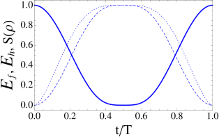
Figure 1: Entanglement of formation (solid curve) $E_{f}(\rho(t))$ for the system described by the quantum ensemble ${\cal A}(t)$ of Eq. (7). We also show the hidden entanglement $E_{h}({\cal A},t)$ (dashed curve), and the von Neumann entropy (dotted curve) $S(\rho(t))$.

As we can see from Fig. 1, the von Neumann entropy $S(\rho(t))$, which is equal to the quantum mutual information $I(\textsf{S}:\textsf{E})$ since we are considering an ensemble of pure states (see Sec. 2), exhibits a behavior very close to that of HE. This similarity has a simple explanation: We have an ensemble ${\cal A}(t)$ of maximally entangled states, so that the lack of knowledge about which state of the mixture we are dealing with is the only reason that prevents us from exploiting entanglement as a resource. Such lack of knowledge is correctly captured by the von Neumann entropy.

Let us now consider the same quantum operation described at the beginning of this section, but starting from a different initial state, in general mixed:

$$\rho_{0}=\eta|{\phi^{+}}\rangle\langle{\phi^{+}}|+(1-\eta)\Big{(}\frac{1}{2}|{00}\rangle\langle{00}|+\frac{1}{2}|{11}\rangle\langle{11}|\Big{)}.$$ (8)

That is, the system is prepared in the maximally entangled state $|{\phi_{+}}\rangle$ with probability $\eta$, or in one of the separable states $|{00}\rangle$ and $|{11}\rangle$, with equal probability $\frac{1}{2}(1-\eta)$, and the preparation record is disregarded or not available. In this case the quantum ensemble at time $t$ is

$${{\cal A}}(t)=\big{\{}\big{(}p_{i},\mathbb{U}_{i}(t)\rho_{0}\mathbb{U}^{\dagger}_{i}(t)\big{)}\big{\}}\,=\,\Big{\{}\Big{(}\frac{1}{2},\mathbb{U}_{x}(t)\rho_{0}\mathbb{U}_{x}^{\dagger}(t)\Big{)},\,\Big{(}\frac{1}{2},\mathbb{U}_{z}(t)\rho_{0}\mathbb{U}_{z}^{\dagger}(t)\Big{)}\Big{\}}.$$ (9)

The density operator which arises from such ensemble is $\rho(t)=\sum_{i}p_{i}\mathbb{U}_{i}(t)\rho_{0}\mathbb{U}^{\dagger}_{i}(t)$. The parameter $\eta$ allows us to set simultaneously the entanglement and the mixedness of the initial state $\rho_{0}$. When $\eta=1$ the system S is initially in a maximally entangled pure state and we recover the case discussed at the beginning of this section; when $\eta=0$, the initial state of S is a separable mixed state. We define the hidden entanglement associated with the ensemble (9) as

$$E_{h}({{\cal A}},t)=\sum_{i}p_{i}E(\mathbb{U}_{i}(t)\rho_{0}\mathbb{U}_{i}^{\dagger}(t))-E(\rho(t))=E_{f}(\rho_{0})-E_{f}(\rho(t)).$$ (10)

Such definition extends the hidden entanglement measure of Eq. (2) to ensemble of mixed states: The maximum entanglement which we can obtain at any time, once we retrieve the information about which operation the system undergoes, is just $E_{f}(\rho_{0})$ .

We plot in the top panels of Fig. 2 the entanglement of formation $E_{f}$ of the state $\rho(t)$ (left) and the hidden entanglement $E_{h}({{\cal A}},t)$ (right), for different values of the parameter $\eta$. For $\eta=1$ (solid curves) we recover the results of Fig. 1. For $\eta=0$ (dotted curves), there is no entanglement in the initial state and therefore no entanglement can be generated during the purely local time evolution, so both $E_{f}$ and $E_{h}$ are vanishing at any times. For $\eta=0.5$ (dashed curves), first the entanglement monotonically decreases until it sudden dies at $t/T\approx 0.33$ , then it revives after $t/T\approx 0.67$, up to its initial value. The entanglement decrease and its sudden death are consequences of our ignorance about the random operation $\mathbb{U}_{i}$ the system undergoes: if this information is provided not only the sudden death may be avoided, but also all the initial entanglement may be recovered at any time.

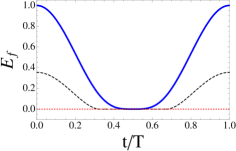
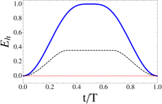
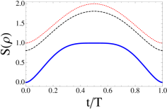
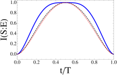
Figure 2: Entanglement of formation (top left panel), hidden entanglement (top right panel), von Neumann entropy (bottom left panel), and system-environment quantum mutual information (bottom right panel) for the ensemble (9), as a function of the time, for $\eta=1$ (solid curves), $0.5$ (dashed curves), and $0$ (dotted curve). Data for $\eta=1$ are the same as in Fig. 1 and are reported here for comparison.

In the bottom panels of Fig. 2 we show the von Neumann entropy $S$ of the state $\rho$ (left) and the system-environment quantum mutual information $I(\textsf{S}:\textsf{E})$ (right). For $\eta<1$, $S(\rho(t))$ exhibits a behavior which is qualitatively and quantitatively different from that of $E_{h}(\tilde{{\cal A}},t)$. For $\eta=0$, $S(\rho(t))$ varies in the range $[1,2]$, while the entanglement of formation and the hidden entanglement are vanishing at any times. For intermediate values, for instance $\eta=0.5$, $S(\rho(t))$ monotonically increases from the finite value $S(\rho_{0})$ up to its maximum value reached at $t=T/2$; in the same interval, $E_{h}$ starts from zero and saturates before $T/2$ to its maximum value $E_{f}(\rho_{0})$. This example shows that the system uncertainty, quantified by the von Neumann entropy, is not always connected to the possibility of recovering entanglement. By injecting classical information we reduce our lack of knowledge on the system, however such information does not always allow us to increase the system entanglement.

We now consider the quantum mutual information. As we have written in Sec. 2, it is possible to introduce a fictitious environment which simulates the action of our quantum operation. The system environment state is

$$\rho^{\textsf{SE}}(t)=\sum_{i}p_{i}|{x_{i}}\rangle\langle{x_{i}}|\otimes\mathbb{U}_{i}(t)\rho_{0}\mathbb{U}^{\dagger}_{i}(t).$$ (11)

The quantum mutual information between S and E is given by

$$I(\textsf{S}:\textsf{E}) =S(\rho(t))\,+\,S(\rho^{\textsf{E}}(t))\,-\,S(\rho^{\textsf{SE}}(t)))$$ (12)

$$=S(\rho(t))\,+\,H({p_{i}})\,-\,\Big{(}H({p_{i}})+\sum_{i}p_{i}S(\mathbb{U}_{i}(t)\rho_{0}\mathbb{U}^{\dagger}_{i}(t))\Big{)}=$$

$$=\,S(\rho(t))\,-\,S(\rho_{0}).$$

From Fig. 2, we can see that the quantum mutual information is scarcely sensitive to the entanglement that can be recovered. One can say that S and E develop the same degree of correlations as a function of the time, regardless of $\eta$, that is independently of the fact the system is initially prepared in an entangled state or in a separable state. In other words, from the value assumed by $I(S:E)$ one cannot in general estimate the amount of entanglement that is possible to recover at a given time by classical communication and local operations on the subsystems composing S.

4 Final remarks

The above considerations on the quantum mutual information tell us that non-Markovianity of system dynamics, which can be interpreted as a back-flow of information between S and E [25] and quantified [29, 30] in terms of negative time derivative of the coherent information, $\partial I(\textsf{S}:\textsf{E})/\partial t\,<\,0$, is only a necessary condition for entanglement revivals. Indeed we can have back-flow of classical information from the environment to the system without entanglement revivals, provided we are dealing with an ensemble of separable states for the system. We can conclude with the following statements about the occurrence of entanglement revivals when a system interacts with classical noise sources. In the case $E_{f}(t)=0$, the information we can acquire from the environment may be useful to recover some entanglement only if the quantum ensemble physically underlying the system dynamics has a non vanishing average entanglement. In a more general case, in the presence of a back-flow of information and $E_{f}(t)\neq 0$, we can identify a sufficient condition for entanglement revivals at time larger than $t$ by the requirement $E_{h}(t)>0$.

References

References

- [1] R. Lo Franco, B. Bellomo, E. Andersson and G. Compagno, Phys. Rev. A 85 (2012) 032318.
- [2] A. D’Arrigo, R. Lo Franco, G. Benenti, E. Paladino and G. Falci, arXiv:1207.3294 [quant-ph].
- [3] B. Bellomo, R. Lo Franco and G. Compagno, Phys. Rev. Lett. 99 (2007) 160502.
- [4] G. Falci, A. D’Arrigo, A. Mastellone and E. Paladino, Phys. Rev. Lett. 94 (2005) 167002.
- [5] G. Ithier, E. Collin, P. Joyez, P. J. Meeson, D. Vion, D. Esteve, F. Chiarello, A. Shnirman, Y. Makhlin, J. Schriefl and G. Schön, Phys. Rev. B 72 (2005) 134519.
- [6] J. Bylander, S. Gustavsson, F. Yan, F. Yoshihara, K. Harrabi, G. Fitch, D. G. Cory, Y. Nakamura, J-S. Tsai and W. D. Oliver, Nature Physics 7 (2011) 565.
- [7] F. Chiarello, E. Paladino, M. G. Castellano, C. Cosmelli, A. D’Arrigo, G. Torrioli and. G Falci, New J. Phys. 14 (2012) 023031.
- [8] R. Lo Franco, A. D’Arrigo, G. Falci, G. Compagno and E. Paladino, Phys. Scripta T147 (2012) 014019.
- [9] E. Paladino, Y. M. Galperin, G. Falci and B. L. Altshuler, preprint arXiv:1304.7925 [cond-mat.mes-hall], to be published in Rev. Mod. Phys..
- [10] J.-S. Xu, K. Sun, C.-F. Li, X.-Y. Xu, G.-C. Guo, E. Andersson, R. Lo Franco and G. Compagno, Nature Communications 4 (2013) 2851.
- [11] C. H. Bennett, D. P. DiVincenzo, J. A. Smolin and W. K. Wootters, Phys. Rev. A 54 (1996) 3824.
- [12] O. Cohen, Phys. Rev. Lett. 80 (1998) 2493.
- [13] H. Nha and H. J. Carmichael, Phys Rev. Lett. 93 (2004) 120408.
- [14] A. R. R. Carvalho, M. Busse, O. Brodier, C. Viviescas and A. Buchleitner, Phys. Rev. Lett. 98 (2007) 190501.
- [15] M. B. Plenio and S. Virmani, Quant. Inf. Comput. 7 (2007) 1.
- [16] R. Horodecki, P. Horodecki, M. Horodecki and K. Horodecki, Rev. Mod. Phys. 81 (2009) 865.
- [17] A. D’Arrigo, R. Lo Franco, G. Benenti, E. Paladino and G. Falci, Phys. Scr. T153 (2013) 014014.
- [18] J. Eisert, T. Felbinger, P. Papadopoulos, M. B. Plenio and M. Wilkens, Phys. Rev. Lett. 84 (2000) 1611.
- [19] G. Gour, Phys. Rev. A 75, (2007) 054301.
- [20] E. Mascarenhas, B. Marques, D. Cavalcanti, M. Terra Cunha and M. França Santos, Phys. Rev. A 81 (2010) 032310.
- [21] E. Mascarenhas, D. Cavalcanti, V. Vedral and M. França Santos, Phys. Rev. A 83 (2011) 022311.
- [22] S. Vogelsberger and D. Spehner, Phys. Rev. A 82 (2010) 052327.
- [23] A. Barchielli and M. Gregoratti, arXiv:1202.2041 [quant-ph], in Quantum probability and related topics, eds. L. Accardi and F. Fagnola (World Scientific, Singapore, 2012).
- [24] K. W. Murch, S. J. Weber, C. Macklin and I. Siddiqi, Nature 502 (2013) 211.
- [25] H-P. Breuer, E-M. Laine and J. Piilo, Phys. Rev. Lett. 103 (2009) 210401.
- [26] I. Devetak, IEEE Trans. Inf. Theory 51 (2005) 44.
- [27] M. A. Nielsen and I. L. Chuang, Quantum computation and quantum information (Cambridge University Press, Cambridge, 2000).
- [28] G. Benenti, G. Casati and G. Strini, Principles of quantum computation and information, vol. II (World Scientific, Singapore, 2007).
- [29] L. Mazzola, C. A. Rodriguez-Rosario, K. Modi and M. Paternostro, Phys. Rev. A 86 (2012) 010102(R).
- [30] S. Luo, S. Fu and H. Song, Phys. Rev. A 86 (2012) 044101.
- [31] M. Horodecki, P. Horodecki and R. Horodecki, Phys. Rev. Lett. 84 (2000) 2014.
- [32] W. K. Wootters, Phys. Rev. Lett. 80 (1998) 2245.
- [33] G. Vidal, W. Dür and J. I. Cirac, Phys. Rev. Lett. 89 (2002) 027901.