Conditioned limit laws for inverted max-stable processes

Abstract

Max-stable processes are widely used to model spatial extremes. These processes exhibit asymptotic dependence meaning that the large values of the process can occur simultaneously over space. Recently, inverted max-stable processes have been proposed as an important new class for spatial extremes which are in the domain of attraction of a spatially independent max-stable process but instead they cover the broad class of asymptotic independence. To study the extreme values of such processes we use the conditioned approach to multivariate extremes that characterises the limiting distribution of appropriately normalised random vectors given that at least one of their components is large. The current statistical methods for the conditioned approach are based on a canonical parametric family of location and scale norming functions. We study broad classes of inverted max-stable processes containing processes linked to the widely studied max-stable models of Brown-Resnick, Schlather and Smith, and identify conditions for the normalisations to either belong to the canonical family or not. Despite such differences at an asymptotic level, we show that at practical levels, the canonical model can approximate well the true conditional distributions.

Key-words: Asymptotic independence; Brown–Resnick process; conditional dependence; extremal Gaussian process; Hüsler–Reiss copula; inverted max-stable distribution; Smith process; spatial extremes
AMS subject classifications: Primary: 60GXX, Secondary: 60G70

1 Introduction

Extreme environmental events, such as hurricanes, heatwaves, flooding and droughts, can cause havoc to the people affected and typically result in large financial losses. The impact of this type of event is often exacerbated by the event being severe over a large spatial region. The statistical modelling of spatial extremes is a rapidly evolving area (davpadrib) and is crucial to understanding, visualizing and predicting the extremes of stochastic processes. The approach that is currently most used for modelling spatial extreme values assumes the environmental process is a max-stable process (haan84). The most widely used max-stable processes are the Smith (smit90b), Brown-Resnick (browresn77; kabletal09), the extremal Gaussian (schl02), and the extremal-$t$ (demarta2005; nikoetal09) processes.

Max-stable processes are the only non-trivial limit of point-wise normalised maxima of independent and identically distributed realisations of a stochastic processes. When max-stable processes are observed at a finite number of locations their joint distribution is a multivariate extreme value distribution, which is underpinned by the assumption of the original variables satisfying the dependence structure conditions of multivariate regular variation (resn87). Max-stable processes have marginal generalised extreme value distributions (cole01) and a complex non-negative dependence structure which has a restricted form. To understand this restriction, let $\{X_{M}(s),s\in\mathbb{R}^{2}\}$ be a spatial max-stable process with continuous marginal distribution functions $F_{s}$ and corresponding inverse denoted by $F_{s}^{\leftarrow}$. Then, if for any $s_{1},s_{2}\in\mbox{$\mathbb{R}$}^{2}$ where $X_{M}(s_{1})$ and $X_{M}(s_{2})$ are not independent, it follows that the dependence coefficient

$$\chi=\lim_{p\rightarrow 1}\Pr\left\{X_{M}(s_{2})>F_{s_{2}}^{\leftarrow}(p)\mid X_{M}(s_{1})>F_{s_{1}}^{\leftarrow}(p)\right\},$$

is positive. This property is termed asymptotic dependence; for max-stable processes it implies that the spatial properties of extreme events are independent of the severity of the event (davpadrib).

wadtawn12 introduced the class of inverted max-stable processes and these are used in davhusthi13. Any inverted max-stable process $\{X(s),s\in\mathbb{R}^{2}\}$ with unit exponential margins, i.e., for all $s\in\mathbb{R}^{2}$ and $x>0$, $\Pr(X(s)<x)=1-\exp(-x)$, $x>0$, can be represented by

$$X(s)=1/X_{F}(s)\quad s\in\mathbb{R}^{2},$$

where $\{X_{F}(s),s\in\mathbb{R}^{2}\}$ is a max-stable process with unit Fréchet margins, i.e., for all $s\in\mathbb{R}^{2}$ and $x>0$, $\Pr(X_{F}(s)<x)=\exp(-1/x)$. Thus, for all $s_{1},s_{2}\in\mathbb{R}^{2}$, the dependence structure between large $X(s_{1})$ and $X(s_{2})$ is equivalent to the dependence structure between small $X_{F}(s_{1})$ and $X_{F}(s_{2})$ and hence differs from the max-stable form. All non-perfectly dependent inverted max-stable processes are in the domain of attraction of spatially independent max-stable processes (see Section 2.1), meaning that their point-wise normalised maxima are independent, i.e., for all $s_{1},s_{2}\in\mathbb{R}^{2}$ , with $s_{1}\not=s_{2}$,

$$\lim_{n\rightarrow\infty}\Pr\left(\max_{i=1,\ldots,n}X_{i}(s_{1})-\log n<x_{1},\max_{i=1,\ldots,n}X_{i}(s_{2})-\log n<x_{2}\right)=\prod_{i=1}^{2}\exp\{-\exp(-x_{i})\},$$ (1)

for any $x_{1},x_{2}\in\mathbb{R}$, where $\{X_{i}(s),s\in\mathbb{R}^{2}\}$, $i=1,\ldots,n$ denotes a sequence of independent and identically distributed inverted max-stable processes with unit exponential margins.

To reveal the extremal dependence structure for asymptotically independent random variables, alternative asymptotic properties need to be studied. ledtawn96; ledtawn97 and resnick02 explore the joint tail through the limiting joint survivor function,

$$g(x_{1},x_{2})=\lim_{t\rightarrow\infty}\mathcal{L}(t)\exp\{t/\eta(s_{1},s_{2})\}\Pr\left\{X(s_{1})>x_{1}+t,X(s_{2})>x_{2}+t\right\}$$ (2)

where $0<\eta<1$, known as the coefficient of tail dependence, and $\mathcal{L}$ is a slowly varying function at $\infty$, are selected so that $0<g(x_{1},x_{2})<\infty$, and the dependence structure revealed by limit (2) is known as hidden regular variation. A weakness with this approach is that it fails to describe the behaviour of the $X(s_{2})$ values that occur with the largest values of $X(s_{1})$. Instead a conditioned approach is required which looks at a more subtle normalisation for $X(s_{2})$ that focuses on the region of the joint distribution which is most likely when conditioning on variable $X(s_{1})$ being large. This is the approach we take in this paper.

For a bivariate random variable $(X,Y)$ with unit exponential margins and general dependence structure the conditioned extremes limit theory of hefftawn04 and heffres07 is equivalent to the assumption that there exist location and scaling norming functions $a:\mathbb{R}_{+}\rightarrow\mathbb{R}$ and $b:\mathbb{R}_{+}\rightarrow\mathbb{R}_{+}$, such that, for any $x>0$ and $z\in\mbox{$\mathbb{R}$}$,

$$\lim_{u\rightarrow\infty}\Pr\left\{X-u>x,\{Y-a(X)\}/{b(X)}<z\mid X>u\right\}=\exp(-x)G(z),$$ (3)

where $G$ is a non-degenerate distribution function. To ensure $a$, $b$ and $G$ are uniquely defined the condition $\lim_{z\rightarrow\infty}G(z)=1$ is required, so $G$ places no mass at $+\infty$ but some mass is allowed at $-\infty$. For positively dependent random variables, hefftawn04 found that, for all the standard copula models studied by joe97 and Nelsen06, the norming functions $a(x)$ and $b(x)$, fell into the simple canonical parametric family

$$a(x)=\alpha x\quad\text{and}\quad b(x)=x^{\beta},$$ (4)

where $\alpha\in[0,1]$ and $\beta\in(-\infty,1)$. The case $\alpha=1$ and $\beta=0$ corresponds to $\chi>0$, whereas any other combination of $\alpha$ and $\beta$ gives $\chi=0$. With standard Laplace margins, keefpaptawn13 extended model class (4) to $-1\leq\alpha\leq 1$ to account for negatively dependent random variables when $\alpha\in[-1,0)$. However, this is not relevant for inverted max-stable processes as they are non-negatively dependent.

A key question is why have we made the restriction of unit exponential margins on the inverted max-stable process. In the style of copula methods (Nelsen06) we assume identical margins. Conditioned limit theory has studied limiting presentation (3) with the margins $(X,Y)$ taken as identically distributed Gumbel variables (hefftawn04), which is asymptotically equivalent to unit exponential margins but mathematically less clean, whereas eastoetawn12 take identically distributed generalised Pareto distributions. In contrast heffres07 work with $X$ in the domain of attraction of the generalised extreme value distribution distribution, but do not impose any constraint on $Y$, and find that it is not always possible to achieve an affine normalisation as in limit (3) after marginal transformation to identical margins. kulisoul14 consider $(X,Y)$ with margins that have regularly varying tails, with location function $a(x)=0$. Through the paper we also find that for broad and important classes of inverted max-stable processes, it is possible to achieve affine normalisations after transformation to identical exponential marginal variables. Furthermore, for some of these classes of inverted max-stable distributions limit (3) does not hold with margins that have regularly varying tails but holds with unit exponential margins. Thus our restriction to unit exponential margins provides all the necessary ground work for deriving conditioned limits with any marginal distributions for inverted max-stable processes. In Section 2.2 we discuss the implications of the marginal choice, and in particular show how once the limit relationship has been derived for unit exponential margins alternative limit results follow immediately for other marginal choices.

Canonical family (4) has been subject of criticism (Smit04) since the functions $a$ and $b$ seem to be ‘proof by example’ rather than a general result. heffres07 note that under assumption (3) and in unit exponential marginals,

$$\lim_{t\rightarrow\infty}b(t+x)/b(t)=\psi_{1}(x)\quad\text{and}\quad\lim_{t\rightarrow\infty}\left\{a(t+x)-a(t)\right\}/b(t)=\psi_{2}(x),$$

for any $x\in\mathbb{R}$, where $\psi_{1}$ and $\psi_{2}$ are real functions. For the canonical family (4), it readily follows that $(\psi_{1},\psi_{2})=(1,0)$ if $\beta>0$ and $(\psi_{1},\psi_{2})=(1,\alpha x)$ if $\beta=0$ and this condition is also satisfied by a range of regularly varying functions. However, no examples have been published to date other than the canonical form (4).

For simplicity we focus on bivariate characterisations of the inverted max-stable process, with all joint distributions following inverted bivariate extreme value distributions. For the rest of the paper we denote by $(X,Y)$ a bivariate random variable with inverted bivariate extreme value distribution with unit exponential margins and derive $a$, $b$ and $G$. We find classes of this family where the normalisation required to achieve property (3) either falls in the canonical family (4) or a more general form is required. Examples of the former include the inverted max-stable models with Schlather (schl02) and extremal-$t$ (demarta2005; nikoetal09) dependence models, and the latter include inverted max-stable model with Smith (smit90b) dependence model. We show that the distinction between these classes is determined by the behaviour of the spectral measure of the underlying max-stable process near its lower end point.

The statistical conditioned model of hefftawn04 assumes that the limiting relationship (3) holds exactly for all values $X>u$ for a suitably high threshold $u$ with the functions $a$ and $b$ in canonical form (4). This model has been found to fit well in various applications (pauletal06; keefST09; hila11; eastoetawn12; papatawn14). Our identification of the existence of the new classes that do not fall in canonical family (4) questions the validity of the generic use of the canonical family for statistical modelling. Therefore, we compare the new models with the current statistical approach of hefftawn04 and show, through simulation, that at practical levels, that the use of canonical family gives good approximations to the conditional distribution of the inverted max-stable model with Smith dependence and highlight examples where a good approximation does not hold.

The paper is structured as follows. In Section 2 we present the classes of max-stable and inverted max-stable distributions and explore the implications of deriving results on general margins. In Section 3 we present the conditional representation of the class of inverted max-stable distributions with spectral densities of the associated max-stable process being regularly varying and $\Gamma$-varying spectral densities at their lower end-point. In Section 4 we discuss the spatial extension of our results. Our derivations and proofs are included in the Appendix.

2 Bivariate inverted max-stable distributions

2.1 Max-stable and inverted max-stable distributions

Max-stable distributions arise naturally as the only non-degenerate limit distributions of appropriately normalised component-wise maxima of random vectors. In unit Fréchet margins, and for $x,y>0$, a bivariate max-stable distribution function is defined by

$$F(x,y)=\exp\left\{-V\left(x,y\right)\right\}=\exp\left[-\int_{0}^{1}\max\left\{w/x,(1-w)/y\right\}\,\mathrm{d}H(w)\right],$$ (5)

where $V$ is termed the exponent measure and $H$ is an arbitrary finite measure on $[0,1]$, known as the spectral measure, with total mass 2, satisfying the marginal moment constraint $\int_{0}^{1}w\,\mathrm{d}H(w)=1$. coletawn91 showed that if $F$ has a density, then $H(w)$ has spectral density $h(w)$ on the interior $(0,1)$ and can have mass $H(\{k\})$, $k=0,1$, on each of $\{0\}$ and $\{1\}$, given by rCl h(w) &= -∂2V∂x∂y(w,1-w)  0¡w¡1,

H({0}) = -y^2lim_x →0 ∂V∂y(x,y),  and  H({1}) = -x^2lim_y →0 ∂V∂x(x,y). As the class of bivariate max-stable distributions does not admit a finite dimensional parameterisation, a natural method for modelling the spectral measure $H$ of expression (5) relies on constructing parametric sub-classes of models that are flexible enough to approximate any member from the class (coletawn91; ballschla11). Two such sub-models are huslreis89 and schl02 max-stable distributions which have exponent measures, for $x,y>0$, rCl &V(x,y)=1xΦ{ λ2 + 1λlog(yx) } + 1yΦ{ λ2 + 1λ log(xy) }  λ∈(0,∞),

V(x,y)=12(1x + 1y) [1 + {1 - 2 (1+ρ)x y(x+y)2}^1/2]  ρ∈(-1,1) , respectively, where $\Phi$ is the cumulative distribution function of the standard normal distribution. These are the exponent measures of the pairwise distributions for the Smith and Schlather max-stable models respectively. The parameters $\lambda$ and $\rho$ control the strength of dependence. In particular, increasing and decreasing values of $\rho$ and $\lambda$, respectively, imply stronger dependence between $X$ and $Y$.

Given a max-stable distribution with exponent measure $V$ as in equation (5), the bivariate random variable $(X,Y)$ follows the inverted max-stable distribution with unit exponential margins if, for $x,y>0$, its joint survivor function is,

$$\Pr\left(X>x,Y>y\right)=\exp\left\{-V\left(1/x,1/y\right)\right\}.$$ (6)

As

$$\Pr\left(X>x,Y>x\right)=\exp(-x/\eta)=\{\Pr(X>x)\}^{1/\eta},\quad\eta=1/V(1,1)\in[1/2,1],$$

the inverted max-stable distributions are either perfectly dependent when $V(1,1)=1$ or asymptotically independent when $V(1,1)>1$. Specifically $\eta$ is the coefficient of tail dependence (ledtawn97). This property explains the independence in limit (1).

A range of results are available to study the conditional limit (3). In particular, heffres07, resnzebe14 and wadetal14 show that under various conditions, all of the followings limits are identical to $G(z)$ in limit (3):

$$\lim_{u\rightarrow\infty}\Pr\left\{\frac{Y-a(u)}{b(u)}<z\big{|}X>u\right\}=\lim_{u\rightarrow\infty}\Pr\left\{\frac{Y-a(X)}{b(X)}<z\big{|}X>u\right\}=\lim_{u\rightarrow\infty}\Pr\left\{\frac{Y-a(u)}{b(u)}<z\big{|}X=u\right\}.$$ (7)

These conditions hold for all inverted max-stable distributions if the associated spectral measure of the max-stable process places no point mass on the interval $(0,1)$, i.e., when $(X,Y)$ have a joint density. So we can use any of these limits to derive the forms of $a,b$ and $G$. Motivated by statistical considerations, we find that the use the last expression is most simple to use. However, this is the most restrictive in general as it requires the assumption of a joint density. As all the parametric max-stable models have joint densities so do the associated inverted max-stable distributions, so for us this is not restrictive. For using this third limit form it is helpful to note that the conditional survivor function is

$$\Pr\left(Y>y\mid X=x\right)=-V_{1}\left(1,x/y\right)\exp\left\{x-xV\left(1,x/y\right)\right\}\quad y>0,$$ (8)

where $V_{1}(x,y)=\partial V(x,y)/\partial x$.

2.2 Conditional representation with different marginal distributions

Let $(X,Y)$ be a bivariate random variable with common unit exponential margins and assume that limit (3) holds. Here we consider what this representation then implies for the extremal conditioned distribution of $Y_{H_{2}}\mid X_{H_{1}}$, where the bivariate random variable $(X_{H_{1}},Y_{H_{2}})$ has continuous marginal distribution functions $H_{1}$ and $H_{2}$ respectively and has identical copula to $(X,Y)$. For $i=1,2$, let $K_{i}(y)=-\log\{1-H_{i}(y)\}$ for $y\in\mathbb{R}$ and denote its inverse by $K_{i}^{\leftarrow}(y)=H_{i}^{\leftarrow}\{1-\exp(-y)\}$ for $y>0$. Then $(X_{H_{1}},Y_{H_{2}})=\{K_{1}^{\leftarrow}(X),K_{2}^{\leftarrow}(Y)\}$ have the required joint distribution and from limit (3) there exist functions $a:\mathbb{R}_{+}\rightarrow\mathbb{R}$ and $b:\mathbb{R}_{+}\rightarrow\mathbb{R}_{+}$ such that for all $z\in\mbox{$\mathbb{R}$}$

$$\lim_{u\rightarrow\infty}\Pr\left(Y_{H_{2}}<K_{2}^{\leftarrow}\left[a\{K_{1}(X_{H_{1}})\}+b\{K_{1}(X_{H_{1}})\}z\right]\mid X_{H_{1}}>u\right)=G(z)$$ (9)

for non-degenerate $G(z)$. Therefore, if we can find a location-scale normalisation when working with identical unit exponential margins then limit (9) shows that these results directly provide the appropriate conditioned limit for non-identically distributed marginals. Furthermore, limit (9) shows that in general margins a location-scale normalisation is not always possible even when it can be achieved with unit exponential margins. Of course the converse is true, but as we will see in Section 3 for the class of inverted max-stable distributions limit (3) holds with unit exponential margins, so limit (9) is useful to give the conditioned limits in other marginals.

To help understand the implications of limit (9) it is helpful to focus on specific forms for on $H_{1}$ and $H_{2}$. eastoetawn12 present limit (9) with identically distributed generalised Pareto distributions. kulisoul14 work with regularly varying tails. Focusing on the specific case of Pareto margins with $H_{i}(y)=1-y^{-\alpha_{i}}$ for $\alpha_{i}>0,\ y>1$ and $i=1,2$, limit (9) then becomes

$$\lim_{u\rightarrow\infty}\Pr\left\{Y_{H_{2}}<\exp\left(\left[a\{\alpha_{1}\log(X_{H_{1}})\}+b\{\alpha_{1}\log(X_{H_{1}})\}z\right]/{\alpha_{2}}\right)\,\Big{|}\,X_{H_{1}}>u\right\}=G(z)$$

so a location-scale normalisation in these margins can only be achieved with $b(y)\equiv 1$ and then only a scaling is required. Thus studying limit (3) with regularly varying tails only requires a scaling but critically cannot cover any cases where the $b$ scaling function when using unit exponential margins differs from $b(y)\equiv 1$. As we will see in Section 3, for the class of inverted max-stable distributions with unit exponential margins we have many classes where $b(y)\not=1$. Therefore, to reveal the full structure of the conditioned extremal behaviour of inverted max-stable distributions revealed by limit (3), it is essential to work in marginal variables which are tail equivalent to the unit exponential. Hence for the remainder of the paper we work exclusively with unit exponential margins acknowledging that these results apply directly with different margins using limit (9).

3 Conditional representations

3.1 Known representations

hefftawn04 explored the conditional representation (3) for the class of inverted max-stable distributions subject to the assumption that $H$ places all the mass in $(0,1]$ and that the spectral density is regularly varying rCl &h(w)∼L(w-w_ℓ) (w-w_ℓ)^t  as $w\rightarrow w_{\ell}\in[0,1/2)$, for $w_{\ell}=0$ and $\mathcal{L}(w)$ slowly varying at 0 with $\lim_{w\rightarrow w_{\ell}^{+}}\mathcal{L}(w-w_{\ell})=s>0$ and $t>-1$. Later, we consider more general formulations with $\mathcal{L}(w)\rightarrow\infty$ as $w\rightarrow 0^{+}$ and $w_{\ell}>0$. Under setting (1), the normalisation (4) required to give a non-degenerate limiting conditional law has $\alpha=0$, $\beta=(t+1)/(t+2)$ and the limit is of Weibull type, i.e.,

$$\lim_{u\rightarrow\infty}\Pr\left(Y<X^{\beta}z\mid X>u\right)=1-\exp\left\{-\frac{sz^{t+2}}{(t+1)(t+2)}\right\},\quad\text{for $z>0$.}$$ (10)

Examples of inverted max-stable models satisfying (10) include those with logistic and Dirichlet dependence structure coletawn91.

3.2 Regular variation at lower tail of spectral measure

We derive the conditional representation (3) for the class of inverted max-stable distributions covering more general spectral measures than those studied in Section 3.1. In particular, we explore model (1) and the effect on the normalising functions $a(x)$ and $b(x)$ when the spectral measure $H$ places its mass in a sub-region, $[w_{\ell},w_{u}]$ say, of $[0,1]$. Motivated by the Schlather distribution (5), for which the spectral measure places mass at $\{0\}$, we also explore the assumption of possible mass on the lower end point $w_{\ell}$ of $H$, but no point mass at any other $w\in(w_{\ell},w_{u})$. Although having mass at $w_{\ell}$, if $w_{\ell}>0$, implies that $(X,Y)$ do not have a joint density, as there is a singular component on the boundary of the sample space of $(X,Y)$, if this boundary is avoided then (8) is still valid. The results in the rest of the paper even hold if there is mass at some point in $(w_{\ell},w_{u})$, with modified proofs, but we avoid this unnecessary generalisation.

Lemma 1.

Let $w_{\ell}$, $w_{u}$, be the lower and upper end points, respectively, of the spectral measure $H$ of an inverted max-stable distribution (6), i.e.,

$$w_{\ell}=\inf\left\{{0\leq w<1/2}:H(w)\geq 0\right\},\quad w_{u}=\sup\left\{1/2<w\leq 1:H(w)\leq 2\right\},$$

and assume that, apart from the points $w_{\ell}$ and $w_{u}$, for which $H(w_{\ell}),H(w_{u})\geq 0$, the spectral measure is absolutely continuous with respect to the Lebesgue measure. Then, if $y/(x+y)\downarrow w_{\ell}$, for $y=y(x)$ a function of $x$, as $x\rightarrow\infty$, rCl V_1(1,x/y) &→ w_ℓ H({w_ℓ}) - 1.

In Lemma 1 the case of perfect positive dependence between $X$ and $Y$, i.e., $w_{\ell}=w_{u}=1/2$, is excluded since there can be no possible normalisation such that $G$ in expression (3) is non-degenerate. Proposition 1 gives the asymptotic form of the log-conditional survivor function of $Y\mid X=x$, for large $x$.

Proposition 1.

Under the conditions of Lemma 1 and for $h(w)$ as in expression (1), for $y/(x+y)\downarrow w_{\ell}\in[0,1/2)$ for $y=y(x)$ a function of $x$, as $x\rightarrow\infty$, we obtain that $\log\Pr\left(Y>y\mid X=x\right)$ is asymptotically equivalent to

$(i)$ for $H(\{w_{\ell}\})=0$, rCl & - x L(yx + y - w_ℓ) (yx + y - w_ℓ)^t+2/{(1-w_ℓ)(t+1)(t+2)},

$(ii)$ for $H(\{w_{\ell}\})>0$, rCl & log{1 - w_ℓ H({w_ℓ})} - (x+y)(yx+y - w_ℓ ) H({w_ℓ}).

As there is no contribution from the spectral density in expression (1), a general form for the normalisation can be obtained directly. General forms of the normalising functions $a(x)$ and $b(x)$ cannot be obtained from representation (1) without additional assumptions so it is helpful to consider a condition on the slowly varying function $\mathcal{L}$ at $0$. hefftawn04 results were based on the case of $\mathcal{L}$ having a finite right limit at $0$, Corollary 1 extends this.

Corollary 1.

Under the conditions of Proposition 1, limit (3) holds as follows

$(i)$ for $H(\{w_{\ell}\})=0$, then $a(x)=\{w_{\ell}/(1-w_{\ell})\}x$ and $b(x)=x^{(t+1)/(t+2)}\mathcal{L}\left\{x^{-1/(t+2)}\right\}^{-1/(t+2)}$ for $x>0$ and assuming that

$$\lim_{w\rightarrow 0^{+}}\frac{\mathcal{L}\left\{w\mathcal{L}(w)^{-\tau}\right\}}{\mathcal{L}(w)}=1,$$ (11)

for all $\tau\in(0,1)$, then

$$G(z)=1-\exp\left\{-\frac{(1-w_{\ell})^{3+2t}z^{t+2}}{(t+1)(t+2)}\right\}\quad\text{for $z>0$}.$$

$(ii)$ For $H(\{w_{\ell}\})>0$, then $a(x)=\{w_{\ell}/(1-w_{\ell})\}x$ and $b(x)=1$ for $x>0$, then

$$G(z)=1-\left\{1-w_{\ell}H(\{w_{\ell}\})\right\}\exp\left\{-(1-w_{\ell}){H(\{w_{\ell}\})}z\right\}\quad\text{for $z>0$},$$

and $G(z)=0$, for $z<0$, so $G(\{0\})=w_{\ell}H(\{w_{\ell}\})$.

Condition (11) is satisfied by a range of slowly varying functions, including those studied in Section 3.1 as well as by functions that approach $\infty$ when the argument tends to zero. Examples for $\mathcal{L}(w)$, with $\lim_{w\rightarrow 0^{+}}\mathcal{L}(w)=\infty$, satisfying condition (11) include $\log_{\kappa}\left(-\log w\right)$, $\kappa\in\mathbb{N}_{0}$, $\exp\left\{(-\log w)^{\nu}\right\}$, $\nu\in(0,1/2)$ and $\exp\left\{-\log w/\log\left(-\log w\right)\right\}$, where $\log_{k}$ is the iterated logarithm function defined recursively by $\log_{k}x=\log_{\kappa-1}\log x$, $\log_{0}x=x$ and $\log_{1}x=\log x$.

Remark 1.

For $\lim_{w\rightarrow 0^{+}}\mathcal{L}(w)=s>0$, all cases of norming functions $(i)$-$(ii)$ in Corollary 1 reduce, after absorbing $s$ into the limiting law, to the parametric class of Heffernan–Tawn, i.e., $a(x)+b(x)z=\alpha x+x^{\beta}z$, where $\alpha=w_{\ell}/(1-w_{\ell})\in[0,1)$ for $w_{\ell}\in[0,1/2)$ and $\beta=(t+1)/(t+2)\in[0,1)$ for $t\geq-1$. This is the first example to be known with both $\alpha$ and $\beta$ a function of parameters. 

Remark 2.

When $\lim_{w\rightarrow 0^{+}}\mathcal{L}(w)=\infty$ and subject to condition (11), the additional factor $\mathcal{L}\{x^{-1/(t+2)}\}^{-1/(t+2)}$ enters in the scaling function and reduces the rate of increase of $b(x)$ to $\infty$, as $x\rightarrow\infty$.

Another interesting case which is satisfied by many max-stable models that appear in the literature, is when $w_{\ell}=0$ and $H(\{w_{\ell}\})>0$ in case $(ii)$ of Corollary 1. In this case, $a(x)=0$ and $b(x)=1$ for all $x>0$ and the random variables $X$ and $Y$, conditionally on $X>u$, are near independent in the terminology of ledtawn97, with exact independence occurring when the limit distribution is unit exponential, i.e., when $H(\{w_{\ell}\})=1$. Two such max-stable models come from the extremal-$t$ (nikoetal09) and Gaussian-Gaussian (wadtawn12) processes, for which the exponent measures of their bivariate distributions are rCl V(x,y)& = 1xT_ν+1[(y/x)1/ν-ρ{(1-ρ2)/(ν+ 1)}1/2]+ 1yT_ν+1[(x/y)1/ν-ρ{(1-ρ2)/(ν+ 1)}1/2],

V(x,y)=12(1x+1y) + 12∫_$\mathbb{R}$^2{ϕ2(u)2x2 -2 ρ(h)ϕ2(u)ϕ2(h - u)x y + ϕ2(h - u)2y2}^1/2du, respectively, where $\nu>0$, $h\in\mbox{$\mathbb{R}$}^{2}_{+}$, $\rho(h)\in[-1,1]$ is a valid correlation function, $T_{\nu+1}$ is the distribution function of the standard-$t$ distribution with $\nu+1$ degrees of freedom, and $\phi_{2}$ is the density of the standard bivariate normal distribution with correlation $\rho(h)$. The corresponding mass on the lower end point $w_{\ell}=0$ of models (2) and (2) is

$$H(\{0\})=T_{\nu+1}\left[-\rho\left(\frac{\nu+1}{1-\rho^{2}}\right)^{1/2}\right]\quad\text{and}\quad H(\{0\})=\frac{1-\rho(h)}{2},$$

respectively. Table 1 gives a collection of other max-stable models, including the Schlather distribution (5), placing positive mass on $\{0\}$.

Table 1: The mass of the spectral measure on $\{0\}$ of bivariate exponent measures, from top to bottom, of mixed, asymmetric and asymmetric mixed logistic (tawn88), Schlather (schl02) and marsolki67a distributions. The final column shows the parameter space, $\Theta$, of the model.

$V(x,y)$	$H(\{0\})$	$\Theta$
$\left(\frac{1}{x}+\frac{1}{y}\right)-\frac{\theta}{x+y}$	$1-\theta$	$\theta\in(0,1)$
$\frac{1-\theta}{x}+\frac{1-\phi}{y}+\left\{\left(\theta/x\right)^{1/\alpha}+\left(\phi/y\right)^{1/\alpha}\right\}^{\alpha}$	$1-\phi$	$0\leq\theta,\phi,\alpha\leq 1$
$\frac{1}{x}+\frac{1}{y}-\frac{1}{xy}\left(\frac{1}{x}+\frac{1}{y}\right)^{-2}\left(\frac{\theta+\phi}{x}+\frac{2\phi+\theta}{y}\right)$	$1-\phi-\theta$	$\theta,\theta+3\phi>0$ and $\theta+\phi,\theta+2\phi\leq 1$
$\frac{1}{2}\left(\frac{1}{x}+\frac{1}{y}\right)\left[1+\left\{1-\frac{2\left(1+\rho\right)xy}{\left(x+y\right)^{2}}\right\}^{1/2}\right]$	$\left(1-\rho\right)/2$	$\rho\in(-1,1)$
$\alpha\left(\frac{1}{x}+\frac{1}{y}\right)+(1-\alpha)\max\left\{1/x,1/y\right\}$	$\alpha$	$0\leq\alpha\leq 1$

3.3 Inverted Smith model

In this section we focus on the limiting conditional representation of the inverted Smith model (5). This model has the same bivariate copula as the Húsler–Reiss distribution. The spectral measure of the Smith max-stable distribution places no mass on any $0\leq w\leq 1$, and the spectral density satisfies rCl &h(w) ∼exp(-λ2/8)λ  (2π)1/2 w^-3/2exp{-(logw)^2/(2λ^2)} as $w\rightarrow 0$. This corresponds to a different form than expression (1) or its more general forms of the slowly varying function $\mathcal{L}$. In particular, the spectral density is $\Gamma$-varying at 0 with auxiliary function

$$f(w)=-\lambda^{2}w/\log w.$$

As Proposition 2 shows, this example leads to a different form for the normalising functions $a(x)$ and $b(x)$ than the ones considered by hefftawn04.

Proposition 2.

Assume that $(X,Y)$ follows the inverted max-stable distribution (6) with exponent measure (5). Limit (3) holds with, for $x>0$ and $z\in\mathbb{R}$,

$$a(x)=x\exp\left\{-\lambda\,(2\log x)^{1/2}+\frac{\lambda\log\log x}{(2\log x)^{1/2}}+\frac{\lambda^{2}}{2}\right\},\,b(x)=a(x)/(\log x)^{1/2},$$ (12)

and

$$G(z)=1-\exp\left\{-\frac{\lambda}{(8\pi)^{1/2}}\exp\left(\sqrt{2}z/\lambda\right)\right\}.$$ (13)

Remark 3.

Limit distribution (13) is of reverted Gumbel type, which is different from the limits in Corollary 1. The rate of convergence to the limit is order $\log\log u/(\log u)^{1/2}$.

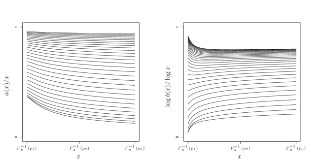
Figure 1: Plots of $a(x)/x$ and $\log b(x)/\log x$, $x>F_{X}^{-1}(0.87)$, where $a(x)$ and $b(x)$ are given by expression (12), for different values of $\lambda$ ranging from $0.01$ (bottom curves) to $20$ (top curves). The inverse of the unit exponential distribution function is $F_{X}^{\leftarrow}(p)=-\log(1-p)$, for $p\in(0,1)$. The values of $p_{1}$, $p_{2}$ and $p_{3}$ are 0.95, $1-10^{-7}$ and $1-10^{-13}$, respectively.

A natural question that arises from this counter-example relates to how well can the conditioned dependence model of hefftawn04 with canonical family (4) approximate the conditional distribution of $Y\mid X>u$, for large $u$, when the random vector $(X,Y)$ follows the inverted max-stable distribution with Smith dependence structure and unit exponential margins. To facilitate comparisons between the two models, Figure 1 shows the graphs of $a(x)/x$ and $\log b(x)/\log x$ where $a(x)$ and $b(x)$ are given by expression (12), for several values of the dependence parameter $\lambda$ and a range of $x$ values above the 0.87 unit exponential quantile. Both plots show that $a(x)/x$ and $\log b(x)/\log x$ are approximately constant for large $x$ so that the canonical class of norming functions is likely to approximate well $a(x)$ and $b(x)$ by $\alpha x$ and $x^{\beta}$, respectively. Subsequently, we simulated data from the inverted max-stable distribution with Smith dependence and fitted the conditioned dependence model using: $i)$ the canonical family (4) and $ii)$ the model implied by the norming functions (12), treating the functions (12) as a parametric model for the growth of $Y$ given large $X$. Our comparisons are based on the differences between the conditional quantile estimates of $Y\mid X=x$ from the two models.

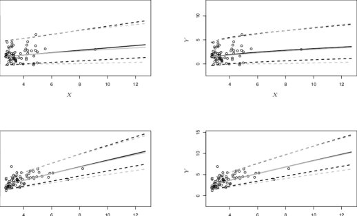
Figure 2: Conditional exceedances above the 0.935 unit exponential quantile from a simulated sample of size $10^{3}$ from the inverted max-stable distribution with Smith dependence and exponential margins for $\lambda=1.3$ (top) and $\lambda=0.3$ (bottom). The black lines correspond to averaged estimates from 100 simulations of the 0.025, 0.5 and 0.975 conditional quantiles of $Y\mid X=x$, $x>F_{X}^{-1}(0.935)$, using the Heffernan–Tawn model (4) (left) and the model constructed by the theoretical functions in expression (12) (right). Grey lines correspond to the theoretical 0.025, 0.5 and 0.975 conditional quantiles.

For both models, similar to hefftawn04, we used for the limiting law $G$ in expression (3) with the false working assumption of a normal distribution with mean and variance parameters. We considered two values for the dependence parameter, i.e., $\lambda=1.3$ (weak dependence) and $\lambda=0.3$ (strong dependence). For each $\lambda$, $10^{2}$ samples of size $10^{3}$ were generated from the inverted max-stable distribution with Smith dependence and the 0.025, 0.5 and 0.975 conditional quantile estimates of $Y\mid X=x$, for $x>F_{X}^{-1}(0.935)$, were computed from the two model fits, i.e., model (4) and the model defined by expression (12). The conditional quantile estimates are of the form $\hat{a}(x)+\hat{b}(x)\hat{z}_{p}$, where $\hat{a}(x)$, $\hat{b}(x)$ are maximum likelihood estimates and $\hat{z}_{p}$ is the $p$-th empirical quantile of $\hat{Z}=\{Y-\hat{a}(x)\}/\hat{b}(x)$, for large $x$. Figure 2 shows the averaged estimates of the conditional quantiles along with the theoretical conditional quantiles. Both models estimate the true conditional quantiles well and their behaviour is almost indistinguishable. This shows that the canonical model is flexible enough to approximate the conditional distribution of the inverted max-stable distribution with Smith dependence.

3.4 $\Gamma$-variation at lower tail of spectral density

Having identified a new form for the tail of the spectral density for the Smith max-stable model, we consider in this section the log-conditional survivor function of $Y\mid X=x$, under the assumption

$$h(w)\sim g(w-w_{\ell}),\quad\text{as $w\rightarrow w_{\ell}$},$$ (14)

where $g(w)\in\Gamma_{f}(0^{+})$. Similar to Section 3.2, we consider the assumption of possible mass at the lower end point $w_{\ell}$. Our findings are based on the assumptions of a differentiable spectral density $h$ and Lemma 2.

Lemma 2.

Let $g:\mbox{$\mathbb{R}$}^{+}\rightarrow\mbox{$\mathbb{R}$}^{+}\in\Gamma_{f}(0^{+})$ and $U(w)\in R_{\nu}(0^{+})$, $\nu\in\mbox{$\mathbb{R}$}$. Assume further that there exists an $\epsilon>0$ such that $U$ and $g$ are $C^{\infty}(0,\epsilon)$ functions with

$$\lim_{w\rightarrow 0^{+}}\frac{g^{\prime}(w)}{g(w)^{2}}\int_{0}^{w}g(s)~{}\mathrm{d}s$$ (15)

existing. Then
$(i)$   $U(w)g(w)\in\Gamma_{f}(0^{+})$.
$(ii)$  Define $f(w)=g(w)/g^{\prime}(w)$, $w>0$. Then, $f$ is an auxiliary function for $g$.
$(iii)$ For $f(w)$ as in $(ii)$, rCl (∫_0^w U(s) g(s) ds)/{U(w)f(w)g(w)} &= 1 - (U f)’(w)U(w) + {(Uf)’f}’(w)U(w) - ⋯

= 1 + o(1),  as $w\rightarrow 0^{+}$ .

Proposition 3 gives the asymptotic form of the log-conditional survivor function.

Proposition 3.

Under the conditions of Lemma 1 and for $h(w)$ as in expression (14), for $y/(x+y)\downarrow w_{\ell}\in[0,1/2)$ for $y=y(x)$ function of $x$, as $x\rightarrow\infty$, we obtain that $\log\Pr\left(Y>y\mid X=x\right)$ is asymptotically equivalent to

$(i)$ for $H(\{w_{\ell}\})=0$, rCl & - (x+y) f^2(yx+y-w_ℓ) h(yx+y),

$(ii)$ for $H(\{w_{\ell}\})>0$, rCl & log{1 - w_ℓ H({w_ℓ})} - (x+y)(yx+y - w_ℓ ) H({w_ℓ}).

As an example, we explore a new class of spectral densities that are more flexible than the spectral density (3.3) of the inverted max-stable distribution with Smith dependence. Specifically, consider for $\gamma>0$, $\delta\in\mathbb{R}$ and $\kappa>0$, the $\Gamma_{f}(0^{+})$-varying function rCl &h(w)∼w^δexp(-κw^-γ)  as $w\rightarrow 0^{+}$, with auxiliary function

$$f(w)=\left(\kappa\gamma\right)^{-1}w^{1+\gamma}.$$ (16)

Proposition 4 gives the normalising functions and limiting conditional distribution for this example.

Proposition 4.

Assume that $(X,Y)$ follows the inverted max-stable distribution (6) with spectral measure $H$ with $w_{\ell}=0$ and $H(\{0\})=0$, and spectral density $h$ that satisfies expression (3). Limit (3) holds with, for $x>0$ and $z\in\mathbb{R}$

$$a(x)=x\kappa^{1/\gamma}\left(\log x\right)^{-1/\gamma}\left[1+\gamma^{-2}\left\{\delta+2(1+\gamma)\right\}\frac{\log\log x}{\log x}\right],\,b(x)=x\left(\log x\right)^{-1-1/\gamma},$$ (17)

and

$$G(z)=1-\exp\left[-\left\{\kappa^{(\delta+2)/\gamma}/\gamma^{2}\right\}\exp\left(\gamma\kappa^{-1/\gamma}z\right)\right].$$ (18)

Remark 4.

Similarly with the inverted max-stable with Smith dependence, the limiting conditional distribution (18) is of reverted Gumbel type and the norming functions (17) do not belong to the Heffernan-Tawn parametric family. The rate of convergence to the limit is order $\log\log u/\log u$.

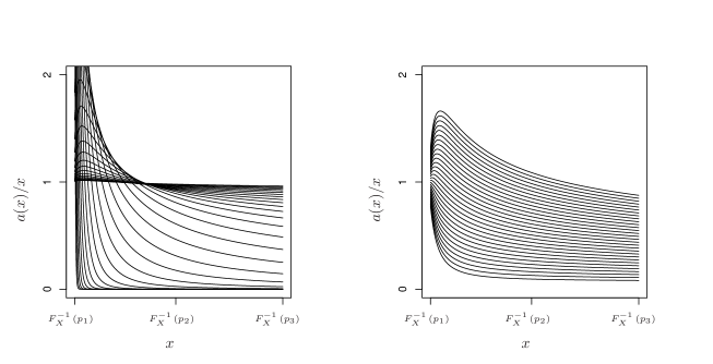
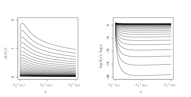
Figure 3: Plots of $a(x)/x$ for different values of the parameters $\gamma$ (top left), $\kappa$ (top right) and $\delta$ (bottom left) and $\log b(x)/\log x$ (bottom right), $x>F_{X}^{-1}(0.87)$. The inverse of the unit exponential distribution function is $F_{X}^{\leftarrow}(p)=-\log(1-p)$, for $p\in(0,1)$. The values of $p_{1}$, $p_{2}$ and $p_{3}$ are 0.95, $1-10^{-7}$ and $1-10^{-13}$, respectively.

Figure 3 shows the graphs of functions $a(x)/x$ and $\log b(x)/\log x$, for several values of the parameters $\gamma$, $\delta$, $\kappa$, and large $x$. Large values of $\gamma$ correspond to strong dependence between $X$ and $Y$ so that $a(x)/x$ is nearly constant and equal to $1$ for large $x$. Small values of $\gamma$ correspond to independence with sharp decrease of $a(x)/x$ to $0$ as $x$ increases. Intermediate values of $\gamma$ correspond to mild-moderate dependence of $X$ and $Y$ with $a(x)/x$ having a turning point and decaying as $x$ increases. Parameters $\kappa$ and $\delta$, seem to have similar effect with larger values corresponding to increasing dependence. Last, $\log b(x)/\log x$ is approximately constant with large $x$. Comparing with the canonical family (4), the degree of approximation of $a(x)$ and $b(x)$ by $\alpha x$ and $x^{\beta}$ is not especially good for $a(x)$. To our knowledge, there is no current parametric model for the max-stable process with spectral density satisfying expression (3).

4 Spatial extensions

engeetal2014 have found considerable insights can be gained by studying max-stable processes conditioned on the process being extreme at a fixed point, $s^{*}\in\mathbb{R}^{2}$ say. For $\{X(s);s\in\mathbb{R}^{2}\}$ an inverted max-stable processes with unit exponential margins a similar approach requires the existence of location and scaling norming functions $a_{s}:\mathbb{R}_{+}\rightarrow\mathbb{R}$ and $b_{s}:\mathbb{R}_{+}\rightarrow\mathbb{R}_{+}$, for all $s\in\mathbb{R}^{2}$, such that, for any $x>0$ and $\{z_{s}\in\mbox{$\mathbb{R}$},s\in\mathbb{R}^{2}\}$,

$$\lim_{u\rightarrow\infty}\Pr\left[X(s^{*})-u>x,\frac{X(s)-a_{s}\{X(s^{*})\}}{{b_{s}\{X(s^{*})\}}}<z_{s},s\in\mathbb{R}^{2}\backslash\{s^{*}\}\mid X(s^{*})>u\right]=\exp(-x)G(\boldsymbol{z}),$$ (19)

where $G$ is an infinite-dimensional joint distribution function that is non-degenerate in all univariate margins and $\boldsymbol{z}=\{z_{s},s\in\mathbb{R}^{2}\backslash\{s^{*}\}\}$.

From our working in this paper we have derived the forms of $(a_{s},b_{s})$ and $G_{s}$, the marginal of $G$, as these features are determined uniquely by the bivariate joint distributions of the inverted max-stable process. Thus all that remains to fully characterize limit (19) is to derive the infinite-dimensional dependence structure of $G$.

Here a complication arises as for most max-stable process models only the bivariate marginal distributions are available in closed form (davpadrib). Maybe future work can explore approaches that engeetal2014 have used to get around this issue for max-stable process. However, for the moment we restrict ourselves to consider the one well-known max-stable process which has closed form trivariate marginal distributions, the Smith process (see gentetal11). In this case we find that the associated bivariate limit $G_{s_{1},s_{2}}(z_{1},z_{2})=G_{s_{1}}(z_{1})G_{s_{2}}(z_{2})$, thus $G$ factorises; corresponding to asymptotic conditional independence in the terminology of hefftawn04. It follows that the infinite-dimensional $G$ will also factorise. Thus in this case all the dependence structure of the inverted max-stable processes is absorbed in the location-scale functions. Identifying which classes of max-stable process possess this asymptotic conditional independence for $G$ is an interesting line of future research.

5 Appendix

5.1 Proof of Lemma 1

For $s/(s+t)\in(w_{\ell},w_{u})$, the partial derivative of the exponent measure is equal to rCl ∂V (s,t)∂s& = ∂∂s [ ∫_ss+t^w_u (w/s)dH(w) + ∫_w_ℓ^ss+t {(1-w)/t}dH(w)]

= ∂∂s [ ∫_[ss+t,w_u) (w/s)h(w)dw + ∫_(w_ℓ,ss+t] {(1-w)/t} h(w)dw ] - (w_u/s^2) H({w_u})

= -∫_[ss+t,w_u) (w/s^2)h(w)dw - (w_u/s^2) H({w_u}), which, under the assumption of $y/(x+y)\downarrow w_{\ell}$, as $x\rightarrow\infty$, yields

$$V_{1}(1,x/y)\rightarrow-\int_{w_{\ell}}^{w_{u}}wh(w)\mathrm{d}w-w_{u}H(\{w_{u}\}),$$ (20)

as $x\rightarrow\infty$. Using the moment constraint (5) we have that

$$\int_{w_{\ell}}^{w_{u}}wh(w)\mathrm{d}w=\int_{\left(w_{\ell},w_{u}\right)}wh(w)\mathrm{d}w=1-w_{\ell}H(\{w_{\ell}\})-w_{u}H(\{w_{u}\}),$$

which yields equation (1), after combining with equation (20).

5.2 Proof of Proposition 1

Working similarly to the proof of Lemma 1, we get, after combining equations (8) and (1), that for $c(x,y)=y/\{x+y\}$, $d(x,y)=\{x+y\}/\{(1-w_{\ell})y-w_{\ell}x\}$, the log-conditional survivor, $\log\left\{\Pr\left(Y>y\mid X=x\right)\right\}$, is equal to
$(i)$ for $H(\{w_{\ell}\})=0$, rCl & (x+y)∫_w_ℓ^c(x,y) w L(w-w_ℓ) (w-w_ℓ)^t dw - y∫_w_ℓ^c(x,y) L(w-w_ℓ)(w-w_ℓ)^t  dw

= (x+y)∫_d(x,y)^∞ L(1/s) s^-(t+3) ds + {w_ℓ x - (1-w_ℓ) y}∫_d(x,y)^∞ L(1/s)s^-(t+2)  ds. For $t>-1$, $d(x,y)\rightarrow\infty$, $c(x,y)\rightarrow w_{\ell}$, as $x\rightarrow\infty$, we have, from Karamata’s theorem (resn87, pg. 17), that the last expression is asymptotically equivalent to rCl & (x+y)(t+2) {d(x,y)}^-(t+2) L{1/d(x,y)} + {wℓx - (1-wℓ)y}(t+1) {d(x,y)}^-(t+1) L{1/d(x,y)}, as $x\rightarrow\infty$, which simplifies to expresion (1).
$(ii)$ for $H(\{w_{\ell}\})>0$,

$$\log\left\{1-w_{\ell}H(\{w_{\ell}\})\right\}+\left\{w_{\ell}x-(1-w_{\ell})y\right\}H(\{w_{\ell}\})$$

.

5.3 Proof of Proposition 2

Let $\phi$ be the probability density function of the standard normal distribution. Assuming $y\rightarrow\infty$ as $x\rightarrow\infty$ with $y/x\rightarrow 0$, we have from expression (8), Lemma 1 and Mill’s ratio, that for large $x$, the log-conditional survivor, $\log\Pr\left(Y>y\mid X=x\right)$, is approximately equal to rCl & x - x[1 - ϕ{λ2+ 1λlog(x/y)}λ2+ 1λlog(x/y)] + y ϕ{λ2- 1λlog(x/y)}λ2- 1λlog(x/y)

= x ϕ{λ2+ 1λlog(x/y)}λ2+ 1λlog(x/y) [1 + yxϕ{λ2- 1λlog(x/y)}ϕ{λ2+ 1λlog(x/y)} {λ2+ 1λlog(x/y)}{λ2- 1λlog(x/y)}]

= x ϕ{λ2+ 1λlog(x/y)}λ2+ 1λlog(x/y) [1 + {λ2+ 1λlog(x/y)}{λ2- 1λlog(x/y)}]

≐ -c (x y)^1/2ϕ{1λlog(y/x)}{1λlog(y/x)}2[1 + O{(logx)^-1}], where $c=\lambda\exp\left(-\lambda^{2}/8\right)$. Now, let $z\in\mbox{$\mathbb{R}$}$ and $y=a(x)+b(x)z$, where $a(x)$ and $b(x)$ are given by equations (12). We have, as $x\rightarrow\infty$, rCl (xy)