Information Theory and Image Understanding: An Application to Polarimetric SAR Imagery

Abstract

This work presents a comprehensive examination of the use of information theory for understanding Polarimetric Synthetic Aperture Radar (PolSAR) images by means of contrast measures that can be used as test statistics. Due to the phenomenon called ‘speckle’, common to all images obtained with coherent illumination such as PolSAR imagery, accurate modelling is required in their processing and analysis. The scaled multilook complex Wishart distribution has proven to be a successful approach for modelling radar backscatter from forest and pasture areas. Classification, segmentation, and image analysis techniques which depend on this model have been devised, and many of them employ some kind of dissimilarity measure. Specifically, we introduce statistical tests for analyzing contrast in such images. These tests are based on the chi-square, Kullback-Leibler, Rényi, Bhattacharyya, and Hellinger distances. Results obtained by Monte Carlo experiments reveal the Kullback-Leibler distance as the best one with respect to the empirical test sizes under several situations which include pure and contaminated data. The proposed methodology was applied to actual data, obtained by an E-SAR sensor over surroundings of Weßling, Bavaria, Germany.

I Introduction

The aim of remote sensing is to capture and to analyze scenes of the Earth. Among the remote sensing technologies, Polarimetric Synthetic Aperture Radar (PolSAR) has achieved a prominent position (Lee and Pottier, 2009).

In general, PolSAR data are the result of the following procedure: orthogonally polarized electromagnetic pulses are transmitted towards a target, and the returned echo is recorded with respect to each polarization (Lopez-Martinez and Fabregas, 2003). Such data are processed in order to generate images and, as a consequence of the coherent illumination, they are contaminated with fluctuations on its detected intensity called ‘speckle’. Although speckle is a deterministic phenomenon since it is fully reproducible, it has the effect of a random noise. These alterations can significantly degrade the perceived image quality, as much as the ability of extracting information from the data.

Defining a stochastic identity for modeling PolSAR image regions is an important pre-processing step (Conradsen et al., 2003). The scaled multilook complex Wishart distribution has been successfully employed as a statistical model for homogeneous regions in PolSAR imagery (Frery et al., 2011). Several statistical image processing techniques use this distribution for segmentation (Beaulieu and Touzi, 2004), classification (Kersten et al., 2005), and boundary detection (Schou et al., 2003), to name a few applications.

Any parametric approach requires parameter estimation. The scaled multilook complex Wishart law is indexed by a scalar known as the number of looks and a Hermitian complex matrix. These quantities can be estimated by a number of techniques, but a single scalar measure would be more useful when dealing with samples from images. Such measure can be referred to as ‘contrast’ if it provides means for discriminating different types of targets (Gambini et al., 2006, 2008; Goudail and Réfrégier, 2004). Suitable measures of contrast not only provide useful information about the image scene but also assume a pivotal role in several image analysis procedures (Schou et al., 2003).

Recent years have seen an increasing interest in adapting information-theoretic tools to image processing (Goudail and Réfrégier, 2004). In particular, the concept of stochastic divergence (Liese and Vajda, 2006) has found applications in areas as diverse as image classification (Puig and Garcia, 2003), cluster analysis (Mak and Barnard, 1996), and multinomial goodness-of-fit tests (Zografos et al., 1990). Coherent polarimetric image processing has also benefited, since divergence measures can furnish methods for assessing segmentation algorithms (Schou et al., 2003). Morio et al. (2009) analyzed the Shannon entropy for the characterization of polarimetric imagery considering the circular multidimensional Gaussian distribution. In a previous work (Nascimento et al., 2010), several parametric methods based on the class $(h,\phi)$-divergences were proposed and submitted to a comprehensive examination.

The aim of this work is to assess the contrast capability of hypothesis tests based on stochastic distances between statistical models for PolSAR images. Analytic expressions for the $\chi^{2}$, Kullback-Leibler, Rényi (of order $\beta$), Bhattacharyya, and Hellinger distances between scaled multilook complex Wishart distributions in their most general way are derived. Subsequently, such measures are penalized by coefficients which depend on the size of two distinct samples, leading to the proposal of new homogeneity tests.

The performance of these five new hypothesis tests is analyzed by means of their observed test sizes using Monte Carlo in several possible scenarios including pure and contaminated data. This methodology is assessed with real data obtained by the E-SAR sensor.

The remainder of this paper is organized as follows. In Section II, we introduce the image statistical modeling for the polarimetric covariance matrix. The hypothesis testing method proposed by Salicrú et al. (1994) is adapted for dealing with Hermitian positive definite matrix models in Section III. Section IV presents computational results obtained from synthetic and actual data analysis. The main conclusions are then summarized in Section V.

II A model for polarimetric data: the scaled multilook complex Wishart distribution

The PolSAR processing results in a complex scattering matrix, which is defined by intensity and relative phase data. In strict terms such matrix has possibly four distinct complex elements, namely $S_{\text{VV}}$, $S_{\text{VH}}$, $S_{\text{HV}}$, and $S_{\text{HH}}$. However, under the conditions of the reciprocity theorem (Ulaby and Elachi, 1990), the scattering matrix can be simplified to a three-component vector, since $S_{\text{HV}}=S_{\text{VH}}$. Thus, we have a scattering vector

$$\bm{s}=[S_{\text{VV}}\quad S_{\text{VH}}\quad S_{\text{HH}}]^{t},$$

where $(\cdot)^{t}$ indicates vector transposition. Freeman and Durden (1998) presented an important description of this three-component representation. As discussed by Goodman (1963), the multivariate complex Gaussian distribution can adequately model the statistical behaviour of $\bm{s}$. This is called ‘single-look PolSAR data representation’ and hereafter we assume that the scattering vector has the dimension $p$, i.e., $\bm{s}=[S_{1}\quad S_{2}\quad\ldots\quad S_{p}]^{t}$.

Polarimetric data is usually subjected to multilook processing in order to improve the signal-to-noise ratio. To that end, Hermitian positive definite matrices are obtained by computing the mean over $N$ independent looks of the same scene. This results in the sample covariance matrix $\bm{Z}$ given by (Anfinsen et al., 2009)

$$\bm{Z}=\frac{1}{L}\displaystyle\sum_{i=1}^{L}\bm{s}_{i}\bm{s}_{i}^{\text{H}},$$

where $L$ is the number of looks, $\bm{s}_{i}$, $i=1,2,\ldots,L$, and $(\cdot)^{\text{H}}$ represents the complex conjugate transposition. The sample covariance matrix follows a scaled multilook complex Wishart distribution with parameters $\bm{\Sigma}$ and $L$ as parameters, characterized by the following probability density function:

$$f_{\bm{Z}}(\bm{Z}^{\prime};\bm{\Sigma},L)=\frac{L^{pL}|\bm{Z}^{\prime}|^{L-p}}{|\bm{\Sigma}|^{L}\Gamma_{p}(L)}\exp\{-L\operatorname{tr}(\bm{\Sigma}^{-1}\bm{Z}^{\prime})\},$$ (1)

where $\Gamma_{p}(L)=\pi^{p(p-1)/2}\prod_{i=0}^{p-1}\Gamma(L-i)$, $\Gamma(\cdot)$ is the gamma function, $\operatorname{tr}(\cdot)$ represents the trace operator, $|\cdot|$ denotes the determinant operator, $\bm{Z}^{\prime}$ denotes a single-outcome of $\bm{Z}$, the covariance matrix of $\bm{Z}$ is given by

$$\bm{\Sigma}=\operatorname{E}\{\bm{s}\bm{s}^{*}\}={\left[\begin{array}[]{cccc}\operatorname{E}\{S_{1}S_{1}^{*}\}&\operatorname{E}\{S_{1}S_{2}^{*}\}&\cdots&\operatorname{E}\{S_{1}S_{p}^{*}\}\\ \operatorname{E}\{S_{2}S_{1}^{*}\}&\operatorname{E}\{S_{2}S_{2}^{*}\}&\cdots&\operatorname{E}\{S_{2}S_{p}^{*}\}\\ \vdots&\vdots&\ddots&\vdots\\ \operatorname{E}\{S_{p}S_{1}^{*}\}&\operatorname{E}\{S_{p}S_{2}^{*}\}&\cdots&\operatorname{E}\{S_{p}S_{p}^{*}\}\end{array}\right]},$$

where $\operatorname{E}\{\cdot\}$ and $(\cdot)^{*}$ denote expectation and complex conjugation, respectively. This distribution is denoted by $\bm{Z}\sim\mathcal{W}(L,\bm{\Sigma})$ and it satisfies $\operatorname{E}(\bm{Z})=\bm{\Sigma}$ (Anfinsen et al., 2009).

Lee et al. (1994) derived many marginal distributions of the $\mathcal{W}(L,\bm{\Sigma})$ law and their transformations.

II-A Interpretability of the parameters $\bm{\Sigma}$ and $L$ in PolSAR images

Parameters $\bm{\Sigma}$ and $L$ possess physical meaning.

The diagonal elements of $\bm{\Sigma}$ convey the brightness information of the respective channels. On its turn, an increasing number of looks $L$ implies better image signal-to-noise ratios. Figure 1 illustrates the influence of these parameters on simulated PolSAR images of size $100\times 100$ pixels. Such synthetic images are generated from scaled multilook complex Wishart law with following parameters: $L\in\{3,12\}$ and $k\in\{0,5,10,15\}$ such that $\bm{\Sigma}=(1+k)B$, where

$$B={\left[\begin{array}[]{ccc}360932&11050+3759\textbf{i}&63896+1581\textbf{i}\\ &98960&6593+6868\textbf{i}\\ &&208843\end{array}\right]},$$ (2)

where i is the imaginary unit. Only the upper triangle and the diagonal are displayed because this covariance matrix $\bm{\Sigma}$ is Hermitian and, therefore, the remaining elements are the complex conjugates. This matrix was observed in (Frery et al., 2010) for representing PolSAR data of forested areas. As shown in Figure 1, images with $L=12$ are less affected by speckle, and the brighter are the ones indexed by $k=15$, i.e., with lager determinants. In this image, the HH (HV, VV, respectively) intensity was associated to the red (green, blue respectively) channel in order to compose a false color display.

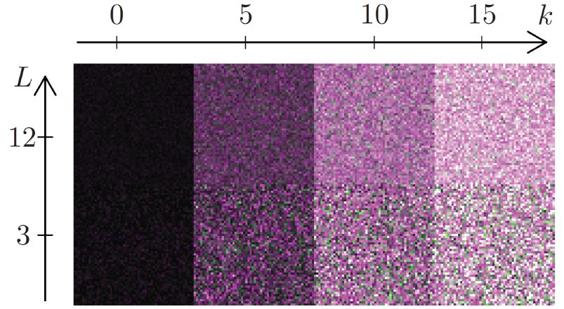
Figure 1: Simulated PolSAR images following scaled multilook complex Wishart law with parameters $L=\{3,12\}$ and $k=\{0,5,10,15\}$ such that $\bm{\Sigma}=(1+k)B$.

II-B Maximum likelihood estimation under the Wishart model

Let $\bm{Z}_{k}$ be a random matrix which follows a scaled multilook complex Wishart law with parameters $\bm{\gamma}=[L,\operatorname{vec}(\bm{\Sigma})^{t}]^{t}$, where $\operatorname{vec}(\cdot)$ is the column stacking vectorisation operator. Its log-likelihood function is expressed by

$$\ell_{k}(\bm{\gamma})=pL\log L+(L-p)\log|\bm{Z}_{k}|-L\log|\bm{\Sigma}|-\frac{p(p-1)}{2}\log\pi-\sum_{k=0}^{p-1}\log\Gamma(L-k)-L\operatorname{tr}(\bm{\Sigma}^{-1}\bm{Z}_{k}).$$

According to Hjorungnes and Gesbert (2007), $\partial\ell_{k}(\bm{\gamma})/\partial\operatorname{vec}(\bm{\Sigma})=\operatorname{vec}(\partial\ell_{k}(\bm{\gamma})/\partial\bm{\Sigma})$ then, the score function based on $\bm{Z}_{k}$ is given by

$$\nabla\ell_{k}(\bm{\gamma})=\left\{\begin{array}[]{l}p(\log L+1)+\log|\bm{Z}_{k}|-\log|\bm{\Sigma}|-\sum_{i=0}^{p-1}\psi^{(0)}(L-i)-\operatorname{tr}\big{(}\bm{\Sigma}^{-1}\bm{Z}_{k}\big{)},\\ \\ L\operatorname{vec}\big{(}\bm{\Sigma}^{-1}\bm{Z}_{k}\bm{\Sigma}^{-1}-\bm{\Sigma}^{-1}\big{)}.\end{array}\right.$$

In the sequel we present the derivation of (a1) the Hessian matrix $\mathcal{J}(\bm{\gamma})$, (a2) the Fisher information matrix $\mathcal{K}(\bm{\gamma})$, and (a3) the Cramér-Rao lower bound $\mathcal{C}(\bm{\gamma})$. To that end, the following quantity plays a central role:

$$\mathcal{J}_{\bm{\Sigma}\bm{\Sigma}}=\frac{\partial}{\partial\operatorname{vec}(\bm{\Sigma})^{*}}\Big{\{}\operatorname{vec}\Big{(}\frac{\partial\ell_{k}(\bm{\gamma})}{\partial\bm{\Sigma}}\Big{)}^{t}\Big{\}}.$$

Anfinsen et al. (2009) showed that

$$T_{1}=-\frac{\partial\{\bm{\Sigma}^{-1}\bm{Z}\bm{\Sigma}^{-1}\}}{\partial\bm{\Sigma}}=-\bm{\Sigma}^{-1}\otimes\bm{\Sigma}^{-1}\bm{Z}\bm{\Sigma}^{-1}-\bm{\Sigma}^{-1}\otimes\bm{\Sigma}^{-1}\bm{\Sigma}^{-1}\bm{Z},$$

where $\otimes$ denotes the Kronecker product. Moreover, it is known that (Hjorungnes and Gesbert, 2007) $T_{2}=\partial\bm{\Sigma}^{-1}/\partial\bm{\Sigma}=-\bm{\Sigma}^{-1}\otimes\bm{\Sigma}^{-1}$. Thus, we have that

$$\mathcal{J}_{\Sigma\Sigma}=L\{T_{2}-T_{1}\}=L\{\bm{\Sigma}^{-1}\otimes\bm{\Sigma}^{-1}-\bm{\Sigma}^{-1}\otimes\bm{\Sigma}^{-1}\bm{Z}\bm{\Sigma}^{-1}-\bm{\Sigma}^{-1}\otimes\bm{\Sigma}^{-1}\bm{\Sigma}^{-1}\bm{Z}\}.$$ (3)

From equation (3), it is possible to obtain that $\mathcal{K}_{\Sigma\Sigma}=\operatorname{E}\{-\mathcal{J}_{\Sigma\Sigma}\}=L\bm{\Sigma}^{-1}\otimes\bm{\Sigma}^{-1}$. Thus, matrices $\mathcal{J}(\bm{\gamma})$, $\mathcal{K}(\bm{\gamma})$, and $\mathcal{C}(\bm{\gamma})$ can be expressed as:

$$\mathcal{J}(\bm{\gamma}) =\Bigl{[}\begin{array}[]{cc}\frac{p}{L}-\sum_{i=1}^{p-1}\psi^{(1)}(L-i)&\operatorname{vec}\big{(}\bm{\Sigma}^{-1}\bm{Z}\bm{\Sigma}^{-1}-\bm{\Sigma}^{-1}\big{)}^{t}\\ \operatorname{vec}\big{(}\bm{\Sigma}^{-1}\bm{Z}\bm{\Sigma}^{-1}-\bm{\Sigma}^{-1}\big{)}^{*}&\mathcal{J}_{\Sigma\Sigma}\end{array}\Bigr{]},$$ (6)

$$\mathcal{K}(\bm{\gamma}) =\operatorname{E}\{-\mathcal{J}(\bm{\theta})\}=\Bigl{[}\begin{array}[]{cc}\sum_{i=1}^{p-1}\psi^{(1)}(L-i)-\frac{p}{L}&\operatorname{vec}(\bm{0}_{p^{2}})^{t}\\ \operatorname{vec}(\bm{0}_{p^{2}})&L\bm{\Sigma}^{-1}\otimes\bm{\Sigma}^{-1}\end{array}\Bigr{]},$$ (9)

and

$$\mathcal{C}(\bm{\gamma}) =\mathcal{K}(\bm{\gamma})^{-1}=\Bigl{[}\begin{array}[]{cc}(\sum_{i=1}^{p-1}\psi^{(1)}(L-i)-\frac{p}{L})^{-1}&\operatorname{vec}(\bm{0}_{p^{2}})^{t}\\ \operatorname{vec}(\bm{0}_{p^{2}})&\bm{\Sigma}\otimes\bm{\Sigma}/L\end{array}\Bigr{]},$$ (12)

respectively.

Anfinsen et al. (2009) derived the information Fisher matrix for the complex unscaled Wishart law, and found that the parameters of such distribution are not orthogonal. However, dividing by the number of looks results in a block-diagonal Fisher information matrix as expressed by $\mathcal{K}(\bm{\gamma})$ in equation (9). Thus, such scaling, whose density is given in equation (1), leads to a distribution with orthogonal parameters with good properties as, for instance, separable likelihood equations. To the following, we discuss maximum likelihood (ML) estimation under such distribution.

Let $\{\bm{Z}_{1},\bm{Z}_{2},\ldots,\bm{Z}_{N}\}$ be a random sample of $\bm{Z}\sim\mathcal{W}(L,\bm{\Sigma})$ of size $N$, with $\bm{\theta}=(L,\bm{\Sigma})$ the parameter whose elements define the vector $\bm{\gamma}$, and let $\widehat{\bm{\theta}}=(\widehat{L},\widehat{\bm{\Sigma}})$ be its ML estimator. Expressing $N^{-1}\sum_{k=1}^{N}\nabla\ell_{k}(\widehat{\bm{\gamma}})=\bm{0}$, one has that

$$\left\{\begin{array}[]{l}\widehat{\bm{\Sigma}}={N}^{-1}\sum_{k=1}^{N}{\bm{Z}_{k}},\\ \\ p\log\widehat{L}+{N}^{-1}\sum_{k=1}^{N}\log|\bm{Z}_{k}|-\log|\overline{\bm{Z}}|-\sum_{i=0}^{p-1}\psi^{(0)}(\widehat{L}-i)=0,\end{array}\right.$$ (13)

where $\widehat{L}$ is the ML estimator of the number of looks. Thus, the ML estimators of $\bm{\Sigma}$ and $L$ are given by the sample mean and by the solution of equation (13), respectively. The Newton-Raphson numerical optimization method was used for solving the latter, since a closed form solution is not trivially found.

In the following, this estimation is applied to actual data. Figure 2 presents the HH channel of a polarimetric SAR image obtained by the E-SAR sensor over surroundings of Weßling, Germany. The informed (nominal) number of looks is $3$. The area exhibits two distinct types of target roughness: homogeneous (pasture) and heterogeneous (forest). Table I lists the ML estimates, as well as the sample sizes.

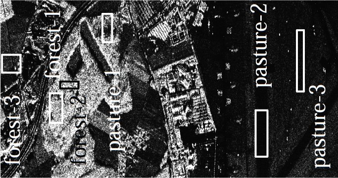
Figure 2: E-SAR image (HH channel) with selected regions.

TABLE I: Parameter estimates

Region	$\widehat{L}$		$|\widehat{\bm{\Sigma}}|$		# pixels
pasture-1	2.	870	7.	934	2106
pasture-2	2.	573	74.	660	2352
pasture-3	2.	889	26.	452	3340
forest-1	2.	638	33615.	990	2870
forest-2	2.	727	10755.	870	2496
forest-3	2.	303	7421.	431	1020

Figure 3 depicts empirical densities of data samples from the selected forest and pasture regions. Additionally, the associated fitted marginal densities are also shown for comparison. In this case, the Wishart density collapses to gamma marginal densities, as demonstrated in (Hagedorn et al., 2006):

$$f_{Z_{i}}(Z^{\prime}_{i};2\sigma^{2}_{i},L)=\frac{{Z^{\prime}_{i}}^{L-1}}{2^{L}\sigma^{2L}_{i}\Gamma(L)}\exp\{-Z^{\prime}_{i}/2\sigma^{2}_{i}\},$$

where $\sigma^{2}_{i}$ is the element $(i,i)$ of $\bm{\Sigma}$, $p=3$, and $Z^{\prime}_{i}$ is the entry $(i,i)$ of the random matrix $\bm{Z}$, and $1\leq i\leq 3$ with the association $1$ to HH, $2$ to HV and $3$ to VV. The adequacy of the model to the data is noteworthy. These samples will be used to validate our proposed methods in Section IV.

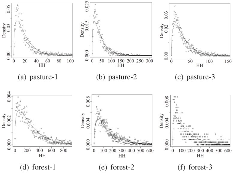
Figure 3: Histograms and empirical densities of samples.

III Statistical information theory for random matrices

In the following we adhere to the convention that a (stochastic) ‘divergence’ is any non-negative function of two probability measures. If the function is also symmetric, it is called a (stochastic) ‘distance’. Finally, we understand (stochastic) ‘metric’ as a distance which satisfies the triangular inequality (Deza and Deza, 2009, chapters 1 and 14).

An image can be understood as a set of regions formed by pixels which are observations of random variables following a certain distribution. Therefore, stochastic dissimilarity measures could be used as features within image analysis techniques, since they may be able to assess the difference between the distributions that describe different image areas (Nascimento et al., 2010). Dissimilarity measures were submitted to a systematic and comprehensive treatment in (Ali and Silvey, 1996; Csiszár, 1967; Salicrú et al., 1994) and, as a result, the class of $(h,\phi)$-divergences was proposed (Salicrú et al., 1994).

Assume that $\bm{X}$ and $\bm{Y}$ are random matrices whose distributions are characterized by the densities $f_{\bm{X}}(\bm{Z}^{\prime};\bm{\theta}_{1})$ and $f_{\bm{Y}}(\bm{Z}^{\prime};\bm{\theta}_{2})$, respectively, where $\bm{\theta}_{1}$ and $\bm{\theta}_{2}$ are parameters. Both densities are assumed to share a common support given by the cone of Hermitian positive definite matrices $\bm{\mathcal{A}}$. The $(h,\phi)$-divergence between $f_{\bm{X}}$ and $f_{\bm{Y}}$ is defined by

$$D_{\phi}^{h}(\bm{X},\bm{Y})=h\biggl{(}\int_{\bm{\mathcal{A}}}\phi\Big{(}\frac{f_{\bm{X}}(\bm{Z}^{\prime};\bm{\theta}_{1})}{f_{\bm{Y}}(\bm{Z}^{\prime};\bm{\theta}_{2})}\Big{)}f_{\bm{Y}}(\bm{Z}^{\prime};\bm{\theta}_{2})\mathrm{d}\bm{Z}^{\prime}\biggr{)},$$ (14)

where $\phi\colon(0,\infty)\rightarrow[0,\infty)$ is a convex function and $h\colon(0,\infty)\rightarrow[0,\infty)$ is a strictly increasing function with $h(0)=0$. The differential element $\mathrm{d}\bm{Z}^{\prime}$ is given by

$$\mathrm{d}\bm{Z}^{\prime}=\mathrm{d}Z^{\prime}_{11}\mathrm{d}Z^{\prime}_{22}\cdots\mathrm{d}Z^{\prime}_{pp}\displaystyle\prod^{p}_{\underbrace{i,j=1}_{i<j}}\mathrm{d}\Re\{Z^{\prime}_{ij}\}\mathrm{d}\Im\{Z^{\prime}_{ij}\},$$

where $Z^{\prime}_{ij}$ is the $(i,j)$ entry of matrix $\bm{Z}^{\prime}$, and operators $\Re\{\cdot\}$ and $\Im\{\cdot\}$ return real and imaginary parts of their arguments, respectively (Goodman, 1963). If indeterminate forms appear in (14) due to the ratio of densities, they are assigned value zero.

Well-known divergences arise with adequate choices of $h$ and $\phi$. Among them, the following were examined: (i) the $\chi^{2}$ divergence (Taneja, 2006), (ii) the Kullback-Leibler divergence (Seghouane and Amari, 2007), (iii) the Rényi divergence (Rached et al., 2001), (iv) the Bhattacharyya distance (Kailath, 1967), and (v) the Hellinger distance (Nascimento et al., 2010). As the triangular inequality is not necessarily satisfied, not every divergence measures is a metric (Burbea and Rao, 1982). Additionally, the symmetry property is not followed by some of these divergence measures. However, such tools are mathematically appropriated for comparing the distribution of random variables (Aviyente, 2003). Thus, the following expression has been suggested as a possible solution for this problem (Seghouane and Amari, 2007):

$$d_{\phi}^{h}(\bm{X},\bm{Y})=\frac{D_{\phi}^{h}(\bm{X},\bm{Y})+D_{\phi}^{h}(\bm{Y},\bm{X})}{2}.$$

In analogy with Goudail and Réfrégier (2004); Morio et al. (2008), this paper defines distances as symmetrized versions of the divergence measures, i.e., a function $d_{\phi}^{h}:\bm{\mathcal{A}}\times\bm{\mathcal{A}}\rightarrow\mathbbm{R}$ is a distance on $\bm{\mathcal{A}}$ if, for all $\bm{X},\bm{Y}\in\bm{\mathcal{A}}$, the following properties holds:

1. Non-negativity: $d_{\phi}^{h}(\bm{X},\bm{Y})\geq 0$.

2. Symmetry: $d_{\phi}^{h}(\bm{X},\bm{Y})=d_{\phi}^{h}(\bm{Y},\bm{X})$.

3. Identity of indiscernibles: $d_{\phi}^{h}(\bm{X},\bm{Y})=0\Leftrightarrow\bm{X}=\bm{Y}$.

Thus, the $\chi^{2}$, Kullback-Leibler, and Rényi divergences were made symmetric distances. Table II shows the functions $h$ and $\phi$ which lead to each of the above listed distances.

TABLE II: ($h,\phi$)-distance and related functions $\phi$ and $h$

$(h,\phi)$-distance	$h(y)$	$\phi(x)$
$\chi^{2}$	$y/4$	$(x-1)^{2}(x+1)/x$
Kullback-Leibler	${y}/{2}$	$(x-1)\log x$
Rényi (order $\beta$)	$\frac{1}{\beta-1}\log((\beta-1)y+1),\;0\leq y<\frac{1}{1-\beta}$	$\frac{x^{1-\beta}+x^{\beta}-\beta(x-1)-2}{2(\beta-1)},0<\beta<1$
Bhattacharyya	$-\log(1-y),0\leq y<1$	$-\sqrt{x}+\frac{x+1}{2}$
Hellinger	${y}/{2},0\leq y<2$	$(\sqrt{x}-1)^{2}$

In the following we discuss integral expressions of these $(h,\phi)$-distances. For simplicity, we suppress the explicit dependence on $\bm{Z}^{\prime}$ and on the support $\bm{\mathcal{A}}$.

1. The $\chi^{2}$ distance:

   $$d_{\chi^{2}}(\bm{X},\bm{Y})=\frac{1}{2}[D_{\chi^{2}}(\bm{X},\bm{Y})+D_{\chi^{2}}(\bm{Y},\bm{X})]=\frac{1}{2}\Big{[}\int\frac{(f_{\bm{X}}-f_{\bm{Y}})^{2}}{2f_{\bm{X}}}+\int\frac{(f_{\bm{X}}-f_{\bm{Y}})^{2}}{2f_{\bm{Y}}}\Big{]}.$$

   The divergence $D_{\chi^{2}}$ has been used in many statistical contexts. For instance, Broniatowski and Keziou (2009) proposed efficient hypothesis test combining it with the duality technique.

2. The Kullback-Leibler distance:

   $$d_{\text{KL}}(\bm{X},\bm{Y}) =\frac{1}{2}[D_{\text{KL}}(\bm{X},\bm{Y})+D_{\text{KL}}(\bm{Y},\bm{X})]=\frac{1}{2}\biggl{[}\int f_{\bm{X}}\log{\frac{f_{\bm{X}}}{f_{\bm{Y}}}}+\int f_{\bm{Y}}\log{\frac{f_{\bm{Y}}}{f_{\bm{X}}}}\biggl{]}$$

   $$=\frac{1}{2}\int(f_{\bm{X}}-f_{\bm{Y}})\log{\frac{f_{\bm{X}}}{f_{\bm{Y}}}}.$$

   The divergence $D_{\text{KL}}$ has a close relationship with the Neymman-Pearson lemma (Eguchi and Copas, 2006) and its symmetrization has been suggested as a correction form of the Akaike information criterion, which is a descriptive measure for assessing the adequacy of statistical models.

3. The Rényi distance of order $\beta$:

   $$\widetilde{d_{\text{R}}^{\beta}}(\bm{X},\bm{Y})=\frac{1}{2}[D_{\text{R}}^{\beta}(\bm{X},\bm{Y})+D_{\text{R}}^{\beta}(\bm{Y},\bm{X})]=\frac{\log\int f_{\bm{X}}^{\beta}f_{\bm{Y}}^{1-\beta}+\log\int f_{\bm{X}}^{1-\beta}f_{\bm{Y}}^{\beta}}{2(\beta-1)},$$

   where $0<\beta<1$. The divergence $D_{\text{R}}^{\beta}$ has been used for analysing geometric characteristics with respect to probability laws (Andai, 2009). By the Fejer inequality (Neuman, 1990), we have that

   $${d_{\text{R}}^{\beta}}(\bm{X},\bm{Y})\triangleq\frac{1}{\beta-1}\log\frac{\int f_{\bm{X}}^{\beta}f_{\bm{Y}}^{1-\beta}+\int f_{\bm{X}}^{1-\beta}f_{\bm{Y}}^{\beta}}{2}\leq\widetilde{d_{\text{R}}^{\beta}}(\bm{X},\bm{Y}).$$

   Being ${d_{\text{R}}^{\beta}}$ more tractable than $\widetilde{d_{\text{R}}^{\beta}}$ for algebraic manipulation with the scaled multilook complex Wishart density, this paper will consider the former.

4. The Bhattacharyya distance:

   $$d_{\text{B}}(\bm{X},\bm{Y})=-\log\int\sqrt{f_{\bm{X}}f_{\bm{Y}}}.$$

   Goudail et al. showed that this distance is an efficient tool for contrast definition in algorithms for image processing (Goudail et al., 2004).

5. The Hellinger distance:

   $$d_{\text{H}}(\bm{X},\bm{Y})=1-\int\sqrt{f_{\bm{X}}f_{\bm{Y}}}.$$

   Estimation methods based on the minimization of $d_{\text{H}}$ have been successfully employed in the context of stochastic differential equations (Giet and Lubrano, 2008).

When considering the distance between particular cases of the same distribution, only the parameters are relevant. In this case, the parameters $\bm{\theta}_{1}$ and $\bm{\theta}_{2}$ replace the random variables $\bm{X}$ and $\bm{Y}$. This notation is in agreement with that of Salicrú et al. (1994).

In the following five subsections, we present the expressions of the discussed distances for the scaled multilook complex Wishart distribution, characterized by the density given in equation (1) are presented.

III-A Stochastic distances between scaled multilook complex Wishart laws

In the following subsections, analytic expressions for the stochastic distances $d_{\chi^{2}}$, $d_{\text{KL}}$, $d_{\text{R}}^{\beta}$, $d_{\text{B}}$, and $d_{\text{H}}$ between two complex scaled multilook complex Wishart distributions are presented. In all instances, the parameters $\bm{\theta}_{X}=(L_{X},\bm{\Sigma}_{X})$ and $\bm{\theta}_{Y}=(L_{Y},\bm{\Sigma}_{Y})$ were considered. In order to avoid confusion with the determinant, the absolute value of the scalar $x$ will be denoted $\operatorname{abs}(x)$.

III-A1 the $\chi^{2}$ distance

$$d_{\chi^{2}}(\bm{\theta}_{X},\bm{\theta}_{Y})=\frac{I_{XY}^{\chi^{2}}+I_{YX}^{\chi^{2}}-2}{4},$$

where

$$I_{ij}^{\chi^{2}}= \frac{|\bm{\Sigma}_{i}|^{L_{i}}}{|\bm{\Sigma}_{j}|^{2L_{j}}}\operatorname{abs}(|(2L_{j}\bm{\Sigma}_{j}^{-1}-L_{i}\bm{\Sigma}_{i}^{-1})^{-1}|)^{\operatorname{abs}(2L_{j}-L_{i})} \frac{L_{i}^{-pL_{i}}}{L_{j}^{-2pL_{j}}}\prod_{k=1}^{p-1}\frac{(L_{i}-k)^{k}}{(L_{j}-k)^{2k}}\operatorname{abs}(2L_{j}-L_{i}-k)^{k}$$

$$\bigg{[}\frac{\Gamma(L_{i}-p+1)\Gamma(\operatorname{abs}(2L_{j}-L_{i}-p+1))}{\Gamma(L_{j}-p+1)^{2}}\bigg{]}^{p}$$

for $(i,j)\in\{(X,Y),(Y,X)\}$.

III-A2 The Kullback-Leibler distance

$$d_{\text{KL}}(\bm{\theta}_{X},\bm{\theta}_{Y})= \frac{L_{X}-L_{Y}}{2}\biggl{\{}\log\frac{|\bm{\Sigma}_{X}|}{|\bm{\Sigma}_{Y}|}+p\bigl{[}\psi^{(0)}(L_{X}-p+1)-\psi^{(0)}(L_{Y}-p+1)\bigr{]}$$

$$-p\log\frac{L_{X}}{L_{Y}}+(L_{Y}-L_{X})\sum_{i=1}^{p-1}\frac{i}{(L_{X}-i)(L_{Y}-i)}\biggr{\}}-\frac{p(L_{X}+L_{Y})}{2}$$

$$+\frac{\operatorname{tr}(L_{Y}\bm{\Sigma}_{Y}^{-1}\bm{\Sigma}_{X}+L_{X}\bm{\Sigma}_{X}^{-1}\bm{\Sigma}_{Y})}{2}.$$

III-A3 The Rényi distance of order $\beta$

$$d_{\text{R}}^{\beta}(\bm{\theta}_{X},\bm{\theta}_{Y})=\frac{1}{\beta-1}\log\frac{I(\bm{\theta}_{X},\bm{\theta}_{Y})}{2},$$

such that

$$I(\bm{\theta}_{X},\bm{\theta}_{Y})=$$

$$\Bigl{[}\Gamma(L_{X}-p+1)^{p}|\bm{\Sigma}_{X}|^{L_{X}}L_{X}^{-pL_{X}}\displaystyle\prod_{i=1}^{p-1}(L_{X}-i)^{i}\Bigr{]}^{-\beta}\Bigl{[}\Gamma(L_{Y}-p+1)^{p}|\bm{\Sigma}_{Y}|^{L_{Y}}L_{Y}^{-pL_{Y}}\displaystyle\prod_{i=1}^{p-1}(L_{Y}-i)^{i}\Bigr{]}^{\beta-1}$$

$$\Gamma(E_{1}-p+1)^{p}|\bm{\Sigma}_{XY}|^{E_{1}}\displaystyle\prod_{i=1}^{p-1}(E_{1}-i)^{i}+\Bigl{[}(\Gamma(L_{X}-p+1)^{p}|\bm{\Sigma}_{X}|^{L_{X}}L_{X}^{-pL_{X}}\displaystyle\prod_{i=1}^{p-1}(L_{X}-i)^{i}\Bigr{]}^{\beta-1}$$

$$\Bigl{[}\Gamma(L_{Y}-p+1)^{p}|\bm{\Sigma}_{Y}|^{L_{Y}}L_{Y}^{-pL_{Y}}\displaystyle\prod_{i=1}^{p-1}(L_{Y}-i)^{i}\Bigr{]}^{-\beta}\Gamma(E_{2}-p+1)^{p}|\bm{\Sigma}_{YX}|^{E_{2}}\displaystyle\prod_{i=1}^{p-1}(E_{2}-i)^{i},$$

where $E_{1}=\beta L_{X}+(1-\beta)L_{Y},\;E_{2}=\beta L_{Y}+(1-\beta)L_{X}$, $0<\beta<1$, and $\bm{\Sigma}_{ij}=|(L_{i}\beta\bm{\Sigma}_{i}^{-1}+L_{j}(1-\beta)\bm{\Sigma}_{j}^{-1})^{-1}|$ for $(i,j)\in\{(X,Y),(Y,X)\}$.

III-A4 The Bhattacharyya distance

$$d_{\text{B}}(\bm{\theta}_{X},\bm{\theta}_{Y}) =\sum_{k=0}^{p-1}\log\frac{\sqrt{\Gamma(L_{X}-k)\Gamma(L_{Y}-k)}}{\Gamma(\frac{L_{X}+L_{Y}}{2}-k)}+\frac{L_{X}\log|\bm{\Sigma}_{X}|}{2}+\frac{L_{Y}\log|\bm{\Sigma}_{Y}|}{2}$$

$$-\frac{p}{2}\bigl{(}L_{X}\log{L_{X}}+L_{Y}\log{L_{Y}}\bigr{)}-\frac{L_{X}+L_{Y}}{2}\log\biggl{|}\biggl{(}\frac{L_{X}\bm{\Sigma}_{X}^{-1}+L_{Y}\bm{\Sigma}_{Y}^{-1}}{2}\biggr{)}^{-1}\biggr{|}.$$

III-A5 The Hellinger distance

$$d_{\text{H}}(\bm{\theta}_{X},\bm{\theta}_{Y})=1-\frac{\Bigl{|}\Bigl{(}\frac{L_{X}\bm{\Sigma}_{X}^{-1}+L_{Y}\bm{\Sigma}_{Y}^{-1}}{2}\Bigr{)}^{-1}\Bigr{|}^{\frac{L_{X}+L_{Y}}{2}}}{|\bm{\Sigma}_{X}|^{\frac{L_{X}}{2}}|\bm{\Sigma}_{Y}|^{\frac{L_{Y}}{2}}}\sqrt{L_{X}^{pL_{X}}L_{Y}^{pL_{Y}}}\prod_{k=0}^{p-1}\frac{\Gamma\bigl{(}\frac{L_{X}+L_{Y}}{2}-k\bigr{)}}{\sqrt{\Gamma(L_{X}-k)\Gamma(L_{Y}-k)}}$$

III-A6 Sensitivity analysis

Now we examine the behavior of the distances with respect to the variation of parameters. First, we assume a fixed number of looks, namely $L=8$, and adopt the following parameters: $\bm{\theta}_{1}=(8,\bm{\Sigma}(360932))$ and $\bm{\theta}_{2}=(8,\bm{\Sigma}(x))$, where

$$\bm{\Sigma}(x)={\left[\begin{array}[]{ccc}x&11050+3759\textbf{i}&63896+1581\textbf{i}\\ &98960&6593+6868\textbf{i}\\ &&208843\end{array}\right]}.$$

As the covariance matrix is Hermitian, only the upper triangle and the diagonal are displayed. The fixed covariance matrix $\bm{\Sigma}(360932)$ was observed by Frery et al. (2010) in PolSAR data of forested areas.

Figure 4(a) shows the distances for $x\in[359000,363000]$. The three uppermost curves, i.e., the ones that vary more abruptly, are $d_{\chi^{2}}$ and $d_{\text{KL}}$, which are overlapped, and $d_{\text{R}}^{0.9}$. Analogously, distances $d_{\text{B}}$ and $d_{\text{H}}$ present roughly the same behavior and are also superimposed. The least varying distance is $d_{\text{R}}^{0.1}$.

We also considered fixed covariance matrices with varying number of looks: $\bm{\theta}_{1}=(8,\bm{\Sigma}(360932))$ and $\bm{\theta}_{2}=(m,\bm{\Sigma}(360932))$, for $5\leq m\leq 11$. Figure 4(b) shows the distances, where we notice that $d_{\text{KL}}$ is the one that varies most, followed by $d_{\chi^{2}}$, $d_{\text{R}}^{0.9}$, $d_{\text{B}}$, $d_{\text{H}}$, and $d_{\text{R}}^{0.1}$.

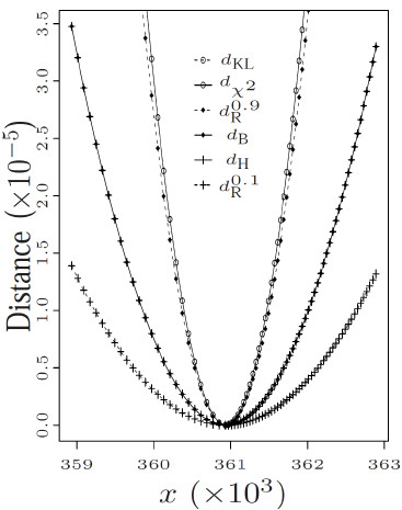
(a) Varying $\bm{\Sigma}$

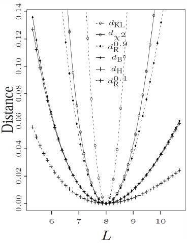
(b) Varying $L$

Figure 4: Sensitivity of the proposed distances.

It is noteworthy that the distances are much more sensitive to variations of one element of the covariance matrix than to variations of the number of looks.

As presented by Yu et al. (2008), in order to make fair comparisons among stochastic distances, the distributions must be indexed by the same parameter. The evidence presented in Fig. 4 strongly suggests that $d_{\chi^{2}}$, $d_{\text{KL}}$, and $d_{\text{R}}^{0.9}$ outperform all other distances. This is due to their higher sensitivity to variations around fixed parameter values, that makes them more suitable for discrimination purposes.

III-B Hypothesis test based on divergence for positive-definite Hermitian data

In the following, the hypothesis test based on stochastic distances proposed by Salicrú et al. (1994) are recalled and applied to scaled multilook complex Wishart laws.

Let $\widehat{\bm{\theta}}_{1}=(\widehat{\theta}_{11},\ldots,\widehat{\theta}_{1M})$ and $\widehat{\bm{\theta}}_{2}=(\widehat{\theta}_{21},\ldots,\widehat{\theta}_{2M})$ be the ML estimators of parameters $\bm{\theta}_{1}$ and $\bm{\theta}_{2}$ based on independent samples of size $N_{X}$ and $N_{Y}$, respectively. Under the regularity conditions discussed by Salicrú et al. (1994, p. 380) the following lemma holds:

Lemma 1

If $\frac{N_{X}}{N_{X}+N_{Y}}\xrightarrow[N_{X},N_{Y}\rightarrow\infty]{}\lambda\in(0,1)$ and $\bm{\theta}_{1}=\bm{\theta}_{2}$, then

$$S_{\phi}^{h}(\widehat{\bm{\theta}}_{1},\widehat{\bm{\theta}}_{2})=\frac{2N_{X}N_{Y}}{N_{X}+N_{Y}}\frac{d^{h}_{\phi}(\widehat{\bm{\theta}}_{1},\widehat{\bm{\theta}}_{2})}{h{{}^{\prime}}(0)\phi{{}^{\prime\prime}}(1)}\xrightarrow[N_{X},N_{Y}\rightarrow\infty]{\mathcal{D}}\chi_{M}^{2},$$

where “$\xrightarrow[]{\mathcal{D}}$” denotes convergence in distribution.

Based on Lemma 1, statistical hypothesis tests for the null hypothesis $\bm{\theta}_{1}=\bm{\theta}_{2}$ can be derived in the form of following proposition.

Proposition 1

Let $N_{X}$ and $N_{Y}$ be large and $S_{\phi}^{h}(\widehat{\bm{\theta}}_{1},\widehat{\bm{\theta}}_{2})=s$, then the null hypothesis $\bm{\theta}_{1}=\bm{\theta}_{2}$ can be rejected at level $\alpha$ if $\Pr(\chi^{2}_{M}>s)\leq\alpha$.

We denote the statistics based on the Kullback-Leibler, Bhattacharya, Hellinger, Rényi, and chi-square distances as $S_{\text{KL}},S_{\text{B}},S_{\text{H}},S_{\text{R}}^{\beta}$, and $S_{\chi^{2}}$, respectively.

IV Simulation and application

This section reports the assessment of the proposed methods as contrast measures. Both synthetic and actual image data are considered. Moreover, a robustness analysis was performed in order to characterize the behavior of such measures in the presence of outliers.

IV-A Synthetic data analysis

We assess the influence of estimation on the size of the new hypothesis tests using simulated data. The study is conducted sampling from $L=L_{X}=L_{Y}\in\{4,8,16\}$ looks and from each of the covariance matrices observed in the forest areas presented in Figure 3. The sample sizes represent square windows of size $7\times 7$, $11\times 11$, and $20\times 20$ pixels, i.e., $N_{X},N_{Y}\in\{49,121,400\}$, which are typical in image processing and analysis. Nominal significance levels $\alpha\in\{1\%,5\%\}$ are verified.

Let $T$ be the number of Monte Carlo replicas and $C$ the number of cases for which the null hypothesis is rejected at nominal level $\alpha$ when samples come from the same distribution. The empirical test size is given by $\widehat{\alpha}_{1-\alpha}={C}/{T}$ . Following the methodology described by Nascimento et al. (2010), we used $T=5500$ replicas.

Table III presents the empirical test size at $1\%$ and $5\%$ nominal levels, the execution time in miliseconds, and the distances mean ($\overline{d}$) and coefficient of variation (CV). The smallest empirical size and distance mean are in boldface.

TABLE III: Empirical sizes for forest-1

Factors			$L=4$					$L=8$					$L=16$
$S_{\phi}^{h}$	$N_{X}$	$N_{Y}$	$1\%$	$5\%$	time (ms)	$\overline{d}$	CV	$1\%$	$5\%$	time (ms)	$\overline{d}$	CV	$1\%$	$5\%$	time (ms)	$\overline{d}$	CV
$S_{\chi^{2}}$	49	49	84.96	91.55	1.03	64.58	159.51	81.55	89.13	1.08	52.62	81.55	78.69	87.05	1.09	48.70	78.16
	49	121	82.44	90.62	1.11	50.74	86.63	78.98	88.07	1.08	44.90	68.93	76.64	86.64	1.07	42.26	65.09
	49	400	81.84	90.38	1.02	47.40	66.63	77.09	87.64	1.09	42.84	63.52	74.93	85.11	1.06	40.71	61.99
	121	121	79.96	89.27	1.07	43.89	60.13	76.16	86.58	1.09	40.16	59.26	73.76	85.31	1.04	38.12	57.44
	121	400	78.78	88.51	1.12	41.76	56.54	74.25	85.53	1.08	37.16	54.32	73.33	84.84	1.12	37.26	56.76
	400	400	77.96	87.60	1.09	38.88	52.01	73.36	84.71	1.05	35.95	51.72	71.51	83.56	1.10	34.99	51.39
$S_{\text{KL}}$	49	49	1.91	7.18	0.44	10.59	45.65	1.05	4.85	0.49	9.75	46.78	0.91	4.22	0.39	9.39	47.80
	49	121	1.58	6.35	0.41	10.47	45.78	1.00	4.42	0.45	9.60	46.02	0.78	3.67	0.45	9.24	46.92
	49	400	1.56	6.95	0.48	10.57	45.02	1.04	4.35	0.46	9.67	46.36	0.82	3.95	0.47	9.32	47.49
	121	121	1.67	6.62	0.43	10.56	45.79	0.85	4.60	0.49	9.66	46.80	0.75	3.78	0.48	9.21	47.09
	121	400	1.82	7.64	0.50	10.69	45.69	0.76	4.27	0.46	9.49	45.90	1.16	4.49	0.47	9.43	48.43
	400	400	1.47	6.91	0.42	10.55	44.91	1.00	4.16	0.50	9.58	46.21	0.58	3.56	0.46	9.26	46.46
$S_{\text{R}}^{\beta}$	49	49	5.89	14.76	1.10	12.38	49.66	4.13	12.93	1.12	11.72	50.22	4.20	11.40	1.07	11.35	51.15
	49	121	4.78	14.38	1.00	12.18	49.79	3.89	11.58	1.10	11.52	49.94	3.62	10.36	1.09	11.16	50.18
	49	400	5.71	15.18	1.08	12.31	49.25	4.25	12.47	0.96	11.62	50.38	3.85	11.11	1.11	11.27	50.84
	121	121	5.56	14.69	1.11	12.32	49.56	4.07	12.02	0.99	11.59	50.65	3.45	10.71	1.12	11.17	50.14
	121	400	6.29	16.00	1.11	12.47	50.31	3.65	11.20	1.06	11.33	49.50	3.98	11.36	1.01	11.40	51.57
	400	400	5.71	15.24	0.99	12.35	49.47	3.69	11.62	1.13	11.50	49.55	3.27	11.35	1.20	11.23	49.49
$S_{\text{B}}$	49	49	5.51	14.25	0.54	12.27	49.22	3.96	12.65	0.51	11.66	50.01	4.07	11.31	0.58	11.33	51.04
	49	121	4.56	14.04	0.65	12.10	49.48	3.78	11.35	0.51	11.48	49.80	3.58	10.29	0.57	11.14	50.11
	49	400	5.45	14.84	0.56	12.25	49.01	4.18	12.36	0.57	11.59	50.26	3.84	11.02	0.58	11.26	50.78
	121	121	5.42	14.47	0.57	12.27	49.39	3.98	11.95	0.61	11.56	50.56	3.45	10.64	0.56	11.16	50.09
	121	400	6.20	15.75	0.56	12.44	50.20	3.62	11.09	0.55	11.32	49.44	3.98	11.36	0.51	11.40	51.54
	400	400	5.65	15.18	0.57	12.33	49.42	3.67	11.58	0.57	11.50	49.52	3.27	11.33	0.65	11.23	49.47
$S_{\text{H}}$	49	49	4.20	11.93	0.53	11.80	47.24	2.93	10.36	0.56	11.24	48.11	2.78	9.11	0.54	10.93	49.10
	49	121	3.73	12.29	0.50	11.78	48.01	3.00	10.05	0.52	11.20	48.41	2.87	9.27	0.60	10.87	48.80
	49	400	4.49	13.38	0.64	11.99	47.90	3.56	10.93	0.62	11.36	49.16	3.27	9.71	0.55	11.04	49.72
	121	121	4.89	13.58	0.58	12.08	48.56	3.60	11.35	0.62	11.39	49.77	2.96	9.87	0.62	11.00	49.34
	121	400	5.67	15.18	0.60	12.31	49.64	3.35	10.58	0.54	11.22	48.96	3.71	10.80	0.60	11.29	50.99
	400	400	5.40	14.93	0.55	12.27	49.17	3.51	11.38	0.51	11.44	49.29	3.11	11.02	0.58	11.18	49.26

Average distances reduce when the number of looks increases, i.e., improving image quality corrects the statistics in terms of test size. With the exception of the $\chi^{2}$ distance, these distances vary in the interval ($45.02,51.54$) regardless the sample sizes. Fixing the sample sizes while varying the number of looks $L$, the test sizes obey the inequalities $S_{\text{KL}}\leq S_{\text{H}}\leq S_{\text{B}}\leq S_{\text{R}}^{\beta}\leq S_{\chi^{2}}$.

The test based on the Kullback-Leibler distance presented the best performance in terms of both empirical test size and execution time. The other tests showed poorer performance, even with large samples and high number of looks. Small samples or number of looks yield poor tests, and the test based on the $\chi^{2}$ distance is unacceptable.

IV-B Image data analysis

The methodology for assessing test size presented in Section III-B was applied to the three forest samples of the E-SAR image presented in Figure 2. Each sample was submitted to the following procedure (Nascimento et al., 2010):

1. partition the sample in disjoint blocks of size $N_{X}$;

2. for each block from (b1), split the remaining sample in disjoint blocks of size $N_{Y}$;

3. perform the hypothesis test as described in Proposition 1 for each pair of samples with sizes $N_{X}$ and $N_{Y}$.

Table IV presents the results. Except for the test based on the $\chi^{2}$ distance, all test sizes were smaller than the nominal level; i.e., the tests did not reject the null hypothesis when it is true. Although $S_{\chi^{2}}$ presented the worst performance in general, it is equal to zero when $N_{X}=N_{Y}=400$, showing the importance of the sample size on the test size.

TABLE IV: Empirical sizes for forests

Factors			forest-1				forest-2				forest-3
$S_{\phi}^{h}$	$N_{X}$	$N_{Y}$	$1\%$	$5\%$	$\overline{d}\;(\times 10^{-1})$	CV	$1\%$	$5\%$	$\overline{d}\;(\times 10^{-1})$	CV	$1\%$	$5\%$	$\overline{d}\;(\times 10^{-1})$	CV
$S_{\chi^{2}}$	49	49	49.30	53.06	$\text{10}^{\text{25}}$	4065.70	55.27	58.37	$\text{10}^{\text{37}}$	4000.00	61.05	63.16	$\approx\text{10}^{\text{47}}$	1378.40
	49	121	37.77	40.06	$\text{10}^{\text{17}}$	1565.32	43.76	46.42	$\text{10}^{\text{19}}$	2169.27	51.40	52.78	$\text{10}^{\text{7}}\;$	642.51
	49	400	27.12	29.38	$\text{10}^{\text{11}}$	1330.26	29.77	29.77	$\text{10}^{\text{27}}$	1144.55	43.75	43.75	$\text{10}^{\text{9}}\;$	396.99
	121	121	14.62	16.60	$\text{10}^{\text{7}}\;$	1197.95	24.21	30.00	$\text{10}^{\text{21}}$	1378.40	46.43	50.00	$\text{10}^{\text{8}}\;$	446.32
	121	400	5.80	5.80	137.97	603.05	7.84	11.76	68.36	169.33	40.00	40.00	494.91	179.09
	400	400	0.00	0.00	12.16	77.12	0.00	0.00	2.74	39.25	0.00	0.00	6.54	$-$
$S_{\text{KL}}$	49	49	0.00	0.00	17.63	56.82	0.00	0.00	15.63	47.24	0.00	0.00	46.73	57.31
	49	121	0.00	0.00	10.91	56.50	0.00	0.00	10.45	47.29	0.00	0.00	30.12	62.51
	49	400	0.00	0.00	7.81	60.15	0.00	0.00	7.47	46.14	0.00	0.00	18.07	73.62
	121	121	0.00	0.00	7.09	44.14	0.00	0.00	8.02	54.38	0.00	0.00	29.83	53.86
	121	400	0.00	0.00	4.27	47.16	0.00	0.00	5.28	60.25	0.00	0.00	8.15	52.58
	400	400	0.00	0.00	2.95	38.16	0.00	0.00	16.99	59.64	0.00	0.00	2.61	$-$
$S_{\text{R}}^{\beta}$	49	49	0.00	0.00	13.03	55.22	0.00	0.00	12.15	46.99	0.00	0.00	33.43	55.64
	49	121	0.00	0.00	5.39	55.23	0.00	0.00	5.35	47.13	0.00	0.00	14.47	59.66
	49	400	0.00	0.00	1.67	58.44	0.00	0.00	1.66	45.26	0.00	0.00	3.77	70.50
	121	121	0.00	0.00	5.38	44.49	0.00	0.00	5.97	49.79	0.00	0.00	20.83	52.79
	121	400	0.00	0.00	1.82	45.58	0.00	0.00	2.18	52.40	0.00	0.00	3.46	50.49
	400	400	0.00	0.00	2.12	39.97	0.00	0.00	2.93	37.87	0.00	0.00	1.50	$-$
$S_{\text{B}}$	49	49	0.00	0.00	13.55	50.80	0.00	0.00	12.84	44.45	0.00	0.00	31.06	46.92
	49	121	0.00	0.00	6.67	52.27	0.00	0.00	6.66	45.08	0.00	0.00	16.18	51.24
	49	400	0.00	0.00	3.22	56.22	0.00	0.00	3.20	43.69	0.00	0.00	6.79	63.46
	121	121	0.00	0.00	5.89	43.27	0.00	0.00	6.51	48.77	0.00	0.00	20.63	47.05
	121	400	0.00	0.00	2.51	44.55	0.00	0.00	3.00	51.67	0.00	0.00	4.68	49.27
	400	400	0.00	0.00	2.36	39.41	0.00	0.00	3.62	40.78	0.00	0.00	1.67	$-$
$S_{\text{H}}$	49	49	0.00	0.00	11.37	42.69	0.00	0.00	10.92	37.88	0.00	0.00	21.33	32.77
	49	121	0.00	0.00	5.83	46.05	0.00	0.00	5.86	39.78	0.00	0.00	11.91	37.01
	49	400	0.00	0.00	2.87	51.70	0.00	0.00	2.88	39.37	0.00	0.00	5.33	49.21
	121	121	0.00	0.00	5.46	40.04	0.00	0.00	5.97	45.05	0.00	0.00	15.92	35.68
	121	400	0.00	0.00	2.38	42.09	0.00	0.00	2.80	48.53	0.00	0.00	4.22	46.42
	400	400	0.00	0.00	2.29	38.33	0.00	0.00	3.05	38.90	0.00	0.00	1.64	$-$

This analysis reveals that the test based on Kullback-Leibler distance has the best performance with image data. Small test sizes are important in order to prevent oversegmentation, i.e., the erroneous identification of samples from the same class as coming from different targets.

IV-C Kullback-Leibler distance robustness

Limited to the $S_{\text{KL}}$ statistic, the following discussion presents a robustness study of its test size in the presence of outliers. Only one sample in the test will be contaminated, and the contamination model we adopt consists in allowing each observation from this sample to come from a different distribution than the assumed with a small probability.

The uncontaminated sample is formed by observations from the $\mathcal{W}(L,\bm{\Sigma})$ distribution, while the contaminated sample is formed by observations from either this law, with probability $1-\epsilon$, or from $\mathcal{W}(L,1000\bm{\Sigma})$ with probability $\epsilon$; in our study, $\epsilon=10^{-5}$. In other words, the cumulative distribution function of the contaminated sample is given by

$$\epsilon\cdot F_{\bm{X}}(\bm{Z}^{\prime})+(1-\epsilon)\cdot F_{\bm{Y}}(\bm{Z}^{\prime}).$$

Table V shows the empirical test sizes as well as the following additional figures: (c1) the ML estimator mean square error (MSE) for the number of looks, (c2) the relative mean square error (rMSE) for the covariance matrix estimator adapted from the ‘total relative bias’ (Cribari-Neto et al., 2000), (c3) the ratios between mean square errors, and (c4) the distances mean and coefficient of variation.

The mean square error for the number of looks estimation is given by $\operatorname{MSE}(\widehat{L}_{I})=\sum_{k=1}^{5500}(\widehat{L}^{(I)}_{k}-L_{I})^{2}/5500$, where $\widehat{L}^{(I)}_{k}$ represents the obtained estimates at the kth Monte Carlo replication for population $I\in\{X,Y\}$. For the covariance matrix, the relative mean square error is

$$\operatorname{rMSE}(\widehat{\bm{\Sigma}}_{I})=\frac{1}{5500}\sum_{k=1}^{5500}\sum_{h=1}^{3}\frac{((\widehat{\bm{\Sigma}}^{(I)}_{k})_{hh}-(\bm{\Sigma}_{I})_{hh})^{2}}{(\bm{\Sigma}_{I})_{kk}},$$

where $\widehat{\bm{\Sigma}}^{(I)}_{k}$ is the estimate of the covariance matrix at the kth Monte Carlo experiment for the population $I$. The ratios for these measures are denoted by

$$r_{1}=\frac{\operatorname{MSE}(\widehat{L}_{X})}{\operatorname{MSE}(\widehat{L}_{Y})}\text{ and }r_{2}=\frac{\operatorname{rMSE}(\widehat{\bm{\Sigma}}_{X})}{\operatorname{rMSE}(\widehat{\bm{\Sigma}}_{Y})}.$$

TABLE V: Robustness for forest-1. Mean square errors scaled by 100

$N_{X}$	$N_{Y}$	$L$	$1\%$	$5\%$	$\overline{d}$	CV	$\operatorname{MSE}$($\widehat{L}_{X}$)	$\operatorname{MSE}$($\widehat{L}_{Y}$)	$r_{1}$	$\operatorname{rMSE}$($\widehat{\bm{\Sigma}}_{X}$)	$\operatorname{rMSE}$($\widehat{\bm{\Sigma}}_{Y}$)	$r_{2}$
49	49	4	1.82	6.87	10.60	45.48	16.28	18.72	0.87	55.36	55.52	1.00
		8	0.95	4.62	9.73	46.66	14.75	16.96	0.87	27.78	28.21	0.98
		16	0.84	4.07	9.41	47.00	14.13	16.03	0.88	13.70	14.67	0.93
49	121	4	2.09	7.80	10.71	46.06	16.23	17.54	0.93	55.05	23.74	2.32
		8	1.02	4.49	9.64	47.20	14.80	15.41	0.96	27.50	11.96	2.30
		16	0.85	4.07	9.44	46.67	14.40	14.71	0.98	13.50	6.56	2.06
49	400	4	1.67	8.07	10.79	45.20	16.31	16.92	0.96	54.53	7.85	6.94
		8	1.07	5.00	9.77	46.95	14.83	14.76	1.00	27.05	4.41	6.13
		16	0.56	4.09	9.55	45.57	14.21	13.97	1.02	13.74	2.70	5.08
121	121	4	2.04	7.64	10.75	45.86	14.90	17.59	0.85	22.24	23.26	0.96
		8	0.80	4.58	9.72	45.40	13.45	15.44	0.87	10.95	12.22	0.90
		16	0.96	4.44	9.56	46.69	12.87	14.71	0.87	5.60	6.60	0.85
121	400	4	2.15	7.69	10.84	45.84	14.88	16.97	0.88	22.08	7.78	2.84
		8	1.05	4.87	9.88	46.04	13.30	14.75	0.90	11.06	4.41	2.51
		16	1.62	5.44	9.73	48.89	12.86	13.97	0.92	5.52	2.73	2.02
400	400	4	1.93	7.87	10.91	44.79	14.31	16.91	0.85	6.54	7.88	0.83
		8	1.22	5.96	10.12	46.00	12.65	14.71	0.86	3.33	4.40	0.76
		16	1.22	6.27	10.22	46.57	12.17	14.01	0.87	1.70	2.74	0.62

The results presented in Table V reveal that the mean square errors are reduced when larger windows or number of looks are considered. This behavior is expected, since in those cases the signal-to-noise ratio is improved.

For situations where $N_{X}=N_{Y}=N\in\{49,121,400\}$, the mean square errors for the estimators of the number of looks and covariance matrix increase when contamination is introduced. Additionally, increasing the value of $N$ does not significantly affect the ratio $r_{1}$. Simultaneously, ratio $r_{2}$ decreases. This last fact is justified by the contamination model nature, and indicates that the contamination effect on the empirical test size is strongly related to the estimation of the covariance matrix.

Figure 5 plots $S_{\text{KL}}$ in pure and contaminated scenarios. As expected, the contamination effect under $S_{\text{KL}}$ increases when considering situations with larger windows. However, this effect is diminished when $L$ increases.

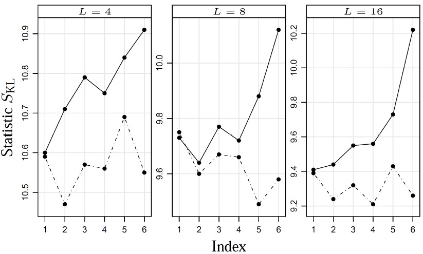
Figure 5: Stochastic distances with $\epsilon=\{0,10^{-5}\}$. For each sample size, scenarios were lexicographically ordered: $[i:(i;N_{X},N_{Y})=\{(1;49,49),$ $(2;49,121),$ $(3;49,400),$ $(4;121,121),$ $(5;121,400),$ $(6;400,400)\}]$.

V Conclusion

This work aimed to provide a statistical formalism for the use of information theory tools in the understanding of PolSAR imagery. Five novel hypothesis tests for polarimetric speckled data were assessed. Their associate statistics were based on chi-square, Kullback-Leibler, Rényi, Bhattacharyya, and Hellinger distances between ML estimators for the parameters that index the scaled multilook complex Wishart law. As a comparison criterion, empirical test sizes were quantified in several situations, which included pure and contaminated data. An application to actual data was performed.

The test based on the Kullback-Leibler distance had the closest empirical size to the nominal level. Under contamination, the ML estimator for the covariance matrix was significantly affected, yielding the $S_{\text{KL}}$ statistic sensitive to outliers. However, this effect was reduced increasing the number of looks, i.e., this contrast measure presented better performance in the presence of contamination when signal-to-noise ratio was controlled. With the exception of the chi-square measure, all stochastic distances presented good performance when applied to a real PolSAR image.

Many venues for research are still open in PolSAR image modelling and analysis. Using stochastic distances in actual segmentation and classification algorithm requires fast and reliable inference procedures which, ideally, are resistant (robust) to plausible contamination. Expressive and tractable models for spatial correlation under the Wishart law, and their implication in inference is another promising research direction. Extending the results here presented to more general models than the scaled multilook complex Wishart law, for instance to the polarimetric $\mathcal{G}^{0}$ and $\mathcal{G}^{H}$ distributions, or even to the still more general complete polarimetric $\mathcal{G}$ model (see Freitas et al., 2005; Frery et al., 2010) would greatly enhance the capability of understanding this class of images.

Afterword

This invited paper is an extended and detailed version of a talk given at the III Simposio de Estadística Espacial y Modelado de Imágenes (SEEMI), that took place at Foz do Iguaçcu, Brazil, in December 2010. Though many results discussed here have been already published in specialized journals and conferences, in this presentation we intend to achieve the wide audience of probability and statistics, with a bias towards applications in signal and image processing.

References

- (1)
- Ali and Silvey (1996) Ali, S. M., Silvey, S. D., 1996. A general class of coefficients of divergence of one distribution from another. Journal of the Royal Statistical Society: Series B (Statistical Methodology), 26, 131–142.
- Andai (2009) Andai, A., 2009. On the geometry of generalized Gaussian distributions. Journal of Multivariate Analysis, 100(4), 777–793.
- Anfinsen et al. (2009) Anfinsen, S. N., Doulgeris, A. P., Eltoft, T., 2009. Estimation of the equivalent number of looks in polarimetric synthetic aperture radar imagery. IEEE Transactions on Geoscience and Remote Sensing, 47(11), 3795–3809.
- Aviyente (2003) Aviyente, S., 2003. Divergence measures for time-frequency distributions. Seventh International Symposium on Signal Processing and Its Applications (SISSPA), 1, 121–124.
- Beaulieu and Touzi (2004) Beaulieu, J. M., Touzi, R., 2004. Segmentation of textured polarimetric SAR scenes by likelihood approximation. IEEE Transactions on Geoscience and Remote Sensing, 42(10), 2063–2072.
- Broniatowski and Keziou (2009) Broniatowski, M., Keziou, A., 2009. Parametric estimation and tests through divergences and the duality technique. Journal of Multivariate Analysis, 100(1), 16–36.
- Burbea and Rao (1982) Burbea, J., Rao, C., 1982. Entropy differential metric, distance and divergence measures in probability spaces: a unified approach. Journal of Multivariate Analysis,12, 575–596.
- Conradsen et al. (2003) Conradsen, K., Nielsen, A. A., Schou, J., Skriver, H., 2003. A test statistic in the complex Wishart distribution and its application to change detection in polarimetric SAR data. IEEE Transactions on Geoscience and Remote Sensing, 41(1), 4–19.
- Cribari-Neto et al. (2000) Cribari-Neto, F., Ferrari, S. L. P., Cordeiro, G. M., 2000. Improved heteroscedasticity-consistent convariance matrix estimators. Biometrika, 87(4), 907–918.
- Csiszár (1967) Csiszár, I., 1967. Information type measures of difference of probability distributions and indirect observations. Studia Scientiarum Mathematicarum Hungarica, 2, 299–318.
- Deza and Deza (2009) Deza, M. M. and Deza, E., 2009. Encyclopedia of Distances, Springer.
- Eguchi and Copas (2006) Eguchi, S., Copas, J., 2006. Interpreting Kullback-Leibler divergence with the Neyman-Pearson lemma. Journal of Multivariate Analysis, 97, 2034–2040.
- Freeman and Durden (1998) Freeman, A., Durden, S. L., 1998. A three-component scattering model for polarimetric SAR data. IEEE Transactions on Geoscience and Remote Sensing, 36(3), 963–973.
- Freitas et al. (2005) Freitas, C. C., Frery, A. C., Correia, A. H., 2005. The polarimetric distribution for SAR data analysis. Environmetrics, 16(1), 13–31.
- Frery et al. (2011) Frery, A. C., Cintra, R. J., Nascimento, A. D. C., 2011. Hypothesis test in complex Wishart distributions. Proceedings of the 5th International Workshop on Science and Applications of SAR Polarimetry and Polarimetric Interferometry (POLinSAR’2011), Frascati, Italy.
- Frery et al. (2010) Frery, A. C., Jacobo-Berlles, J., Gambini, J., Mejail, M., 2010. Polarimetric SAR image segmentation with B-splines and a new statistical model. Multidimensional Systems and Signal Processing, 21, 319–342.
- Gambini et al. (2006) Gambini, J., Mejail, M., Jacobo-Berlles, J., Frery, A. C., 2006. Feature extraction in speckled imagery using dynamic B-spline deformable contours under the G0 model. International Journal of Remote Sensing, 27(22), 5037–5059.
- Gambini et al. (2008) Gambini, J., Mejail, M., Jacobo-Berlles, J., Frery, A. C., 2008. Accuracy of edge detection methods with local information in speckled imagery. Statistics and Computing, 18(1), 15–26.
- Giet and Lubrano (2008) Giet, L., Lubrano, M., 2008. A minimum Hellinger distance estimator for stochastic differential equations: An application to statistical inference for continuous time interest rate models. Computational Statistics & Data Analysis, 52(6), 2945–2965.
- Goodman (1963) Goodman, N. R., 1963. Statistical analysis based on a certain complex Gaussian distribution (an introduction). The Annals of Mathematical Statistics, 34, 152–177.
- Goudail and Réfrégier (2004) Goudail, F., Réfrégier, P., 2004. Contrast definition for optical coherent polarimetric images. IEEE Transactions on Pattern Analysis and Machine Intelligence, 26(7), 947–951.
- Goudail et al. (2004) Goudail, F., Réfrégier, P., Delyon, G., 2004. Bhattacharyya distance as a contrast parameter for statistical processing of noisy optical images. Journal of the Optical Society of America A, 21(7), 1231–1240.
- Hagedorn et al. (2006) Hagedorn, M., Smith, P. J., Bones, P. J., Millane, R. P. and Pairman, D., 2006. A trivariate chi-squared distribution derived from the complex Wishart distribution. Journal of Multivariate Analysis, 97(3), 655–674.
- Hjorungnes and Gesbert (2007) Hjorungnes, A., Gesbert, D., 2007. Complex-valued matrix differentiation: Techniques and key results. IEEE Transactions on Signal Processing, 55(6), 2740–2746.
- Kailath (1967) Kailath, T., 1967. The divergence and Bhattacharyya distance measures in signal selection. IEEE Transactions on Communication Technology, 15, 52–60.
- Kersten et al. (2005) Kersten, P. R., Lee, J. S. and Ainsworth, T. L., 2005. Unsupervised classification of polarimetric synthetic aperture radar images using fuzzy clustering and EM clustering. IEEE Transactions on Geoscience and Remote Sensing, 43(3), 519–527.
- Lee et al. (1994) Lee, J. S. and Hoppel, K. W. and Mango, S. A., Miller, A. R., 1994. Intensity and Phase Statistics of Multilook Polarimetric and Interferometric SAR Imagery. IEEE Transactions on Geoscience and Remote Sensing, 32(5), 1017–1028.
- Lee and Pottier (2009) Lee, J. S., Pottier, E., 2009. Polarimetric Radar Imaging: From Basics to Applications, CRC, Boca Raton.
- Liese and Vajda (2006) Liese, F., Vajda, I., 2006. On divergences and informations in statistics and information theory. IEEE Transactions on Information Theory, 52(10), 4394–4412.
- Lopez-Martinez and Fabregas (2003) Lopez-Martinez, C., Fabregas, X., 2003. Polarimetric SAR speckle noise model. IEEE Transactions on Geoscience and Remote Sensing 41(10), 2232–2242.
- Mak and Barnard (1996) Mak, B., Barnard, E., 1996. Phone clustering using the Bhattacharyya distance. The Fourth International Conference on Spoken Language Processing (ICSLP), 4, Philadelphia, PA, 2005–2008.
- Morio et al. (2008) Morio, J., Réfrégier, P., Goudail, F., Dubois-Fernandez, P. C., Dupuis, X., 2008. Information theory-based approach for contrast analysis in polarimetric and/or interferometric SAR images. IEEE Transactions on Geoscience and Remote Sensing, 46(8), 2185–2196.
- Morio et al. (2009) Morio, J., Réfrégier, P., Goudail, F., Dubois Fernandez, P. C., Dupuis, X., 2009. A characterization of Shannon entropy and Bhattacharyya measure of contrast in polarimetric and interferometric SAR image. Proceedings of the IEEE (PIEEE) 97(6), 1097–1108.
- Nascimento et al. (2010) Nascimento, A. D. C., Cintra, R. J. and Frery, A. C., 2010. Hypothesis testing in speckled data with stochastic distances. IEEE Transactions on Geoscience and Remote Sensing, 48(1), 373–385.
- Neuman (1990) Neuman, E., 1990. Inequalities involving multivariate convex functions II. Proceedings of the American Mathematical Society, 109(4), 965–974.
- Puig and Garcia (2003) Puig, D., Garcia, M. A., 2003. Pixel classification through divergence-based integration of texture methods with conflict resolution. International Conference on Image Processing (ICIP), 3, 1037–1040.
- Rached et al. (2001) Rached, Z., Alajaji, F., Lorne Campbell, L., 2001. Renyi’s divergence and entropy rates for finite alphabet Markov sources. IEEE Transactions on Information Theory, 47(4), 1553–1561.
- Salicrú et al. (1994) Salicrú, M., Menéndez, M. L., Pardo, L., Morales, D., 1994. On the applications of divergence type measures in testing statistical hypothesis. Journal of Multivariate Analysis, 51, 372–391.
- Schou et al. (2003) Schou, J., Skriver, H., Nielsen, A. H., Conradsen, K., 2003. CFAR edge detector for polarimetric SAR images. IEEE Transactions on Geoscience and Remote Sensing, 41(1), 20–32.
- Seghouane and Amari (2007) Seghouane, A. K., Amari, S. I., 2007. The AIC criterion and symmetrizing the Kullback-Leibler divergence. IEEE Transactions on Neural Networks, 18(1), 97–106.
- Taneja (2006) Taneja, I. J., 2006. Bounds on triangular discrimination, harmonic mean and symmetric chi-square divergences. Journal of Concrete and Applicable Mathematics, 4, 91–111.
- Ulaby and Elachi (1990) Ulaby, F. T., Elachi, C., 1990. Radar Polarimetriy for Geoscience Applications, Artech House, Norwood.
- Yu et al. (2008) Yu, J., Amores, J., Sebe, N., Radeva, P., Tian, Q., 2008. Distance learning for similarity estimation. IEEE Transactions on Pattern Analysis and Machine Intelligence, 30(3), 451–462.
- Zografos et al. (1990) Zografos, K., Ferentinos, K., Papaioannou, T., 1990. -divergence statistics: Sampling properties and multinomial goodness-of-fit and divergence tests. Communications in Statistics - Theory Methods, 19, 1785–1802.