Asymptotic safety on the lattice: The Nonlinear O(N) Sigma Model
Abstract
We study the non-perturbative renormalization group flow of the nonlinear O(N) sigma model in two and three spacetime dimensions using a scheme that combines an effective local Hybrid Monte Carlo update routine, blockspin transformations and a Monte Carlo demon method. In two dimensions our results verify perturbative renormalizability. In three dimensions, we determine the flow diagram of the theory for various and different truncations and find a non-trivial fixed point, which indicates non-perturbative renormalizability. It is related to the well-studied phase transition of the O(N) universality class and characterizes the continuum physics of the model. We compare the obtained renormalization group flows with recent investigations by means of the Functional Renormalization Group.
pacs:
11.15.-q, 11.15.Ha, 12.38.AwI Introduction
The renormalization of coupling parameters due to quantum
fluctuations is a characteristic feature of any quantum field theory
and many different methods have been developed to study this
interesting property. While most of these methods rely on a perturbative
treatment of the theories, the investigation of strongly coupled or
strongly correlated systems without small expansion parameter,
like e.g. the theory of strong interaction, requires a
non-perturbative approach. One non-perturbative and very flexible
method is the Functional Renormalization Group (FRG)
introduced by K. Wilson Wilson (1975).
In a particularly useful implementation of the functional renormalization
group, one studies the flow of the effective average action
w.r.t. the momentum scale , which interpolates between the
bare action at the UV-cutoff , and the full effective
action in the IR, Wetterich (1993).
With the help of this powerful non-perturbative approach one can explore
theories which are non-renormalizable in perturbation theory,
i.e. in the vicinity of a Gaußian fixed point,
but are renormalizable in a non-perturbative setting.
In such asymptotically save theories the running of the couplings
in the UV is controlled by a non-trivial fixed point with a finite
number of relevant directions.
The most important theory where this so-called asymptotic safety scenario
of Weinberg Hawking and Israel (1979); Niedermaier and Reuter (2006) could be realized
is general relativity where at present all results suggest that there exists
a non-trivial UV fixed point
Reuter and Saueressig (2002); Benedetti et al. (2009); Litim (2011).
Here we employ an alternative and efficient non-perturbative approach,
based on numerical simulations, to study global flow diagrams
of field theories. We apply the technique to spot non-trivial fixed
points and to determine their properties.
In order to extract the renormalization of the couplings from lattice
computations, different methods are used to define the running coupling
such as the renormalized correlation functions or the Schwinger
functional Lüscher et al. (1991).
In an alternative recent approach one tries to directly integrate out
momentum shells on the lattice by using Fourier Monte Carlo
simulation Tröster (2011). In the present work we make use
of the well-known Monte Carlo Renormalization Group method (MCRG)
Hasenfratz et al. (1984); Hasenfratz and Margaritis (1984); Ma (1976); Lang (1986). It is based
on the idea of blockspin transformations and can be applied
to theories with fermionic or gauge fields Catterall et al. (2012).
By applying successive blockspin transformations, real-space RG-transformations
are performed and a renormalization trajectory is calculated.
However, since every RG step typically reduces the linear extent
of the lattice by a factor of , exponentially large lattices
are needed in order to obtain sufficiently long trajectories
that get close enough to the fixed point regime Bock and Kuti (1996).
Even worse, a standard method to determine the effective couplings
relies on the matching of correlation functions on the initial and
blocked lattices and requires expensive scanning runs for the parameters
of the bare action at the largest lattice used Shenker and Tobochnik (1980).
In order to circumvent these problems we employ the demon method
Creutz et al. (1984); Hasenbusch et al. (1995); Wozar et al. (2008) which allows
us to efficiently compute RG trajectories at a fixed lattice volume.
In the present work we apply the MCRG method in combination
with the demon method to calculate the global flow diagram of the
ubiquitous nonlinear O(N) sigma models (NLSM) which are of interest
both in condensed matter physics Campostrini et al. (2006) and in particle
physics Gasser and Leutwyler (1984). Here they serve as
toy models to test and develop RG methods for models of quantum gravity.
Both classes of theories share relevant properties. Whereas in two dimensions
the nonlinear O(N) models are perturbatively renormalizable and asymptotically
free this feature is lost in higher dimensions. But then the
small- and -expansions both point to the
the existence of non-trivial fixed points in these models
A.M. and Polyakov (1975); Brézin and Zinn-Justin (1976); Bardeen et al. (1976); I.Ya and Aref’eva (1979).
Their existence is further supported by FRG calculations based on a
one-parameter truncation of the effective action Codello and Percacci (2009) and
higher-order truncations Flore et al. (2013) and we will compare our
computations with these more recent results.
The article is structured as follows: In Sec. II we
discuss general properties of nonlinear O(N) models and in Sec. III
we describe both the MCRG and the demon method. We carefully discuss the
truncation of the effective action and the optimization of the MCRG method.
In Sec. IV we apply the method to the asymptotically free
two-dimensional sigma model and recover the expected flow
of couplings and fixed point structure.
In Sec. V we study the flow diagram of the three
dimensional O(3) model. We begin with a simple one-parameter truncation
and then include operators of higher order in the derivatives.
We also compute the critical exponents and compare the obtained values
with known results. In Sec. VI we continue with
the flow diagrams and critical exponents of O(N) models for different
values of and study the large- limit. Our general
conclusion is contained in Sec. VII. Preliminary
results of this work have been reported in the proceedings Koerner et al. (2013).
II The O(N) nonlinear sigma model in dimensions
We recall the Euclidean action of the nonlinear O(N) model with the sphere as target space,
| (1) |
where is a N-component scalar field that satisfies the constraint . The coupling has mass dimension
| (2) |
In two spacetime dimensions the global O(N) symmetry cannot be broken. At strong coupling the theory is asymptotically free and the RG flow is dominated by a fixed point at infinite coupling, which corresponds to a Gaußian fixed point for the inverse coupling. Thus, the model is perturbatively renormalizable. This is not surprising since in two dimensions the coupling is dimensionless. In higher dimensions the coupling has negative mass dimension and perturbative renormalizability is lost. However, lattice simulations with the discretized action
| (3) |
reveal a critical point that separates a O(N) symmetric phase from a
broken phase by a second-order phase transition. In the broken phase
there are Goldstone bosons corresponding to the
directions tangential to a sphere in target space.
In order to recover the continuum field theory one may
use this critical behavior to define the continuum
limit of the discrete lattice model.
Much effort went into studying the properties of the model
near criticality and in particular in calculating its
critical exponents. Thus, a large number of
results are available, both from numerical high-precision Monte Carlo
methods as well as analytical calculations using the high-temperature
expansion or renormalization group method. Even experimental
data from condensed matter physics are available, see for example
Shenker and Tobochnik (1980); Codello and Percacci (2009); Butera and Comi (1997); Bock and Kuti (1996); Campostrini et al. (2002); Antonenko and Sokolov (1995); Hasenfratz and Margaritis (1984); Chen et al. (1993); Campostrini et al. (2006).
We are particularly interested in the flow diagram of the three-dimensional
model that is conjectured to show a non-trivial UV fixed point,
a necessary requirement for the asymptotic safety scenario to be at work.
III Monte Carlo Renormalization group
We will study the O(N) lattice model at zero temperature, i.e. on a lattice with equal temporal and spatial extent . The physical volume is hence , where denotes the lattice spacing. In Monte Carlo simulations a UV-cutoff at an energy is introduced naturally and the lattice size serves as IR-cutoff at a lower energy . On the lattice one may calculate the -point functions
| (4) |
from which one extracts all physical quantities like e.g. particle masses. Thereby all quantum fluctuations with scales between the upper and lower cutoff are taken into account. The physics at the IR-cutoff is fixed by choosing a lattice extent and coupling constants of the microscopic (bare) action at the UV-cutoff. An RG transformation relates the parameter set at the high energy scale to a parameter set at lower energy scale ,
| (5) |
Thereby the physics, i.e. the -point functions at the lower cutoff , remain unchanged. An important property of any such RG transformation is that it does not depend on the details of the flow in coupling space. In particular the transformation must obey the semigroup properties
| (6) |
where . This is depicted in Fig. 1.
The infinitesimal change of the couplings is described by the -functions
| (7) |
The critical exponents of the theory are defined as the negative eigenvalues of the stability matrix
| (8) |
at the fixed points of the theory defined by . Positive critical exponents belong to relevant direction, negative exponents to irrelevant directions and vanishing exponents to marginal directions, i.e.
| (9) | ||||
By comparing with the scaling of singular thermodynamic observables
near a critical point, one obtains relations between the
thermodynamic critical exponents and the eigenvalues of the stability
matrix, for example for the critical exponent of the
correlation length and the eigenvalue of the
related relevant direction.
In our setup, an RG transformation consists of the two
steps illustrated in Fig. 2:
-
1.
A blockspin transformation applied to an ensemble with fixed couplings . For the blockspin transformation the semigroup properties are fulfilled.
-
2.
The demon method to measure the effective couplings on the blocked lattice. Since this method can only be applied to a truncated effective action the semigroup property of the composite transformation is violated in this step.

In the following we will discuss both steps in more detail.
III.1 Blockspin transformation
A blockspin transformation with scale parameter relates
a field configuration on the fine lattice to
an averaged configuration on
the coarser lattice
Kadanoff (1966). The IR-cutoff does not change and the blocked and
initial configurations describe the same macroscopic physics.
In contrast, the UV-cutoff
is lowered and the effective parameters
defined at the new cutoff incorporate the effects of
all quantum fluctuations with scales between
and . A numerical
simulation on the coarse lattice with couplings
yields the same distribution of averaged fields as
obtained from a simulation at the fine lattice with .
Each set of parameters defines a point in theory space and they are
connected by an RG trajectory.
Here we employ a blockspin transformation where one
draws the averaged fields according to a normalized
probability distribution,
| (10) |
where is the sum over all degrees of freedom within a hypercube of the fine lattice. In our computations we choose the smallest cube of size . The positive function determines how strongly the blocked fields may fluctuate away from the original degrees of freedom. We shall use a function which minimizes the systematic errors induced by the unavoidable truncation of the effective action. A detailed discussion is found in Sec. III.4.
III.2 The demon method
With the microcanonical demon method Creutz et al. (1984) one can calculate the couplings in an effective action such that the corresponding distribution is close to a given ensemble of lattice configurations. Hence, given a partition function
| (11) |
one introduces an additional degree of freedom , the demon energy, with the combined partition function
| (12) |
of the canonical demon ensemble. The expectation value of the demon energy can be calculated in a simulation of the microcanonical ensemble,
| (13) |
and is related to the inverse temperature ,
| (14) |
thus allowing to measure the inverse temperature corresponding to the combined ensemble. This method can be generalized to more than one temperature or coupling constant, i.e.
| (15) |
Constraining the demon energy to yields
| (16) |
where the subscript D denotes the canonical demon ensemble (12) and MCD the microcanonical demon ensemble (13). This equation can be solved by numerical means and is used to extract the coupling constants from the mean demon energies on the right hand side. In the microcanonical ensemble the total energy is fixed. Since we want to measure the couplings of the blocked ensemble without interference from the demon, we demand that . Then the algorithm for our MCRG setup reads as follows:
-
1.
Pick a configuration distributed according to the canonical ensemble with action on the fine lattice.
-
2.
Perform a blockspin transformation on this configuration.
-
3.
Use the result as starting configuration for a microcanonical simulation of the combined system (15) and measure the mean demon energies. The starting values for the demon energies are given by the mean demon energies extracted from the previous microcanonical runs.
-
4.
Repeat step one to three until a sufficient number of configurations has been generated.
-
5.
Calculate the couplings from the mean demon energies.
A comparison of these couplings with the initial ones yields an approximation for the running of the coupling. It reads:
| (17) |
Note that the are the dimensionless couplings on the lattice. In order to measure the critical exponents, we introduce a hypercubic grid in coupling space with spacings and compute the matrix ,
| (18) |
The additional systematic error from discretizing the second derivative can be made arbitrarily small by choosing a finer grid in the space of couplings. Finally we compute the matrix and its eigenvalues at couplings in the vicinity of a critical point to obtain the critical exponents and associated thermodynamical critical exponents.
III.3 Truncated effective action
In general, more and more operators are generated by the repeated application of the blockspin transformations and this yields a trajectory in theory space. Since it is impossible to keep track of all operators we restrict our analysis to an ansatz for the effective action that only includes a finite number of operators. Thereby, the demon method leads to a projection of RG trajectories from general theory space down to modified trajectories in a truncated theory space that only consists of the terms contained in the effective action. Naturally, this procedure introduces additional systematic uncertainties which we will denote as truncation errors. A qualitative understanding of the truncation errors is obtained by comparing different truncations. For this reason, we utilize a systematic derivative expansion of the effective action up to fourth order. In the continuum formulation it is given by
| (19) |
with operators
| (20) | ||||
| (21) | ||||
| (22) | ||||
| (23) |
Note that we have introduced an additional factor in (19) in order to get rid of the leading dependence of the couplings . The couplings have mass dimension
| (24) |
This is a complete set of the fourth order operators that are compatible
with the symmetries of the model. Note that other RG studies (like
the one in Flore et al. (2013)) employ an alternative
parametrization of the effective action. The relation between these two
formulations is explained in Appendix A.
Now we discretize the action (19) on a hypercubic lattice,
| (25) |
where a straightforward discretization of the continuum operators is given by
| (26) | ||||
| (27) | ||||
| (28) | ||||
| (29) |
This set of lattice operators forms a basis of the space of fourth-order derivative operators, but it is not orthogonal in operator space. In order to improve the convergence of the demon method it is useful to reparametrize the action functional in terms of the operators given by
| (30) |
For simplicity we drop the hat over lattice quantities in the following.
III.4 Optimized blockspin transformation
In a lattice simulation we have access to observables (like
e.g. the masses) which receive contributions from all possible
lattice operators. This information, which is in part lost if one uses a
truncated effective action, allows us to
extend our analysis of truncation errors. The macro-physics
is completely determined by the correlation functions and hence must
agree for the original and blocked ensemble in Figure 2,
since the blockspin transformation does not change the IR physics. Applying
the demon method leads to a truncated ensemble which is defined by the
effective action. In general, the correlation functions of the blocked
and truncated ensemble do not coincide. This discrepancy is solely
due to the truncation of the effective action. In addition to the
simulation of the blocked ensemble, we also simulate the truncated
ensemble in order to measure the difference in the correlation functions
and thus quantify the systematic truncation errors directly.
We reduce this difference by adjusting the blockspin
transformation. The location of the renormalized trajectory depends on
the chosen renormalization scheme Hasenfratz et al. (1984) and we aim
at constructing a scheme for which the renormalized trajectory is closest to our truncated
effective action. More accurately, we have used the improved blockspin transformation
(10) and tuned the free parameter . In general,
the optimal value depends on the coupling constants, lattice size,
target space and number of RG steps. Only in the ideal world
without truncation we expect our results to be independent
of the RG scheme and thus the optimization constant .
In order to tune the constant in the improved
blockspin transformation, we compare the correlation lengths extracted from
the two-point-functions on the fine and coarse lattice
and ignore all other correlation functions. Blockspin transformations
reduce the lattice correlation length exactly by a factor and
thus we demand the correlation length in the truncated ensemble to be
equal to in order to minimize truncation errors. For simplicity,
we allow the optimization constant to depend linearly on the couplings,
| (31) |
It is clear from the structure of (10) that the choice leads to a complete loss of information and thus results in a trivial flow diagram. In most of the following computations we find that it is sufficient to tune only the first parameter since in the vicinity of the non-Gaußian fixed points the corresponding couplings are small compared to . Nevertheless, a small but non-vanishing value for the other is necessary to improve the flow in the vicinity of the Gaußian fixed point. Finally we note that the lattice itself together with the blockspin transformation acts as the regulator function in FRG calculations. Tuning the ratio of correlation functions to the optimal ratio corresponds to the choice of an optimal regulator in the FRG framework. Roughly speaking it minimizes the flow time (RG steps) from the UV to the IR.
IV The RG flow in two dimensions
In order to test and optimize our method, we reproduce the beta function for the two dimensional O(N) sigma model, which has already been computed using the MCRG matching method for Shenker and Tobochnik (1980) and Hirsch and Shenker (1983); Hasenfratz et al. (1984). The coupling constant of the standard action is dimensionless and the theory is thus perturbatively renormalizable. From asymptotic freedom we expect that the flow diagram contains two trivial fixed points, one in the IR at vanishing coupling and the other in the UV at infinite coupling, i.e. vanishing inverse coupling Bock and Kuti (1996). However for numerical simulations only finite lattices are accessible and the theory possesses a transition from a symmetric regime at low coupling (large physical volume) to an ordered regime at strong coupling (small physical volume). The expectation value of the scalar field,
| (32) |
is shown in Fig. 3 as a function of the coupling for different lattice sizes.
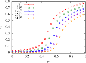
With increasing volume the transition shifts to larger values of the coupling and we conclude that in the infinite volume limit the theory is in the symmetric regime for every finite value of the coupling, as predicted by the Mermin-Wagner theorem. It is also evident that finite volume effects are more important for large coupling. In particular, the observed behaviour might mimic an additional non-trivial fixed point of the RG flow. In Fig. 4 we show the -function for the coupling in the simplest truncation using only the operator .
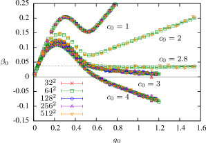
We observe that while the -function is independent of the lattice volume, it depends on the parameter of the RG transformation. For the function has an IR fixed point at vanishing coupling and stays positive even for large coupling. Tuning to larger values, the -function develops a further zero crossing at finite coupling. However, this additional zero of the -function is an artifact of the truncation. In Fig. 5 we show the ratio of correlation lengths of the original ensemble on the lattice compared to the truncated ensemble on the lattice. Truncation errors are assumed to be minimal for .
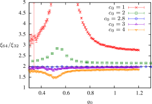
For and significant deviations are visible. We find that provides a good matching for a large range of couplings. The corresponding beta function in Fig. 4 does not show an additional zero crossing, which coincides with earlier results Shenker and Tobochnik (1980). For large the function approaches a constant value corresponding to the large result Hirsch and Shenker (1983). In order to further improve on our truncation, we add a second operator and the resulting flow diagram for fixed and different lattice sizes is shown in Fig. 6.


The flow is no longer independent of the volume and for the smallest
lattice, which is , an additional fixed point in the
(, )-plane emerges.
However, going to larger lattice volumes, this fixed point shifts away
towards larger couplings and thus we assume that in the continuum
limit no additional fixed point of the RG flow exists.
The renormalized trajectory is the single trajectory that connects the
Gaußian fixed point at the origin with the trivial fixed point
at infinite coupling. The arrows plotted in Fig. 6
point towards the IR and therefore the fixed point at the origin
is an IR fixed point while the fixed point at infinite coupling is UV
attractive. Again we find that the structure of the flow diagram
using the two-operator truncation matches the prediction from
asymptotic freedom. The known results are very well reproduced with
our method and we proceed with the O(N) models in three spacetime
dimensions.
V Fixed Points of the RG Flow in three dimensions
As in two dimensions we first investigate the O(3) model. In Fig. 7 the order parameter for the spontaneous breaking of the O(N) symmetry is shown.
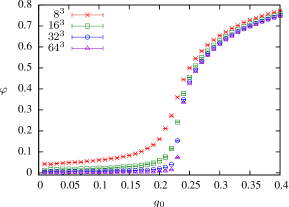
The critical coupling in the thermodynamic limit is given by Campostrini et al. (2002). On a lattice, lattice artifacts are already sufficiently small for our purpose. Therefore most RG transformations considered in the present work are based on a transformation for a fine lattice with points to a coarse lattice with points. The critical coupling on the lattice is .
V.1 One-parameter effective action
We begin with the simplest truncation possible by using
the one-parameter action .
We denote this scheme as truncation, indicating the
use of the one-parameter
action in both ensemble creation and effective action ansatz.
As in two dimensions, the function for this truncation is
almost independent of the lattice size. Using different sizes, we see
that our results from and already agree within their
statistical error bars and therefore we are confident that our simulations
on a lattice with points do not suffer from large finite size effects.
In order to determine the optimization constant in the
blockspin transformation, we again consider the correlation length of
the two-point function. A perturbative calculation Hasenfratz et al. (1984)
yields for arbitrary N and a large number of
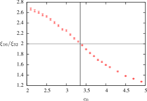
subsequent RG steps. But computing the ratio of correlation lengths (see
Figure 8), we see that there exists an optimal choice
which leads to the desired value of
. This value deviates significantly
from , indicating that the non-trivial fixed
point is indeed a non-perturbative feature of the theory.
Already with this simple setup, we find that the dimensionless function, depicted in Fig. 9, exhibits the qualitative features that were expected from other methods A.M. and Polyakov (1975); Brézin and Zinn-Justin (1976); Bardeen et al. (1976); I.Ya and Aref’eva (1979); Codello and Percacci (2009).
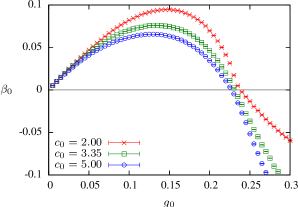
In contrast to the two dimensional case, the function
shows a non-trivial fixed point with for every
value of . This clearly points to the non-perturbative
renormalizability of the O(3) -model and is directly related to a
second-order phase transition. For
the optimal choice we obtain . Systems
with bare coupling flow to the disordered phase in the IR
which is controlled by the Gaußian fixed point at , while
systems with bare coupling flow to the completely ordered
phase described by or .
These two fixed points correspond to the expected low-temperature fixed point at
infinite coupling (absolute order) and the expected
high-temperature fixed point at
zero coupling (absolute disorder). The critical hypersurface is reduced
to a single point in this truncation and the operator
corresponds to a relevant direction of the RG flow.
Using the information provided by thermodynamical observables like e.g.
the susceptibility of the order parameter, we can determine the
critical point where the correlation length of the system
diverges at infinite volume. In general theory space, it is the
point of intersection between the critical hypersurface and the line
where except . A lattice simulation starting at in the UV
will flow along the critical line into the
non-trivial fixed point and observables measured on this ensemble reflect
the macroscopic physics at this point. Please note that need not
be identical to due to truncation errors that affect the value
for . Of course, without truncation errors the fixed
point is located at the critical surface.
We now proceed to discuss higher-order truncations which take additional
operators into account and provide a more complete picture of the flow
of the effective action.
V.2 Higher-order truncations
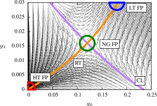
In the preceding sections we have seen that near the non-trivial fixed point the operator defines a relevant direction. In this section we include more operators in the effective action in order to find the total number of relevant directions. Figure 10 (upper panel) shows the global flow diagram for the truncation using two operators , both for ensemble generation as well as in the demon method ( truncation).


The blockspin transformation is optimized in the same way as for the action
with a single parameter. Our choice for the parameters is and
and it leads to a correlation length ratio of around in
the vicinity of the fixed point. Note that this choice for the parameters is not unique if we only tune the correlation length to the desired value. In general we have to
consider higher correlation functions as well. Below we will also discuss other choices for the parameters and its
influence on quantitative features of the flow diagram as for example the position of the fixed point or critical exponents.
Nevertheless as in the one parameter case the choice of the parameters does not change the qualitative flow diagram.
Again, we detect a high temperature fixed point (HT FP) at zero coupling in the lower left corner
as well as a low temperature fixed point (LT FP) at infinite
coupling. Also a non-trivial fixed point (NG FP) in the center
of the flow diagram is clearly visible. The values of the couplings at the fixed point,
, , can be determined from Fig. 10
(lower panel). As expected, the ‘velocity’ along a trajectory gets small in the
fixed point regime. Furthermore, we find that the position of the fixed
point in this two parameter truncation is almost independent of the
lattice volume. But, in contrast to the one-parameter truncation,
it depends strongly on the constant and to a lesser degree on the
remaining constants. A change of results in
a displacement of the fixed point along the critical line.
The flow diagram is split by a separatrix which defines the
critical line (CL) extending from the lower right to the
upper left corner. Trajectories that lie above this line will flow into
the low temperature fixed point while trajectories below this line flow
into the high temperature fixed point. This indicates a relevant
direction analogous to the simple
one-parameter truncation of the preceding section. The second direction
though is an irrelevant one and the corresponding eigenvalue of
the stability matrix is negative. The single
trajectory that is identical with the critical line
will flow into the non-trivial fixed point, either from below or above.
The critical line is the intersection of the critical hypersurface in
general theory space with the - plane that constitutes
our truncation. From the traditional lattice perspective, the critical
line corresponds
to a fine-tuned set of bare couplings , at different
UV cutoffs. Starting a simulation on the critical line results in a
measurement of the critical physics at the non-trivial fixed point and
is generically used to take the continuum limit, since the lattice spacing in units
of the correlation length becomes small as the critical point is
approached.
There exists another interesting line which connects all three fixed points
and acts as an attractor for the RG trajectories. It is called
the renormalized trajectory (RT) and singles out a unique
trajectory that defines a theory that is both IR and UV complete,
starting at the non-trivial fixed point in the UV and flowing into the
high temperature or low temperature fixed point in the IR. As expected, the
RT does not attract the trajectories in the vicinity of the high temperature
fixed point, where the fixed point behaviour dominates
111For this reason the matching method is not applicable in the vicinity of the
high temperature fixed point since it relies on the assumption that the
trajectories approach the renormalized trajectory within a few
RG steps Hirsch and Shenker (1983)..
Starting on the axis, which corresponds to the usual lattice
action of the Heisenberg ferromagnet, and integrating out all
fluctuations, one can only reach either one of the trivial fixed points
or the non-trivial fixed point. In this sense, it is
legitimate to consider them as infrared fixed points. From
universality arguments one expects that the non-Gaußian fixed point corresponds
to the well-known Wilson-Fisher fixed point of the linear sigma model.
We find that a similar structure to our results emerges in this model Bohr et al. (2001).
But the Heisenberg ferromagnet is an effective theory that is
well defined only for a finite UV cutoff, in contrast to
asymptotically safe theories that are defined on all scales.
Fundamental field theories correspond to theories on the renormalized
trajectory and the direction of the renormalization group flow shows
that the non-trivial fixed point governs the ultraviolet
physics of these theories. Thus, this non-trivial fixed point acts
as an ultraviolet fixed point of the RG flow.
For the asymptotic safety scenario to hold, the number
of relevant directions at the non-Gaußian fixed point must be
finite. Hence we proceed to determine the flow diagram for the
and truncation, which include the operators
, and
respectively. An overview over the full flow diagram for
the operators is presented in Figure 11 and
it is evident that only irrelevant directions are added to the
truncation. The global structure of the flow diagram is similar to
the truncation and shows two trivial IR fixed points
and one non-trivial UV fixed point.
Figure 12 (upper panel) shows a detailed view of
the the fixed point regime. The fixed point is located at
.
In the center panel of Figure 12 the
truncation with operators is presented.
The resulting flow diagram is again very similar and we find that even
the position of the fixed point at
matches the prior result
within the resolution of the flow diagram.
Finally Fig. 12
(lower panel) shows the results for the truncation.
Again the fixed point structure remains unchanged. In this truncation
the position of the fixed point is at .
In conclusion, we observed that the fixed point structure does not change
if we add further operators. We always find just one relevant direction
at the non-Gaußian fixed point. In addition the position of the fixed point
is stable against including the higher derivative operators and .
This clearly points to the existence of a non-Gaußian
fixed point of the RG transformation and thus we are led to believe
that the asymptotic safety scenario applies to the O(3) nonlinear sigma
model in three dimensions.
V.3 Critical exponents
Following the universality hypothesis, it is generally
assumed that the linear and nonlinear O(N) models are in the same
universality class, since they have the same range of interaction
and symmetries. This assumption is supported by several computations
based on very different approximations, cf. for
instance Zinn-Justin (1996); Ballesteros et al. (1996); Butera and Comi (1997) or the overviews
Pelissetto and Vicari (2002); Wipf (2013).
Furthermore, critical exponents are universal,
in contrast to the position of the fixed point, and this allows us to compare
our results to the functional RG studies of the nonlinear
O(N) models in Flore et al. (2013).
Here we restrict ourselves to the scaling properties of the
correlation length, described by the exponent , since it is
directly related to the relevant eigenvalue
of the stability matrix by .
Using the simple truncation, the inverse of the
thermodynamic critical exponent corresponds to the negative slope of the lattice beta
function in the vicinity of a fixed point, depicted in Fig. 9.
As expected, we find the trivial values and for the
high-temperature and low-temperature fixed points, respectively.
These values are almost independent of . For the non-trivial fixed point,
on the other hand, the value depends on the choice for , and
this is shown in Fig. 13.
For the optimal constant we read off the critical exponent for , which is to be compared with the value in Campostrini et al. (2002) obtained from a dedicated Monte Carlo simulation combined with high-temperature expansions. In Fig. 14 the critical exponent is shown as a function of .
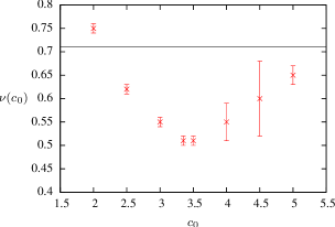
Again one sees that a careful optimization of the blockspin transformation
is important in order to extract accurate results for the critical exponents.
The next improvement is to allow 2 operators in the effective action,
denoted as truncation. The critical exponent
is determined as the negative slope of the projected -function on the
axis at the position of the fixed point for the
truncation. For the optimized we obtain
. This is already significantly closer to
the expected value compared with the simple
truncation.
We can further improve our estimate by moving on to the truncation.
Depicted in Figure 15 (upper panel) is the eigenvalue
of the matrix (18), which at a critical point becomes
the stability matrix, and
again it takes the trivial values at the high temperature or low temperature fixed
point.
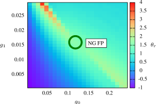
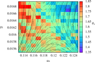
While the plot shows strong variations of the eigenvalue at
the upper left and lower right corner of the parameter space, it
becomes smooth in the vicinity of the non-trivial fixed point,
see Fig. 15 (lower panel).
From an average over the fixed point region we
obtain the value of , which already
deviates less than from the literature value. We stress
that in the present work we are mainly concerned with the flow diagram
and fixed point structure of non-linear O(N) -models such that our method
is not to be seen as a replacement of dedicated high-precision
Monte Carlo determination of critical exponents.
It is however possible to estimate these quantities in addition to the
flow diagram with a reasonable precision.
In the truncation we can also extract the critical exponent corresponding
to the irrelevant direction of the flow, see Fig. 16.
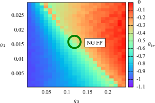
It takes the trivial value at the high temperature fixed point
and at the non-Gaußian fixed point.
In order to check for the stability of our method we calculated the critical exponent also for the RG parameters and . We obtained the value
. Within statistical errors this agrees with the value for obtained before.
For the truncation we set the RG parameter belonging to the additional operator to zero, i.e. , and .
In this truncation we obtain three critical exponents:
| (33) | ||||
The exponent of the correlation length is then . Within
statistical errors this is almost no improvement compared to the
truncation.
Our analysis of the critical exponents indicates that the high temperature fixed point has
only irrelevant directions,
i.e. all critical exponents are negative. The exponents corresponding to the operators and take the value .
The non-Gaußian UV fixed point has one positive critical exponent, while the other critical exponents are negative.
This again verifies the asymptotic safety scenario for the nonlinear sigma model in three dimensions.
Table 1 summarizes our results for the critical exponents.
| Method | ||
|---|---|---|
| trunc. () | ||
| trunc. () | ||
| trunc. () | ||
| trunc. () | ||
| trunc. () | ||
| FRG Flore et al. (2013) | ||
| MC Campostrini et al. (2002) | ||
| RG Antonenko and Sokolov (1995) | ||
| HT Butera and Comi (1997) |
For comparison we also show results obtained with Monte Carlo simulations (MC), high temperature expansion (HT), RG expansion (RG) and functional RG (FRG). With increasing truncation order our results approach the very precise values obtained with other methods, indicating that our derivative expansion converges to the correct results. For even higher truncations the computation of critical exponents becomes very time consuming and the statistical errors become larger than the deviation from the values in the literature. Furthermore the optimization of the blockspin transformation becomes increasingly difficult. Nevertheless results are good enough to show that the non-Gaußian UV fixed point indeed belongs to a well-known class of second order phase transitions.
VI The large limit
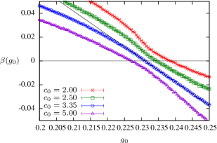
For large values of we can compare our results with those from the analytical large and RG expansions in Okabe and Oku (1978) and Antonenko and Sokolov (1995), respectively. In Fig. 17 the -function in the truncation is shown for different at the optimized value for .
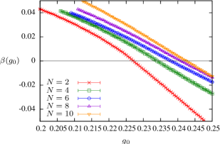
For every value of a non-trivial fixed point exists, but the slope at the fixed point changes. In order to connect to the large limit, we repeat the computation of the critical exponent in the simple truncation for up to . The results are shown in Fig. 18.
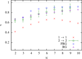
Starting from , where the estimate deviates from the comparative RG data by , we see a significant improvement for intermediate . However, going to even larger , the behaviour changes and our results significantly underestimate the correct values. It is evident that we do not reproduce the analytically known result of for .
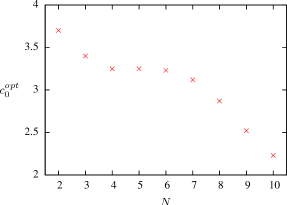
This change of behaviour is not only visible in the critical exponents but
also shows up in the value of the optimization constant .
From the perturbative analysis Hasenfratz et al. (1984), we know that for
large the RG parameter is proportional to , i.e. we
expect to become constant for large .
Indeed in Figure 19 we see a plateau for intermediate values of .
Unfortunately, for the optimization
constant decreases rapidly. We interpret this unexpected behaviour as a
breakdown of our simple one parameter truncation for large . If the
effective action does not capture the relevant physics anymore, then we
should not expect to find reliable values for the critical exponents.
Although we can tune the ratio of two-point functions to the desired
value, higher correlation functions should indicate that, within our
truncation, the IR physics changes under the RG transformation.
We might try to improve the situation by including higher order
operators. For the truncation we calculated the critical
exponents up to and actually see a
significant improvement over the truncation,
see Fig. 18. It turns out that, compared to the literature, we get the best results if we set the
RG parameter to the values obtained in the simplest truncation for and to the plateau value for .
For the second operator we choose . We checked that the ratio of the correlation length is approximately in the vicinity of
the fixed point for this set of parameters.
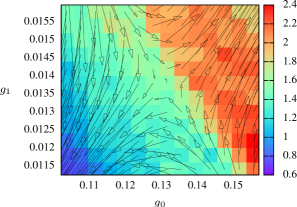
In Figure 20, we show
that for different the general structure of the flow diagram
persists. Only the non-universal location of the non-Gaußian fixed point
varies.
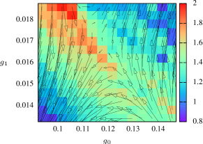
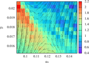
Unfortunately the fine-tuning of the RG parameter and the computation of critical exponents becomes increasingly difficult for even larger . We again observe that for our truncation breaks down and additional operators are needed to obtain reliable results for the critical exponents. Nevertheless the fixed point structure itself remains stable. Our final results are compiled in Table 2 and Figure 18.
VII Conclusions
We have discussed and applied a method that allows to compute the global flow
diagram of a model from numerical simulations. In contrast to the
MCRG matching technique, our method does not need exponentially large
lattices and works even in the vicinity of a Gaußian fixed point,
where the renormalized trajectory no longer acts as an attractor for
the RG flow. Furthermore, we have shown that systematic uncertainties
from a truncation of the effective action can be mitigated efficiently
by an optimization of the RG transformation.
The nonlinear sigma model is asymptotically free in two dimensions and
we have reproduced the expected structure of the flow diagram,
showing two trivial fixed
points corresponding to the behaviour at very low and
very high temperature, already using the simplest
possible truncation that only includes a nearest-neighbor interaction.
Using a two-operator truncation, we have clarified the role of the
finite volume behaviour on the flow diagram and argued
that an additional non-trivial fixed point is a lattice
artifact.
It has long been known that the three-dimensional O(3) -model shows a
second-order phase transition that separates a phase of broken O(N) symmetry and a symmetric phase. We have shown that this phase transition
corresponds to an ultraviolet fixed point with one relevant direction
by using a truncation that includes all (allowed by symmetry) operators
up to fourth order in the momentum.
It is possible to define a theory along the renormalized trajectory
that is IR- and UV-complete. We conclude that the asymptotic safety
scenario is fulfilled and the model is renormalizable in a
non-perturbative setting.
While the general structure of the flow diagram does not depend on the
specific RG scheme the critical exponents vary since the systematic
error depends on the specific optimization constant. We find that our
method is able to predict the critical exponents within a reasonable
accuracy but can not compete to designated high precision
MC-techniques that are free of truncation errors
Campostrini et al. (2002). We find that our estimates for the critical
exponents improve for larger truncations but fail to reproduce the
exact limit.
Using functional renormalization group techniques, the
full flow diagram for the present model was obtained already in an earlier
publication Flore et al. (2013). We find that the qualitative structure of
the flow diagrams are the same. However, the MCRG method
is more stable than the FRG method and leads to more robust
results for different truncations. In particular, we do not find a sudden
disappearance of the non-trivial fixed point for a certain truncation
including the operator (28).
Furthermore, we stress that lattice techniques provide
the opportunity to obtain additional information beyond the chosen
truncation by a direct measurement of the Green’s functions.
We have used this knowledge to determine the
optimal constants in the improved RG transformation. In addition
we compared the location of the critical point, determined by the
susceptibility of the order parameter, to the location of the fixed
point, determined by the zero crossing of the beta function
and hence amendable to truncation errors. We find that these points do
not coincide in general. For the simplest truncation we observe a small
deviation even for the optimal value of the RG constant.
For higher truncations, the fixed point location matches the critical
surface within statistical errors. Another interesting observation is
that the function in the lowest truncation for two and three
dimensions does not depend on the lattice size.
Our method can be generalized to other systems, especially including
fermionic degrees of freedom, and thus allows to determine the more
complex flow diagrams of e.g. the Thirring model Gies and Janssen (2010).
The method might also be used to study lattice quantum gravity
Ambjorn et al. (2001, 2013) where it is difficult to define
observables that capture the infrared physics of the theory.
In contrast to the matching technique, the method used in the present
work does not rely on the computation of correlation functions but only
on an appropriate RG transformation that acts directly on the spacetime
triangulations used.
Acknowledgements.
This work was supported by the DFG-Research Training Group ”Quantum- and Gravitational Fields” GRK 1523 and DFG grant Wi777/11 and by the Helmholtz International Center for FAIR within the LOEWE initiative of the State of Hesse. We thank Raphael Flore for his active collaboration and Jens Braun, Axel Maas, Roberto Percacci, Martin Reuter, Omar Zanusso and Luca Zambelli for interesting discussions or useful comments. Simulations were performed on the Omega HPC cluster at the University of Jena and the LOEWE-CSC at the University of Frankfurt.Appendix A Two Alternative Formulations of a Fourth-Order Derivative Expansion
In this article we study the full fourth order derivative expansion of the theory, formulated in terms of explicitly constrained variables with . In order to compare the results with previous studies of the same system by means of the Functional Renormalization Group (FRG) Flore et al. (2013), one has to know the relation between both parametrizations of the action functional. The FRG computations in Flore et al. (2013) were performed for the covariant formulation
| (34) | ||||
in terms of unconstrained fields , where and is the Christoffel symbol corresponding to the metric . In order to determine the relation between (34) and (19), one can choose stereographic coordinates,
| (35) |
for an unconstrained parametrization of (34) and apply an inverse stereographic projection,
| (36) |
such that
| (37) | ||||
A comparison with (19) yields
| (38) |
Appendix B The LHMC algorithm
In the case of nonlinear sigma models with only the standard interaction term , cluster algorithms have proven to be the most efficient way to update the scalar field in Monte-Carlo simulations. In its original version, the cluster algorithm assumes that only nearest neighbor interactions are present and hence is not directly applicable in the presence of higher derivative operators. Thus we employ a local version of the hybrid Monte-Carlo algorithm (LHCM) where single site variables are evolved in an HMC algorithm. This ansatz relies on local interactions and is applicable theories without dynamical fermions. The formulation is given entirely in terms of SO(N) -Lie-group and Lie-algebra elements, see also Wellegehausen et al. (2011). To update the normalized scalar field we set
| (39) |
and constant . The change of variables converts the induced measure on into the Haar measure of SO(N) . Without interaction the rotation matrices will evolve freely on the group manifold SO(N) . The free evolution on a semisimple group is the Riemannian geodesic motion with respect to the Cartan-Killing metric
| (40) |
The LHMC dynamics may be naturally derived from a Lagrangian of the form
| (41) |
where ‘dot’ denotes the derivative with respect to the fictitious time parameter . The Lie-algebra valued pseudo-momenta conjugated to the site variable are given by
| (42) |
The Legendre transform yields the following pseudo-Hamiltonian
| (43) |
Note that for SO(N) the momenta are antisymmetric such that the kinetic term is positive. The equations of motion for the momenta are obtained by varying the Hamiltonian,
| (44) |
In the simplest case of only nearest neighbor interactions the force is given by
| (45) |
The variational principle implies that the projection of the terms between curly brackets onto the Lie-algebra vanishes,
| (46) |
There is a freedom of choice of and we determine it by a projection on a trace-orthonormal basis of . Then the LHMC equations read
| (47) |
To solve these equations of motion numerically, we employ a time reversible leap frog integrator which uses the integration scheme
| (48) | ||||
References
- Wilson (1975) K. G. Wilson, Rev. Mod. Phys. 47, 773 (1975).
- Wetterich (1993) C. Wetterich, Physics Letters B 301, 90 (1993).
- Hawking and Israel (1979) S. Hawking and W. Israel, eds., General Relativity, an Einstein Centenary Survey (Cambridge University Press, Cambridge, 1979).
- Niedermaier and Reuter (2006) M. Niedermaier and M. Reuter, Living Reviews in Relativity 9 (2006).
- Reuter and Saueressig (2002) M. Reuter and F. Saueressig, Phys. Rev. D 65, 065016 (2002).
- Benedetti et al. (2009) D. Benedetti, P. F. Machado, and F. Saueressig, Mod.Phys.Lett. A24, 2233 (2009), arXiv:0901.2984 [hep-th] .
- Litim (2011) D. F. Litim, Phil.Trans.Roy.Soc.Lond. A369, 2759 (2011), arXiv:1102.4624 [hep-th] .
- Lüscher et al. (1991) M. Lüscher, P. Weisz, and U. Wolff, Nucl. Phys. B 359, 221 (1991).
- Tröster (2011) A. Tröster, Computer Physics Communications 182, 1837 (2011).
- Hasenfratz et al. (1984) A. Hasenfratz, P. Hasenfratz, U. Heller, and F. Karsch, Physics Letters B 140, 76 (1984).
- Hasenfratz and Margaritis (1984) A. Hasenfratz and A. Margaritis, Phys.Lett. B148, 129 (1984).
- Ma (1976) S.-K. Ma, Phys. Rev. Lett. 37, 461 (1976).
- Lang (1986) C. Lang, Nucl.Phys. B265, 630 (1986).
- Catterall et al. (2012) S. Catterall, L. Del Debbio, J. Giedt, and L. Keegan, Phys. Rev. D85, 094501 (2012), arXiv:1108.3794 [hep-ph] .
- Bock and Kuti (1996) W. Bock and J. Kuti, Physics Letters B 367, 242 (1996).
- Shenker and Tobochnik (1980) S. H. Shenker and J. Tobochnik, Phys. Rev. B 22, 4462 (1980).
- Creutz et al. (1984) M. Creutz, A. Gocksch, M. Ogilvie, and M. Okawa, Phys. Rev. Lett. 53, 875 (1984).
- Hasenbusch et al. (1995) M. Hasenbusch, K. Pinn, and C. Wieczerkowski, Nucl. Phys.Proc.Suppl. 42, 808 (1995), arXiv:hep-lat/9411043 [hep-lat] .
- Wozar et al. (2008) C. Wozar, T. Kastner, B. H. Wellegehausen, A. Wipf, and T. Heinzl, PoS LATTICE2008, 257 (2008), arXiv:0808.4046 [hep-lat] .
- Campostrini et al. (2006) M. Campostrini, M. Hasenbusch, A. Pelissetto, and E. Vicari, Phys. Rev. B74, 144506 (2006), arXiv:cond-mat/0605083 [cond-mat] .
- Gasser and Leutwyler (1984) J. Gasser and H. Leutwyler, Annals of Physics 158, 142 (1984).
- A.M. and Polyakov (1975) A.M. and Polyakov, Physics Letters B 59, 79 (1975).
- Brézin and Zinn-Justin (1976) E. Brézin and J. Zinn-Justin, Phys. Rev. Lett. 36, 691 (1976).
- Bardeen et al. (1976) W. A. Bardeen, B. W. Lee, and R. E. Shrock, Phys. Rev. D 14, 985 (1976).
- I.Ya and Aref’eva (1979) I.Ya and Aref’eva, Annals of Physics 117, 393 (1979).
- Codello and Percacci (2009) A. Codello and R. Percacci, Physics Letters B 672, 280 (2009).
- Flore et al. (2013) R. Flore, A. Wipf, and O. Zanusso, Phys. Rev. D87, 065019 (2013), arXiv:1207.4499 [hep-th] .
- Koerner et al. (2013) D. Koerner, B. H. Wellegehausen, and A. Wipf, (2013), arXiv:1310.8202 [hep-lat] .
- Butera and Comi (1997) P. Butera and M. Comi, Phys. Rev. B 56, 8212 (1997).
- Campostrini et al. (2002) M. Campostrini, M. Hasenbusch, A. Pelissetto, P. Rossi, and E. Vicari, Phys. Rev. B65, 144520 (2002), arXiv:cond-mat/0110336 [cond-mat] .
- Antonenko and Sokolov (1995) S. Antonenko and A. Sokolov, Phys. Rev. E51, 1894 (1995), arXiv:hep-th/9803264 [hep-th] .
- Chen et al. (1993) K. Chen, A. M. Ferrenberg, and D. Landau, Phys. Rev. B48, 3249 (1993).
- Kadanoff (1966) L. P. Kadanoff, Physics 2 , 263 (1966).
- Hirsch and Shenker (1983) J. E. Hirsch and S. H. Shenker, Phys. Rev. B 27, 1736 (1983).
- Bohr et al. (2001) O. Bohr, B. Schaefer, and J. Wambach, Int.J.Mod.Phys. A16, 3823 (2001), arXiv:hep-ph/0007098 [hep-ph] .
- Zinn-Justin (1996) J. Zinn-Justin, Quantum Field Theory and Critical Phenomena, 3rd ed. (Clarendon Press, 1996).
- Ballesteros et al. (1996) H. Ballesteros, L. Fernández, V. Martín-Mayor, and A. M. Sudupe, Physics Letters B 387, 125 (1996).
- Pelissetto and Vicari (2002) A. Pelissetto and E. Vicari, Physics Reports 368, 549 (2002).
- Wipf (2013) A. Wipf, Lect. Notes Phys. 864 (2013), 10.1007/978-3-642-33105-3.
- Okabe and Oku (1978) Y. Okabe and M. Oku, Prog.Theor.Phys. 60, 1287 (1978).
- Gies and Janssen (2010) H. Gies and L. Janssen, Phys. Rev. D82, 085018 (2010), arXiv:1006.3747 [hep-th] .
- Ambjorn et al. (2001) J. Ambjorn, J. Jurkiewicz, and R. Loll, Nucl. Phys. B610, 347 (2001), arXiv:hep-th/0105267 [hep-th] .
- Ambjorn et al. (2013) J. Ambjorn, A. Goerlich, J. Jurkiewicz, and R. Loll, (2013), arXiv:1302.2173 [hep-th] .
- Wellegehausen et al. (2011) B. H. Wellegehausen, A. Wipf, and C. Wozar, Phys.Rev. D83, 114502 (2011), arXiv:1102.1900 [hep-lat] .