Toward the Standard Population Synthesis Model of the X-Ray Background: Evolution of X-Ray Luminosity and Absorption Functions of Active Galactic Nuclei Including Compton-Thick Populations

Abstract

We present the most up-to-date X-ray luminosity function (XLF) and absorption function of Active Galactic Nuclei (AGNs) over the redshift range from 0 to 5, utilizing the largest, highly complete sample ever available obtained from surveys performed with Swift/BAT, MAXI, ASCA, XMM-Newton, Chandra, and ROSAT. The combined sample, including that of the Subaru/XMM-Newton Deep Survey, consists of 4039 detections in the soft (0.5–2 keV) and/or hard ($>2$ keV) band. We utilize a maximum likelihood method to reproduce the count-rate versus redshift distribution for each survey, by taking into account the evolution of the absorbed fraction, the contribution from Compton-thick (CTK) AGNs, and broad band spectra of AGNs including reflection components from tori based on the luminosity and redshift dependent unified scheme. We find that the shape of the XLF at $z\sim 1-3$ is significantly different from that in the local universe, for which the luminosity dependent density evolution model gives much better description than the luminosity and density evolution model. These results establish the standard population synthesis model of the X-Ray Background (XRB), which well reproduces the source counts, the observed fractions of CTK AGNs, and the spectrum of the hard XRB. The number ratio of CTK AGNs to the absorbed Compton-thin (CTN) AGNs is constrained to be $\approx$0.5–1.6 to produce the 20–50 keV XRB intensity within present uncertainties, by assuming that they follow the same evolution as CTN AGNs. The growth history of supermassive black holes is discussed based on the new AGN bolometric luminosity function.

1. Introduction

Understanding the cosmological evolution of supermassive black hole (SMBHs) is a key issue in modern astrophysics. The good correlation of the mass of a SMBH in a galactic center with that of the bulge in the present-day universe (e.g., Magorrian et al., 1998; Ferrarese & Merritt, 2000; Gebhardt et al., 2000; Marconi & Hunt, 2003; Häring & Rix, 2004; Hopkins et al., 2007; Kormendy & Bender, 2009; Gültekin et al., 2009) indicates that SMBHs and galaxies co-evolved in the past. This idea is also supported by the similarity of the global history between star formation and SMBH growth (Marconi et al., 2004). The so-called down-sizing or anti-hierarchical evolution, the trend that more massive systems formed in earlier cosmic time, has been revealed for both SMBHs (Ueda et al. 2003, U03; Hasinger et al. 2005, H05) and galaxies (e.g., Cowie et al., 1996; Kodama et al., 2004; Fontanot et al., 2009).

Active galactic nuclei (AGNs) are the phenomena where SMBHs gain their masses from accreting gas by converting a part of their gravitational energies into radiation. It is known that the majority of AGNs are obscured by gas and dust surrounding the SMBHs, being classified as “type-2” AGNs. To elucidate the growth history of SMBHs, a complete survey of AGNs including heavily obscured populations throughout the history of the universe is necessary. X-ray observations, in particular those at high energies above a few keV, provide one of the most powerful approach for AGN detection thanks to the strong penetrating power against absorption and little contamination from star lights in the host galaxies. Furthermore, the deepest X-ray surveys currently available achieve the highest sensitivity even for unobscured (“type-1”) AGNs among those at any wavelengths (see Brandt & Hasinger, 2005, and references therein). The surface number density of the faintest X-ray AGNs reaches $\sim 10^{4}$ deg^-2 (Xue et al., 2011).

The integration of emission from all accreting SMBHs in the universe is observed as the X-ray background (XRB). To quantitatively solve the XRB origin is equivalent to revealing the cosmological evolution of AGNs that constitute the XRB. The XRB spans over a wide energy range from $\sim$0.1 keV to $\sim$100 keV and then is smoothly connected to the gamma-ray background at higher energies. Its spectrum has a peak energy density around $\sim$20 keV. At energies below $\sim$8 keV, now almost all of the XRB is resolved into discrete sources, mainly AGNs. Enormous efforts have been made to identify AGNs detected in X-ray surveys on the basis of multiwavelength observations, and the redshifts (and hence luminosities) of a large fraction of these sources are now estimated. These results make it possible to determine the spatial number density of AGNs that constitute the XRB below $\sim$8 keV and its evolution. By contrast, in the hard X-ray band above $\sim$10 keV, a significant fraction of the XRB is still left unresolved. Therefore, at present, the whole origin of the XRB over the wide range cannot be directly revealed by resolving individual sources.

It is very important to construct a “population synthesis model” of the XRB where the evolutions of all X-ray emitting AGNs with various types are formulated (for previous works, see e.g. Comastri et al., 1995; Gilli et al., 1999; Ueda et al., 2003; Ballantyne et al., 2006; Gilli et al., 2007; Treister et al., 2009). The model, in principle, must explain all the observational constraints including source number counts, redshift and luminosity distribution, the shape of the XRB. Once established, it gives the basis to understand the accretion history of the universe traced by X-rays, which is subject to least biases.

Two major elements in the population synthesis models are the X-ray luminosity function (XLF) and absorption function (or $N_{\rm H}$ function, Ueda et al. 2003) of AGNs. The XLF represents the number density of AGN per comoving space as a function of luminosity and redshift, one of the most important statistical quantity that can be determined from unbiased surveys. Previously many studies have been made on the cosmological evolutions of the XLF of AGNs in the soft band below 2 keV (e.g., Maccacaro et al., 1991; Boyle et al., 1993; Jones et al., 1997; Page et al., 1997; Miyaji et al., 2000; Hasinger et al., 2005) and the hard band above 2 keV (e.g., Ueda et al., 2003; La Franca et al., 2005; Barger et al., 2005; Silverman et al., 2008; Ebrero et al., 2009; Yencho et al., 2009; Aird et al., 2010). By using hard X-ray selected samples that contain both type-1 (unabsorbed) and type-2 (absorbed) AGNs, the absorption functions have been also investigated (Ueda et al., 2003; La Franca et al., 2005; Ballantyne et al., 2006; Treister & Urry, 2006; Hasinger, 2008). Besides the well established anti-correlation of absorption fraction with luminosity (e.g., Ueda et al., 2003; Steffen et al., 2003; Simpson, 2005), several works have reported that the fraction of absorbed AGNs increased toward higher redshift from $z=0$ to $z>1$ (La Franca et al., 2005; Ballantyne et al., 2006; Treister & Urry, 2006; Hasinger, 2008). More recent studies of high redshift AGNs at $z>2$ in deep fields (Hiroi et al. 2012; Iwasawa et al. 2012) reveal larger absorption fractions of high luminosity AGNs compared with the local universe. This redshift evolution is not included in the population synthesis model by Gilli et al. (2007), one of the most widely referred model available at present.

There still remain uncertainties on the evolution of AGNs, however. The first issue is the shape of the XLF and its cosmological evolution. On the basis of hard X-ray surveys, Ueda et al. (2003), Silverman et al. (2008), Ebrero et al. (2009), and Yencho et al. (2009) find that the XLF of AGN is best described with the luminosity dependent density evolution (LDDE) model. Later, Aird et al. (2010) propose that the luminosity and density evolution (LADE) where the shape of the XLF is constant over the whole redshift range unlike the case of LDDE also gives a similarly good fit to their data. While the down-sizing behavior is commonly seen in both models, quite different number of AGNs are predicted particularly at high redshifts of $z\geq 3$. The second one is the number density (or fraction) of heavily obscured AGNs with $N_{\rm H}$ $>10^{24}$ cm^-2, so-called “Compton-thick” AGNs (CTK AGNs). Even hard X-ray surveys above 10 keV are subject to bias against detecting heavily CTK AGNs, because the transmitted emission is significantly suppressed due to repeated Compton scattering (see e.g., Wilman & Fabian, 1999; Ikeda et al., 2009). It is not easy to identify individual CTK AGNs with limited photon statistics in deep survey data, and to estimate their intrinsic number density by correcting for such biases.

In this work, we present our latest results of AGN XLF over the redshift range from 0 to 5, by utilizing one of the largest combined sample ever available, obtained from surveys of various depth, width, and energy bands performed with Swift/BAT, the Monitor of All-sky X-ray Image (MAXI, Matsuoka et al. 2009), ASCA, XMM-Newton, Chandra, and ROSAT. The sample consists of 4039 detections in the soft (0.5-2 keV) and/or hard ($>2$ keV) bands. We utilize a maximum likelihood (ML) method to reproduce the count-rate versus redshift distribution for each survey, by taking into account the selection biases. In the analysis, the contribution of CTK AGNs is considered, which is found to be more important in harder bands and at fainter fluxes. This enables us to determine the intrinsic XLF and the absorption function of type-1 plus type-2 AGNs with an unprecedented accuracy, thus establishing a standard population synthesis model of the XRB that is consistent with most of observational constraints currently available.

The organization of the paper is as follows. Section 2 explains the sample used in our analysis. In Section 3 the absorption properties of AGNs are discussed and the absorption function is formulated. Section 4 introduces the “template model” of broad band X-ray spectra of AGNs adopted in this work. The distribution of photon index is examined by using the Swift/BAT sample in Section 5. Section 6 describes the details of main analysis using the whole sample. The best-fit results of the XLF are presented there. The predictions from the population synthesis model are given in Section 7. We also discuss the constraints on the CTK AGN fraction and degeneracy with other parameters. Section 8 represents an determination of the bolometric luminosity function of AGNs based on our new XLF, and the growth history of SMBHs. The conclusions of our work are summarized in Section 9. The cosmological parameters of ($H_{0}$, $\Omega_{\rm m}$, $\Omega_{\lambda}$) = (70$h_{70}$ km s^-1 Mpc^-1, 0.3, 0.7) are adopted throughout the paper. The “log” symbol represents the base-10 logarithm, while “ln” the natural logarithm.

2. Sample

In order to investigate the XLF and absorption function of AGNs covering a wide range of luminosity and redshift, it is vital to construct a sample combined from various surveys with different flux limits and area. Also, high degrees of identification completeness in terms of spectroscopic and/or photometric redshift determination are required to minimize systematic uncertainties caused by sample incompleteness. Basically, X-ray surveys at higher energies are more suitable to detect obscured AGNs with less biases. Nevertheless, those in the soft band ($\approx$0.5–2 keV) are also quite useful as long as such biases are properly corrected. Generally, fainter flux limits are achieved in softer energy band thanks to the larger collecting area of X-ray telescopes. In particular, for high redshift AGNs, the reduction of observed fluxes due to photo-electric absorptions becomes less important thanks to the K-correction effect. Indeed, the soft X-ray surveys are often utilized to search for high redshift AGNs even including type-2 objects (e.g., Miyaji et al., 2000; Silverman et al., 2008).

In our study, we collect the results from surveys performed with Swift/BAT, MAXI, ASCA, XMM-Newton, Chandra, and ROSAT, by utilizing the heritage of X-ray astronomy accumulated up to present. Only those with high identification completeness ($\;\buildrel>\over{\sim}\;$90%) are included. Our sample is composed of those from the Swift/BAT 9-month survey (BAT9, Tueller et al. 2008), MAXI 7-month survey (MAXI7, Hiroi et al. 2011; Ueda et al. 2011), ASCA Medium Sensitivity Survey (AMSS, Ueda et al. 2001; Akiyama et al. 2003) and Large Sky Survey (ALSS, Ueda et al. 1999; Akiyama et al. 2000), Subaru/XMM-Newton Deep Survey (SXDS, Ueda et al. 2008; Akiyama et al. 2013), XMM-Newton survey of the Lockman Hole (LH/XMM, Hasinger et al. 2001; Brunner et al. 2008), HELLAS2XMM survey (H2X, Fiore et al. 2003), Hard Bright Serendipitous Sample in the XMM-Newton Bright Survey (HBSS, Della Ceca et al. 2004, 2008), Chandra Large Area Synoptic X-ray Survey (CLASXS, Yang et al. 2004; Steffen et al. 2004; Trouille et al. 2008), Chandra Lockman Area North Survey (CLANS, Trouille et al. 2008, 2009), Chandra Deep Survey North (CDFN, Alexander et al. 2003; Barger et al. 2003; Trouille et al. 2008) and South (CDFS, Xue et al. 2011), and various ROSAT surveys (see Miyaji et al. 2000 and H05 and references therein).

This paper presents the first work that makes use of the large X-ray sample in the SXDS (Furusawa et al., 2008; Ueda et al., 2008), one of the wide and deep multiwavelength survey projects with a comparable survey area and depth as the Cosmic Evolution Survey (COSMOS; Scoville et al. 2007), in order to constrain the XLF of AGNs with the best statistical accuracy. Also, new hard X-ray all-sky surveys with Swift/BAT and MAXI are utilized instead of HEAO1 AGN samples that were usually employed in previous studies. The other soft-band and hard-band samples adopted here are also analyzed in H05 and Hasinger (2008), respectively, although in some cases different selection criteria are applied in our analysis to increase the completeness (see below). The major difference in the soft-band sample from that used by H05 is that we include both type-1 and type-2 AGNs because we aim to investigate the evolution of the whole AGN population. We do not use the sample from the Serendipitous Extragalactic X-ray Source Identification (SEXSI) program (Eckart et al., 2006) adopted by Hasinger (2008), whose redshift identification completeness is slightly worse ($\sim$84%) than our threshold. The sample of the XMM-Newton Medium-sensitivity Survey (XMS, Barcons et al. 2007) used in Hasinger (2008) are discarded because it partially overlaps with the SXDS sample. The detailed description of each survey is given below.

2.1. Swift/BAT

We utilize the Swift/BAT 9-month catalog (Tueller et al., 2008), which originally contains 137 non-blazar AGNs with a flux limit of $2\times 10^{-11}$ erg cm^-2 s^-1 in the 14–195 keV band with the signal-to-noise ratio (SNR) $>4.0$. The Swift/BAT survey, performed at energies above 10 keV, provides us with the least biased AGN sample in the local universe against obscuration except for heavily CTK sources absorbed with $N_{\rm H}$ $\gg 10^{24}$ cm^-2 along with those of INTEGRAL (e.g., Beckmann et al., 2009). The X-ray spectra below 10 keV of all the AGNs in the sample have been obtained from extensive follow-up observations by other missions such as Swift/XRT, XMM-Newton, and Suzaku (e.g., Winter et al., 2009a; Eguchi et al., 2009; Winter et al., 2009b). Thus, we can discuss their statistical properties without incompleteness problems. Here we refer to the absorption column densities summarized in Table 1 of Ichikawa et al. (2012), where new results obtained from broad-band X-ray spectra of Suzaku are included. To define a statistical sample that is consistent with the survey area curve given in Figure 1 of Tueller et al. (2008), we further impose criteria that (1) the Galactic latitude is larger than 15 degrees ($|b|>15^{\circ}$) and (2) SNR $>4.8$. We regard the pair of the interacting galaxies NGC 6921 and MCG +04-48-002 unresolved with Swift/BAT as one source, adopting the spectral information below 10 keV of the latter. The sample consists of 87 non-blazar AGNs with identification completeness of 100%.

2.2. MAXI

We include the local AGN sample from the MAXI extragalactic survey performed in the 4–10 keV band (Ueda et al., 2011) in our analysis. While the sample significantly overlaps with the Swift/BAT 9 month sample, it is useful to directly constrain the XLF in the 2–10 keV band. The sample is collected from the first MAXI/GSC catalog at high Galactic latitudes ($|b|>10^{\circ}$) with a flux limit is $1.5\times 10^{-11}$ erg cm^-2 s^-1 (4–10 keV) based on the first 7 month data (Hiroi et al., 2011). It consists of 37 non-blazar AGNs by excluding Cen A and ESO 509–066, and is used by Ueda et al. (2011) to calculate the XLF and absorption function of AGNs in the local universe. A merit is its high completeness of identification (99.3%), and similarly to the Swift/BAT 9 month catalog, the information of the X-ray spectra below 10 keV are available for all the objects as summarized in Table 1 of Ueda et al. (2011). Unlike in U03, we do not use the local AGN samples by the HEAO1 mission (Piccinotti et al., 1982), considering the lower completeness than in the MAXI sample and systematic uncertainties of the measured fluxes close to the sensitivity limit that must be corrected for (see Shinozaki et al., 2006). Note that only 17 objects out of the total MAXI/GSC AGNs are listed in the Piccinotti et al. (1982) sample, suggesting significant long term variabilities of nearby AGNs over 30 years.

2.3. ASCA

ASCA, the fourth Japanese X-ray astronomical satellite, performed first imaging surveys in the energy band above 2 keV and provided statistical X-ray samples at $>100$ times deeper levels than that of HEAO1 A2 survey. These are still very useful to bridge the flux range between all-sky surveys and deep surveys with Chandra and XMM-Newton. In our paper we utilize the two major samples, the ASCA Large Sky Survey (ALSS) and ASCA Medium Sensitivity Survey (AMSS), both are firstly utilized by U03 to calculate the hard XLF. The ALSS covers a continuous area of 5.5 deg² near the North Galactic Pole and a flux limit of $\approx 1\times 10^{-13}$ erg cm^-2 s^-1 (2–10 keV) is achieved (Ueda et al., 1998, 1999). Thirty AGNs detected with the SIS instrument are optically identified by Akiyama et al. (2000) with 100% completeness by ignoring the one unidentified source in Akiyama et al. (2000) as fake detection (see Section 2.2.2 of U03). The AMSS is based on a serendipitous X-ray survey with the GIS instrument, whose catalogs are published in Ueda et al. (2001) and Ueda et al. (2005). We use the “AMSSn” (Akiyama et al., 2003) and “AMSSs” samples for which systematic identification programs were carried out in the northern (DEC$>20^{\circ}$) and southern sky (DEC$<-20^{\circ}$), respectively. The AMSSn and AMSSs samples contains 74 and 20 optically-identified non-blazar AGNs, respectively, with a detection significance larger than 5.5 $\sigma$ at the flux range between $5\times 10^{-12}$ erg cm^-2 s^-1 and $3\times 10^{-13}$ in the 2–10 keV band. Three X-ray sources are left unidentified, and thus the completeness is 97%. The total survey area covered by the AMSSn and AMSSs is 90.8 deg². We utilize the hardness ratio between the 2–10 (or 2–7) keV and 0.7–2 keV bands to estimate the absorption or photon index of each source in the ALSS and AMSS, while results from follow-up observations with ASCA or XMM-Newton are available for six and two sources in the ALSS and AMSS, respectively (see Section 2.2 of U03).

2.4. XMM-Newton

2.4.1 SXDS

The Subaru/XMM-Newton Deep Survey (SXDS) is one of the largest multi-wavelength surveys covering from radio to X-rays with an unprecedented combination of depth and sky area. The SXDS field is a contiguous region of $>$1 deg² centered at R.A. = 02^h18^m and Dec. = $-05^{d}00^{m}$ (J2000). The large survey area makes it possible to establish the statistical properties of extragalactic populations without being affected by cosmic variance, and is also very useful to construct a sample of sources with small surface densities, like high-luminosity AGNs (i.e., QSOs) at high redshifts. The optical photometric catalogs in the $B$, $V$, $R$, $i^{\prime}$, and $z^{\prime}$ bands obtained with Subaru/Suprime-Cam are presented in Furusawa et al. (2008), achieving the $3\sigma$ sensitivities of $B$=28.4, $V$=27.8, $R_{c}$=27.7, $i^{\prime}$=27.7, and $z^{\prime}$=26.6 (for the 2 arcsec aperture in the AB magnitudes), respectively. The deep imaging data are particularly important to reliably identify high-redshift AGNs by photometric redshifts.

The X-ray catalog of the SXDS (Ueda et al., 2008) is based on the EPIC data in the 0.3–10 keV band obtained from seven pointings performed with XMM-Newton, which covers a total of 1.14 deg². It contains 866, 1114, 645, and 136 sources with sensitivity limits of $6\times 10^{-16}$, $8\times 10^{-16}$, $3\times 10^{-15}$, and $5\times 10^{-15}$ erg cm^-2 s^-1 in the 0.5–2, 0.5–4.5, 2–10, and 4.5–10 keV bands, respectively, with a detection likelihood $\geq$ 7. The deep optical images were taken by five pointing with Suprime-Cam with a slightly different shape from that of the combined XMM-Newton image. By limiting to the area of 1.02 deg² where these optical imaging data are available, we define two independent parent samples consisting of 584 and 781 sources detected in the 2–10 keV and 0.5–2 keV bands, respectively.

The results from multiwavelength identification of the X-ray sources in the SXDS is presented in Akiyama et al. (2013). Out of the 584 (2–10 keV) and 781 (0.5–2 keV) X-ray source samples, 576 and 733 objects are left as AGN candidates, respectively, after excluding Galactic stars, stellar objects close to bright galaxies, and clusters of galaxies. Among them, 397 and 514 targets have spectroscopic redshift based on near-infrared and/optical data. For the rest, Akiyama et al. (2013) determine the photometric redshifts except for seven (2–10 keV) and eight (0.5–2 keV) objects for which the fluxes in less than 4 bands are available. The redshifts are estimated on the basis of HyperZ photometric redshift code with the Spectral Energy Distribution (SED) templates of galaxies and QSOs. In addition, constraints from the morphology and absolute magnitude limits for the galaxy and QSO templates are applied (see (Hiroi et al., 2012) and (Akiyama et al., 2013) for details). The accuracy of the photometric redshifts is found to be $\Delta z/(1+z_{\rm spec}=0.06$ as a median value. Finally, 569 and 725 AGNs detected in the 2–10 keV and 0.5–2 keV bands have either spectroscopic or photometric redshifts, among which 412 are common sources. The identification completeness is rather high, 99% both for the 2–10 keV and 0.5–2 keV samples. The hardness ratio between the 2–10 keV and 0.5–2 keV is used to estimate the absorption or photon index of each source.

2.4.2 Lockman Hole

We use both the hard-band (2–4.5 keV) and soft-band (0.5–2 keV) selected samples from the XMM-Newton deep survey of the Lockman Hole (Hasinger et al., 2001; Brunner et al., 2008). They are essentially the same as those used in the analysis by Hasinger (2008) and H05, respectively, except for small differences that (1) type-2 AGNs detected in the soft-band are also included in our analysis, unlike the case of H05 who only used type-1 AGNs, and that (2) some unpublished photometric redshifts for a few hard-band selected sources mentioned in Section 2.8 of Hasinger (2008) are not utilized and instead they are treated as unidentified objects in our analysis. The effects by the latter difference are negligible. Before the AO-2 phase 17 observations of this field were performed with XMM-Newton. The X-ray source catalog is provided by Brunner et al. (2008) from 637 ks (hard band) and the 770 ks (soft band) datasets. To maximize the completeness of redshift identification, sub-samples are defined from two off-axis intervals with different flux limits as detailed in Hasinger (2008) and H05. The survey area after this selection becomes 0.183 deg² and 0.126 deg² with the fainter flux limits of $6.1\times 10^{-15}$ erg cm^-2 s^-1 (2–10 keV) and $1.3\times 10^{-15}$ erg cm^-2 s^-1 (0.5–2 keV) for the hard- and soft-band samples, respectively. The soft (hard) band sample consists of 57 (58) AGNs having either spectroscopic or photometric redshifts (Fotopoulou et al., 2012) with identification completeness of 91% (88%). We refer to Mateos et al. (2005) for the results of X-ray spectral analysis, with some updates for sources whose redshifts are revised after the publication of Mateos et al. (2005) (Streblyanska 2006, private comm. ).

2.4.3 HELLAS2XMM

The HELLAS2XMM (Baldi et al., 2002) is a serendipitous survey performed with XMM-Newton in the 2–10 keV band. We basically refer to the original sample complied by Fiore et al. (2003) selected from five XMM-Newton fields, covering a total area of 0.9 degree². Among the 122 hard X-ray selected sources, Fiore et al. (2003) present the spectroscopic redshifts for 97 AGNs. Additional information on the redshifts of the unidentified sources in the original catalog of Fiore et al. (2003) is reported in Mignoli et al. (2004) and Maiolino et al. (2006). To ensure a high completeness, we apply a flux limit of $1.5\times 10^{-14}$ erg cm^-2 s^-1 (2–10 keV) band, which leaves 95 sources after excluding one Galactic star and one extended object. Among them, 87 AGNs have redshifts and 8 objects are left unidentified. The completeness is thus 92%. The results of X-ray spectral analysis are presented in Perola et al. (2004). Unlike in Hasinger (2008), we do not include the new catalog of HELLAS2XMM by Cocchia et al. (2007) in our analysis, considering the lower rate of redshift identification (59 out of 110 sources).

2.4.4 Hard Bright Survey

The Hard Bright Serendipitous Sample (HBSS, Della Ceca et al. 2004) is a subsample detected in the 4.5–7.5 keV band from those of the XMM-Newton Bright Survey (XBS) aiming at relatively bright X-ray sources. From an area of 25 degree² at $|b|>20^{\circ}$, Della Ceca et al. (2008) define a complete flux-limited sample consisting of 67 sources with the MOS2 count rates larger than 0.002 count s^-1 (4.5–7.5 keV), corresponding to $2.2\times 10^{-13}$ erg cm^-2 s^-1 in the 2–10 keV band for a photon index of 1.6. The sample is optically identified except for 2 sources, and in total 62 AGNs are cataloged in Della Ceca et al. (2008). The completeness of redshift identification is 97%. The results from the spectral analysis of the XMM-Newton data are also summarized in Della Ceca et al. (2008).

2.5. Chandra

2.5.1 CLASXS

The Chandra Large Area Synoptic X-ray Survey (CLASXS) is an intermediate-depth survey covering a continuous area of $\approx$0.4 deg² by 9 pointings in the Lockman Hole-Northwest field. Yang et al. (2004) present the X-ray source catalog containing 525 sources. Following the work by Steffen et al. (2004), Trouille et al. (2008) report spectroscopic redshifts for 260 sources that are not stars and photometric redshifts for 134 sources out of the 245 spectroscopically unidentified objects. We first select sources detected in the 2–8 keV band at small off-set angles that are used to calculate the log $N$ - log $S$ relation in their work (see their Figure 8). The survey area is thus reduced to be 0.28 deg². Then, to maximize the completeness, we further impose a threshold to the hard-band count rate above $6.6\times 10^{-4}$ cts s^-1, corresponding to $1.9\times 10^{-14}$ erg cm^-2 s^-1 in the 2–10 keV band for a photon index of 1.2. This leaves a total of 50 identified AGNs and 2 unidentified sources after excluding 1 Galactic star. The redshift completeness is 96.2%. We use the hardness ratio between the 2–8 keV and 0.4–2 keV bands to estimate the absorption or photon index of each source in Section 2.8.

2.5.2 CLANS

The Chandra Lockman Area North Survey (CLANS) is another intermediate-depth survey in the Lockman Hole region, consisting of nine separated Chandra pointings with an exposure of $\approx$70 ksec for each. The field is a part of the of the Spitzer Wide-Area Infrared Extragalactic Survey (SWIRE), and covers a total area of 0.6 deg². A total of 761 X-ray sources are cataloged in Trouille et al. (2008) with flux limits of $3.5\times 10^{-15}$ erg cm^-2 s^-1 and $7\times 10^{-16}$ erg cm^-2 s^-1 in the 2–8 keV and 0.5–2 keV bands, respectively. Trouille et al. (2008) also provide 327 spectroscopic redshifts (except for stars) and 234 photometric redshifts out of the 425 spectroscopically unidentified objects. Some of the redshifts are updated in Trouille et al. (2009). For our analysis, we only select sources that are detected at offset angles from the pointing center smaller than $8^{\prime}$ and have the signal-to-noise ratios larger than 3 in the hard (2–8 keV) or soft (0.5–2 keV) band. Further, to achieve high completeness of redshift identification (95%), we impose flux limits of $1.0\times 10^{-14}$ erg cm^-2 s^-1 (2–10 keV) and $2.3\times 10^{-15}$ erg cm^-2 s^-1 (0.5–2 keV) by assuming a photon index of 1.2 and 1.4 for the hard-band and soft-band samples, which leave 159 and 191 identified AGNs with 8 and 10 unidentified objects other than 0 and 3 Galactic stars, respectively. Above these flux limits, the survey area can be regarded to be constant to be 0.490 deg² (see their Figure 5). The number of common AGNs in the two samples are 122.

2.5.3 CDFN

The Chandra Deep Survey North (CDFN) is the currently second deepest survey ever performed in X-rays after the Chandra Deep Survey South (CDFS). The 2-Ms catalog containing 503 sources from a survey area of 0.124 deg² is presented by Alexander et al. (2003). To define the hard band (2–8 keV) and soft band (0.5–2 keV) selected samples presented in Alexander et al. (2003), we apply a threshold of $\geq 3$ to the signal-to-noise ratio defined as the count rate divided by its negative error in each band. The sensitivities are $2.8\times 10^{-17}$ erg cm^-2 s^-1 and $2.1\times 10^{-16}$ erg cm^-2 s^-1 in the 0.5–2 keV and 2–10 keV bands, converted from the count-rate limits by assuming a photon index of 1.4 and 1.0, respectively. We basically refer to the redshift catalog provided by Trouille et al. (2008), which contains the results from previous works including Barger et al. (2003), Swinbank et al. (2004), Chapman et al. (2005), and Reddy et al. (2006). In total Trouille et al. (2008) report 307 spectroscopic redshifts (except for stars) and 107 photometric redshifts out of the 182 spectroscopically unidentified objects. To even increase the completeness of redshift identification, we also utilize the compilation of both spectroscopic and photometric redshifts by Hasinger (2008, private comm. ) for the remaining unidentified objects, which is used in Hasinger (2008). The hard and soft band samples consist of 286 and 375 AGN candidates (including galaxies) that have redshift identification (with 179 and 252 spectroscopic redshifts), respectively, leaving no unidentified objects. The number of common sources in the two samples is 195. The completeness is thus 100% for both samples. The hardness ratio between the 2–8 keV and 0.5–2 keV count rates is used to estimate the absorption or photon index of each source in Section 2.8. The hard-band sample is the same as used by Hasinger (2008) except that we do not apply the off-axis cut in the sample selection to increase the sample size. Unlike in H05, we do not limit the soft-band sample to only type-1 AGNs.

2.5.4 CDFS

The CDFS provides the deepest X-ray survey dataset ever performed to date obtained from a total of 4-Ms exposure of Chandra. We use the source catalog complied by Xue et al. (2011). It lists 740 X-ray sources from an area of 464.5 arcmin². We define the hard band (2–8 keV) and soft band (0.5–2 keV) selected samples that satisfy the binomial-probability source-selection criterion of $P<0.004$ in each survey band. They consist of 375 and 626 sources with flux limits of $1.1\times 10^{-16}$ erg cm^-2 s^-1 (2–10 keV) and $1.1\times 10^{-17}$ erg cm^-2 s^-1 (0.5–2 keV), converted from the count-rate limits by assuming a photon index of 1.0 and 1.4, respectively. We basically refer to the redshift identification presented in Xue et al. (2011) but adopt the new result reported by Vito et al. (2013) for five $z>3$ AGNs (four spectroscopic and one photometric redshifts). Extended sources and those identified as “Star” are excluded. We keep “AGN” and “Galaxy” types in both hard and soft samples before filtering them by the count rate and redshift according to the procedure described in Section 2.7, because the latter ones may well be actually AGNs in some cases (see Xue et al., 2011). The hard and soft band samples consists of 358 and 583 redshift identified (228 and 378 spectroscopically identified) AGN candidates with 17 and 43 objects without redshift information, thus achieving the completeness of 96% and 93%, respectively. The number of common sources in both samples is 313. The hardness ratio between the two bands is utilized to estimate the absorption or photon index in Section 2.8.

2.6. ROSAT

We utilize a large, soft X-ray selected AGN sample obtained from various ROSAT surveys with different depth and area to cover the brighter flux range than those of Chandra and XMM-Newton. Essentially the same sample was utilized by Miyaji et al. (2000) and H05 to construct the soft XLF. It is selected from the ROSAT Bright Survey (RBS, Schwope et al. 2000), the RASS Selected-Area Survey North (SA-N, Appenzeller et al. 1998), the ROSAT North Ecliptic Pole Survey (NEPS,Gioia et al. 2003; Mullis et al. 2004), the ROSAT International X-ray/Optical Survey (RIXOS, Mason et al. 2000), and the ROSAT Medium Survey (RMS). We refer the reader to Miyaji et al. (2000) and H05 for detailed description of each survey. For our analysis we impose a conservative flux cut of $S\geq 3.5\times 10^{-14}$ erg cm^-2 s^-1, below which a sufficiently large number of sources are available from the Chandra and XMM-Newton surveys. Unlike in H05, we include both type-1 and type-2 AGNs in our analysis as done in Miyaji et al. (2000). In total 722 AGNs are sampled. Information of the X-ray spectra covering the 2–10 keV band is unavailable for most of the sources. In our main analysis (Section 6), we find that the source counts of the ROSAT AGNs are better reproduced by any models when we adopt slightly ($\approx$10–20%) higher fluxes than the original ones. We consider that this is probably due to the cross-calibration error in the absolute flux between different missions (see e.g., Ueda et al., 1999). To deal with this issue, we adopt $15\%$ higher fluxes than those reported in the original tables for all ROSAT sources. The uncertainty does not affect the determination of the parameters and the XLF and absorption function within the errors, however.

2.7. Sample Summary

Table  Toward the Standard Population Synthesis Model of the X-Ray Background: Evolution of X-Ray Luminosity and Absorption Functions of Active Galactic Nuclei Including Compton-Thick Populations summarizes the energy band, sensitivity limits, survey area, number of sources with measured redshifts, and identification completeness for each survey. Here the completeness is defined as the fraction of all sources with redshift identification in the total ones (including non AGNs) selected with the same detection criteria. In total, we have 87 detections in the very hard band (14–195 keV), 1791 in the hard band (within 2–10 keV), and 2654 in the soft band (0.5–2 keV). Although common sources are contained in multiple samples obtained in different energy bands of the same field, we basically treat them as independent detections in our main analysis (Section 6). The flux limits in units of erg cm^-2 s^-1 are converted from the vignetting corrected count-rate limit in each survey band by assuming a power law photon index given in the parenthesis of the third column. In the following analysis, we correct for the incompleteness of each survey by multiplying the area by the completeness fraction independently of flux. This procedure implicitly assumes that unidentified sources follow the same redshift and luminosity distribution as identified ones. Although it is a simplified assumption, possible uncertainties in the correction little affect the overall determination of the XLF, thanks to the high completeness of our sample.

Figure 1 plots the survey area against flux in the 2–10 keV and 0.5–2 keV bands. That of the Swift/BAT survey is overlaid in Figure 1 (left) by the red curve. The log $N$ - log $S$ relations in the integral form are shown in Figure 2 (left) for the hard band and Figure 2 (right) for the soft band. In the former, the Swift/BAT sample is not included. The data at $S=2.4\times 10^{-11}-2.4\times 10^{-12}$ erg cm^-2 s^-1 are not shown because of the survey flux gap in the hard band. The photon indices listed in Table  Toward the Standard Population Synthesis Model of the X-Ray Background: Evolution of X-Ray Luminosity and Absorption Functions of Active Galactic Nuclei Including Compton-Thick Populations for each survey are assumed for the count rate to flux conversion in Figures 1 and 2.

For the analysis of XLF presented in Section 6, we limit the redshift range to $z=0.002-5.0$. Although this lower limit is smaller than $z=0.015$ adopted by previous works (e.g., Miyaji et al. 2000, U03, H05), we confirm that excluding nearby AGNs at $z<0.015$ from the analysis does not change our results over the statistical errors and hence possible effects of the local over-density can be ignored. In very deep surveys like CDFN and CDFS, we find non negligible contamination from starburst galaxies in our sample at the lowest luminosity range, which would affect our analysis of the XLF. To exclude such sources by not relying their type identifications in the catalog that could be quite uncertain (Xue et al., 2011), we impose a lower limit of the count rate as a function of redshift in each survey, $c_{\rm lim}(z)$, that corresponds to $L_{\rm X}$ = $10^{41}$ erg s^-1 or $L_{\rm X}$ = $10^{42}$ erg s^-1 for the the hard band or soft band sample, respectively. We adopt a lower value for the $L_{\rm X}$ threshold for the hard band sample because emission from starburst galaxies is generally softer than that from AGNs, although X-ray binaries could significantly contribute to the hard X-ray luminosity in galaxies with very high star formation rates and/or stellar masses (e.g., Persic & Raphaeli, 2002; Lehmer et al., 2010). We confirm that increasing the lower limit to $L_{\rm X}$ = $10^{41.5}$ erg s^-1 in the hard-band does not change the XLF parameters over the errors. To be conservative, $c_{\rm lim}(z)$ is calculated by assuming $\Gamma=1.9$ and no absorption. Applying these cuts in addition to the redshift limit ($z=0.002-5.0$) slightly reduces the number of sources in each sample, which are listed in the fifth column of Table  Toward the Standard Population Synthesis Model of the X-Ray Background: Evolution of X-Ray Luminosity and Absorption Functions of Active Galactic Nuclei Including Compton-Thick Populations. The numbers of detections used in our main analysis (Section 6) thus become 85 in the very hard band (above 10 keV), 1770 in the hard band (within 2–10 keV), 2184 in the soft band (below 2 keV), and hence 4039 in total.

2.8. Estimate of Luminosity

For convenience, here we calculate an intrinsic (de-absorbed) luminosity in the rest-frame 2–10 keV band, $L_{\rm X}$, for each object, following the same procedure as described in Section 3.2 of U03. It can be calculated as

$$L_{\rm X}=4\pi d_{\rm L}(z)^{2}F_{\rm X},$$ (1)

where $d_{\rm L}(z)$ is the luminosity distance at the source redshift $z$, and $F_{\rm X}$ is the de-absorbed flux in the observer’s frame $2/(1+z)-10/(1+z)$ keV band. To convert the count rate into $F_{\rm X}$, we need to consider the spectrum of each source by taking into account with the energy response of the instrument used in the survey. We refer to the results of individual spectral analysis in terms of absorption and photon index whenever such information is available. As for the Swift/BAT sample, which contains identified CTK AGNs, we assume the “template spectra” described in Section 4 with the $N_{\rm H}$ values available in Table 1 of Ichikawa et al. (2012) and a photon index of 1.94 for X-ray type-1 AGNs (with log $N_{\rm H}$ $<$ 22) or 1.84 for X-ray type-2 AGNs (with log $N_{\rm H}$ $\geq$22). For the rest, we utilize the hardness ratio between the hard and soft band count rates to estimate the absorption or photon index. In this case, we assume a cut-off power law model in the form of $E^{-\Gamma}{\rm exp}(E/E_{\rm c})$ where $E_{\rm c}=$300 keV plus its reflection component from cold matter calculated with the pexrav code (Magdziarz & Zdziarski, 1995) for the intrinsic spectrum. In the pexrav model, the solar abundances, an inclination angle of $\theta_{\rm inc}=60^{\circ}$, and a reflection strength of $R_{\rm tot}\equiv\Omega/2\pi=1.0$ are adopted. If the hardness ratio is found to be larger than that expected from $\Gamma=1.9$, then we determine the intrinsic absorption $N_{\rm H}$ by assuming $\Gamma=1.9$. Otherwise, we calculate a corresponding photon index by assuming no absorption. The base spectrum with $\Gamma=1.9$, $\theta_{\rm inc}=60^{\circ}$, and $R_{\rm tot}=1.0$ is the same as adopted in U03, which roughly corresponds to the averaged one of type-1 and type-2 AGNs in the template spectra (Section 4). Note that with this procedure we can only obtain absorptions of log $N_{\rm H}$ $\leq 24$. This means we ignore the possibility that an object is a CTK AGN, whose spectrum is quite complex and is not necessarily harder than CTN AGNs in the energy band below 10 keV due to the relatively large contribution from other softer components than the transmitted one (see Section 4). Finally, for the case of the ROSAT surveys where such hardness ratio information is not available, we simply assume $\Gamma=1.9$ and no absorption in the above continuum.

Figure 3 displays the $L_{\rm X}$ versus redshift distribution for the hard band (left) and soft band (right) samples after the above count-rate selection is applied. The different colors correspond to different surveys. Here, the MAXI sample is not included to avoid the overlap with the Swift/BAT sample. In Figure 3 (left), AGNs that are found to be absorbed with $N_{\rm H}$ $>10^{22}$ cm^-2 (X-ray type-2 AGNs) are marked by filled circles, while less absorbed ones (X-ray type-1 AGNs) are by open circles. We do not distinguish the two classes for the soft-band sample in Figure 3 (right), however, which includes many ROSAT sources. Note that in our main analysis in Section 6, we perform ML fitting directly to the list of the count rate (not luminosity) and redshift by consider a luminosity-dependent reflection component and different photon index for type-1 and type-2 AGNs. The contribution of CTK AGNs is also taken into account there. Thus, the values of $L_{\rm X}$ calculated here should be regarded as tentative ones and they will be mainly used for plotting purposes.

3. Absorption Distribution

The absorption properties of AGNs are important to understand the circumnuclear environments such as dusty “tori” surrounding the SMBH. In this section, we quantitatively formulate the absorption function (or $N_{\rm H}$ function) and its evolution that must be taken into account in the analysis of the XLF presented in next sections. The result is finally included in the population synthesis model of the XRB. We first determine the absorption function in the local universe by an analysis of the $N_{\rm H}$ distribution of the Swift/BAT 9-month sample. Then, its redshift evolution is examined by using the Swift/BAT, AMSS, and SXDS hard-band samples.

3.1. Formulation

Following U03 and later works, we introduce the absorption function or $N_{\rm H}$ function, $f(L_{\rm x},z;N_{\rm H})$, the probability distribution function of absorption column density in the X-ray spectrum of an AGN at a given luminosity and a redshift, in units of $({\rm log}N_{\rm H})^{-1}$. We assume that it has no dependence on the photon index. By adopting the same definition of U03, the absorption function is normalized to unity in the “Compton-thin” region of log $N_{\rm H}$ $\leq$ 24 so that

$$\int_{20}^{24}f(L_{\rm X},z;N_{\rm H})d{\rm log}N_{\rm H}=1.$$ (2)

The lower limit of log $N_{\rm H}$ = 20 is a dummy value introduced for convenience, and we assign log $N_{\rm H}$ = 20 for unabsorbed AGNs with log $N_{\rm H}$ $<$ 20. Note that $f(L_{\rm x},z;N_{\rm H})$ is defined also for CTK AGNs with log $N_{\rm H}$ $>$ 24. The reason why we normalize the absorption function within 20 $\leq$ log $N_{\rm H}$ $\leq$ 24 is that the XLF can be most accurately determined for CTN AGNs from the survey data. As done in the previous population synthesis models, we represent the number density of CTK AGNs in terms of the ratio to that of CTN ones at the same $L_{\rm X}$ and $z$.

The same formulation as presented in Ueda et al. (2011) is adopted for the shape of the absorption function. First we introduce the $\psi(L_{{\rm X}},z)$ parameter, which represents the fraction of absorbed CTN AGNs (i.e., log $N_{\rm H}$ = 22-24) in total CTN AGNs (i.e., log $N_{\rm H}$ = 20-24) as a function of $L_{\rm X}$ and $z$. It is expressed by a linear function of log $L_{\rm X}$ within a range between $\psi_{\rm min}$ and $\psi_{\rm max}$;

$$\psi(L_{{\rm X}},z)={\rm min}[\psi_{\rm max},\;{\rm max}[\psi_{43.75}(z)-\beta({\rm log}L_{\rm X}-43.75),\;\psi_{\rm min}]],$$ (3)

where $\psi_{43.75}(z)$ gives the absorption fraction of CTN AGNs with log $L_{\rm X}$ = 43.75 located at $z$. In this work we adopt $\psi_{\rm min}=0.2$, the fraction of absorbed AGNs at highest luminosity range found in the Swift/BAT survey (Burlon et al., 2011), and $\psi_{\rm max}=0.84$, the upper limit from the assumption on the form of the absorption function explained below. On the basis of the results by Hasinger (2008), we take into account the redshift dependence as

$$\psi_{43.75}(z)=\left\{\begin{array}[]{ll}\psi_{43.75}^{0}(1+z)^{a1}&[z<2.0]\\ \psi_{43.75}^{0}(1+2)^{a1}&[z\geq 2.0]\\ \end{array}\right.$$ (4)

Here $\psi_{43.75}^{0}\equiv\psi_{43.75}(z=0)$ is the local value, a free parameter to be determined from the analysis in the next subsection. In our paper, we adopt $\beta=0.24$, the best-fit value obtained by Ueda et al. (2011), which also agree with those in various redshift ranges obtained by Hasinger (2008).

We define the absorption function separately for two ranges of the $\psi(L_{{\rm X}},z)$ value;

$$({\rm for}\;\;\psi(L_{\rm X},z)< \frac{1+\epsilon}{3+\epsilon})$$

$$f(L_{{\rm X}},z;N_{{\rm H}}) =\left\{\begin{array}[]{ll}1-\frac{2+\epsilon}{1+\epsilon}\psi(L_{{\rm X}})&[20\leq{\rm log}N_{\rm H}<21]\\ \frac{1}{1+\epsilon}\psi(L_{{\rm X}})&[21\leq{\rm log}N_{\rm H}<22]\\ \frac{1}{1+\epsilon}\psi(L_{{\rm X}})&[22\leq{\rm log}N_{\rm H}<23]\\ \frac{\epsilon}{1+\epsilon}\psi(L_{{\rm X}})&[23\leq{\rm log}N_{\rm H}<24]\\ \frac{f_{\rm CTK}}{2}\psi(L_{\rm X})&[24\leq{\rm log}N_{\rm H}<26]\\ \end{array}\right.$$ (10)

and

$$({\rm for}\;\;\psi(L_{\rm X},z)\geq \frac{1+\epsilon}{3+\epsilon})$$

$$f(L_{{\rm X}},z;N_{{\rm H}}) =\left\{\begin{array}[]{ll}\frac{2}{3}-\frac{3+2\epsilon}{3+3\epsilon}\psi(L_{\rm X})&[20\leq{\rm log}N_{\rm H}<21]\\ \frac{1}{3}-\frac{\epsilon}{3+3\epsilon}\psi(L_{\rm X})&[21\leq{\rm log}N_{\rm H}<22]\\ \frac{1}{1+\epsilon}\psi(L_{\rm X})&[22\leq{\rm log}N_{\rm H}<23]\\ \frac{\epsilon}{1+\epsilon}\psi(L_{\rm X})&[23\leq{\rm log}N_{\rm H}<24]\\ \frac{f_{\rm CTK}}{2}\psi(L_{\rm X})&[24\leq{\rm log}N_{\rm H}<26]\\ \end{array}\right.$$ (16)

The absorption function is flat above log $N_{\rm H}$ = 21 in the former case (Equation 3.1), while the value in log $N_{\rm H}$ = 21–22 is set as the mean of those at log $N_{\rm H}$ = 20–21 and log $N_{\rm H}$ = 22–23 in the latter (Equation 3.1). The fraction of CTK AGNs to the absorbed CTN AGNs (with log $N_{\rm H}$ = 22–24) is given by the $f_{\rm CTK}$ parameter, and its absorption function is assumed to be flat over the range of log $N_{\rm H}$ = 24–26. The maximum absorption fraction corresponds to the case of $f(N_{{\rm H}})$ = 0 at log $N_{\rm H}$ = 20–21 and thus $\psi_{max}=\frac{1+\epsilon}{3+\epsilon}$. The $\epsilon$ parameter represents the ratio of the absorption function in log $N_{\rm H}$ = 23–24 to that in log $N_{\rm H}$ = 22–23, which is fixed at $\epsilon=1.7$ in our paper. This is the same value adopted by U03 and Gilli et al. (2007), based on the $N_{\rm H}$ distribution of [O-III] selected AGNs in the local universe (Risaliti et al., 1999). Although Ueda et al. (2011) adopt $\epsilon=1.3$ on the basis of the original $N_{\rm H}$ distribution of Swift/BAT 9-month sample reported in Tueller et al. (2008), we find that $\epsilon=1.7$ better fit the revised $N_{\rm H}$ distribution that utilizes new $N_{\rm H}$ measurements as reported in Ichikawa et al. (2012). Recent work by Vasudevan et al. (2013) based on a deeper survey of Swift/BAT also favors a larger value than that of Tueller et al. (2008).

3.2. Absorption Function in the Local Universe

To determine the absorption function in the local universe, we use the revised $N_{\rm H}$ distribution of the Swift/BAT 9 month sample based on Table 1 of Ichikawa et al. (2012). In this analysis, we limit the luminosity range to log $L_{\rm X}$ = 42–46, which leaves 84 AGNs. The lower panel of Figure 4 displays the observed histogram of the $N_{\rm H}$ distribution. Even if this sample is selected by hard X-rays above 10 keV having strong penetrating power, there still remains detection biases against obscuration at large column densities due to the suppression of the hard X-ray flux (see Section 4), which becomes particularly significant in CTK AGNs. The presence of this bias in hard X-ray surveys is discussed by Malizia et al. (e.g., 2009); Burlon et al. (e.g., 2011). Importantly, the small observed fraction of CTK AGNs ($5/84\approx$6% in our sample) does not mean that they are a minor population.

To derive the absorption function by correcting for these effects, we perform an ML fit of the absorption function with the same approach as described in Section 4.1 of U03. In this analysis, the likelihood estimator $L^{\prime}$ to be minimized through fitting is defined as

$$L^{\prime}=-2\sum_{i}{\rm ln}\frac{f(L_{{\rm X}i},z_{i};N_{{\rm H}i})\sum_{j}A_{\rm j}(N_{{\rm H}i},\Gamma_{i},L_{{\rm X}i},z_{i})}{\int f(L_{{\rm X}i},z_{i};N_{{\rm H}})\sum_{j}A_{\rm j}(N_{{\rm H}},\Gamma_{i},L_{{\rm X}i},z_{i}){\rm dlog}N_{\rm H}}.$$ (17)

The symbol $i$ represents each object, and $j$ represents each survey (only one in this case). Here $A_{\rm j}$ gives the survey area for a count rate expected from a source with the absorption $N_{\rm H}$, photon index $\Gamma$, intrinsic luminosity $L_{\rm X}$, and redshift $z$. The count rate is calculated through the detector response and luminosity distance by assuming the template spectra of AGN presented in Section 4. The minimization is carried out on the MINUIT software package. In the ML fit, the 1$\sigma$ statistical error of a free parameter is derived as a deviation from the best-fit value when the $L^{\prime}$-value is increased by 1.0 from its minimum value.

Since the number of sources in this sample is limited, we only make $\psi_{43.75}^{0}$ as a free parameter, which represents the fraction of absorbed CTN AGNs in all CTN AGNs at log $L_{\rm X}$ = 43.75. The other parameters on the absorption function are fixed as $\epsilon=1.7$, $\beta=0.24$, $a1=0.48$ (the best fit value from the whole sample, see Section 6), and $f_{\rm CTK}$ = 1.0. We thus obtain $\psi_{43.75}^{0}=0.43\pm 0.03$, which will be adopted in the following analysis. This is in perfect agreement with the result by Ueda et al. (2011) based on the MAXI sample, who obtain the absorption fraction at log $L_{\rm X}$ = 44 of $\psi_{44}=0.37\pm 0.05$, corresponding to $\psi_{43.75}^{0}=0.43\pm 0.05$ with $\beta=0.24$.

The best-fit shape of the absorption function calculated at $L_{\rm X}$ = 43.5, the averaged value from the Swift/BAT sample, is plotted in the upper panel of Figure 4 by lines (red). The data points in the same panel give a bias-corrected $N_{\rm H}$ distribution calculated in the following way. First we make a normalized detection efficiency curve as a function of $N_{\rm H}$ that is proportional to $A_{\rm j}(N_{{\rm H}},\Gamma_{i},L_{{\rm X}i},z_{i})$ for each object. Then, the observed histogram of $N_{\rm H}$ is divided by the sum of the detection efficiency curves, and is finally normalized to unity within the range between log $N_{\rm H}$ = 20–24. A good agreement with the best-fit model is noticed, justifying the choice of the fixed parameters of $\epsilon=1.7$ and $f_{\rm CTK}$$=1.0$. All parameters of the absorption function are summarized in Table 2.

3.3. Evolution of Absorbed-AGN Fraction

The dependence of the absorbed-AGN fraction on redshift are studied in depth by Hasinger (2008), following previous works by La Franca et al. (2005), Ballantyne et al. (2006), and Treister & Urry (2006), who all report a positive evolution in the sense that more obscured AGNs toward higher redshifts. Here we pursue this issue by utilizing our new sample from the SXDS. It is not straightforward, however, to estimate a true intrinsic absorption fraction that is subject to detection biases as well as statistical errors in the measured $N_{\rm H}$ values, which become very large for faint AGNs detected in deep survey data, unlike the case of the local AGN sample analyzed in the previous subsection. To take into account the effects of statistical fluctuation in the hardness ratio and hence that in $N_{\rm H}$ in the ML fit, we introduce the “$N_{\rm H}$ response matrix function” that gives the probability of finding an observed value of $N_{\rm H}$ from its true value for each object as described in Section 4.1 of U03. A similar approach is adopted in Hiroi et al. (2012) as well to estimate the absorption fraction at $z>3$ from the SXDS sample.

In this study, we utilize the samples of Swift/BAT, AMSS, and SXDS. To correctly calculate the $N_{\rm H}$ response matrix function, we need to have a hardness ratio and its statistical error. Although the absorptions are measured on the basis of spectral fitting in some samples, the resultant parameters are inevitably subject to non-negligible statistical errors much larger than those in the Swift/BAT sample. Unlike the simple method to estimate $N_{\rm H}$ only from the hardness ratio, it is difficult to quantify the effects of statistical fluctuation in individual spectral fit. We find that many faint Chandra sources have a very few number of photons in a given energy band. This makes the correction method more complicated because the statistics cannot be approximated by a Gaussian distribution. Thus, we decide to use only the AMSS sample and the SXDS hard-band sample, which have well-defined the hardness ratio in two energy bands with enough photon statistics, in addition to the Swift/BAT sample. In this stage, for simplicity, we adopt the absorption, photon index, and luminosity calculated from the observed count rate and hardness ratio according to the procedure described in Section 2.8. The MAXI sample is not included to avoid duplication with the Swift/BAT AGNs. The parent sample thus consists of 751 AGNs with high identification completeness (99%).

Using the list of $N_{\rm H}$, $\Gamma$, $L_{\rm X}$, and $z$ in the combined sample, we perform ML fitting of the absorption function on the basis of Equation (17). Since the main purpose is to investigate the luminosity and redshift dependence of absorption, we set $\beta=0$ and $a1=0.0$ (i.e., constant) and make the $\psi_{43.75}^{0}$ parameter free by limiting to narrow ranges of $L_{\rm X}$ and $z$ (shown in Figure 5). Only the region of log $N_{\rm H}$ = 20–24 is used in the ML fit, and thus the eight identified CTK AGNs in the Swift/BAT sample are excluded. Since $N_{\rm H}$ is simply converted from the hardness ratio on the basis of a single absorbed continuum model for the AMSS and SXDS samples, it is assumed that there are no CTK AGNs in them as mentioned in Section 2.8. This simplification would be justified because the fraction of CTK AGNs is expected to be small at the flux limits of the AMSS and the SXDS according to our population synthesis model (Section 7).

The results of the $\psi$ parameter are plotted in Figure 5. As noticed, we confirm the strong anti-correlation between the absorption fraction and luminosity. In addition, a redshift dependence is clearly seen that the absorption fraction becomes larger at higher redshift by keeping the similar anti-correlation with luminosity. This is fully consistent with Hasinger (2008). These results support that the choice of $\beta=0.24$ that is constant against $z$ is appropriate. The $a1$ parameter representing the evolution with $z$ will be determined from the main analysis presented in Section 6, where the whole sample is utilized. The obtained best-fit curves calculated at the mean redshifts for the $z=0.1-1$ and $z=1-3$ samples are overplotted by dashed lines in the Figure.

In the above analysis, we have assumed a single absorbed spectrum to estimate the column density for the AMSS and SXDS samples. In reality, it is known that the photon flux of an absorbed AGN re-increase towards the lowest energy, because the absorber does not fully cover the nucleus, or because the absorber is ionized, or because other soft components of different origins are present. According to the systematic spectral study of local AGNs detected in the Swift/BAT survey (Winter et al., 2009a; Ichikawa et al., 2012), in most cases the X-ray spectra of absorbed AGNs can be well represented by the partial covering model, where a fraction of $f_{\rm c}$ of the total continuum is subject to absorption. A majority of absorbed AGNs have covering fractions of $f_{\rm c}\lower 2.15277pt\hbox{$\;\buildrel>\over{\sim}\;$}0.98$, which can be explained by the leakage of the scattered component from outside the torus (see Section 4), while $\sim$15% of the total AGNs show smaller covering fractions, with a medium of $f_{\rm c}\approx$0.95, most probably due to the complex nature of the absorber or the presence of other components. To evaluate the possible systematic errors, we statistically take into account the distribution of these complex spectra in calculating the “$N_{\rm H}$ response matrix function” and repeat the analysis. We confirm that systematic errors in the absorbed-AGN fractions are much smaller than the statistical ones at any luminosity and redshift regions, and hence our conclusions are robust.

4. Template Model Spectra of AGNs

In our main analysis described in Section 6, we simultaneously treat the results from the surveys performed in different energy bands spanning from 0.5 keV to 195 keV. Thus, it is critical to make consistent analysis on the basis of adequate assumptions on the broad band X-ray spectra of AGNs. In this section, we describe “template spectra” of AGNs adopted in this paper. They are based on extensive studies of broad-band spectra of nearby AGNs in the literature. As for the intrinsic continuum spectrum, we adopt a cutoff power law with $E_{\rm c}=$300 keV, an averaged value of bright Seyfert galaxies in the local universe reported by Dadina (2008). To achieve a physically consistent picture, two reflection components from optically thick matter are considered, one from the accretion disk and the other from the torus. The solar abundances are assumed in both models. We also add an unabsorbed scattered component from the surrounding gas located outside the torus. For simplicity, the spectrum is assumed to be a pure Compton scattered one of the continuum without any emission lines, by taking into account the Klein-Nishina cross-section. Its intensity is proportional to the opening solid angle of the torus, which is normalized to be $1\%$ when the half sky ($\Omega=2\pi$) is covered by it (Eguchi et al., 2011).

We model the reflection component from the accretion disk with the pexrav code (Magdziarz & Zdziarski, 1995) by assuming that the disk is not ionized. The parameters are the inclination angle of the line-of-sight with respect to the normal axis of the disk, $\theta_{\rm inc}$, and the reflection strength $R_{\rm disk}$, for which we adopt $R_{\rm disk}$ = $0.5$ as a default value. This value is chosen to roughly explain an averaged reflection strength found in local Seyfert galaxies, $R_{\rm tot}\sim 1$ (e.g., Zdziarski et al., 1995; Dadina, 2008), after the contribution from the torus-reflection component is added. Its possible dependences on $L_{\rm X}$ and on $z$ are ignored, for which no consensus has been established yet. The inclination $\theta_{\rm inc}$ is determined separately for type-1 and type-2 AGNs as a function of $L_{\rm X}$ and $z$ according to the description below.

To reproduce realistic spectra from AGN tori even in CTK cases, we adopt the numerical model calculated by Brightman & Nandra (2011a) based on Monte Carlo simulations, where the absorbing torus is approximated by a uniform sphere with bi-polar conical openings, rather than donut-shaped. The model parameters are the photon index $\Gamma$, the column density $N_{\rm H}^{\rm torus}$, the opening angle $\theta_{\rm oa}$ (or $\theta_{\rm tor}$), and the inclination angle $\theta_{\rm i}$ (see Figure 1 of Brightman & Nandra 2011a). The spectrum consists of the transmitted emission (unabsorbed when $\theta_{\rm i}<\theta_{\rm oa}$ and vice versa), its reflected spectra from the torus including fluorescence lines from abundant metals (such as iron, nickel, etc). Self-absorption of the reprocessed emission by the torus itself is properly taken into account for a given geometry.

Throughout our work, we assume the “luminosity and redshift dependent unified scheme” of AGNs; the absorbed fraction of AGNs is simply determined by the covering factor of the torus whose geometry depends on both $L_{\rm X}$ and $z$. The torus opening angle can be then related to the fraction of total absorbed AGNs (including CTK ones) among all AGNs, $\psi^{\prime}(L_{{\rm X}},z)$, as

$$\cos(\theta_{\rm oa}) = \psi^{\prime}(L_{\rm X},z)$$ (18)

$$= \frac{(1+f_{\rm CTK})\psi(L_{\rm X},z)}{1+f_{\rm CTK}\psi(L_{\rm X},z)}.$$

We recall that the absorbed AGNs are defined as those with log $N_{\rm H}$ $\geq 22$. This is based on the idea that absorptions smaller than log $N_{\rm H}$ = 22 are not originated from the torus, but most probably from interstellar medium in the host galaxy (see e.g., Fukazawa et al. 2011). Hence, we multiply the absorption to all the spectral components for type-1 AGNs (i.e., with log $N_{\rm H}$ $<22$), while we ignore other origins than the tori for the absorptions in type-2 AGNs. In this formulation, we assume that CTK AGNs are just an extension of CTN ones with the same $L_{\rm X}$ and $z$ toward larger column densities. Using a type-1 AGN sample in the local universe, Ricci et al. (2013) find that the luminosity-dependent unified scheme can explain the so-called X-ray Baldwin effect (Iwasawa & Taniguchi, 1993), the anti-correlation between the equivalent width of iron-K line and X-ray luminosity, although the definition of the absorbed fraction is slightly different from ours; when they refer to the result by Hasinger (2008), AGNs with log $N_{\rm H}$ $\geq$ 21.5 are counted as absorbed ones by neglecting CTK AGNs.

Once $\theta_{\rm oa}$ is known, we can calculate a solid-angle averaged inclination angle separately for type 1 and type 2 AGNs;

$$\theta_{\rm inc}=\left\{\begin{array}[]{ll}\arccos(1-(1-\cos\theta_{\rm oa})/2))&{\rm[for\;\;type-1]}\\ \arccos(\cos\theta_{\rm oa}/2))&{\rm[for\;\;type-2]}\\ \end{array}\right.$$ (19)

According to the torus geometry in the Brightman & Nandra (2011a) model, the torus column density $N_{\rm H}^{\rm torus}$ is taken to be the same as the line-of-sight column density $N_{\rm H}$ in type-2 AGNs. For type-1 AGNs we adopt log $N_{\rm H}^{\rm torus}$ = 24 as an average value to reflect our assumption that the number of CTK AGNs is the same as CTN absorbed ones (i.e., $f_{\rm CTK}$ = 1.0).

Figure 6 (left) and (right) plot the template model spectra in the 0.5–500 keV band for an AGN with log $N_{\rm H}$ = 21 and 23, respectively. Here we adopt $\Gamma=1.94$ for the former and $\Gamma=1.84$ for the latter (see Section 5). The disk-reflection and scattered components are separately shown. Figure 7 shows those for log $N_{\rm H}$ = 20.5, 21.5, 22.5, 23.5, 24.5 and 25.5. For easy comparison, we adopt $\Gamma=1.9$ for all the spectra in this Figure. The suppression of the hard X-ray flux in heavily CTK AGNs is noticed. In both Figures, $\theta_{\rm oa}=60^{\circ}$ is assumed.

5. Photon Index Distribution

To estimate the intrinsic photon index ($\Gamma$) distribution of AGNs in the local universe, we analyze the Swift/BAT spectra in the 14–195 keV band averaged for 58 months, which are available for all AGNs in the Swift/BAT 9 month catalog. This energy band is suitable to estimate the $\Gamma$ value of an individual CTN AGN as a first order approximation without invoking complex, source dependent spectral analysis covering the full 0.5–195 keV band, which is beyond the scope of this paper. We systematically perform spectral fitting to the 14–195 keV spectra of the Swift/BAT sample with the “template spectra”. The parameters of the reflection and scattered components are fixed according to our best estimate of the $\psi(L_{{\rm X}},z)$ values (Section 3), and only the photon index and overall normalization are free parameters.

Figure 8 displays the histograms of the best-fit photon index, plotted separately for type-1 (red) and type-2 AGNs (blue). Here we exclude the results for four objects out of 79 CTN AGNs in the original sample for which the goodness of the fit is found to be poor. Since it composes only a minor fraction, we regard the rest of the sample as a representative one. As noticed from the Figure, we confirm the trend reported previously (e.g., Zdziarski et al., 2000; Tueller et al., 2008; Burlon et al., 2011) that the average slope of type-1 AGNs is larger than that of type-2 AGNs, even after properly taking into account the reflection components in the spectra. This can also explain the suggestion by Ueda et al. (2011) that the averaged photon index in the 4–195 keV band is larger in a high luminosity range where type-1 AGNs dominate their sample. From these histograms, we obtain the average and standard deviation (with their $1\sigma$ errors) of $\overline{\Gamma_{1}}=1.94\pm 0.03$ and $\Delta\Gamma_{1}=0.09\pm 0.05$ for type-1 AGNs, and $\overline{\Gamma_{2}}=1.84\pm 0.04$ and $\Delta\Gamma_{2}=0.15\pm 0.06$ for type-2 AGNs, as summarized in Table 3. Here $\Delta\Gamma_{1,2}$ presents the intrinsic scatter of the photon index after subtracting that caused by the statistical errors in the spectral fits.

To quantitatively incorporate the intrinsic scatter of photon index, we introduce the “photon index function”, $g(N_{\rm H},L_{\rm X},z;\Gamma)$, similarly to the absorption function, which gives the probability of finding $\Gamma$ per unit $\Gamma$ space from an AGN with $N_{\rm H}$ and $L_{\rm X}$ located at $z$. Specifically, we model it by a normalized Gaussian function as

$$g(L_{\rm X},z,N_{\rm H};\Gamma)=\frac{1}{\sqrt{2\pi}\Delta\Gamma_{1,2}}\exp[-\frac{(\Gamma-\overline{\Gamma_{1,2}})^{2}}{2(\Delta\Gamma_{1,2})^{2}}]$$ (20)

where $\overline{\Gamma_{1}}=1.94$ and $\Delta\Gamma_{1}=0.09$ for log $N_{\rm H}$ $<22$, and $\overline{\Gamma_{2}}=1.84$ and $\Delta\Gamma_{2}=0.15$ for log $N_{\rm H}$ $\geq 22$. In our paper, we ignore the $L_{\rm X}$ and $z$ dependences, which have not been established yet. The effects by changing the $\overline{\Gamma_{1,2}}$ or $\Delta\Gamma_{1,2}$ parameters onto our final results will be examined in Section 7.2.

6. Luminosity Function

6.1. Analysis Method

In this section we describe the main part of analysis where the XLF is determined by performing an ML fit to our sample at $z=0.002-5.0$. We define the XLF of CTN AGNs so that

$$\frac{d\Phi^{\rm CTN}_{\rm X}(L_{\rm X},z)}{d{\rm log}L_{\rm X}}$$ (21)

represents the number density per unit co-moving volume per log $L_{\rm X}$ as a function of $L_{\rm X}$ and $z$ in units of Mpc ^-3 dex^-1. The ML fit to unbinned data is a standard method to determine the model parameters when the sample size is limited. Unlike in many previous works, however, we do not use the list of $L_{\rm X}$ and $z$ as the input data. This is because, as already mentioned in Section 2.8, we cannot avoid uncertainties in the determination of $L_{\rm X}$ for which an accurate measurement of absorption is required, while spectral information is limited due to poor statistics in faint sources. In particular when we expand the $N_{\rm H}$ region of interest above log $N_{\rm H}$ $>24$ to include CTK AGNs, the hardness ratio does not uniquely correspond to a single $N_{\rm H}$ value because of the complexity of the spectrum, producing additional systematic errors to determine $L_{\rm X}$.

Thus, we develop a new analysis method to utilize the list of the count rate $C_{\rm X}$ and $z$ obtained in each survey, the most basic observational quantities without any corrections. This approach is based on a “forward method”, where comparison between the prediction and observation is made at the final stage. Namely, we search for a set of parameters of the XLF and absorption function that best reproduce the count-rate versus $z$ distributions of all surveys used in the analysis. The merit is that we can properly take into account any complex X-ray spectra in the analysis including CTK AGNs. Another merit is that we can treat surveys of the same field (including all sky surveys) in different energy bands as independent data of one another, enabling us to utilize all samples without worrying about the overlap of objects detected in multiple surveys.

Specifically, we define a likelihood estimator as

$$L=-2 \times$$

$$\sum_{i}{\rm ln} \frac{\int\int\int N_{j}(N_{\rm H},\Gamma,\hat{L_{{\rm X}}},z)d{\rm log}N_{\rm H}d\Gamma dz}{\sum_{j}\int\int\int\int N_{j}(N_{\rm H},\Gamma,L_{{\rm X}},z)d{\rm log}N_{\rm H}d\Gamma d{\rm log}L_{\rm X}dz},$$ (22)

where

$$\hat{L_{{\rm X}}}=4\pi d_{\rm L}^{2}(z)a_{j}(N_{\rm H},\Gamma,z)C_{{\rm X}i}$$

in the integrand of the numerator. The suffixes $i$ and $j$ represent each independent detection and survey, respectively. Here $d_{\rm L}(z)$ is the luminosity distance, $a_{j}(N_{\rm H},\Gamma,z)$ is the conversion factor from the count rate in the $j$-th survey into the de-absorbed flux in the observer’s frame $2/(1+z)-10/(1+z)$ keV band, and $C_{{\rm X}i}$ is the observed count rate of the $i$-th detection. The term $N_{j}(N_{\rm H},\Gamma,L_{{\rm X}},z)$ represents the expected number from the $j$-th survey calculated as

$$N_{j}(N_{\rm H},\Gamma,L_{{\rm X}},z) =f(L_{\rm X},z;N_{\rm H})g(L_{\rm X},z,N_{\rm H};\Gamma)\times$$

$$\frac{d\Phi^{\rm CTN}_{\rm X}(L_{\rm X},z)}{d{\rm log}L_{\rm X}} d_{\rm A}(z)^{2}(1+z)^{3}c\frac{d\tau}{dz}(z)A_{j}(N_{\rm H},\Gamma,L_{\rm X},z)$$ (23)

where $d_{\rm A}(z)$ is the angular distance, $d\tau/dz$ the differential look back time, and $A_{j}(N_{\rm H},\Gamma,L_{\rm X},z)$ is the area of the $j$-th survey expected from an AGN with $N_{\rm H}$, $\Gamma$, $L_{\rm X}$, and $z$.

In principle, it is possible to simultaneously constrain the XLF, absorption function $f(L_{\rm X},z;N_{\rm H})$, and photon index function $g(L_{\rm X},z,N_{\rm H};\Gamma)$ through an ML fit. In practice, however, to avoid strong parameter coupling we only make the index of the evolution factor $a1$ in the absorption function (Equation 4) as a free parameter, besides those in the XLF. In our baseline model, the other parameters of the absorption function and photon index function are all fixed at the values presented in Sections 3 and 5, respectively. Since this ML fit does not constrain the normalization of the XLF, we determine it so that the expected number of the total detections agrees with the observed one, $N_{\rm tot}=4039$, and basically estimate the uncertainty from its Poisson error (but see below). In ML fits, the minimized value of the likelihood estimator itself cannot be utilized to evaluate the absolute goodness of the fit. Thus, we verify it by comparing the flux and redshift distribution between the model prediction and observation on the basis of $\chi^{2}$ test.

In a normal ML fit performed to a completely independent dataset (like the analysis presented in Section 3.2), the 1$\sigma$ error for a single parameter is defined as the deviation from the best-fit when the $L$-value is increased by $\Delta-L=1.0$ from its minimum value. In our case, however, we utilize multiple-band data from the same objects (i.e., at common redshifts) for a significant fraction of the sample, which would work to underestimate the true errors in the XLF parameters. Hence, here we conservatively estimate their 1$\sigma$ errors by adopting $\Delta-L=2.0$ instead of $\Delta-L=1.0$, to take into account the “double counting” effects. For the same reason, we estimate the relative uncertainty in the normalization of the XLF as $1/\sqrt{N_{\rm tot}/2}$ instead of $1/\sqrt{N_{\rm tot}}$.

In our analysis, we neglect the effects of AGN variability in determination of the XLF. Many X-ray surveys utilized in our study are, however, based on observations with a typical exposure of $\sim$ a day, except for the Swift/BAT and MAXI surveys and very deep ones like the CDFN and CDFS. This means that we measure an instantaneous flux (or luminosity) of an AGN, which may well be different from its “true” flux averaged over a much longer period. For instance, Paolillo et al. (2004) report that most of AGNs in the CDFS posses intrinsic X-ray variability on timescales ranging from a day to a year. They find that the fractional variability is $\lower 2.15277pt\hbox{$\;\buildrel<\over{\sim}\;$}0.2$ for 90% of the AGN. To check the possible systematic effects, we thus perform an ML fit with the same XLF model as described in Section 6.2 by taking into account variability of each AGN in Equation (6.1) except for the Swift/BAT, MAXI, CDFN, and CDFS samples. Here the distribution of the observed flux relative to the intrinsic one is assumed to be a Gaussian with a standard deviation of 0.2, which is adopted as the maximum value regardless of the luminosity. The result verifies that the best-fit XLF parameters are not affected by the time variability over the statistical uncertainties.

6.2. Results

We model the luminosity function in the local universe by a smoothly-connected double power law model that has slopes $\gamma_{1}$ and $\gamma_{2}$ below and above the break luminosity $L_{*}$, respectively:

$$\frac{d\Phi^{\rm CTN}_{\rm X}(L_{\rm X},z=0)}{d{\rm log}L_{\rm X}}=A[(L_{\rm X}/L_{*})^{\gamma_{1}}+(L_{\rm X}/L_{*})^{\gamma_{2}}]^{-1}.$$ (24)

Many previous works based on a sample covering a sufficiently wide $L_{\rm X}$ and $z$ range have revealed that the evolution of the XLF is more complex than that approximated by a simple model like the pure density evolution (PDE) or the pure luminosity evolution (PLE). Here we adopt the luminosity dependent density evolution (LDDE), which is found to be give a good representation of the XLF of AGN in a number of studies based on hard X-ray ($>$2 keV) selected samples (Ueda et al., 2003; Silverman et al., 2008; Ebrero et al., 2009; Yencho et al., 2009) and on soft X-ray ($<$2 keV) selected samples (Miyaji et al., 2000; Hasinger et al., 2005).

We basically follow the formulation of the XLF in U03 with a few additional modifications. The XLF at a given $z$ is calculated by multiplying a luminosity-dependent evolution factor $e(z,L_{\rm X})$ to the local one:

$$\frac{d\Phi^{\rm CTN}_{\rm X}(L_{\rm X},z)}{d{\rm log}L_{\rm X}}=\frac{d\Phi^{\rm CTN}_{\rm X}(L_{\rm X},0)}{d{\rm log}L_{\rm X}}e(z,L_{\rm X}).$$ (25)

Recent studies based on large area surveys like COSMOS and SXDS with high completeness have established a decay of the comoving number density of luminous AGNs with $L_{\rm X}$ $\lower 2.15277pt\hbox{$\;\buildrel>\over{\sim}\;$}44$ toward higher redshift above $z\lower 2.15277pt\hbox{$\;\buildrel>\over{\sim}\;$}3$ (Brusa et al., 2009; Civano et al., 2011; Hiroi et al., 2012). The similar trend was suggested by a previous work by Silverman et al. (2005) using a Chandra serendipitous survey called CHAMP, where the completeness correction was made in the X-ray and optical flux plane. Hence, we take into account the decline in the evolution factor by introducing another (luminosity-dependent) cutoff redshift above which the decline of $d\Phi^{\rm CTN}_{\rm X}(L_{\rm X},z)/d{\rm log}L_{\rm X}$ with $z$ starts to appear.

The evolution factor as a function of $z$ and $L_{\rm X}$ is thus represented as

$$e(z,L_{\rm X})=$$

$$\left\{\begin{array}[]{ll}(1+z)^{p1}&[z\leq z_{c1}(L_{\rm X})]\\ (1+z_{c1})^{p1}\left(\frac{1+z}{1+z_{c1}}\right)^{p2}&[z_{c1}(L_{\rm X})<z\leq z_{c2}]\\ (1+z_{c1})^{p1}\left(\frac{1+z_{c2}}{1+z_{c1}}\right)^{p2}\left(\frac{1+z}{1+z_{c2}}\right)^{p3}&[z>z_{c2}]\\ \end{array}\right.$$ (29)

Here $z_{\rm c1}$ and $z_{\rm c1}$ represent two cutoff redshifts where the evolution index changes from $p1$ to $p2$ and from $p2$ to $p3$, respectively. We adopt $p2=-1.5$, the same value as adopted in U03, and $p3=-6.2$, based on the result by Hiroi et al. (2012). Following H05, we consider the luminosity dependence for the $p1$ parameter as

$$p1(L_{\rm X})=p1^{*}+\beta_{1}({\rm log}L_{\rm X}-{\rm log}L_{\rm p}),$$ (30)

where we set ${\rm log}L_{\rm p}=44$.

Both cutoff redshifts are given by power law functions of $L_{\rm X}$ with indices of $\alpha 1$ and $\alpha 2$ below luminosity thresholds of $L_{\rm a1}$ and $L_{\rm a2}$, respectively;

$$z_{\rm c1}(L_{\rm X})=\left\{\begin{array}[]{ll}z_{\rm c1}^{*}(L_{\rm X}/L_{\rm a1})^{\alpha 1}&[L_{\rm X}\leq L_{\rm a1}]\\ z_{\rm c1}^{*}&[L_{\rm X}>L_{\rm a1}]\\ \end{array}\right.$$ (31)

and

$$z_{\rm c2}(L_{\rm X})=\left\{\begin{array}[]{ll}z_{\rm c2}^{*}(L_{\rm X}/L_{\rm a2})^{\alpha 2}&[L_{\rm X}\leq L_{\rm a2}]\\ z_{\rm c2}^{*}&[L_{\rm X}>L_{\rm a2}]\\ \end{array}\right.$$ (32)

We fix $z_{\rm c2}^{*}=3.0$, log $L_{\rm a2}=44$, and $\alpha 2=-0.1$, which well represent our XLF at $z>3$ and are also consistent with the results by Fiore et al. (2012) based on multiwavelength studies in the CDFS field.

Adopting the LDDE model for the XLF along with the absorption and photon index functions described in Sections 3 and 5, we perform an ML fit to the whole sample consisting of 4039 detections. The evolution index $a1$ in the absorption function and all parameters of the XLF except for those mentioned as fixed above are left to be free parameters. The best-fit parameters and the 1$\sigma$ errors are summarized in Table 2 ($a1$) and Table 4 (XLF). To verify the absolute goodness of the fit, we calculate the 2-dimensional histogram of flux and redshift predicted by the best-fit model. The count rates in each survey are converted to the 2–10 keV flux by assuming a power law index of 1.4 so that we can combine the results from the multiple surveys. The histogram has 10 and 17 logarithmic bins in the flux range between $10^{-9}$–$10^{-17}$ and redshift range between 0.002–5.0, respectively. To compare it with the observed histogram made in the same way, the $\chi^{2}$ value between the two histograms is calculated by adopting the 1$\sigma$ error of $1+\sqrt{N+0.75}$ in each bin of the observed histogram where $N$ is the number of sources (Gehrels, 1986). We obtain $\chi^{2}=102.7$ with a degree of freedom (d.o.f.) of 114, indicating that the model is acceptable. Figures 9 (left) and (right) show the projected histograms onto the flux and redshift axes, respectively, together with the model predictions (curve). Good agreements between the data and model are seen, although there is a peak feature in the observed redshift distribution around $z\approx 1.5$ related to the large scale structure in the SXDS field (Akiyama et al., 2013).

Figure 10 displays the best-fit XLFs of CTN AGN, $d\Phi^{\rm CTN}_{\rm X}(L_{\rm X},z=0)/d{\rm log}L_{\rm X}$, in 12 different redshift bins covering from $z=0.002$ to $z=5.0$. The shape of the XLF at the central redshift of each bin is represented by the curves. The data points are calculated on the basis of the “$N^{\rm obs}/N^{\rm mdl}$ method” (Miyaji et al., 2001); for a given luminosity bin, we plot the model at the logarithmic center of $L_{\rm X}$ multiplied by the ratio between the number of observed sources and that of the model prediction. Here we utilize the $L_{\rm X}$ value assigned to each object according to the procedures described in Section 2.8. Thus, the plotted data should be regarded as an approximation by considering the uncertainties in calculating $L_{\rm X}$, in particular for CTK AGNs. This would become an issue only for faintest AGNs detected in the hard band, $\sim$10–20% of which could be CTK AGNs at fluxes of $S=10^{-15}-10^{-16}$ erg cm^-2 s^-1 (2–10 keV) according to our best-fit model (see Section 7.1). The data points are independently calculated from the hard band ($>2$ keV) and soft band ($<2$ keV) samples, which are marked by filled circles (blue) and open circles (red), respectively. Here the MAXI sample is not included due to its significant overlap with the Swift/BAT sources. The error bars reflect the relative Poissonian 1$\sigma$ errors in the observed number of sources based on the formula of Gehrels (1986). The arrows denote the 90% confidence upper limits when no object is found in that luminosity bin. To show the redshift dependence of the XLF, we plot the best-fit model computed at different redshifts in Figure 11.

In Figure 10 ($z=3.0-4.0$ and $z=4.0-5.0$), we also plot the luminosity function derived by Fiore et al. (2012). They adopt a fainter flux limit than that in Xue et al. (2011) by utilizing the positional information of $z>3$ galaxies based on optical and mid-infrared catalogs. Our best-fit XLF is in good agreement with their results; the maximum deviation of the data points is $<2\sigma$ statistical error. Note that Vito et al. (2013) analyze the $z>3$ AGNs in the CDFS by adopting rather conservative selection criteria. The log $N$ - log $S$ relation of their sample is smaller than that of Fiore et al. (2012) by a factor of $\sim$2. The discrepancy could be explained by incompleteness. The same problem could be present in our sample, too. However, assuming the extreme case that all the unidentified AGNs detected in the soft band are $z>3$ AGNs, we find that the XLF normalization at $z>3$ becomes only 1.5 times larger than the present data points in average, which is still consistent with the best fit model within the errors.

Figure 12 plot the co-moving space number density of CTN AGNs as a function of redshift integrated in different luminosity bins, log $L_{\rm X}$ = 42–43, 43–44, 44–45, and 45–47. The curves show that of the best-fit model, while the data points are based on the “$N^{\rm obs}/N^{\rm mdl}$ method” as explained above. In this Figure, to ensure complete independence of the plotted data, we utilize either the hard-band or soft-band selected sample to calculate the data points in each redshift and luminosity bin. Specifically, we adopt the hard-band samples (without the MAXI one) in the region of $z<2$ and log $L_{\rm X}$ $<44$, and the soft-band samples for the rest. This is because at higher redshifts soft-band surveys become more efficient even for obscured AGNs thanks to the K-correction effect. Also, at large $L_{\rm X}$ ranges the majority of AGNs are unobscured populations (Section 3), for which wide area surveys with ROSAT provide a large number of sources.

From Figure 12, one can clearly confirm the global “down-sizing” evolution, where more luminous AGNs have their number density peak at higher redshifts compared with less luminous ones. We note, however, that when we only focus attention on the high redshift range of $z\lower 2.15277pt\hbox{$\;\buildrel>\over{\sim}\;$}3$, our LDDE model with $\alpha 2=-0.1$ indicates an “up-sizing” evolution instead (i.e., the number ratio of less luminous AGNs to more luminous ones is larger at earlier epochs). This is what is expected from the hierarchical structure formation in the early universe. Thus, the SMBH growth must be correctly described by “up-down sizing”. To firmly establish this behavior, it is critical to determine the space number density of all AGNs at $z\lower 2.15277pt\hbox{$\;\buildrel>\over{\sim}\;$}3$ in both the lowest and highest luminosity ranges with better accuracies.

6.3. LADE model

As noticed in Figures 10 and 11, the shape of the XLF at $z=1-3$ is quite different from that in the local universe in the sense that the slope at the low luminosity range is significantly flatter than those observed at lower redshifts. This trend can be well reproduced by the LDDE model. Here we check if the LADE model of the XLF proposed by Aird et al. (2010) also gives a good description of our data. Unlike the LDDE, the LADE assumes a constant relative shape of the XLF in the logarithmic scales over the full redshift range, and its break luminosity and normalization is given as a function of redshift. We perform an ML fit to the whole sample by adopting the same formulation of the XLF as given in Aird et al. (2010). A chi-squared test for the 2-dimensional histograms of flux and redshift between the best-fit model and data yields $\chi^{2}=207.1$ (d.o.f=114). The LADE model is thus rejected with a $p$ value of $<10^{-7}$. We infer that it is difficult to distinguish the LDDE and LADE models in Aird et al. (2010) because of the smaller number of sample used there; indeed Aird et al. (2010) show that the LDDE gives a better fit to their data than the LADE, although the difference is not significant.

6.4. Comparison with Previous Works

The parameters of the AGN XLF are better constrained than in any of previous works thanks to our large sample size ($\approx$15 and $\approx$4 times larger than those used by U03 and H05, respectively). Here we compare them with those of the LDDE model by U03 and by H05 as representative ones. Although the direct comparison with U03 is not trivial as the formulation of the XLF in U03 is simpler than ours (e.g., $\beta_{1}=0$ is assumed in U03), the overall parameters are in good agreement between our work and U03 except for $\gamma_{2}$. The overall shape of our XLF derived for all CTN AGNs is almost consistent with that by H05 derived only for type-1 AGNs (see their Table 5) within the errors except for $\alpha$ (=$\alpha 1$ in our paper), which is found to be slightly larger ($\alpha 1=0.29\pm 0.02$) than in H05 ($\alpha=0.21\pm 0.04$). Note that the $z_{\rm c,44}=0.21\pm 0.04$ parameter defined in H05 can be converted to $z_{\rm c}=1.96\pm 0.15$ with $\alpha=0.21$ (=$\alpha 1$ in our paper), and thus agrees with our result ($z_{\rm c}=1.86\pm 0.07$). Our best-fit model has steeper slopes in the double power-law form for the local XLF, $\gamma_{1}=0.96\pm 0.04$ and $\gamma_{2}=2.71\pm 0.09$, than those obtained by H05. This can be explained by the luminosity dependence of the absorbed-AGN fraction. Our local XLF is well consistent with the Ballantyne (2014) result as determined by the “multi-band” fit.

We also determine the evolution of the absorption fraction with an unprecedented accuracy, $a1=0.48\pm 0.05$ in the form of $(1+z)^{a1}$ that is saturated above $z=2$. La Franca et al. (2005) model the redshift evolution of the absorption fraction by a different parameterization, adopting a linear function of $z$ for the fraction of AGNs with log $N_{\rm H}$ $<21$. According to their best-fit model (model 4), where the constant $N_{\rm H}$ distribution is assumed over log $N_{\rm H}$ = 21–25, the fraction of absorbed CTN AGNs (log $N_{\rm H}$ = 22–24) in the total CTN AGNs (log $N_{\rm H}$ $<24$) at log $L_{\rm X}$ = 44 is 2.3 times higher at $z=2$ than at $z=0$. This corresponds to $a1\approx 0.75$ when modeled by $(1+z)^{a1}$. Similarly, Hasinger (2008) obtain $(1+z)^{0.62\pm 0.11}$ that is saturated at $z>2$. The reason why both La Franca et al. (2005) and Hasinger (2008) obtain larger indices than ours could be the difference in the adopted absorption fraction in the local universe. Both of them utilize the HEAO1 samples, from which somewhat smaller absorption fractions are estimated compared with the Swift/BAT and MAXI results. In the La Franca et al. (2005) model, the fraction of CTN AGNs in the total CTN AGNs is $\approx$0.25 at log $L_{\rm X}$ = 44, which can be converted to $\psi_{43.75}^{0}\approx 0.31$ with $\beta=0.24$. This value is similar to that presented in Hasinger (2008), while it is smaller than our result obtained from the Swift/BAT sample, $\psi_{43.75}^{0}=0.43\pm 0.03$. The reason for the discrepancy is unclear but may be attributed to the statistical error due to the small size of the HEAO1 A2 sample (Piccinotti et al., 1982) and/or incompleteness of the HEAO1 A1 and A3 sample (Grossan, 1992). Note that our best-fit slope is larger than that in the model by Ballantyne et al. (2006), $a1\approx 0.3$, where the absorption fraction is assumed to be saturated above $z=1.0$. Treister & Urry (2006) obtain a similar slope to ours, $a1\approx 0.4\pm 0.1$ without saturation up to $z=4$, by correcting for selection biases due to the low completeness ($53\%$) in their sample.

7. Standard Population Synthesis Model of the XRB

7.1. Model Predictions

We have constructed a new XLF of AGNs by utilizing one of the largest sample with a high degree of identification completeness combined from surveys in different energy bands. We also model the absorption and photon index functions on the basis of a hard X-ray ($>15$ keV) selected AGN sample in the local universe for which detailed spectral information is available. The redshift dependence of the absorption function is taken into account, whose evolution index $a1$ is simultaneously determined along with the XLF parameters. We consider the contribution of CTK AGNs by assuming that their number density at a given luminosity and a redshift is the same as that of obscured CTN ones. The combination of the XLF, absorption function, and photon index function with the template broad-band spectra of AGNs enables us to establish a new population synthesis model of the XRB. In this section, we examine the basic properties of the model.

Figure 13 shows the integrated broad band spectrum of the whole AGNs at $z=0.002-5.0$ with log $L_{\rm X}$ = 41–47 predicted from our model. The spectrum of each AGN is modelled by the “template spectrum” presented in Section 4, which is given as a function of luminosity, column density, and photon index. The data points represent the measurements of the XRB observed with various missions including HEAO1 A4 in the 100–300 keV band (Gruber et al., 1999), Swift/BAT in the 14–195 keV band (Ajello et al., 2008), and INTEGRAL in the 4–215 keV band (Churazov et al., 2007). A good agreement is confirmed between the model prediction and the hard XRB, supporting the overall validity of our model, including the fraction of CTK AGNs and the reflection strengths from the accretion disk and torus based on the luminosity and redshift dependent unified scheme (Section 4). Effects by changing these model parameters will be examined in Section 7.2.

There are discrepancies in the absolute flux measurements of the XRB between different missions, most probably due to calibration uncertainties. These issues are discussed in detail by e.g., Barcons et al. (2000) for the XRB below 10 keV and by Ajello et al. (2008) above 10 keV. In Figure 13, for clarity, we only plot the ASCA result obtained by Gendreau et al. (1995) as the representative data of the XRB in the 0.8–5 keV band. The XRB spectrum obtained by the HEAO1 A2 experiment gives systematically smaller fluxes in the energy range below 10 keV than most of more recent missions. The maximum flux is reported by De Luca & Molendi (2004) with XMM-Newton, which is 40% higher than that of the original HEAO1 A2 result (Marshall et al., 1980). The reasons are yet unclear. In addition, we do not include the emission from populations other than AGNs in our model. For instance, clusters of galaxies could contribute to the XRB by $\sim$10% at 1 keV level. With these reasons, we mainly discuss our population synthesis model on the basis of the hard XRB above 10 keV, where the contribution from AGNs is dominant.

The contributions from all (CTN+CTK) AGNs per unit $z$ per unit log $L_{\rm X}$ to the XRB flux in the 2–10 keV and 10–40 keV bands are shown by the contours in Figures 14 (left) and (right), respectively. As noticed from the figures, AGNs with log $L_{\rm X}$ $\approx$43.8 ($\approx$43.7) at $z\approx$1.1 ($\approx$1.0) make the largest contribution to the XRB in the 2–10 keV (10–40 keV) band. Figures 15 (left) and (right) plot the differential XRB intensity per unit log $L_{\rm X}$ in a redshift region of $z=0.002-5$, and that per unit $z$ in a luminosity region of log $L_{\rm X}$ = 41–47, respectively.

The predicted log $N$ - log $S$ relation of AGNs in the 0.5–2 keV, 2–10 keV, 8–24 keV, and 10–40 keV bands are plotted in Figure 16. We separately plot the contributions from AGNs at different redshift ranges ($z<1$, $z$=1–2, $z$=2–3, and $z$=3–5) and from those with different absorptions (log $N_{\rm H}$ = 20–22, 22–24, 24–26). Figure 17 shows the fractions of CTK AGNs (log $N_{\rm H}$ = 24–26) and obscured AGNs (log $N_{\rm H}$ = 22–26) in the total AGNs (log $N_{\rm H}$ $\leq$ 26 ) as a function of flux predicted from surveys in the 2–10 keV (left) and 10–40 keV (right) bands. The CTK AGN fraction reaches $\approx$20% at $S\sim 10^{-16}$ erg cm^-2 s^-1 in the 2–10 keV band, the flux limit of Chandra deep surveys. We find that the observed CTK AGN fractions at various flux limits in the 2–10 keV (or 0.5–8 keV) band reported by Tozzi et al. (2006), Hasinger et al. (2007), Brunner et al. (2008), and Brightman & Ueda (2012) are generally in good agreements with the model prediction. In the 10–40 keV band, our model is consistent with the observed CTK fraction at $S\sim 10^{-11}$ erg cm^-2 s^-1 observed by the Swift/BAT 9-month survey performed in the 14–195 keV band (Tueller et al., 2008; Ichikawa et al., 2012), and with the upper limit ($<$0.23 at a 90% confidence level) obtained from the first NuSTAR extragalactic survey in the 8–24 keV band (Alexander et al., 2013). In our baseline model, the intrincic fraction of CTK AGNs among the whole AGNs at log $L_{\rm X}$ = 43.75 is $30\pm 2$% at $z=0$, $37\pm 2$% at $z=1$, and $42\pm 2$% at $z\geq 2$, which are calculated as $f_{\rm CTK}\psi_{43.75}(z)/[1+f_{\rm CTK}\psi_{43.75}(z)]$. They are fully consistent with the results obtained by Brightman & Ueda (2012) from the CDFS data at $z>0.1$. Note that using the Swift/BAT 3-year survey, Burlon et al. (2011) report a slightly smaller CTK fraction of $20^{+9}_{-6}$% than the above value, though within the errors, because they do not include heavily CTK AGNs with log $N_{\rm H}$ $>25$.

Figure 18 plots the comoving number density of CTK AGNs with different lower luminosity limits as a function of redshift predicted from the baseline model. For comparison, the estimates from X-ray stacking analyses obtained by Fiore et al. (2008, 2009) are over-plotted. The result by Fiore et al. (2008) at $z=1.2-2.6$ for log $L_{\rm X}$ $>43$ (open circle) well agrees with our model. More recent results reported by Fiore et al. (2009) from the COSMOS data (filled squares) at $z=0.7-1.2$ (log $L_{\rm X}$ $>43.5$) and at $z=1.2-2.2$ (log $L_{\rm X}$ $>44$) are within a factor of $\sim$2 from our baseline model, which would be acceptable by considering possible uncertainties in the luminosity range of the samples. In the figure, we also plot the estimate based on X-ray detected heavily obscured AGNs in the CDFS at $z=1.4-2.6$ with log $L_{\rm X}$ $\lower 2.15277pt\hbox{$\;\buildrel>\over{\sim}\;$}43$ obtained by Alexander et al. (2011) (filled circle), who updated the Daddi et al. (2007) result using deeper X-ray data and new analyses. Our prediction is by a factor of $\sim$3 higher than their result, which should be regarded as a conservative lower limit (Alexander et al., 2011).

7.2. Constraints on Compton-Thick AGN Fraction

As desribed above, our population synthesis model has the following parameters that are fixed in the main analysis of Section 6: (1) the fraction of CTK AGNs $f_{\rm CTK}$ = 1.0, (2) the strength of the reflection component from the accretion disk $R_{\rm disk}$ = 0.5, (3) mean photon index and its scatter of $\overline{\Gamma_{1}}=1.94$ and $\Delta\Gamma_{1}=0.09$ for type-1 AGNs and $\overline{\Gamma_{2}}=1.84$ and $\Delta\Gamma_{2}=0.15$ for type-2 AGNs. In this subsection, we evaluate the dependence of model predictions on these fixed parameters and discuss constraints on the fraction of CTK AGNs. As the boundary condition that must be reproduced from the XRB model, we use the XRB intensity integrated in the 20–50 keV band, $I_{\rm XRB,20-50}$. Considering the systematic uncertainties between different missions (see Table 2 of Ajello et al. 2008), we conservatively adopt $I_{\rm XRB,20-50}$ = $(5.7-6.7)\times 10^{-8}$ erg cm^-2 s^-1 Str^-1 as the constraint; the minimum and maximum values are obtained by BeppoSAX (Fronetera et al., 2007) and INTEGRAL (Churazov et al., 2007), respectively, when we adopt Gruber et al. (1999) as the HEAO1’s result. We also check the AGN source counts in the 2–8 keV band at a representative flux of $S=2.7\times 10^{-16}$ erg cm^-2 s^-1, which sensitively depends on the assumed $f_{\rm CTK}$ parameter, to be compared with the Chandra result obtained by Lehmer et al. (2012), $N(>S=2.7\times 10^{-16})=4290\pm 240$ deg^-2 (for AGN only). At fainter fluxes, the contribution of normal galaxies becomes more important, which are difficult to be unambiguously distinguished from AGNs (Xue et al., 2011).

Since these fixed parameters affect the fitting results of the XLF and absorption function, we repeat ML fit to the list of our AGN sample by replacing the default parameters with different values. For simplicity, only one set of parameters (i.e., either $f_{\rm CTK}$, $R_{\rm disk}$, $\overline{\Gamma_{1,2}}$, or $\Delta\Gamma_{1,2}$) is changed from the default values. This enables us to etimate the error for a single parameter by ignoring the coupling between them. Table 5 summarizes the results obtained for different values of the fixed parameters. Since we find the XLF parameters are not significantly different over the statistical errors, we only show the evolution index in the absorption function $a1$. The predicted XRB intensity in the 20–50 keV band and the 2–8 keV source count at $S=2.7\times 10^{-16}$ erg cm^-2 s^-1 are listed. Figure 19 compares the integrated spectra for the cases of $f_{\rm CTK}$ = 0.5 and $f_{\rm CTK}$ = 2.0 (short-dashed, red) and $R_{\rm disk}$ = 0.25 and $R_{\rm disk}$ = 1.0 (long-dashed, blue) with our baseline model (black). Taking the 20–50 keV XRB intensity $I_{\rm XRB,20-50}$ = $(5.7-6.7)\times 10^{-8}$ erg cm^-2 s^-1 Str^-1 as the observational constraint, we constrain that $f_{\rm CTK}$ = 0.5–1.6 in the case of $R_{\rm disk}$ = 0.5; for this range of $f_{\rm CTK}$, we confirm that the predicted source count at $S=2.7\times 10^{-16}$ in the 2–8 keV band is consistent with the observed one, $N(>S=2.7\times 10^{-16})=4290\pm 240$ deg^-2. As discussed in many previous works, there are degeneracies between the estimate of CTK AGN fraction and the strength of Compton reflection components in order to reproduce the XRB spectrum. From results listed in Table 5, we can roughly estimate that the best-estimate of $f_{\rm CTK}$ will be changed by $+50\%$ and $-50\%$ when we assume $R_{\rm disk}$ = 0.25 and 1.0, respectively, although the choice of $R_{\rm disk}$ = 0.5 in our baseline model is the most reasonable from observations of local AGNs (Section 4).

7.3. Comparison with Previous XRB Models

We compare our new population synthesis model of the XRB with major previous works published after 2003: U03, Ballantyne et al. (2006), Gilli et al. (2007), Treister et al. (2009), and Akylas et al. (2012). All these models, including ours, assume that the CTK AGNs follow the same cosmological evolution of CTN AGNs and introduce the $f_{\rm CTK}$ (or its equivalent) parameter. Table  Toward the Standard Population Synthesis Model of the X-Ray Background: Evolution of X-Ray Luminosity and Absorption Functions of Active Galactic Nuclei Including Compton-Thick Populations summarizes the details of the ingredients in each model: the XLF, the evolution index of the absorption fraction $a1$ ($a1=0$ if no evolution), $f_{\rm CTK}$ with the range of column density of CTK AGNs, spectral parameters ($\overline{\Gamma}$ and $\Delta\Gamma$), reflection strength, high energy cutoff), and the predicted XRB intensity at 25 keV. Akylas et al. (2012) intensively explore the degeneracies between these parameters by fitting the XRB spectra with the model predictions. In Table  Toward the Standard Population Synthesis Model of the X-Ray Background: Evolution of X-Ray Luminosity and Absorption Functions of Active Galactic Nuclei Including Compton-Thick Populations, only a representative set of the parameters that fits the XRB data are listed (taken from their Figure 1).

All these works except Gilli et al. (2007) utilize the 2–10 keV XLF of the whole CTN AGNs obtained by U03. Gilli et al. (2007) basically adopt the 0.5–2 keV XLF of type-1 AGNs derived by H05, and determine a luminosity-dependent (but redshift independent) ratio between obscured and unobscured AGNs by fitting the data points of the 2–10 keV XLF obtained by U03 and La Franca et al. (2005). Ballantyne et al. (2006) and Treister et al. (2009) take into account the evolution of the absorption fraction. The scatter in the photon index distribution is considered in the Gilli et al. (2007) and Akylas et al. (2012) models. All these authors adopt slightly different values of the high energy cutoff and Compton reflection strength.

A validity of the models can be checked by the predicted XRB intensity. Ballantyne et al. (2006) model significantly overproduces the XRB intensity at 25 keV when compared with recent measurements by Swift/BAT and INTEGRAL. The same problem existing in the earlier model by Treister & Urry (2005) is corrected in Treister et al. (2009), where a very small CTK AGN fraction ($f_{\rm CTK}$ = 0.17) is assumed on the basis of hard X-ray ($>$10 keV) surveys in the local universe. However, after correcting for biases against detecting heavily CTK AGNs even in the hard X-ray band 10 keV, the intrinsic fraction of CTK AGNs could be much larger than the value assumed in Treister et al. (2009) (Section 3; see also Burlon et al. 2011).

Our model thus supersedes the older models, and may be regarded as a standard population synthesis model of the XRB at the current stage. The biggest advantage is that it utilizes the most precise XLF and absorption function that depends both on luminosity and redshift. Our model also takes into account the broad band spectra including the reflection components from the tori based on the “luminosity and redshift dependent unified scheme” as well as the photon index distributions that are different between type-1 and type-2 AGNs. The whole analysis has been performed self-consistently on the basis of these assumptions. Compared with Gilli et al. (2007), we predict a higher fraction of obscured and CTK AGNs at faint fluxes due to the inclusion of the redshift evolution in the absorption fraction (Figure 17). We note that Draper & Ballantyne (2009) report a possible contribution of blazars to the XRB, which is ignored in our model. According to their model with an X-ray duty cycle of 13%, the integrated emission of blazars can account for $\sim$2% of the XRB at 20 keV, which is much smaller than the current uncertainties in its absolute intensity. The estimate should be largely uncertain, however, as the model significantly overpredicts the blazar source counts obtained with Swift/BAT (Draper & Ballantyne, 2009).

8. Bolometric Luminosity Function of AGNs and Growth History of SMBH

8.1. Bolometric Luminosity Function

The luminosity function of the whole AGN populations provides a basis for understanding the growth history of SMBHs in galactic centers. While hard X-rays are an ideal energy band for a complete survey of AGNs with little contamination, they represent only a limited fraction of the total radiation energy emitted from an AGN, whose SED has a peak around the ultra-violet band. Thus, it is very convenient to determine the “bolometric” luminosity function (BLF) of all AGNs (including both CTN and CTK AGNs) based on the XLF. The BLF is defined as a function of bolometric luminosity $L$ (instead of $L_{\rm X}$) and $z$ so that

$$\frac{d\Phi_{\rm bol}(L,z)}{{d\rm log}L}$$ (33)

gives the comoving spatial number density per ${\rm log}L$. Hopkins et al. (2007) derived a BLF of AGNs by simultaneously analyzing multiple AGN surveys performed in the X-ray, optical, and mid infrared bands. In this section, we derive the AGN BLF directly from our new XLF by taking into account the luminosity dependence bolometric correction and its scatter that are estimated by Hopkins et al. (2007). The full revision of the work of Hopkins et al. (2007) by utilizing AGN multi-band luminosity functions other than the XLF is beyond the scope of this paper. To combine multiwavelength data sets, it is crucial to evaluate the selection function against obscuration, which is not necessarily trivial given the complex situation of each survey.

We define the bolometric correction factor $k\equiv L/L_{\rm X}$ to convert from an X-ray luminosity into a bolometric one. According to Hopkins et al. (2007), its average $\overline{k}$ is a function of $L$ and is represented as

$$\overline{k}(L)=10.83(\frac{L}{10^{10}\mbox{${L_{\odot}}$}})^{0.28}+6.08(\frac{L}{10^{10}\mbox{${L_{\odot}}$}})^{-0.020}.$$ (34)

The standard deviation in log $k$ is also given as a function of $L$;

$$\sigma_{{\rm log}k}(L)=0.06(L/10^{9}\mbox{${L_{\odot}}$})^{0.10}+0.08.$$ (35)

To determine the BLF from our data, we take an approximated approach instead of performing detailed calculations as done in Section 6. A BLF of all AGNs can be converted into the XLF of CTN AGNs by assuming that the logarithm of the bolometric correction factor has a Gaussian distribution;

$$\frac{d\Phi^{\rm CTN}_{\rm X}(L_{\rm X},z)}{d{\rm log}L_{\rm X}}$$

$$= \int\frac{d\Phi_{\rm bol}(L,z)}{d{\rm log}L}\frac{1}{\sqrt{2\pi}\sigma_{{\rm log}k}}\exp[-\frac{({\rm log}(k/\overline{k}(L)))^{2}}{2\sigma_{{\rm log}k}^{2}}]d{\rm log}k.$$ (36)

Once the XLF is obtained, we calculate the predicted number of detectable AGNs in our surveys as a function of $L_{\rm X}$ and $z$ by simply correcting for the ratio of the XLF value to the best-fit one presented in Section 6.2,

$$N(L_{\rm X},z)=N_{\rm best}(L_{\rm X},z)\frac{d\Phi^{\rm CTN}_{\rm X}(L_{\rm X},z)/d{\rm log}L_{\rm X}}{d\Phi^{\rm CTN}_{\rm X,best}(L_{\rm X},z)/d{\rm log}L_{\rm X}},$$ (37)

which can be compared with the observed number of AGNs. By dividing the $L_{\rm X}$ and $z$ plane within the range of $L_{\rm X}$ = $10^{41}-10^{47}$ and $z=0.002-5.0$ into 120$\times$136 logarithmic bins, respectively, we perform the Poisson maximum likelihood fit to the binned data because the numbers of sources in each pixel are small, often less than 10. Here we adopt the same analytic form for the BLF as for the XLF by setting log $L_{\rm p}$ = log $L_{\rm a2}$ = 45.67, a bolometric luminosity that corresponds to log $L_{\rm X}$ = 44 with the conversion given in Equation (34). In the fit, we fix $z^{*}_{\rm c1}=1.86$ and $\alpha_{1}=0.29$, the best-fit values of the XLF, while the other parameters are left free. The resultant best-fit parameters of the BLF are summarized in Table 4. Figure 20 (left) plots the bolometric luminosity density (i.e., emissivity) of all AGNs $\int L(d\Phi_{\rm bol}(L,z)/d{\rm log}L)d{\rm log}L$ as a function of redshift integrated in different luminosity ranges. For reference, those in the 2–10 keV band based on the XLF are plotted in Figure 20 (left). In both Figures, the integrated emissivity has a peak around $z\sim 2$, where AGNs with log $L=46-47$ or log $L_{\rm X}$ $=44-45$ make the largest contribution. We note that the peak redshift of the integrated emissivity is significantly larger than $z\approx 1.2$ predicted from the LADE model by Aird et al. (2010) (see their Figure 11). This reflects the fact that our LDDE model gives a larger number of luminous AGNs with log $L_{\rm X}$ $\;\buildrel>\over{\sim}\;$ 44 than the LADE model at $z\lower 2.15277pt\hbox{$\;\buildrel>\over{\sim}\;$}1$.

8.2. Evolution of Mass Function of SMBHs

As mentioned in Section 1, an AGN is the process where a SMBH gains its mass by accretion and hence the AGN luminosity function records the growth history of SMBHs. A bolometric luminosity $L$ can be related to the mass accretion rate onto a SMBH, $\dot{M}_{\rm acc}$, as $L=\eta\dot{M}_{\rm acc}c^{2}$, where $\eta$ is the mass-to-energy conversion factor (or radiation efficiency). The $\eta$ value is predicted to be 0.054 for a standard disk around a non-rotating black hole and becomes as large as 0.42 for that with a maximum spin. In radiatively inefficient accretion flows (RIAFs), it could be significantly smaller. Hence, in general, the averaged value of $\eta$ could depend on parameters like black hole mass $M$ and $z$.

On the basis of Soltan’s argument (Soltan, 1982), one can estimate the total mass density of SMBHs $\rho(z)$ as a function of redshift once the BLF of AGN is known by using the following equation:

$$\rho(z)=\rho(z_{\rm s})+\frac{1-\overline{\eta}}{\overline{\eta}c^{2}}\int_{z}^{z_{\rm s}}dz\frac{dt}{dz}\int_{L_{\rm min}}^{L_{\rm max}}L\frac{d\Phi_{\rm bol}(L,z)}{d{\rm log}L}d{\rm log}L.$$ (38)

Here $\rho(z_{\rm s})$ gives the initial mass density at $z=z_{\rm s}$ from which the time integration starts, and $\overline{\eta}$ represents an averaged radiation efficiency, which is assumed to be independent of $z$ and $L$. A detailed calculation using our model indicates that $\approx$74% ($\approx$37%) of the total energy emitted by whole AGNs in the history of universe (hence the total mass of all SMBHs at $z=0$) was produced by obscured accretion with log $N_{\rm H}$ = 22–26 (log $N_{\rm H}$ = 24–26). The mass density of SMBHs in the local universe can be independently estimated from the empirical relation between SMBH mass and host-spheroid luminosity (or mass). For instance, if we adopt the result by Vika et al. (2009) $\rho^{\rm obs}(z=0)=(4.9\pm 0.7)\times 10^{5}\mbox{${M_{\odot}}$}$ Mpc^-3, $\overline{\eta}=0.080^{+0.013}_{-0.009}$ is suggested. This confirms earlier works based on the hard XLF of AGNs (e.g., Marconi et al., 2004; Li et al., 2012). As described below, however, Kormendy & Ho (2013) have recently reported that the SMBH masses of classical bulges and elliptical galaxies should be revised upward by a factor of $\sim$2–4, which would lead to a reduction of $\overline{\eta}$ by a similar factor (see also Novak 2014). Figure 21 plots the results calculated with $\overline{\eta}=0.05$ in different luminosity ranges, log $L$ = 43–48, 43–44, 44–45, 45–46, 46–47, and 47–48. We adopt $z_{\rm s}=5$ and estimate $\rho(z_{\rm s})$ by assuming that all SMBHs were AGNs with a mean Eddington ratio of $10^{-1.1}$ (see below).

As studied by many authors (e.g., Small & Blandford, 1992; Yu & Tremeine, 2012; Marconi et al., 2004; Shankar et al., 2004; Tamura et al., 2006; Cao & Li, 2008; Shankar et al., 2009; Li et al., 2012; Shankar et al., 2013), it is also possible to trace the cosmological evolution of the mass function (MF) of all SMBHs including both active (i.e., AGN) and non-active ones from the AGN luminosity function (“AGN relic MF”). Here we define the MF of all SMBHs and that of only AGNs as $N(z,M)$ and $N_{\rm AGN}(z,M)$, respectively, which represent their comoving spatial number density per unit mass at redshift $z$. The Eddington ratio is given as $\lambda\equiv L/L_{\rm Edd}$, where $L_{\rm Edd}=1.25\times 10^{38}(M/\mbox{${M_{\odot}}$})$ erg s^-1 is the Eddington limit for a mass of $M$. Under the assumption that the merging of SMBHs can be ignored, we can introduce the continuity equation of the MF of all SMBHs (e.g., Small & Blandford, 1992),

$$\frac{\partial N(z,M)}{\partial z}\frac{dz}{dt} = -\frac{\partial}{\partial M}[N(z,M)<\dot{M}>]$$ (39)

$$= -\frac{\partial}{\partial M}[\frac{1-\eta(z,M)}{\eta(z,M)}\frac{\overline{\lambda}(z,M)L_{\rm Edd}N_{\rm AGN}(z,M)}{c^{2}}],$$ (40)

where $<\dot{M}>$ is the averaged black hole growth rate of all SMBHs and $\overline{\lambda}(z,M)$ gives the averaged Eddington ratio of AGNs with a mass of $M$ at redshift $z$. The MF of AGNs can be calculated as

$$N_{\rm AGN}(z,M)=\frac{d{\rm log}M}{dM}\int\frac{d\Phi_{\rm bol}(z,L)}{d{\rm log}L}P(\lambda|L,z)d{\rm log}\lambda,$$ (41)

where $P(\lambda|L,z)$ is the Eddington ratio distribution function per unit log $\lambda$ at a given luminosity $L$ and redshift $z$. The averaged AGN Eddington ratio is then given as

$$\overline{\lambda}(z,M)=\int\lambda\frac{\Phi_{\rm bol}(z,L)}{N_{\rm AGN}(z,M)}P(\lambda|L,z)d{\rm log}\lambda.$$ (42)

Following Li et al. (2012), we assume that the Eddington ratio distribution function is log-normal,

$$P(\lambda|L,z)=\frac{1}{\sqrt{2\pi}\sigma_{{\rm log}\lambda}}\exp[-\frac{({\rm log}(\lambda/\overline{\lambda}))^{2}}{2\sigma_{{\rm log}\lambda}^{2}}],$$ (43)

and is independent of luminosity and redshift.

Marconi et al. (2004) consider the simplest case where $\eta(M,z)$ is constant and $P(\lambda|L,z)$ is a delta function at $\overline{\lambda}$ (i.e., $\sigma_{{\rm log}\lambda}=0.0$). Using the BLF converted from the U03 XLF, they find that $\eta\sim 0.1$ and $\lambda\sim 1.0$ to explain the observed MF of all SMBHs at $z=0$ with the AGN relic MF. Tamura et al. (2006) show that the SMBH MFs at several redshifts of $z=0-1.05$ derived from early-type galaxy luminosity functions are broadly consistent with the AGN relic ones calculated with $\eta=0.1$ and $\lambda=1.0$.

In a similar way, we first assume that the radiation efficiency does not depend on black hole mass and redshift. We calculate AGN relic MFs based on the new AGN BLF derived above, and compare them with the observed SMBH MFs at $z=0$ and $z=1$ estimated by Li et al. (2011). For each redshift, we take 8 discrete data points of log $N(z,M)$ equally separated in a range of log $(M/\mbox{${M_{\odot}}$})$ = 7.0–9.6, and attach an effective error to each point by the half difference between the minimum and maximum allowed values indicated in Figure 4 of Li et al. (2011). We make the radiation efficiency $\eta$ and the averaged Eddington ratio $\overline{\lambda}$ free parameters, and fix $\sigma_{{\rm log}\lambda}=0.3$. The initial MF is calculated $z=5$ from the BLF at the same redshift by assuming that all SMBHs were shining (i.e., AGNs) with a constant Eddington ratio of $\overline{\lambda}$ then. Fitting the AGN relic MFs simultaneously to the data points at $z=0$ and $z=1$ with the $\chi^{2}$ algorithm, we obtain $\eta=0.091^{+0.019}_{-0.016}$ and log $\overline{\lambda}=0.07\pm 0.08$ with $\chi^{2}/{\rm d.o.f.\ }=18.7/14$ (the errors are 1$\sigma$ confidence limits). These values are consistent with the previous result by Marconi et al. (2004) within the errors. The resultant AGN relic MFs at $z$=5, 4, 3, 2, 1, and 0 are plotted in Figure 22 (left) compared with the data points of the observed SMBH MFs at $z=0$ and $z=1$.

Studies based on black hole mass measurements of optical (e.g., Kollmeier et al., 2006; Kelly & Shen, 2013) and X-ray (e.g., Nobuta et al., 2012) selected AGN samples indicate, however, that their averaged Eddington ratio is significantly smaller than $\lambda=1$. This suggests that the apparently good reproduction of the SMBH MF by assuming constant $\lambda\simeq 1$ and $\eta\simeq 0.1$ would not represent the actual case. A solution to solve this contradiction is to introduce the mass dependence of the radiation efficiency, as pointed out by Cao & Li (2008). More recently, Li et al. (2012) constrain the radiation efficiency as a function of both $z$ and $M$; they find that $\eta(z,M)$ is roughly proportional to $M^{0.5}$ at $z>1$, confirming the trend reported by Cao & Li (2008), while the mass dependence becomes weaker or even inverted at lower redshifts.

Accordingly, we empirically model $\eta$ as a power law function of black hole mass

$$\eta(z,M)=\eta_{8}(M/10^{8}\mbox{${M_{\odot}}$})^{\delta},$$ (44)

although here we ignore the redshift dependence for simplicity. We adopt log $\overline{\lambda}=-0.6$ and $\sigma_{{\rm log}\lambda}=0.3$ (Kollmeier et al., 2006), as done in Li et al. (2012). Then, performing a $\chi^{2}$ fit to the observed SMBH MFs at $z=0$ and $z=1$ by Li et al. (2011), we obtain $\eta_{8}=0.093^{+0.012}_{-0.010}$ and $\delta=0.42\pm 0.05$ with $\chi^{2}$/d.o.f.  = 10.3/14. Figure 22 (right) plots the predicted AGN relic MFs at several redshifts, which are in very good agreements with the observed ones (data points). If the mass dependence of $\eta$ is ignored (i.e., $\delta=0$), the AGN relic MFs significantly under(over)-estimates the observed MFs at mass ranges lower (higher) than log $M\approx 8$ at both $z=1$ and $z=0$; we plot this case by the dotted lines in Figure 22 (right). The large discrepancy at $z=0$ is attributable to that already present at $z=1$, suggesting that the assumption of constant $\eta(z,M)$ is not proper at $z>1$, unlike the case of $\overline{\lambda}\simeq 1.0$ discussed earlier.

Recently, Kormendy & Ho (2013) have updated the calibration between SMBH mass and the luminosity, mass, or velocity dispersion of the bulge component of the host galaxy in the local universe. This leads to an upward revision by a factor of $\sim$2–4 of SMBH masses that have been previously used. To examine the influences by this revision, we update the SMBH MFs of Li et al. (2011), by assuming the new SMBH-mass vs bulge-mass relation given as equation (10) of Kormendy & Ho (2013), instead of that of Häring & Rix (2004) adopted by Li et al. (2011). The revision of the SMBH masses also affects the deviation of the Eddington-ratio distribution of AGNs. We find that the Eddington ratios in Kollmeier et al. (2006) should be decreased by a factor of $\approx$3 when we refer to equation (3) of Kormendy & Ho (2013), yielding an updated mean value of log $\lambda\approx-1.1$. We then repeat the same analysis as above by fitting AGN relic MFs to these revised SMBH MFs. The results are shown in Figure 23. When a constant radiation efficiency is assumed, we obtain $\eta=0.053^{+0.008}_{-0.006}$ and log $\overline{\lambda}=-0.14\pm 0.07$ with $\chi^{2}/{\rm d.o.f.\ }=11.2/14$ (Figure 23 left). This Eddington ratio is significantly larger than the observed value (log $\lambda=-1.1$). When we fix $\overline{\lambda}=-1.1$ and $\sigma_{{\rm log}\lambda}=0.3$, the AGN relic MFs cannot reproduce the observed MFs with $\chi^{2}/{\rm d.o.f.\ }=140/15$. Introducing a power-law like mass dependence of the radiation efficiency again significantly improves the fit, giving $\eta_{8}=0.043\pm 0.006$ and $\delta=0.54\pm 0.05$ with $\chi^{2}$/d.o.f.  = 13.7/14 (Figure 23 right).

Thus, these arguments based on the new AGN BLF and updated SMBH MFs are consistent with those by Cao & Li (2008), Li et al. (2012), and Shankar et al. (2013) that the radiation efficiency should increase with black hole mass, at least at $z>1$. The possible contribution of mergers neglected here only works to increase the predicted MF at the high mass region, and hence does not essentially change this conclusion (see the discussion of Shankar et al. 2013). Importantly, we find that the inferred radiation efficiency could be significantly reduced compared with the previous estimates by the revision of the SMBH MFs. Our results imply that, in relatively low mass (hence low luminosity) AGNs with log $(M/\mbox{${M_{\odot}}$})\lower 2.15277pt\hbox{$\;\buildrel<\over{\sim}\;$}8.2$, where $\eta<0.054$ on average, the standard accretion disk would be truncated before reaching the radius corresponding to the innermost stable circular orbit of a non-rotating black hole and is replaced by a RIAF. The inferred high radiation efficiencies of higher mass AGNs suggest that their SMBHs are rotating, implying that they grew predominantly by accretion.

We note, however, that the exact results depend on the assumption of the Eddington ratio distribution function that is constant against luminosity and redshift in the above analysis. Recent work using the X-ray selected AGNs at $z\sim 1.4$ in the SXDS field by Nobuta et al. (2012) suggests that the mean Eddington ratio is smaller at lower luminosities. Furthermore, no consensus has been established on its possible redshift evolution. To obtain robust conclusions, it is important to determine the Eddington ratio distribution function and the MF of AGNs over a wide range of luminosity and redshift based on accurate determination of their black hole masses.

9. conclusions

1. We have compiled so far the largest, highly complete sample of active galactic nuclei (AGNs) detected in X-ray surveys performed with Swift/BAT, MAXI, ASCA, XMM-Newton, Chandra, and ROSAT, consisting of 4039 detections in the soft (0.5–2 keV) and/or hard ($>$ 2 keV) band. This gives us the best opportunity to trace the cosmological evolution of absorption properties and X-ray luminosity function (XLF) of all AGNs with log $L_{\rm X}$ (2–10 keV) = 42–46, including both type-1 (unabsorbed) and type-2 (absorbed) ones, from $z=0$ to $z=5$.

2. Using the latest compilation of spectral analysis of individual AGNs detected in the Swift/BAT survey, we determine the shape of the absorption ($N_{\rm H}$) function in the local universe. We find that the fraction of absorbed AGNs with log $N_{\rm H}$ = 22–24 among all Compton-thin (CTN) AGNs with log $N_{\rm H}$ $\leq$ 24 is 0.43$\pm$0.03 at log $L_{\rm X}$ = 43.75. The distribution of photon index is peaked at $\overline{\Gamma_{1}}=1.94\pm 0.03$ for type-1 AGNs and $\overline{\Gamma_{2}}=1.84\pm 0.04$ for type-2 AGNs.

3. We confirm that the absorbed fraction of AGNs increases toward higher redshifts by keeping the anti-correlation with the luminosity. At log $L_{\rm X}$ = 43.75, the fraction of AGNs with log $N_{\rm H}$ = 22–24 among those with log $N_{\rm H}$ $\leq$ 24 is proportional to $(1+z)^{0.48\pm 0.05}$ up to $z=2$.

4. To constrain the XLF of AGNs, we have developed a novel analysis method where we perform a maximum likelihood fit directly to the list of the observed count rate and redshift by taking into account selection biases in each survey. Here we consider the evolution of the absorbed fraction, the contribution of Compton-thick (CTK) AGNs with log $N_{\rm H}$ 24–26, and AGN broad band X-ray spectra including reflection components from tori based on the luminosity and redshift dependent unified scheme.

5. We find that the shape of the XLF at $z\sim 1-3$ is significantly different from that in the local universe, showing flatter slopes in the lower luminosity range below the break. Its cosmological evolution is well described with the luminosity dependent density evolution (LDDE) model, while the luminosity and density evolution (LADE) model fails to fit the data.

6. On the basis of the absorption function and XLF determined above, we have newly constructed a population synthesis model of the X-Ray Background (XRB), which can be regarded as a “standard model” that well reproduces the source counts in both soft and hard bands, the observed fractions of Compton-thick AGNs, and the spectrum of the hard XRB.

7. To reproduce the hard XRB intensity in the 20–50 keV band within current uncertainties, we constrain that the fraction of CTK AGNs with log $N_{\rm H}$ = 24–26 to absorbed CTN AGNs with log $N_{\rm H}$ = 22–24 should be 0.5–1.6. This is also well consistent with the results of hard X-ray surveys above $\lower 2.15277pt\hbox{$\;\buildrel>\over{\sim}\;$}10$ keV currently available.

8. We determine a bolometric luminosity function of AGNs by considering the luminosity-dependent bolometric correction factor and its variation from the XLF. The luminosity density of the whole AGNs has a peak around $z\sim 2$, where AGNs with bolometric luminosities of log $L=46-47$ make the largest contribution. On the basis of Soltan’s argument, the most recent estimate of the local mass density of supermassive black holes (SMBHs) is reproduced by adopting an averaged AGN radiation efficiency of $\approx$0.05, although its mass dependence is suggested from the comparison of the AGN relic mass function and observed ones at $z=0$ and $z=1$.

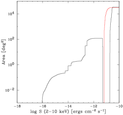
Figure 1.— Survey area plotted against limiting flux in the hard (left) and soft (right) bands. The red curve in the left panel corresponds to that of the Swift/BAT survey assuming $\gamma=1.6$.

Figure 2.— Observed source counts in the hard (left) and soft (right) bands.

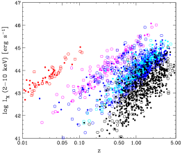
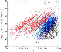
Figure 3.— Left: redshift-luminosity plot of our sample detected in the hard ($>$2 keV) band (red: Swift/BAT sample, magenta: ASCA sample, blue: XMM-Newton sample, cyan: CLASX and CLANS sample, black: CDFN and CDFS sample). The open and filled circles represent X-ray type-1 AGNs (with log $N_{\rm H}$ $<$ 22) and X-ray type-2 AGNs (with log $N_{\rm H}$ $\geq$22), respectively. Right: redshift-luminosity plot of our sample detected in the soft (0.5–2 keV) band (red: ROSAT sample, blue: XMM-Newton sample, cyan: CLANS sample, black: CDFN and CDFS sample).

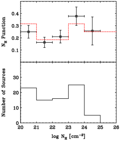
Figure 4.— Observed histogram of $N_{\rm H}$ in the Swift/BAT sample (lower) and estimated $N_{\rm H}$ function corrected for detection biases (upper). The red lines represent an example of $N_{\rm H}$ function we adopt.

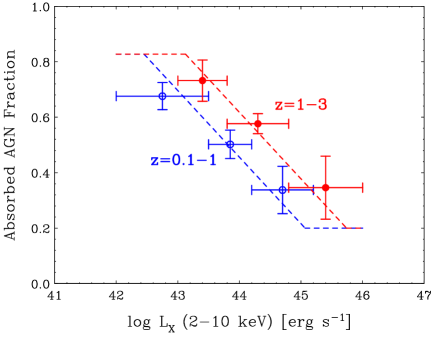
Figure 5.— Absorbed fraction of AGNs plotted against luminosity at $z=0.1-1$ (blue) and $z=1-3$ (red) as determined from the Swift/BAT, AMSS, and SXDS (hard band) samples. The dashed lines represent the best-fit models calculated at the mean redshifts for the $z=0.1-1$ and $z=1-3$ samples.

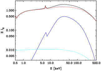
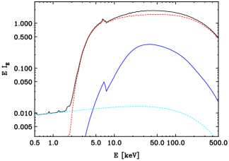
Figure 6.— Examples of the template broad band X-ray spectra (in $EI(E)$, where $E$ is energy and $I(E)$ is the energy flux) for AGNs with log $N_{\rm H}$ = 21 and $\Gamma=1.94$ (left) and log $N_{\rm H}$ = 23 and $\Gamma=1.84$ (right). Units are arbitrary. The black curve denotes the total spectrum, the red curve the transmitted continuum plus its reflection component from the torus, the blue curve the reflection component from the accretion disk, and the cyan curve the scattered component.

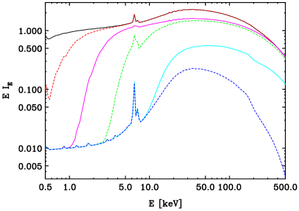
Figure 7.— Model spectra of AGNs with different absorptions (from top to bottom, log $N_{\rm H}$ = 20.5, 21.5, 22.5, 23.5, 24.5, 25.5). Units are arbitrary in $EI(E)$. A same photon index ($\Gamma=1.9$) and a normalization are assumed for the intrinsic cutoff power-law continuum in all the spectra.

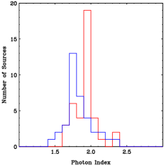
Figure 8.— Distribution of photon index for type-1 (red) and type-2 (blue) AGNs as determined from the Swift/BAT survey.

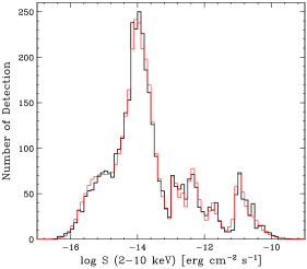
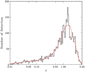
Figure 9.— Observed histograms (thick, black) of flux (left) and redshift (right) of our sample compared with model predictions (thin, red).

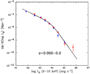
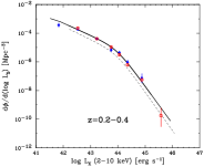
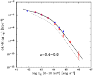
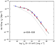
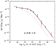
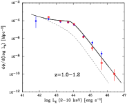
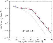
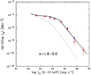
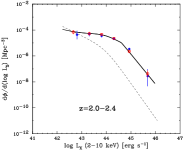
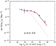
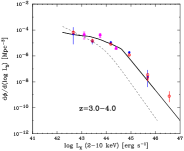
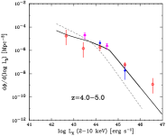
Figure 10.— De-absorbed, rest frame 2–10 keV XLF of AGNs at different redshift ranges (CTN AGNs only). The solid curve represents the best-fit XLF at the central redshift in each $z$ bin. The dashed curve is that in the local universe. Blue (red) data points are plotted according to the “$N^{\rm obs}/N^{\rm mdl}$ method” with 1$\sigma$ Poisson errors by using the hard (soft) band sample. The magenta points in the $z=3.0-4.0$ and $z=4.0-5.0$ panels are taken from Fiore et al. (2012).

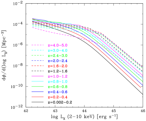
Figure 11.— Comparison of the best-fit XLF shape between different redshifts (CTN AGNs only).

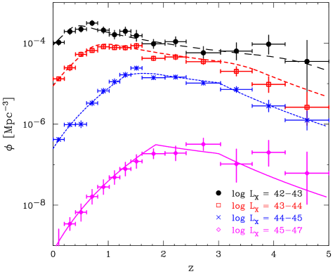
Figure 12.— Comoving number density of AGNs plotted against redshift in different luminosity bins (CTN AGNs only). The curves are the best-fit model, and the data points are calculated from either the soft or hard band sample (see Section 6).

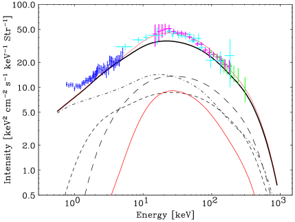
Figure 13.— XRB spectrum calculated from our AGN population synthesis model (upper solid curve, red) compared with the observed data by various missions (Ajello et al., 2008). Middle solid curve (black): the integrated spectrum of CTN AGNs (log $N_{\rm H}$ $<$24). Lower solid curve (red): that of CTK AGNs (log $N_{\rm H}$ = 24–26). Long-dashed curve (black): that of AGNs with log $N_{\rm H}$ = 23–24. Short-dashed curve (black): that of AGNs with log $N_{\rm H}$ = 22–23. Dot-dashed curve (black): that of AGNs with log $N_{\rm H}$ $<$22. Data points in the 0.8–5 keV (blue), 4–215 keV (cyan), 14–195 keV (magenta), and 100–300 keV (green) bands refer to the XRB spectra observed with ASCA/SIS (Gendreau et al., 1995), INTEGRAL (Churazov et al., 2007), Swift/BAT (Ajello et al., 2008), and HEAO1 A4 (Gruber et al., 1999), respectively.

Figure 14.— Left: contour plot showing the contribution of all (CTN+CTK) AGNs per unit $z$ and log $L_{\rm X}$ to the 2–10 keV XRB. The intervals are constant in linear scale. Right: the same but for the 10–40 keV XRB.

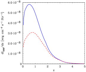
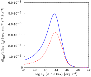
Figure 15.— Left: Differential contribution to the 2–10 keV (red dashed) or 10–40 keV (blue solid) XRB intensity as a function of redshift (in units of per $z$) from all (CTN+CTK) AGNs with log $L_{\rm X}$ = 41–47. Right: that as a function of luminosity (in units of per log $L_{\rm X}$) from all AGNs at $z=0.002-5$.

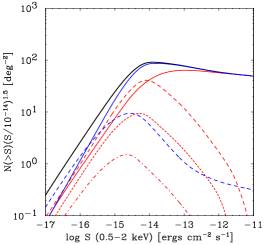
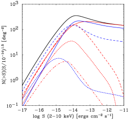
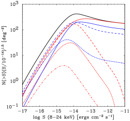
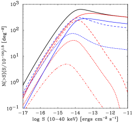
Figure 16.— upper left: predicted integrated log $N$ - log $S$ relations in the 0.5–2 keV band from our baseline model normalized as $N(>S)(S/10^{-14})^{1.5}$. The red curves correspond to those in different redshifts (solid: $z<1$, long-dashed: $z=1-2$, short-dashed: $z=2-3$, dot-dashed $z=3-5$), and blue curves to those with different absorptions (solid: log $N_{\rm H}$ = 20–22, long-dashed: log $N_{\rm H}$ = 22–24, short-dashed: log $N_{\rm H}$ = 24–26). top right: the same but for the 2–10 keV band. lower left: the same but for the 8–24 keV band. lower right: the same but for the 10–40 keV band.

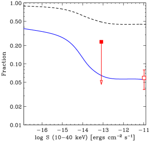
Figure 17.— Left: fractions of CTK AGNs (log $N_{\rm H}$ = 24–26, solid blue) and obscured AGNs (log $N_{\rm H}$ = 22–26, dashed black) in the total AGNs given as a function of flux in the 2–10 keV band, predicted from our baseline model. The data points correspond to the observed CTK AGN fractions by Brightman & Ueda (2012) (filled circle), Brunner et al. (2008) (open circle), Tozzi et al. (2006) (filled square), and Hasinger et al. (2007) (open square), from left to right. Here the result by Brightman & Ueda (2012) is plotted by converting the 0.5–8 keV flux to the 2–10 keV one by assuming a photon index of 1.4. Right: the same but for the 10–40 keV flux. The arrow denotes the 90% confidence upper limit of the CTK fraction obtained by NuSTAR in the 8–24 keV band (Alexander et al., 2013), and the right data point is that from the Swift/BAT 9-month survey in the 14–195 keV band (Tueller et al., 2008; Ichikawa et al., 2012). The fluxes are converted into the 10–40 keV band by assuming a photon index of 1.8.

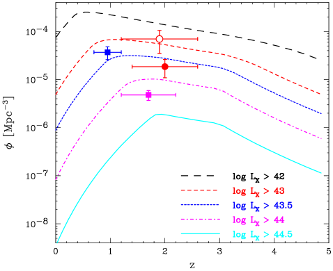
Figure 18.— Comoving number density of CTK AGNs with different lower limits for the X-ray luminosity predicted from our baseline model. The data points represent the estimates by Alexander et al. (2011) for log $L_{\rm X}$ $\lower 2.15277pt\hbox{$\;\buildrel>\over{\sim}\;$}43$ (filled circle, red), Fiore et al. (2008) for log $L_{\rm X}$ $>43$ (open circle, red), and Fiore et al. (2009) for log $L_{\rm X}$ $>43.5$ (filled square, blue) and for log $L_{\rm X}$ $>44$ (filled square, magenta).

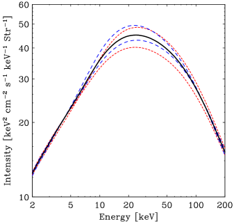
Figure 19.— The predicted XRB spectra by assuming different fractions of CTK AGN relative to obscured CTN AGNs (short-dashed, red; $f_{\rm CTK}$ = 2 and 0.5 from upper to lower), or different reflection strengths from the accretion disk (long-dashed, blue; $R_{\rm disk}$ = 1.0 and 0.25 from upper to lower). The baseline model ($f_{\rm CTK}$ = 1.0 and $R_{\rm disk}$ = 0.5) is plotted by the solid line (solid, black).

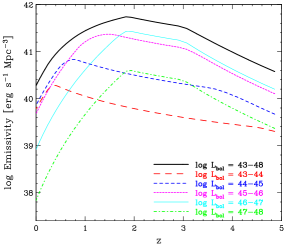
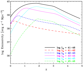
Figure 20.— Left: comoving bolometric luminosity density (emissivity) in different luminosity ranges calculated from our baseline model. Right: that in the 2–10 keV band.

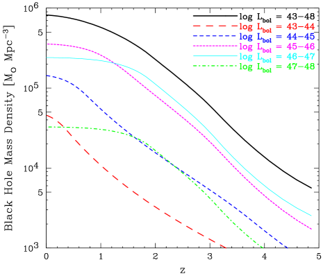
Figure 21.— Comoving mass density of all SMBHs plotted against redshift (uppermost solid curve, black). Those calculated within limited luminosity ranges are separately shown. The averaged radiation efficiency of $\overline{\eta}=0.05$ is assumed.

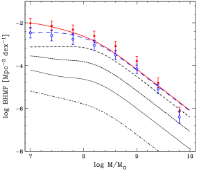
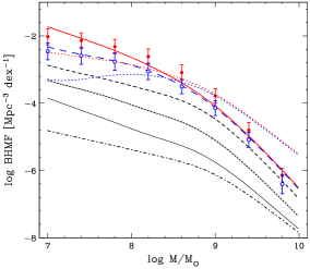
Figure 22.— Left: the curves represent AGN relic mass functions of SMBHs calculated from the continuity equation with a constant radiation efficiency of $\eta=0.091$ and an averaged Eddington ratio of log $\overline{\lambda}=0.07$ at $z=5$ (dot-dashed, black), $z=4$ (thin solid, black), $z=3$ (short-dashed, black), $z=2$ (med-dashed, black), $z=1$ (long-dashed, blue), and $z=0$ (thick solid, red). The filled circles (red) and open circles (blue) represent the observed SMBH mass functions at $z=0$ and $z=1$, respectively, sampled from Li et al. (2011). Right: the same but with a mass-dependent radiation efficiency in the form of $\eta=0.093(M/10^{8}\mbox{${M_{\odot}}$})^{0.42}$ and an averaged Eddington ratio of log $\overline{\lambda}=-0.6$. The lower (blue) and upper (red) dotted curves represent the best-fit results with a constant radiation efficiency and log $\overline{\lambda}=-0.6$.

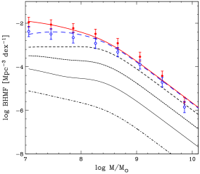
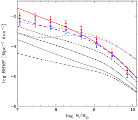
Figure 23.— Left: the curves represent AGN relic mass functions of SMBHs calculated from the continuity equation with a constant radiation efficiency of $\eta=0.053$ and an averaged Eddington ratio of log $\overline{\lambda}=-0.014$ at $z=5$ (dot-dashed, black), $z=4$ (thin solid, black), $z=3$ (short-dashed, black), $z=2$ (med-dashed, black), $z=1$ (long-dashed, blue), and $z=0$ (thick solid, red). The filled circles (red) and open circles (blue) represent the SMBH mass functions at $z=0$ and $z=1$, respectively, revised from the Li et al. (2011) data with the updated calibration between SMBH mass and bulge mass by Kormendy & Ho (2013). Right: the same but with a mass-dependent radiation efficiency in the form of $\eta=0.043(M/10^{8}\mbox{${M_{\odot}}$})^{0.54}$ and an averaged Eddington ratio of log $\overline{\lambda}=-1.1$. The lower (blue) and upper (red) dotted curves represent the best-fit results with a constant radiation efficiency and log $\overline{\lambda}=-1.1$.

Table 1Surveys Used in the Analysis

Survey	Energy Band	Flux Limit ($\Gamma$)	Area	No. of AGNs	Completeness	Reference
	(keV)	(erg cm-2 s-1)	(deg2)		(%)
BAT9	14–195	$8.4\times 10^{-12}$ (1.6)	30500	87 (85)	100	(1)
MAXI7	4–10	$2.4\times 10^{-11}$ (1.6)	34000	38 (37)	99	(2)
AMSS	2–10	$3.1\times 10^{-13}$ (1.6)	90.8	95 (95)	97	(3)
ALSS	2–7	$1.2\times 10^{-13}$ (1.6)	5.56	30 (30)	100	(4)
SXDS	2–10	$2.7\times 10^{-15}$ (1.2)	1.02	569 (567)	99	(5)
SXDS	0.5–2	$6.8\times 10^{-16}$ (1.4)	1.02	725 (703)	99	(5)
LH/XMM	2–4.5	$6.1\times 10^{-15}$ (1.2)	0.183	57 (57)	91	(6)
LH/XMM	0.5–2	$1.3\times 10^{-15}$ (1.4)	0.126	58 (57)	88	(7)
H2X	2–10	$1.7\times 10^{-14}$ (1.2)	0.90	87 (87)	92	(8)
HBSS	4.5–7.5	$2.2\times 10^{-13}$ (1.6)	25.17	62 (62)	97	(9)
CLASXS	2–8	$1.9\times 10^{-14}$ (1.2)	0.280	50 (50)	96	(10)
CLANS	2–8	$1.0\times 10^{-14}$ (1.2)	0.490	159 (158)	95	(10,11)
CLANS	0.5–2	$2.3\times 10^{-15}$ (1.4)	0.490	191 (183)	95	(10,11)
CDFN	2–8	$2.1\times 10^{-16}$ (1.0)	0.124	307 (298)	100	(6,10)
CDFN	0.5–2	$2.8\times 10^{-17}$ (1.4)	0.124	402 (234)	100	(7,10)
CDFS	2–8	$1.1\times 10^{-16}$ (1.0)	0.129	358 (347)	95	(12)
CDFS	0.5–2	$1.1\times 10^{-17}$ (1.4)	0.129	583 (299)	93	(12)
ROSAT	0.5–2	$3.5\times 10^{-14}$ (1.8)	0.3–21400	722 (705)	99	(7)

References. — (1) Tueller et al. (2008); (2) Ueda et al. (2011); (3) Akiyama et al. (2003); (4) Akiyama et al. (2000); (5) Akiyama et al. (2013); (6) Hasinger (2008) and references therein; (7) Hasinger et al. (2005) and references therein; (9) Della Ceca et al. (2008); (10) Trouille et al. (2008); (11) Trouille et al. (2009); (12) Xue et al. (2011);

Table 2Parameters of Absorption Function

$\psi_{43.75}^{0}$	$\beta$	$\psi_{\rm min}$	$\epsilon$	$a1$	$f_{\rm CTK}$
0.43$\pm$0.03	0.24 (fixed)	0.2 (fixed)	1.7 (fixed)	0.48$\pm$0.05	1.0 (fixed)

Note. — Errors are 1$\sigma$ for a single parameter.

Table 3Parameters of Photon Index Function

$\overline{\Gamma_{1}}$	$\Delta\Gamma_{1}$	$\overline{\Gamma_{2}}$	$\Delta\Gamma_{2}$
1.94$\pm$0.03	0.09$\pm$0.05	1.84$\pm$0.04	0.15$\pm$0.06

Note. — Attached errors (1$\sigma$) are based on the Swift/BAT 9-month sample. These are fixed at the best-fit values when performing ML fit to the whole sample (Section 6).

Table 4Best Fit Parameters of AGN Luminosity Functions

Band	$A$	log $L_{*}$	$\gamma_{1}$	$\gamma_{2}$	$p1^{*}$	$\beta_{1}$	$z_{\rm c1}^{*}$	log $L_{\rm a1}$	$\alpha_{1}$
2–10 keV	2.91$\pm$0.07	43.97$\pm$0.06	0.96$\pm$0.04	2.71$\pm$0.09	4.78$\pm$0.16	0.84$\pm$0.18	1.86$\pm$0.07	44.61$\pm$0.07	0.29$\pm$0.02
bolometric	3.26$\pm$0.08	45.48$\pm$0.09	0.89$\pm$0.03	2.13$\pm$0.07	5.33$\pm$0.15	0.46$\pm$0.15	1.86	46.20$\pm$0.04	0.29

Note. — Errors are 1$\sigma$ for a single parameter. Only free parameters are listed for the XLF; we fix $p2=-1.5$, $p3=-6.2$, $z_{\rm c2}^{*}=3.0$, log $L_{\rm p}$ = log $L_{\rm a2}=44(45.67)$ for the XLF (BLF), and $\alpha 2=-0.1$ (see Section 6).

Table 5Comparison of Model Predictions

Changed Parameters	$a1$	$I_{\rm XRB,20-50}$	$N(>S)$
		($10^{-8}$ erg cm-2 s-1 Str-1)	(deg-2)
baseline model	0.48$\pm$0.05	6.39	4300
$f_{\rm CTK}=2.0$	0.34$\pm$0.08	6.87	4500
$f_{\rm CTK}=0.5$	0.55$\pm$0.06	5.72	4120
$R_{\rm disk}=1.0$	0.39$\pm$0.07	6.91	4280
$R_{\rm disk}=0.25$	0.54$\pm$0.06	6.13	4320
$\overline{\Gamma_{1}}=1.97$ and $\overline{\Gamma_{2}}=1.88$	0.51$\pm$0.06	5.88	4270
$\overline{\Gamma_{1}}=1.91$ and $\overline{\Gamma_{2}}=1.80$	0.44$\pm$0.07	6.91	4330
$\Delta\Gamma_{1}=0.14$ and $\Delta\Gamma_{2}=0.21$	0.48$\pm$0.05	6.82	4340
$\Delta\Gamma_{1}=0.04$ and $\Delta\Gamma_{2}=0.10$	0.46$\pm$0.06	6.09	4230

Note. — The other parameters are the same as in the baseline model.

Table 6Summary of Population Synthesis Models

References	XLF	$a1$	$\overline{\Gamma}$	$\Delta\Gamma$	$E_{\rm c}$	$f_{\rm CTK}$ (log $N_{\rm H}$)	$R_{total}$	$EI_{\rm XRB}(E)$ at 30 keV
					(keV)			(keV cm-2 s-1 Str-1)
(1)	U03	0	1.9	0	500	0.63 (24–25)	1.0	50
(2)	U03	0.3	1.9	0	375	0.5 (24–25)	1.0	52
(3)	H05	0	1.9	0.2	200	1.05 (24–26)	$\approx$1.0	40
(4)	U03	0.4	1.9	0	300	0.17 (24–26)	1.2	42
(5)	U03	0	1.88	0.15	230	0.1 (24–25)	$\approx$1.0	44
this work	this work	0.48	1.94, 1.88	0.09, 0.15	300	1.0 (24–26)	0.5+$R_{\rm torus}$	45

References. — (1) Ueda et al. (2003); (2) Ballantyne et al. (2006); (3) Gilli et al. (2007); (4) Treister et al. (2009); (5) Akylas et al. (2012)

References

- Aird et al. (2010) Aird, J. et al. 2010, MNRAS, 401, 2531
- Ajello et al. (2008) Ajello, M. et al. 2008, ApJ, 689, 666
- Akiyama et al. (2000) Akiyama, M., et al. 2000, ApJ, 532, 700
- Akiyama et al. (2003) Akiyama, M., Ueda, Y., Ohta, K., Takahashi, T., & Yamada, T. 2003, ApJS, 148, 275
- Akiyama et al. (2013) Akiyama, M. et al. 2014, in prep.
- Akylas et al. (2012) Akylas, A., Georgakakis, A., Georgantopoulos, I., Brightman, M., Nandra, K. 2012, A&A, 546, 98
- Alexander et al. (2003) Alexander, D.M. et al. 2003, AJ, 126, 539
- Alexander et al. (2011) Alexander, D.M. et al. 2011, ApJ, 738, 44
- Alexander et al. (2013) Alexander, D.M. et al. 2013, ApJ, 773, 125
- Appenzeller et al. (1998) Appenzeller, I. et al. 1998, ApJS, 117, 319
- Baldi et al. (2002) Baldi, A., Molendi, S., Comastri, A., Fiore, F., Matt, G., & Vignali, C. 2002, ApJ, 564, 190
- Ballantyne et al. (2006) Ballantyne, D.R., Everett, J.E., Murray, N. 2006, ApJ, 639, 740
- Ballantyne (2014) Ballantyne, D.R. 2014, MNRAS, 437, 2845
- Barcons et al. (2000) Barcons, X., Mateos, S., & Ceballos, M.T. 2000, MNRAS, 316, L13
- Barcons et al. (2007) Barcons, X. et al. 2007, A&A, 476, 1191
- Barger et al. (2001) Barger, A.J., Cowie, L.L., Bautz, M.W., Brandt, W.N., Garmire, G.P., Hornschemeier, A.E., Ivison, R.J., & Owen, F.N. 2001, AJ, 122, 2177
- Barger et al. (2003) Barger, A.J. et al. 2003, AJ, 126, 632
- Barger et al. (2005) Barger, A.J. et al. 2005, AJ, 129, 578
- Beckmann et al. (2009) Beckmann, V. et al. 2009, A&A, 505, 417
- Boyle et al. (1993) Boyle, B.J. et al. 1993, MNRAS, 260, 49
- Brandt & Hasinger (2005) Brandt, W.N., & Hasinger, G. 2005, ARA&A, 43, 827
- Brightman & Nandra (2011a) Brightman, M., & Nandra, K. 2011, MNRAS, 413, 1206
- Brightman & Nandra (2011b) Brightman, M., & Nandra, K. 2011, MNRAS, 414, 3084
- Brightman & Ueda (2012) Brightman, M., & Ueda, Y. 2012, MNRAS, 423, 702
- Brunner et al. (2008) Brunner, H., Cappelluti, N., Hasinger, G., Barcons, X., Fabian, A.C., Mainieri, V., & Szokoly, G. 2008, A&A, 479, 283
- Brusa et al. (2009) Brusa, M., et al. 2009, ApJ, 693, 8
- Burlon et al. (2011) Burlon, D., Ajello, M., Greiner, J., Comastri, A., Merloni, A., & Gehrels, N. 2011, ApJ, 728, 58
- Cao & Li (2008) Cao, X.-W., & Li, F. 2008, MNRAS, 390, 561
- Chapman et al. (2005) Chapman, S.C., Blain, A.W., Smail, I., Ivison, R.J. 2005, ApJ, 622, 772
- Churazov et al. (2007) Churazov, E. et al. 2007, A&A, 467, 529
- Civano et al. (2011) Civano, F., et al. 2011, ApJ, 741, 91
- Cocchia et al. (2007) Cocchia, F. et al. 2007, A&A, 466, 31
- Cohen et al. (2000) Cohen, J.G., Hogg, D.W., Blandford, R., Cowie, L.L., Hu, E., Songaila, A., Shopbell, P., & Richberg, K. 2000, ApJ, 538, 29
- Comastri et al. (1995) Comastri, A., Setti, G., Zamorani, G., & Hasinger, G. 1995, A&A, 296, 1
- Cowie et al. (1996) Cowie, L.L., Songaila, A., Hu, E.M., & Cohen, J.G. 1996, AJ, 112, 839
- Daddi et al. (2007) Daddi, E. 2007 et al. 2007, ApJ, 670, 173
- Dadina (2008) Dadina, M. 2008, A&A, 485, 417
- Della Ceca et al. (2004) Della Ceca, R. et al. 2004, A&A, 428, 383
- Della Ceca et al. (2008) Della Ceca, R. et al. 2008, A&A, 487, 119
- De Luca & Molendi (2004) De Luca, A., & Molendi, S. 2004, A&A, 419, 837
- Draper & Ballantyne (2009) Draper, A.R., & Ballantyne, D.R. 2009, ApJ, 707, 778
- Ebrero et al. (2009) Ebrero, J. et al. 2009, A&A, 493, 55
- Eckart et al. (2006) Eckart, M.E., Stern, D., Helfand, D.J., Harrison, F.A., Mao, P.H., & Yost, S.A. 2006, ApJS, 165, 19
- Eguchi et al. (2009) Eguchi, S., Ueda, Y., Terashima, Y., Mushotzky, R., & Tueller, J. 2009, ApJ, 696, 1657
- Eguchi et al. (2011) Eguchi, S., Ueda, Y., Awaki, H., Aird, J., Terashima, Y., & Mushotzky, R. ApJ, 729, 31
- Ferrarese & Merritt (2000) Ferrarese, L., & Merritt, D. 2000, ApJ, 539, L9
- Fiore et al. (2003) Fiore, F. et al. 2003, A&A, 409, 79
- Fiore et al. (2008) Fiore, F. et al. 2008, ApJ, 672, 94
- Fiore et al. (2009) Fiore, F. et al. 2009, ApJ, 693, 447
- Fiore et al. (2012) Fiore, F. et al. 2012, A&A, 537, 16
- Fontanot et al. (2009) Fontanot, F., De Lucia, G., Monaco, P., Somerville, R.S., & Santini, P. 2009, MNRAS, 397, 1776
- Fotopoulou et al. (2012) Fotopoulou, S. et al. 2012, ApJS, 198, 1
- Fronetera et al. (2007) Frontera, F. et al. 2007, ApJ, 666, 86
- Fukazawa et al. (2011) Fukazawa, Y. et al. 2011, ApJ, 727, 19
- Furusawa et al. (2008) Furusawa, H. et al. 2008, ApJS, 176, 1
- Gebhardt et al. (2000) Gebhardt, K., et al. 2000, ApJ, 539, L13
- Gehrels (1986) Gehrels, N. 1986, ApJ, 303, 336
- Gendreau et al. (1995) Gendreau, K.C. et al. 1995, PASJ, 47, L5
- Giacconi et al. (2002) Giacconi, R., et al. 2002, ApJS, 139, 369
- Gilli et al. (1999) Gilli, R., Risaliti, G., & Salvati, M. 1999, A&A, 347, 424
- Gilli et al. (2007) Gilli, R., Comastri, A., & Hasinger, G. 2007, A&A, 463, 79
- Gioia et al. (2003) Gioia, I.M., Henry, J.P., Mullis, C.R., Böhringer, H., Briel, U.G., Voges, W., & Huchra, J.P. 2003, ApJS, 149, 29
- Grossan (1992) Grossan, B., 1992, PhD thesis, MIT
- Gruber et al. (1999) Gruber, D.E., et al. 1999, ApJ, 520, 124
- Gültekin et al. (2009) Gültekin, K. et al. 2009, ApJ, 698, 198
- Häring & Rix (2004) Häring, N., & Rix, H. 2004, ApJ, 604, L89
- Hasinger et al. (2001) Hasinger, G. et al. 2001, A&A, 365, L45
- Hasinger et al. (2005) Hasinger, G., Miyaji, T., & Schmidt, M. 2005, A&A, 441, 417 (H05)
- Hasinger et al. (2007) Hasinger, G. et al. 2007, ApJS, 172, 29
- Hasinger (2008) Hasinger, G. 2008, A&A, 490, 905
- Hiroi et al. (2011) Hiroi, K. et al. 2011, PASJ, 63S, 677
- Hiroi et al. (2012) Hiroi, K., Ueda, Y., Akiyama, M., & Watson, M.G. 2012, ApJ, 758, 49
- Hopkins et al. (2007) Hopkins, P. F., Hernquist, L., Cox, T. J., Robertson, B., & Krause, E. 2007, ApJ, 669, 67
- Ichikawa et al. (2012) Ichikawa, K. et al. 2012, ApJ, 754, 45
- Ikeda et al. (2009) Ikeda, S., Awaki, H., & Terashima, Y. 2009, ApJ, 692, 608
- Iwasawa & Taniguchi (1993) Iwasawa, K., & Taniguchi, Y. 1993, ApJ, 413, L15
- Iwasawa et al. (2012) Iwasawa, K. et al. 2012, A&A, 546, 84
- Jones et al. (1997) Jones, L.R., et al. 1997, MNRAS, 285, 547
- Kelly & Shen (2013) Kelly, B.C., & Shen, Y. 2013, ApJ, 764, 45
- Kodama et al. (2004) Kodama, T. et al. 2004, MNRAS, 350, 1005
- Kollmeier et al. (2006) Kollmeier et al. 2006, ApJ, 648, 128
- Kormendy & Bender (2009) Kormendy, J., & Bender, R. 2009, ApJ, 691, L142
- Kormendy & Ho (2013) Kormendy, J., & Ho, L.C. 2013, ARA&A, 51, 511
- La Franca et al. (2005) La Franca, F. et al. 2005, ApJ, 635, 864
- Lehmer et al. (2010) Lehmer, B.D. et al. 2010, ApJ, 724, 559
- Lehmer et al. (2012) Lehmer, B.D. et al. 2012, ApJ, 752, 46
- Li et al. (2011) Li, Y.-R., Ho, L.C., & Wang,J.-M. 2011, ApJ, 742, 33
- Li et al. (2012) Li, Y.-R., Wang,J.-M. & Ho, L.C., 2012, ApJ, 749, 187
- Maccacaro et al. (1991) Maccacaro, T. et al. 1991, ApJ, 374, 117
- Magdziarz & Zdziarski (1995) Magdziarz, P., & Zdziarski, A.A. 1995, MNRAS, 273, 837
- Magorrian et al. (1998) Magorrian, J., et al. 1998, AJ, 115, 2285
- Maiolino et al. (2006) Maiolino, R. et al. 2006, A&A, 445, 457
- Malizia et al. (2009) Malizia, A, Stephen, J.B., Bassani, L., Bird, A.J., Panessa, F., Ubertini, P. 2009, MNRAS, 399, 944
- Marconi & Hunt (2003) Marconi, A., & Hunt, L.K. 2003, ApJ, 589, L21
- Marconi et al. (2004) Marconi, A., Risaliti, G., Gilli, R., Hunt, L.K., Maiolino, R., & Salvati, M. 2004, MNRAS, 351, 169
- Marshall et al. (1980) Marshall, F.E., et al. 1980, ApJ, 1980, 235, 4
- Mason et al. (2000) Mason, K.O. et al. 2000, MNRAS, 311, 456
- Mateos et al. (2005) Mateos, S., Barcons, X., Carrera, F.J., Ceballos, M.T., Hasinger, G., Lehmann, I., Fabian, A.C., & Streblyanska, A. 2005, A&A, 444, 79
- Matsuoka et al. (2009) Matsuoka, M. et al. 2009, PASJ, 61, 999
- Mignoli et al. (2004) Mignoli, M. et al. 2004, A&A, 418, 827
- Miyaji et al. (2000) Miyaji, T., Hasinger, G., & Schmidt, M. 2000, A&A, 353, 25
- Miyaji et al. (2001) Miyaji, T., Hasinger, G., & Schmidt, M. 2001, A&A, 369, 49
- Mullis et al. (2004) Mullis, C.R., Henry, J.P., Gioia, I.M., Böhringer, H., Briel, U.G., Voges, W., & Huchra, J.P. 2004, ApJ, 617, 192
- Nobuta et al. (2012) Nobuta et al. 2012, ApJ, 761, 143
- Novak (2014) Novak, G.S. 2014, submitted to MNRAS (arXiv:1310.3833)
- Page et al. (1997) Page, M.J., Mason, K.O., McHardy, I.M., Jones, L.R., & Carrera, F.J. 1997, MNRAS, 291, 324
- Paolillo et al. (2004) Paolillo, M., Schreier, E.J., Giacconi, R., Koekemoer, A.M., Grogin, N.A. 2004, ApJ, 611, 93
- Persic & Raphaeli (2002) Persic, M. & Rephaeli, Y. 2002, A&A, 382, 843
- Perola et al. (2004) Perola, G.C. et al. 2004, A&A, 421, 491
- Piccinotti et al. (1982) Piccinotti, G., et al. 1982, ApJ, 253, 485
- Reddy et al. (2006) Reddy, N.A., Steidel, C.C., Erb, D.K., Shapley, A.E., & Pettini, M. 2006, ApJ, 653, 1004
- Ricci et al. (2013) Ricci, C., Paltani, S., Awaki, H., Petrucci, P.-O., Ueda, Y., & Brightman, M. 2013, A&A, 553, 29
- Risaliti et al. (1999) Risaliti, G., Maiolino, R., & Salvati, M. 1999, ApJ, 522, 157
- Shinozaki et al. (2006) Shinozaki, K., Miyaji, T., Ishisaki, Y., Ueda, Y., & Ogasaka, Y. 2006, AJ, 131, 2843
- Silverman et al. (2005) Silverman, J.D. et al. 2005, ApJ, 624, 630
- Silverman et al. (2008) Silverman, J.D. et al. 2008, ApJ, 679, 118
- Schwope et al. (2000) Schwope, A. et al. 2000, AN, 321. 1
- Scoville et al. (2007) Scoville, N. et al. 2007, ApJS, 172, 1
- Shankar et al. (2004) Shankar, F., Salucci, P., Granato, G.L., De Zotti, G., & Danese, L. 2004, MNRAS, 354, 1020
- Shankar et al. (2009) Shankar, F., Weinberg, D.H., Miralda-Escudé, J. 2009, ApJ, 690, 20
- Shankar et al. (2013) Shankar, F., Weinberg, D.H., Miralda-Escudé, J. 2013, MNRAS, 428, 421
- Simpson (2005) Simpson, C. 2005, MNRAS, 360, 565
- Small & Blandford (1992) Small, T.A., & Blandford, R.D. 1992, MNRAS, 259, 725
- Soltan (1982) Soltan, A. 1982, MNRAS, 200, 115
- Steffen et al. (2003) Steffen, A.T., Barger, A.J., Cowie, L.L., Mushotzky, R.F., & Yang, Y. 2003, ApJ, 596, L23
- Steffen et al. (2004) Steffen, A.T., Barger, A.J., Capak, P., Cowie, L.L., Mushotzky, R.F., & Yang, Y. 2004, AJ, 128, 1483
- Swinbank et al. (2004) Swinbank, A.M., Smail, I., Chapman, S.C., Blain, A.W., Ivison, R.J., & Keel, W.C. 2004, ApJ, 617, 64
- Tamura et al. (2006) Tamura, N., Ohta, K., & Ueda, Y. 2006, MNRAS, 365, 134
- Tozzi et al. (2006) Tozzi, P. et al. 2006, A&A, 451, 457
- Treister & Urry (2005) Treister, E., & Urry, C.M. 2005, ApJ, 630, 115
- Treister & Urry (2006) Treister, E., & Urry, C.M. 2006, ApJ, 652, L79
- Treister et al. (2009) Treister, E., Urry, C.M., & Virani, S. 2009, ApJ, 696, 110
- Trouille et al. (2008) Trouille, L., Barger, A.J., Cowie, L.L., Yang, Y., & Mushotzky, R.F. 2008, ApJS, 179, 1
- Trouille et al. (2009) Trouille, L., Barger, A.J., Cowie, L.L., Yang, Y., & Mushotzky, R.F. 2009, ApJ, 703, 2160
- Tueller et al. (2008) Tueller, J., et al. 2008, ApJ, 681, 113
- Ueda et al. (1998) Ueda, Y., et al. 1998, Nature, 391, 866
- Ueda et al. (1999) Ueda, Y., et al. 1999, ApJ, 518, 656
- Ueda et al. (2001) Ueda, Y., Ishisaki, Y., Takahashi, T., Makishima, K., & Ohashi, T. 2001, ApJS, 133, 1
- Ueda et al. (2003) Ueda, Y., Akiyama, M., Ohta, K., & Miyaji, T. 2003, ApJ, 598, 886 (U03)
- Ueda et al. (2005) Ueda, Y., Ishisaki, Y., Takahashi, T., Makishima, K., & Ohashi, T. 2005, ApJS, 161, 185
- Ueda et al. (2008) Ueda, Y. et al. 2008, ApJS, 179, 124
- Ueda et al. (2011) Ueda, Y. et al. 2011, PASJ, 63S, 937
- Vasudevan et al. (2013) Vasudevan, R.V., Brandt, W.N., Mushotzky, R.F., Winter, L.M., Baumgartner, W.H., Shimizu, T.T., Schneider, D.P., & Nousek, J. 2013, ApJ, 763, 111
- Vika et al. (2009) Vika, M., Driver, S.P., Graham, A.W. Liske, J. 2009, MNRAS, 400, 1451
- Vito et al. (2013) Vito, F. et al. 2013, MNRAS, 428, 354
- Wilman & Fabian (1999) Wilman, R.J., & Fabian, A.C. 1999, MNRAS, 309, 862
- Winter et al. (2009a) Winter, L.M., Mushotzky, R.F., Reynolds, C.S., & Tueller, J. 2009, ApJ, 690, 1322
- Winter et al. (2009b) Winter, L.M., Mushotzky, R.F., Terashima, Y., & Ueda, Y. 2009, ApJ, 701, 644
- Xue et al. (2011) Xue, Y.Q. et al. 2011, ApJS, 195, 10
- Yang et al. (2004) Yang, Y., Mushotzky, R.F., Steffen, A.T., Barger, A.J., & Cowie, L.L. 2004, AJ, 128, 1501
- Yencho et al. (2009) Yencho, B., Barger, A.J., Trouille, L., & Winter, L.M. 2009, ApJ, 698, 380
- Yu & Tremeine (2012) Yu, Q., & Tremeine, S. 2002, MNRAS, 335, 965
- Zdziarski et al. (1995) Zdziarski, A.A., et al. 1995, ApJ, 438, L63
- Zdziarski et al. (2000) Zdziarski, A.A., Poutanen, J., & Johnson W.N. 2000, ApJ, 542, 703