Turbulence on hyperbolic plane:
the fate of inverse cascade
Abstract
We describe ideal incompressible hydrodynamics on the hyperbolic plane which is an infinite surface of constant negative curvature. We derive equations of motion, general symmetries and conservation laws, and then consider turbulence with the energy density linearly increasing with time due to action of small-scale forcing. In a flat space, such energy growth is due to an inverse cascade, which builds a constant part of the velocity autocorrelation function proportional to time and expanding in scales, while the moments of the velocity difference saturate during a time depending on the distance. For the curved space, we analyze the long-time long-distance scaling limit, that lives in a degenerate conical geometry, and find that the energy-containing mode linearly growing with time is not constant in space. The shape of the velocity correlation function indicates that the energy builds up in vortical rings of arbitrary diameter but of width comparable to the curvature radius of the hyperbolic plane. The energy current across scales does not increase linearly with the scale, as in a flat space, but reaches a maximum around the curvature radius. That means that the energy flux through scales decreases at larger scales so that the energy is transferred in a non-cascade way, that is the inverse cascade spills over to all larger scales where the energy pumped into the system is cumulated in the rings. The time-saturated part of the spectral density of velocity fluctuations contains a finite energy per unit area, unlike in the flat space where the time-saturated spectrum behaves as .
1 Introduction
Incompressible Navier-Stokes turbulence in two dimensions presents a very different phenomenology from that in three dimensions due to the presence of two different quadratic conserved quantities, the energy and the enstrophy [4, 12, 14, 20]. It has been argued in [20, 4] that this leads to two coexisting cascades: the direct one towards short distances for the enstrophy and the inverse one towards long distances for the energy. The persistence of such two cascades requires, however, special conditions of scale separation: the injection scale on which forcing keeps operating must be much longer than the dissipation scale on which viscous dissipation removes enstrophy and much shorter than the integral scale (the size of the container or friction scale) which does not allow the energy to cascade further. If only the second condition is satisfied, no enstrophy cascade will develop and a part of energy will be dissipated at short and intermediate scales, but the remaining energy will still be transferred towards longer distances in the inverse cascade. If there is no effective friction mechanism removing energy at large scales, then, upon reaching finite integral scale, the inverse cascade will start building energy at that and intermediate distances developing large-scale coherent vortical motions and, eventually, a stationary state with no cascades. Otherwise, i.e. in the infinite space or in presence of a large scale friction, the inverse cascade will persist for all times. Such a stationary inverse energy cascade seems to be the simplest turbulent state as it exhibits Kolmogorov scaling properties with no visible intermittency corrections [22, 7], unlike the direct energy cascade in three dimensions [1]. The absence of intermittency indicates possible existence of the scaling limit where the injection scale is pushed to zero and the scale-invariance holds exactly. A theoretical understanding of such a scaling state may be a challenge that is not completely out of reach. Although the existence of the scaling limit for the Navier-Stokes inverse cascade is only a plausible assumption, it is reassuring to know that there is a much simpler hydrodynamical system, the Kraichnan model of passive scalar advection, that exhibits similar features at least partly under analytic control: no intermittency in the inverse cascade and intermittency in the direct one [13].
To add to the puzzle about the Navier-Stokes inverse cascade, but possibly providing an important clue, it has been observed [5, 6] that the zero-vorticity lines seem to behave as fractal interfaces in some critical two-dimensional models of statistical mechanics (e.g. the percolation), pointing to the possible presence of a conformally invariant sector in the scaling limit of the theory (such properties have no analogue for the passive scalar [25]). Searching for a possible source of this behavior was a part of our original motivation to study the two-dimensional Navier-Stokes turbulence in different background Riemannian geometries. As all such geometries are locally conformally equivalent, comparing flows in different geometries could permit to identify better the conformally invariant features of the inverse cascade that should be present whenever the geometry supports such a turbulent state. The latter condition eliminates compact geometries (as that of a sphere), where the inverse cascade is eventually blocked. We also demand that the underlying geometry has as many symmetries as the infinite flat space, admitting an analogue of the homogeneous and isotropic turbulence. This leaves us with a single choice: that of the hyperbolic plane with constant negative curvature. Such geometry, that has the three-dimensional Lorentz group doubly covered by as the isometry group, possesses many concrete realizations. It may be viewed as a unit disc with the Poincaré metric, or as the complex upper half plane with the hyperbolic metric, or as the upper sheet of the two-sheeted hyperboloid in the three-dimensional Minkowski space with the induced metric. Different presentations may be convenient for the discussion of different aspects but are otherwise equivalent. One of the basic features of the hyperbolic geometry is that on distances longer than the curvature radius there is more room than in flat space. Suppose that we start the inverse cascade in such geometry at the forcing scale much shorter than , where the dynamics of the flow does not feel the curvature and thus should be similar to that in the flat space. In principle, such a cascade should not be blocked at scales longer than as it has more than enough room there to evolve in. The main question we address in this paper is what happens with the cascade in the hyperbolic plane at such long scales.
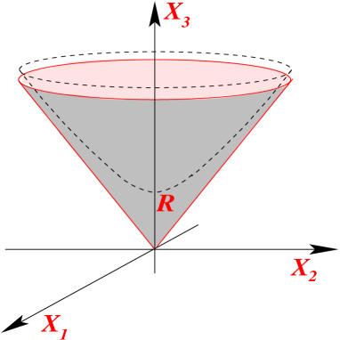
We do not have a firm answer to this question but we propose a scenario describing the long-distance, long-time fate of the inverse cascade on the hyperbolic plane that seems to pass several consistency checks. Assuming that the energy input is time-independent, we conclude that the energy density grows linearly with time. The question is then: what is the part of the 2-point velocity autocorrelation function that grows linearly in time condensing energy in it? In a flat space, it may be inferred from simple scaling that this is a constant mode that extends to longer and longer distances. Physically, it corresponds to flows that look locally as uniform jets getting longer and wider with time. On the hyperbolic plane, the exact form of such a growing-in-time mode cannot be determined by scaling because of the presence of the additional distance scale . One can only analyze its asymptotic behavior at scales much shorter than (but longer than the injection scale) or much longer than . In particular, such a mode should still be approximately constant at distances much shorter than the curvature radius. What about its behavior on distances much longer than ? We observe that on such distances the geometry of a hyperboloid in the Minkowski space looks more and more as that of the light-cone, see Figure 1, so the long distance asymptotics of the cascade might be realized by a cascade on the Minkowski light-cone.
The light-cone geometry is only semi-definite being degenerate in the light-ray directions. It has the infinite-dimensional group as the isometry group, which is also the group of conformal one-dimensional symmetries. In particular, the Euler equation in the light-cone geometry has this group as its symmetries and an infinity of related conserved quantities. We set up a formal long-distance scaling limit of the randomly forced Navier-Stokes dynamics on the hyperboloid so that, if convergent, it should determine the long-time long-distance asymptotics of the hyperbolic plane inverse cascade. We note that the complete convergence cannot take place because the scaling limit of the forcing covariance is partly singular, but even a partial convergence should fix the long-distance behavior of the energy-condensing mode, as well as that of the remaining part of the velocity 2-point function if such a remainder stabilizes with time, as in the flat space case. Both long distance behaviors are then determined by scaling. This way we find the short-distance and long-distance asymptotic behaviors of the 2-point function mode growing linearly in time. Unlike in the flat space, where the constant mode corresponds to the zero wavenumber, on the hyperbolic plane, the mode growing linearly in time contains all wave numbers. This means that after reaching the wavenumber of order , the inverse energy cascade in the wavenumber space overspills to other, in particular shorter, wavenumbers constantly feeding them with energy so that on such scales one cannot really speak of the wavenumber-space cascade in the usual sense. This is confirmed by the analysis of the flux relation in the position space. In the flat space, this relation states that the energy current across scales, expressed by a 2-point function built of three velocities, grows linearly with the distance within the inverse cascade regime, corresponding the constant energy flux through the scales. We analyze an analogous flux relation on the hyperbolic plane and show that the energy current reaches a maximum around the scale equal to the curvature radius with the energy flux changing sign there. Moreover, a properly defined velocity autocorrelation function changes sign at distances exceeding , which prompts the interpretation that the jets do not grow wider than and look like rings at larger scales, with circular motion providing velocity anti-correlation.
A word of general warning to the reader is due. Despite of the use of mathematical tools, this paper contains only a heuristic physical analysis of the Navier-Stokes turbulence in the hyperbolic plane. Not much is mathematically known about the existence and properties of a random process that solves the stochastic Navier-Stokes equations on the hyperbolic plane of the type considered here. Even in an infinite flat space, there are only weak results about such general questions [24], in contrast to the finite domains where such problems were much more studied by the mathematical community and the general questions (and more) are settled with full rigor [21]. Infinite spaces present additional difficulty as they clearly require appropriate conditions on the limits of flows at infinity for the evolution equations to be well posed, see below.
Let us briefly summarize the structure of the paper. In Sec. 2, we recall the well known Lagrangian formulation of the Euler equation on a general -dimensional Riemannian manifold. This allows us to discuss in Sec. 3 the symmetries of such equation within Noether’s approach. Sec. 4 recalls the formulation of the Navier-Stokes equation in the geometric setup. In Sec. 5, we discuss the particular case of the Euler equation on the hyperbolic plane. Sec. 6 collects the basic facts about harmonic analysis in such a geometry related to its isometry group representation theory. The Navier-Stokes equation on the hyperbolic plane with a stochastic forcing, the main object of interest in this paper, is introduced in Sec. 7. Sec. 8 recalls the inverse cascade scenario in the flat space and proposes its extension to the case of the hyperbolic plane. The global flux relation for the latter case is derived in Sec. 9. In Sec. 10, we study the behavior of the Navier-Stokes dynamics on the hyperbolic plane under rescalings of time, distances and velocities. Sec. 11 discusses the limiting large scale conical geometry and the Euler equation in its background as well as its symmetry enhanced to the infinite-dimensional group . The long-time long-distance scaling limit of the theory on the hyperbolic plane is studied in Sec. 12, first for the random Gaussian white-in-time forcing and then for the velocity equal-time 2-point function. In the latter case, we check the consistency of the assumption that such a limit exists (up to logarithmic corrections for some velocity components) and is given by the scaling solution obtained directly in the conical geometry. This permits to fix the long-distance behavior of the terms of velocity autocorrelation that are dominant within the scenario, as well as the long-distance behavior of the energy current across the scales. In Conclusions, we summarize our main results about the ultimate fate of the inverse energy cascade on the hyperbolic plane and speculate about their possible bearing on the phenomenology of the two-dimensional turbulence. Six Appendices collect a supplementary or even more technical material related to the main body of the paper.
Acknowledgements. The work of G.F. is supported by the grants of BSF and Minerva Foundation. The work of K.G. was a part of the STOSYMAP project ANR-11-BS01-015-02. Both authors are grateful to their home institutions for the support of mutual visits. We thank R. Chetrite and A. B. Zamolodchikov for useful discussions and U. Frisch for additional references and for pointing out a mistake in the original version of the paper.
2 Euler equation as a geodesic flow
The Euler equation has an infinite-dimensional geometric interpretation [2]: it describes the geodesic flow on the group of volume preserving diffeomorphisms. Let us briefly sketch this argument. Take as the flow space an oriented -dimensional Riemannian manifold with metric volume form , see Appendix A for the basic notions of Riemannian geometry needed below. Let be the group of diffeomorphisms of preserving the metric volume form111More general volume forms could be also used [2]. : , where denotes the pullback of form by diffeomerphism . The space of divergenceless vector fields may be considered as the Lie algebra of 222For non-compact we shall assume that do not move points outside a compact set and that have compact supports, although weaker assumptions about the behavior at infinity may be more natural and/or more physiqcal.. Upon the identification of infinitesimal variations of diffeomorphisms with the vector fields by , the scalar product of vector fields
| (2.1) |
induces on a right-invariant Riemannian metric. This metric in not left-invariant.
The geodesic flow with respect to a left-right-invariant metric on a group is given by one-parameter subgroups, modulo time-independent left and right translations. This is not the case if the metric is only right-invariant. The geodesic motions on corresponding to the right-invariant Riemannian metric defined above are given by the extrema of the action
for , where
under the condition that for all . They satisfy the (generalized) Euler equation
| (2.2) |
together with the incompressibility condition
| (2.3) |
see Appendix B. The assignment is the Lagrangian map for the velocity field . It is sometimes more convenient to rewrite the Euler equation and the incompressibility condition in terms of the 1-form with lower-index components :
| (2.4) |
The latter condition may be also rewritten as , where is the adjoint of the exterior derivative and given by Eqs. (A.8), (A.11) and (A.12) of Appendix A. On noncompact manifolds, one should demand that decays sufficiently fast at infinity, see Appendix B. Pressure may be eliminated by introducing the vorticity
| (2.5) |
that is a -form satisfying the relation (trivial in ). Above, stands for the Hodge star, see Eq. (A.9) of Appendix A and . The Euler equation implies the vorticity evolution equation
| (2.6) |
from which the pressure has dropped out. denotes the Lie derivative w.r.t. the vector field , see Eq. (A.18) in Appendix A. Eq. (2.6) implies that the pullback of the time vorticity -form by the Lagrangian map is constant in time:
| (2.7) |
For the exterior derivative of the vorticity form one obtains the relation
| (2.8) |
where is the Laplace-Beltrami operator of Eq. (A.13) of Appendix A. This allows, in principle, to recalculate the divergenceless velocity field from the vorticity as
| (2.9) |
under condition of sufficient fast decrease of at infinity. For the fluid (kinetic) energy, one obtains then the expression:
| (2.10) |
in terms of the scalar products discussed in Appendix A.
3 Symmetries and conservation laws
It follows from the above discussion, see also Appendix B, that the incompressible Euler equation results from the variational principle for the field-theoretical action functional
| (3.1) |
with the Lagrangian density
| (3.2) |
where is the Lagrange multiplier imposing the volume-preserving condition related on the extremal field configurations to the pressure, see Eq. (B.21) of Appendix B. The corresponding field theory has multiple symmetries: time translation, left composition of with diffeomorphisms preserving the metric and the orientation and the right composition with diffeomorphisms preserving volume. On the infinitesimal level those symmetries give rise by the Noether theorem to conserved currents satisfying the conservation laws
| (3.3) |
or, equivalently,
| (3.4) |
In fact, due to the special feature of the theory whose fields are maps of the same space, there are two different sets of conserved Noether currents. To understand it, let us rewrite the conservation law (3.4) as an identity
| (3.5) |
holding for each test function . Introducing a function defined by the relation so that
| (3.6) | |||
| (3.7) |
we may rewrite (3.5) as the new identity
| (3.8) | |||
| (3.9) | |||
| (3.10) |
Since Eq. (3.8) holds for any test function , it implies that the transformed currents are also conserved:
| (3.11) |
Let us now discuss one by one the conservation laws related to infinitesimal symmetries of the action functional (3.1).
The time-translation invariance is assured by the absence of an explicit time dependence of . The conserved current corresponding by the Noether theorem to that symmetry has the form
| (3.12) | |||
| (3.13) |
where we used the volume-preserving property of . The corresponding modified currents of (3.9) and (3.10) have the form:
| (3.14) | |||
| (3.15) |
Their conservation implies the conservation in time of the energy if the flux of the spatial current vanishes at infinity.
Let us pass to the symmetries induced by the left composition of with diffeomorphisms preserving the Riemannian metric, i.e. such that
| (3.16) |
A replacement does not change the Lagrangian density and does not change the action functional if also preserves the orientation. Infinitesimal diffeomorphisms preserving metric correspond to Killing vector fields such that , see Eq. (A.16). By the Noether Theorem, such vector fields induce conserved currents given by the formulae
| (3.17) | |||||
| (3.19) |
The transformation of Eqs. (3.9) and (3.10) allows one to pass to the modified conserved currents with
| (3.20) | |||
| (3.21) |
An example is the constant vector field inducing space translations in the flat space, where the conservation of the corresponding current expresses the fluid momentum conservation and is equivalent to the Euler equation. Another flat-space example gives the conservation of the fluid angular momentum obtained from the vector fields corresponding to infinitesimal rotations with for fixed.
Finally, consider the “relabeling” symmetries induced by the right composition of with diffeomorphisms preserving the volume form , i.e. such that
| (3.22) |
On the infinitesimal level, they correspond to divergenceless vector fields and, by the Noether Theorem, induce conserved currents with
| (3.23) | |||
| (3.24) | |||
| (3.25) |
The last conservation laws are closely related to the laws of Euler hydrodynamics in the Lagrangian pictures. For example taking for , one infers from the conservation of the integral of that the quantity
| (3.26) |
is time independent. Given the volume preserving property of the Lagrangian map , the latter equation is equivalent to Eq. (2.7). In three flat dimensions the above relations have a long history going back to Cauchy’s work in the early XIXth century, see [15].
For the two-dimensional case, there is an infinite-dimensional family of conservation laws related to the currents
| (3.27) | |||
| (3.28) |
that lead to the conservation in time of integrals of arbitrary local function of vorticity, also directly implied by Eq. (2.7). The latter currents may be related to the -dependent relabeling symmetries.
In marked difference with the case of the Euler equation in a flat space possessing also the Galilean symmetry, there does not seem to be a replacement for it in the presence of curvature.
4 Navier-Stokes equation in the geometric setup
In the presence of viscosity and forcing, the Euler equation should be replaced by the Navier-Stokes equation, which in the geometric setup takes the form [11]
| (4.1) |
where is the kinematic viscosity and with the Laplacian acting on the vector fields by the formula
| (4.2) |
obtained from Eq. (A.15) and , so that using incompressibility of , one obtains
| (4.3) |
The action of preserves incompressibility on Einstein manifolds where the Ricci tensor is proportional to the metric one: for some constant equal to the scalar curvature divided by the dimension . The force is also supposed to be divergenceless. Below, it will be assumed to be random delta-correlated Gaussian process with mean zero and covariance
| (4.4) |
We shall use the Itô convention in treating the differential equations with the white-noise in time terms. Multiplying the Navier-Stokes equation by and integrating by parts, we obtain the energy balance:
| (4.5) | |||||
| (4.6) |
where enters the Itô term. The quantity
| (4.7) |
is called the dissipation field and
| (4.8) |
the mean energy injection rate (both space-dependent, in general).
5 Hyperbolic plane
We concentrate on a special kind of an Einstein space: the hyperbolic plane . Let us start from the description of that space directly related to group and its Lie algebra , whose basis is chosen to be composed of the Pauli matrices,
| (5.1) |
with the commutation relations
| (5.2) |
Group acts on by the adjoint action leaving invariant the quadratic form , corresponding to the signature :
| (5.3) |
For , consider in the hypersurface
| (5.4) |
In the coordinates , it is a hyperboloid given by the equation
| (5.5) |
The Lorentzian metric induces on the Riemannian metric . The Riemannian distance between two points on with coordinates and , respectively, is given by the formula
| (5.6) |
One may parameterize by the complex coordinate , ,
| (5.7) |
In these coordinates, the Riemannian metric is
| (5.8) |
and is conformally flat. The corresponding volume form is
| (5.9) |
As we see, is the scale of the metric with the dimension of length. In this parametrization is realized as the Poincare disc. By the conformal transformation , one maps the unit disc in variable to the upper half-plane in the variable with the hyperbolic metric
| (5.10) |
and the metric volume form
| (5.11) |
In this parametrization of the hyperboloid,
| (5.12) |
The Riemannian distance between points and parameterized by and is
| (5.13) |
Below, we shall drop the subscript “” from the metric, the volume form and the distance function since it should be clear from the context which is the underlying space . In the complex coordinates ,
| (5.14) | |||
| (5.15) | |||
| (5.16) |
and the only non-vanishing Christoffel symbols are
| (5.17) |
The scalar curvature is , and the non-vanishing components of the Ricci tensor are
| (5.18) |
The Euler equation and the incompressibility condition for the velocity components and take the form
| (5.19) | |||
| (5.20) | |||
| (5.21) | |||
| (5.22) | |||
| (5.23) |
The stream function (2.13) and the vorticity (2.11) now satisfy the relations
| (5.24) |
In these terms, the evolution equation (2.12) becomes
| (5.25) |
The adjoint action of the group
| (5.26) |
induces the action of the 3-dimensional Lorentz group
| (5.27) |
that determines the 2-fold covering with the kernel composed of . The Lorentz group acts effectively on the Lie algebra . When restricted to the hyperboloid (5.7), the action (5.26) translates in variable to the fractional action that preserves the metric (5.10). On the infinitesimal level, the symmetry is induced by three vector fields on the upper half-plane:
| (5.28) |
They correspond to three currents of Eqs. (3.20) and (3.21):
| (5.29) | |||||
| (5.31) | |||||
| (5.33) |
that satisfy the conservation relation
| (5.34) |
The quadratic form permits to pair the vectors and tangent to the upper half-plane at the points and , respectively, in an -covariant way:
| (5.35) |
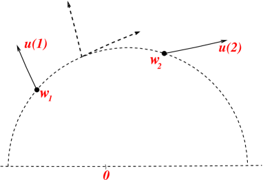
We shall call this paring “extrinsic” as it uses the embedding of the hyperbolic plane into the Minkowski space. It turns out, however, that this pairing is unphysical as it leads to correlation functions of velocity that grow with the distance. Therefore, we use instead an intrinsic way to pair two vectors obtained by taking their scalar product after transporting them by a parallel transport to a common point along the unique geodesic (corresponding to an Euclidiean half-circle centered on the real line in the upper half plane) joining the two attachment points, see Fig. 2.
This leads to the “intrinsic” pairing
| (5.36) |
At equal points, both pairings coincide with the Riemannian scalar product.
6 Harmonic analysis on
The symmetry of functions or vector fields on may be studied with the help of harmonic analysis on , see [23]. In particular, in the space of functions on square-integrable with respect to the volume measure (5.11), the group acts unitarily by the formula
| (6.1) |
The induced infinitesimal action of the Lie algebra is given by the formula and the Laplacian (A.14) by
| (6.2) |
For the reflection in the axis of imaginary acting on by we define the induced action on functions by with the sign for scalar or pseudo-scalar functions. We shall also consider the space of vector fields on with the norm squared , see Eq. (2.1). Group acts an such vector fields by the formula
| (6.3) |
where is the tangent map. In coordinates, if then
| (6.4) |
Action (6.3) preserves . The reflection acts on the vector fields by
| (6.5) |
and also conserves the norm. Both actions map divergenceless vector fields to the vector fields with the same property.
It is convenient to parameterize by the variables , , by writing
| (6.6) |
By acting by on , we may parameterize by the variables (the fractional action of a pure rotation matrix preserves ). In this parametrization, is the hyperbolic distance from . For fixed , the points with different lie on the Euclidean circle in the upper half plane with the center at and with the Euclidean radius . In this parametrization of , the hyperbolic metric and the volume measure become
| (6.7) |
The reflection acts by sending to .
The unitary representation of in may be decomposed into the direct integral of irreducible representations of the even principal series [23]:
| (6.8) |
It is realized by the Fourier transform (in which we substitute to make evident the relation to the flat space decomposition into the polar harmonics that arises in the limit):
| (6.9) |
where
| (6.11) | |||||
are the Legendre functions, and, in particular,
| (6.12) |
Functions satisfy the Legendre equation
| (6.13) |
and the relations
| (6.14) | |||
| (6.15) |
One has the inverse Fourier transform formula:
| (6.16) |
and the Plancherel formula:
| (6.17) |
As in the flat space, the above Fourier transform and its inverse may be generalized to broader classes of functions (and distributions) on .
The even principal series irreducible components of the action (6.1) in , see Eq. (6.8), correspond to fixed . They are spanned by the functions
| (6.18) |
that are eigenfunctions of the hyperbolic Laplacian (6.2) on scalars
| (6.19) | |||||
| (6.20) |
for with the eigenvalue . This follows from the Legendre equation (6.13). The left regular action of on functions (6.18) is given by the formulae:
| (6.21) | |||||
| (6.22) |
As for the reflections,
| (6.23) |
with the sign depending whether we use the scalar or the pseudo-scalar rule. Hence function corresponds in decomposition (6.9) to the Fourier coefficients .
We would like to relate the actions of on functions and on divergenceless vector fields. Every 1-form on satisfying the divergenceless condition may be written as where is a function on , see Eqs. (A.20), (2.13) and (5.24). If corresponds to an incompressible velocity field then is its stream function. The relation between and commutes with the -action. It also commutes with the action of the reflection if is a pseudo-scalar. For the -norm of the divergenceless vector field , one obtains:
| (6.24) |
It follows that the Hilbert space of the divergenceless vector fields with the -norm may be identified with the space of functions with the Sobolev norm (6.24). There is a little catch here [19]. In fact, splits into a direct orthogonal sum of two subspaces
| (6.25) |
by the Hodge decomposition [9]. The square-integrable incompressible vector fields in correspond to stream functions in , whereas the ones in are the harmonic ones such that . The latter may be obtained from harmonic stream functions which do not vanish when tends to the real line, as required for square-integrable functions. By integration by parts, the scalar product (6.24) may be rewritten for as the matrix element , whereas for as the boundary integral over the real axis: . Harmonic vector fields are eliminated if we demand that tend to zero when , as we should do for the well-posedness of the Euler and Navier-Stokes equations on , as mentioned in Appendix B, see also [10, 19]. The decomposition (6.9) induces a decomposition of the non-harmonic subspace of square-integrable (complex) divergenceless vector fields into the irreducible components of the even complementary series of the action of (the harmonic space carries the representation of the discrete series ).
Suppose that the stream functions form a random process with a -invariant distribution and equal-time 2-point function that, consequently, depends only on the hyperbolic distance between the points, see Eq. (5.13),
| (6.26) |
Under the Fourier transform,
| (6.27) |
The positivity of the covariance means that . The equal-time correlation functions of the velocity components are given by the formula
| (6.28) |
For the velocity 2-point function built using the extrinsic paring (5.35), a straightforward although somewhat tedious calculation gives
| (6.29) |
where above and below,
| (6.30) |
coinciding with the action of the Laplacian (6.20) if we view as a function of the distance from . Since the Legendre equation (6.13) reduces for to the relation
| (6.31) |
we obtain the identity
| (6.32) |
where
| (6.33) |
In particular, taking coinciding points, one gets for the mean energy density with the help of (6.14) the spectral integral:
| (6.34) |
We see that the function has the meaning of the energy spectrum. Similarly, for the velocity 2-point function based on the intrinsic pairing (5.36) using the parallel transport, one obtains the expression
| (6.35) |
where
| (6.36) |
The 2-point function of the vorticity is given, in turn, by the formula
| (6.37) | |||||
| (6.38) |
where the second equality results from the expression (6.2) for the hyperbolic Laplacian and the invariance of the 2-point function of . In particular, the mean enstrophy density is
| (6.39) |
i.e. is the enstrophy spectrum.
In fact, we shall be interested in random -covariant velocity processes taking values in incompressible fields and obtained in various limiting regimes. Such processes may not lift to -covariant processes with values in stream functions. If we assume, however, that the velocity equal-time 2-point functions exist and are sufficiently regular ( class is enough) then there exist symmetric functions on of positive type such that Eq. (6.28) holds. Besides,
| (6.40) |
where the dots stand for terms that do not contribute to the velocity 2-point functions that determine function uniquely up to an overall constant. This is shown in Appendix C. The -invariant part might, however, be not of the positive type. Formulae (6.29) and (6.35) still hold in this case.
7 Navier-Stokes equation on the upper half-plane
The Navier-Stokes equation on the upper half-plane takes the form:
| (7.1) | |||
| (7.2) | |||
| (7.3) |
plus its complex conjugate and the incompressibility condition (5.23). As before, we shall suppose that the force is incompressible and non-harmonic, random, white-noise in time, see Eq. (4.4), and that the spatial part of its covariance is
| (7.4) |
The distribution of the force is then invariant under the -transformations and reflections of the vector fields . The mean injection rate
| (7.5) |
is constant in space. A direct calculation shows that
| (7.6) |
Under such forcing and, say, zero initial condition for the velocities, their distribution will be invariant under the -transformations and reflections of .
8 Inverse cascade scenario
We shall assume that the forcing is short-scale, , i.e. that function in Eq. (7.4) vanishes for the arguments not very close to 1 and that viscosity is so small that it does not effect the flow statistics except at distances shorter than . Let us recall that in such situation in the infinite two-dimensional flat space one expects an inverse energy cascade to develop [20, 4]. In terms of the energy spectrum
| (8.1) |
where and , the energy injected around the large modes starting at time flows to smaller building a stationary spectrum for modes , with the decay of for and . This means that asymptotically
| (8.2) |
for large , or, more formally, that in the sense of distributions, where the distribution is defined for small by analytic continuation of from . On the other hand, the enstrophy spectrum becomes stationary
| (8.3) |
and for very long times the enstrophy is dissipated only at short distances (shorter than the injection scale). In the position space,
| (8.4) |
for large times and distances. The inverse cascade means that the scaling function is for small so that
| (8.5) |
for up to terms that vanish when . At long times, the flat-space covariance of the stream function is asymptotically
| (8.6) |
with another constant , where the dots represent terms that vanish for long times and do not contribute the velocity correlation function. When the viscosity is not infinitesimally small, a similar inverse-cascade of energy seems to occur at sufficiently small wavenumbers or long distances, but with the injection rate replaced by its fraction and the rest of the injected energy dissipated at small or moderate distances.
It is reasonable to expect that in the hyperbolic space , the inverse cascade of energy still takes place if for times such that when one can ignore the effects of the curvature. What happens next, is at the moment a matter of a guess. The inverse cascade could stop after the time when it reaches . This is what happens on a sphere of radius where there are no points with distances . After reaching the largest distance, the cascade starts feeding energy into largest-scale flow that eventually changes the spectrum for as well [26]. In the hyperbolic plane, however, there is more and more space available at distances (the circumference of a circle of radius is equal to increasing exponentially with the radius for ). Hence we see no reason for the cascade to stop at . We now explore the scenario of continued flow of energy on to long scales, assuming that at long times the equal-time 2-point correlation function of the stream function takes the form
| (8.7) |
with
| (8.8) |
fixed by the energy injection rate in the limit of vanishing viscosity. From Eqs. (6.29) and (6.35), we obtain then for ”extrinsic” and ”intrinsic” velocity 2-point functions invariant with respect to (that are functions only of time and the hyperbolic distance between the points):
| (8.9) | |||||
| (8.10) |
Such relations should hold for asymptotically long times at distances much longer than the forcing scale . The behavior of and at distances much longer than but much smaller than should approximately be given by Eq. (8.6). We shall try to find in the sequel the asymptotic behavior of those functions at distances much larger than . In particular, we shall see that is very different than the zero wave-number mode proportional to . The spectral consequences of the assumption (8.7) will also be examined.
Actually, similarly to (8.5), we may expect the overall scaling
| (8.11) |
for long times and long distances, see Sec. 10. In what follows, the most important part of our assumption is the finite limit of the scaling function when the first argument is zero, i.e. the existence of . The assumption on the stationarity of the first subleading term is less relevant to the main subject of the paper, which is the nontrivial structure of the growing 2-point function mode .
9 Global flux relation
In the flat space, the inverse cascade pumps the lowest Fourier mode which is constant in space. The stabilization of the spectrum at non-zero translates into the stabilization of the velocity 2nd order structure function. It also permits to extract an exact “flux relation”, that holds at long times and at distances much larger than the forcing scale :
| (9.1) |
Here is a 2-point third-order velocity correlation function, The flux relation, together with the inverse-cascade scenario (8.5), imposes on the position-space energy current across scales a linear growth with the distance:
| (9.2) |
In the present section, we examine analogous implications of the scenario of continuing energy flow to large scales in the hyperbolic plane.
We first consider the velocity 2-point function contracted in the intrinsic way, see Eq. (6.35). For the time derivative of that correlator, we have the expression
| (9.3) |
where
| (9.4) |
is the It term written in terms of the spatial force covariance (7.4). In particular, , see Eq. (7.5). Each term on the right hand side of Eq. (9.3) is a scalar function of two points invariant under the -action on . But for any configuration of two points in there exists an element in that interchanges them. Indeed, any two points may be mapped into any other 2-points with the same value of the cross-ratio , in particular into a pair for such that . Then the action of the rotation matrix exchanges the points. It follows that the first two terms on the right hand side of Eq. (9.3) are equal, i.e. that
| (9.5) | |||
| (9.6) | |||
| (9.7) |
where we introduced a vector field, induced from ,
| (9.8) |
which is the acceleration of a fluid element due to velocity spatial inhomogeneity. We have dropped the contributions from the pressure to the right hand side since the 2-point correlation function of a scalar and a divergenceless vector fields will be shown in a moment to vanish. In complex coordinates,
| (9.9) | |||||
| (9.11) | |||||
| (9.12) | |||||
| (9.13) |
where we have used the identity . The contribution of the first term on the right hand to involves again a correlation function between a scalar and a divergenceless vector fields so it vanishes. Hence
| (9.14) |
for
| (9.15) | |||||
| (9.16) |
where the last equality follows from Eq. (5.13) by a straightforward calculation. We shall denote by the complex conjugate of . These quantities involve equal-time 3-velocity 2-point functions.
The covariance of velocity correlation functions under the transformations and the reflection implies that for ,
| (9.17) | |||
| (9.18) | |||
| (9.19) |
This means that the quantity transforms covariantly under the transformations as a 1-form in its dependence on point and a function in its dependence on point . Eq. (9.14) may be rewritten in the more geometric way as
| (9.20) |
where is the adjoint of the exterior derivative acting on the first variable.
In the inverse cascade scenario, one assumes that the forcing covariance, and hence the function vanishes for and that the limit may be taken. Under those conditions, we infer from Eqs. (9.7) and (9.20) the flux relation
| (9.21) |
holding for . In view of Eq. (8.10), at long times this implies the identity
| (9.22) |
It is a differential equation for the correlation functions and that we shall solve now.
Identities (9.17) and (9.18) imply that there must exist (in general, complex) function such that for
| (9.23) |
This follows from the fact that
| (9.24) |
does not vanish for non-coinciding points and has the same transformation properties under as hence their ratio must be a function of the hyperbolic distance between the points. Relation (9.19) imposes that function must be real. Substitution of relation (9.23) to Eq. (9.22) results in the differential equation
| (9.25) |
whose general solution is
| (9.26) |
The constant has to vanish if the solution for is to be regular at , i.e. at the coinciding points, otherwise would diverge as . We finally infer that
| (9.27) |
Denote by the unit vector tangent at point to the geodesic joining that point to point . Since the geodesics on the upper half plane are half-circles centered at the real line, it is easy to find that
| (9.28) |
and is its complex conjugate. Consider the scalar quantity, that we shall call “intrinsic” energy current,
| (9.29) | |||||
| (9.31) | |||||
| (9.33) |
where the last expression contracts vector with the 1-form at point . Substituting expressions (9.28) and (9.27), we obtain the identity
| (9.34) |
To complete the above arguments, let us prove the vanishing of 2-point correlators between velocity and scalar quantities, used on the way. The correlation functions (either or ) and their complex conjugates also possess the symmetry properties (9.17), (9.18) and (9.19). Hence may be represented as in (9.23) with a real function . We also have the relation
| (9.35) |
due to the incompressibility of . It implies that satisfies the homogeneous version of Eq. (9.25) whose general solution is proportional to . The regularity at the coinciding points of requires that the proportionality constant be zero so that vanishes.
For the extrinsically paired 2-point functions, similar considerations lead to a simpler flux relation
| (9.36) |
with for
| (9.37) |
and complex conjugate . The components of are related by Eq. (9.23) to a function solving now Eq. (9.25) with the right hand side replaced by . Its solution gives
| (9.38) |
The corresponding “extrinsic” energy current
| (9.39) |
10 Scaling
Suppose that we rescale the distances by a constant by changing the metric to . Introduce
| (10.1) | |||||
| (10.2) | |||||
| (10.3) | |||||
| (10.4) |
Then satisfies the Navier-Stokes equation (4.1) for metric with viscosity pressure and forcing if and only if satisfies it for metric with viscosity pressure and forcing . If is a white noise in time with covariance (4.4) then is also white in time with the covariance
| (10.5) |
where . For the dissipation field (4.7) and the mean energy injection rate (4.8), we obtain
| (10.6) |
so that taking assures that they do not change. Let us consider the equal-time correlation of velocities
| (10.7) |
obtained by taking the initial condition . Two basic (essentially tautological) properties of such correlation functions is their diffeomorphism and scaling covariance. The first of those states that for any diffeomorphism of the manifolds
| (10.8) |
for and
| (10.9) | |||
| (10.10) | |||
| (10.11) |
Identity (10.8) is assured by the geometric formulation of the Navier-Stokes equation. On the other hand, the scaling properties of solutions of the Navier-Stokes equation discussed above imply the scaling relation:
| (10.12) |
Let us first recall how these two tautological properties are used in the flat space with and with the spatial forcing covariance . One considers the diffeomorphism for which relation (10.8) reads
| (10.13) |
Using subsequently the scaling property (10.12)
| (10.14) |
one infers that
| (10.15) |
In particular, taking gives:
| (10.16) |
In a flat space, perturbative renormalization-group calculations support the assumption that the limit of the correlation functions exists. The behavior at the forcing scale depends on the dimension. For , experimental and numerical data show that the moments of velocity difference (the velocity structure functions) of all orders except 3 scale with anomalous powers of when and . For , the data suggest that the limits and may be taken for the moments of velocity differences. If this is true, then relation (10.16) implies an asymptotic scaling of the correlation functions in the inverse cascade domain. Note that Eq. (8.4) is a consequence of such a scaling.
Should there be an extension of such conjectures to the curved spaces, in particular, in two-dimensions? The limit of the forcing scale sent to zero still makes sense (in that limit, concentrates on the diagonal with the injection rate kept constant). The main problem is what classes of correlation functions to consider. In a flat space, Galilean invariance suggested considering moments of velocity differences. What is the natural class in the absence of the Galilean invariance of the Navier-Stokes equations? One possible way could be to consider the correlation functions of covariant derivatives of , but is it a good solution?
Let us study more closely the case of the hyperbolic plane. The main problem concerns the behavior of the theory at long distances that we may formulate as the question about the asymptotics at of the correlation functions
| (10.17) |
where , with , are points in Lie algebra . The problem, however, is that the dilation by does not preserve the hyperboloids . If we want that belong to , we have to choose points in a -dependent way so that , but we shall do it so that they tend to limits in the cone when . In this case, the distance between points in general positions will grow with and correlation functions (10.17) will. indeed, test the long-distance behavior of the theory.
Recall that the metric on is induced from the metric on and the forcing covariance is given by Eq. (7.4). The application of identity (10.8) to the diffeomorphism
| (10.18) |
results in the relation
| (10.19) |
Note that . If the forcing covariance is determined by a scalar function from Eq. (7.4) then for points ,
| (10.20) |
where we employed the identities and . Thus the forcing covariance corresponds to the scalar function and to the same energy injection rate as , see Eq. (7.6). Upon relabeling the dependence on the forcing covariance by the function , we obtain from the identities (10.19) and (10.12) with the scaling relation
| (10.21) | |||
| (10.22) |
It seems then that the asymptotic behavior of the right hand side in the limit should be determined by the theory on the limiting space with the vanishing viscosity and the forcing covariance obtained in the limit from . The next section is devoted to a detailed discussion of the ideal hydrodynamics on .
11 Euler equation on
11.1 Limiting geometry
When , the theory on (written e.g. in coordinates of Sec. 6) tends to the one on (written in the radial coordinates), at least for finite times. Let us see what can we tell about the theory in the opposite limit . Due to the scaling properties discussed at the end of the last section, such a limit should provide, at least to some extent, the asymptotic behavior of the theory on at long distances . When , the hyperboloids with approach the (upper light-)cone, see Fig. 1. The theory on should then tend to the one on the cone . In order to parameterize the family of spaces with , it will be convenient to use the coordinates , , with
| (11.1) |
For , these coordinates (with ) parameterize the (upper light-) cone defined by the equation and the inequality . In the variables , the Riemannian metric on is
| (11.2) |
and the metric volume element is
| (11.3) |
When , the metric becomes degenerate with the null radial direction,
| (11.4) |
The metric volume also degenerates, but divided by , has a non-singular limit
| (11.5) |
11.2 Variational principle at
The action functional of Sec. 2 divided by has a limit when
| (11.6) | |||
| (11.7) | |||
| (11.8) | |||
| (11.9) |
By the variational principle, the action (11.6) should give rise to the Euler equation on . Here, we shall study directly the limit when of the Euler equations on in coordinates . The result will be the same (in a slightly different presentation).
In the coordinates , the matrix of inverse metric on is
| (11.10) |
and the non-zero Christoffel symbols are:
| (11.11) |
Hence, in coordinates the Euler equations (2.2) take the form:
| (11.12) | |||
| (11.13) | |||
| (11.14) |
and the incompressibility condition is
| (11.15) |
When , the terms of order from Eq. (11.12) give the condition
| (11.16) |
whereas the terms of order give, with the use of the last equation,
| (11.17) |
where . Eq. (11.14) keeps its form in the limit , whereas the incompressibility condition becomes
| (11.18) |
One can always find a function such that Eq. (11.17) holds, so we may drop it (it does not even appear if we work directly with the variational principle). Hence at , the Euler equation reduces to relations (11.14), (11.16), and (11.18). In terms of the stream function such that
| (11.19) |
and the vorticity , the Euler equation takes the form
| (11.20) |
11.3 Symmetries of the Euler equation on
What are the symmetries of the theory? Since the Lagrangian density (11.9) is independent of time, the time translation invariance gives rise to the conserved currents
| (11.21) | |||
| (11.22) | |||
| (11.23) |
is the energy density. Note that the component of velocity does not contribute to it.
The degenerate metric (11.4) has an infinite-dimensional group of isometries , preserving also the volume form (11.5), given by the transformations
| (11.24) |
where is a diffeomorphism of a circle. In particular, the adjoint action (5.26) of restricted to the cone gives a 3-parameter family of such transformations. The composition of the maps with the transformations (11.24) induces their action on the velocity fields that send to with
| (11.25) | |||
| (11.26) | |||
| (11.27) |
On the other hand, the stream function and the vorticity on transform as scalar functions
| (11.28) |
and it is easy to see that the evolution (11.20) commutes with such transformations. The infinitesimal transformations (11.24) are given by the Killing vector fields
| (11.29) |
In particular, for the infinitesimal transformations induced by matrix ,
| (11.30) |
The Killing vectors (11.29) induce symmetries of the variational problem with the action functional (11.6). They correspond to the conserved currents
| (11.31) | |||
| (11.32) | |||
| (11.33) |
see Eq. (3.20) and (3.21). This can be alternatively presented with purely radial flux: since , we may also take
| (11.34) | |||
| (11.35) |
which shows that at every point there is no exchange of the invariant along the angle, only along the radius.
In Appendix F, we discuss harmonic analysis on , how it arises from that on and how the enhanced symmetry appears in that context.
12 Scaling limit of the theory
In the variables , scaling relation (10.22) may be put into the form
| (12.1) |
if of the indices are equal to and to . The hyperboloids and are taken with their Riemannian metrics that we dropped from the notation. The limit was presumed. In the limit , the correlation function
| (12.2) |
should correspond to the forced correlation functions of the theory on but, as we shall see, the limiting procedure (12.2) is somewhat delicate, at least for some components of the correlation functions. We also should not expect that the limiting correlation functions with forcing respect the symmetry present in the unforced theory at . The aim of the present section is to study these issues in more detail.
12.1 Forcing in the limit
We shall first consider the behavior of the spatial covariance (10.20) on that corresponds to the scalar function . Let us examine how the distance between the points with fixed coordinates and behaves when . According to Eq. (5.6),
| (12.3) | |||||
| (12.4) |
It follows that for ,
| (12.5) |
On the other hand, if then diverges as when . That divergence leads at to the decorrelation of the forcing covariance for different angles if the function in (7.4) is of compact support. For force correlation on given by Eq. (7.4), we obtain the following limiting behavior when :
| (12.6) | |||||
| (12.8) | |||||
| (12.10) |
see Appendix D. Hence the rescaled forcing covariance tends to zero at non-collinear points, but its behavior is very non-uniform when one approaches collinearity. The divergence of the covariance of the radial component of force is consistent with the appearance of the term in the radial component of the Euler equation when . On the other hand, the Euler equation for the angular component of velocity had a finite limit when and so does the covariance of the angular component of force.
It is instructive to inspect how the limit works for the mean energy balance given by the identity
| (12.11) |
where we ignored for the moment the viscous term. The middle term is equal to , with equal contributions from the and terms. How is this reproduced in the theory? Suppose that the latter theory were given by the stochastic equation
| (12.12) |
with white in time with the covariance
i.e. the one obtained in the limit , see Eq. (12.10). If Eq. (12.12) is augmented by the constraint (11.16) and the incompressibility condition (11.18) then we obtain the mean energy balance as follows:
| (12.13) |
The contribution is the Itô term and the second equality results from the identity
| (12.16) | |||||
with the current given by Eqs. (11.22) and (11.23). Under the assumptions, the expectation of the right hand side vanishes (the one of due to the use of the Itô convention). We infer that only half of the energy injection rate is pumped into the mean energy density . The other half has still to be carried by the components forced with the covariance that diverges along the collinear directions.
12.2 Scaling at
For , define
| (12.17) | |||
| (12.18) |
for . Then the fields with “” correspond to the theory with the same forcing as those without “”. It follows that at the velocity correlation functions satisfy
| (12.19) |
if of the indices are equal to and to . This relation would follow from the identity (12.1) but only under the condition that the latter has a limit when , which is not always the case.
Let us consider the 2-point function of the velocity. The only -invariant of two non-colinear points on the cone is
| (12.20) |
where is an arbitrary length scale introduced to render dimensionless. When two points are colinear, i.e. , then their only invariant is . -covariant 2-point functions of the velocity field satisfying the incompressibility condition (11.18) have the form
| (12.22) | |||||
| (12.23) | |||||
| (12.24) |
There are two explicit solutions satisfying scaling (12.19). The first one is proportional to , modulo a logarithmic correction:
| (12.25) |
That leads to
| (12.26) | |||||
| (12.27) | |||||
| (12.28) |
The second sollution is time-independent:
| (12.29) |
leading to
| (12.30) | |||||
| (12.31) | |||||
| (12.32) |
Both solutions preserve the -symmetry but violate the one.
12.3 Velocity 2-point functions
Let us return to the theory on with the equal-time covariance of the stream function
| (12.33) |
where now
| (12.34) |
see Eq. (5.6), and the dots do not contribute to the velocity correlators. The explicit expressions for the rescaled version of the latter in terms of are given in Appendix E. Recall that in Sec. 8 we have postulated the inverse cascade scenario with the long-time behavior of the equal-time covariance of stream function behaving according to Eq. (8.7). Now we may check the consistency of that scenario with the postulated long-time-long-distance asymptotics imposed by the existence of the scaling limit at of the rescaled correlation functions (12.1). Assuming that for large
| (12.35) | |||||
| (12.36) |
together with the first and second derivatives, we infer from the formulae (D.4)-(D.13) of Appendix E that
| (12.37) | |||
| (12.38) | |||
| (12.39) | |||
| (12.40) | |||
| (12.41) | |||
| (12.42) | |||
| (12.43) | |||
| (12.44) | |||
| (12.45) |
for large . Here is given by Eq. (12.20) with . In other words, the scaling limit exists, except for the 2-point function of the radial velocity diverging logarithmically. That divergence could be canceled by a term as in the theory, but appearance of such a term in theory is inconsistent since
| (12.46) |
see Eq. (12.11) and the discussion that follows it. Since the 2-point function of at coinciding points bounds the one at non-coinciding points by the Schwartz inequality, then the latter cannot grow with time faster than linearly (this argument does not work at where does not contribute to the energy balance). The logarithmic divergence with on the right hand side of Eq. (12.39) may rather be related to the collinear divergence of the rescaled covariance of the radial force, see Eq. (12.6). Further checks of that explanation should be performed.
Let us also look at the scaling limit of the velocity 2-point functions at the colinear points with , where
| (12.47) |
We have:
| (12.48) | |||
| (12.49) | |||
| (12.50) |
The term involving behaves as giving no contribution here. The mixed radial-angular velocity correlator vanishes at the collinear configuration, whereas the rescaled radial one is
| (12.51) | |||
| (12.52) | |||
| (12.53) |
The right hand side diverges when , confirming the singular character of the radial velocity correlators in this limit.
In all, the above analysis shows the consistency of the scenario (8.7) with the asymptotic behavior of the modes and for large given by relations (12.35) and (12.36) and their first two derivatives, in particular, of the asymptotic equalities
| (12.54) |
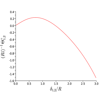
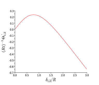
If we extrapolate this asymptotic behavior to values of then relation (8.8) fixes the value of to whereas relation (12.13) for the scaling limit (12.45) of the correlation function fixes to the value . With such an extrapolation, the growing-in-time contributions to the ”intrinsic” and ”extrinsic” invariant velocity 2-point functions are given by the relations
| (12.55) | |||||
| (12.56) |
for . Figures 4 and 4 show the dependence of the respective expressions on .
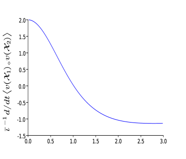
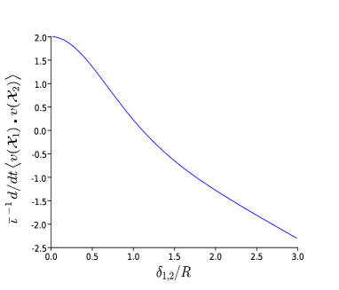
The time derivatives of both invariant 2-point functions are equal to at the coinciding points, in accordance with the energy balance, and stay close to that value, to which they would be locked in the flat space, at . They change sign around showing that velocities become anti-correlated at the distances exceeding the curvature radius. Continuing growth with the distance of the absolute value of the extrinsic function shows that this is not the proper object to describe velocity correlations at different points. We therefore focus on physically more meaningful intrinsic 2-point function, which tends to the constant at large distances. That means that, when compared using the parallel transport along geodesics, the velocities stay anti-correlated at long times and long distances by half of the value at coinciding points. Most probably, that behavior of the correlation function may be interpreted as follows. Our energy condensing mode is not a coherent motion, but a correlation function contribution, i.e. it is built of separate pieces of flow. Those look like a uniform flow only at distances shorter than the radius of curvature. Indeed, inverse cascade in a flat space produces ever-increasing pieces of almost uniform velocity, which locally look like jets. However, when the transversal extent of a jet overgrows the curvature radius , the jet splits into two. Anti-correlation at larger distances means that they are circular motions. The fact that anti-correlation persists to arbitrary large (ever-increasing with time) scale means that there are vortex rings with arbitrary large radius, but the fact that the positive correlation is only until means that those vortices are actually narrow rings with the width of order . Incidentally, the value of the correlation at large distances being half of the value at zero follows from the picture of a jet (at distances smaller than ) splitting into two vortices. The fact that we do not grow ever-increasing pieces of a uniform flow is likely related to the absence of Galilean invariance. Why curved space favors rings is unclear. It would be interesting to look at concrete examples of such flows on the hyperbolic plane.
Similarly, Figures 6 and 6 show the dependence on of the ”intrinsic” and ”extrinsic” energy current of Eqs. (9.34) and (9.39) given, under the extrapolation assumption, by the expressions
| (12.57) | |||||
| (12.58) |
Both expressions behave as for distances , which is the flat space behavior. For larger distances both reach a maximum and eventually turn negative. The absolute value of the intrinsic current increases then exponentially in at long distances whereas that of the extrinsic current behaves asymptotically as . The behavior of the intrinsic (i.e. physically meaningful) energy current suggests that at large distances it is proportional (with a logarithmic accuracy) to the circumference rather than to the radius . To interpret it, recall that the flux through the scale is the energy density at that scale divided by the turn-over time , and the energy flux constancy predicts . Identifying with we see that must be taken as the circumference rather than the radius in the relation for the turnover time. That probably makes sense since what mostly contributes to the velocity difference between two points (and the energy at this scale) is an eddy, i.e. a flow along circumference having these two points at opposite ends.
What is the meaning of this saturation of current at intermediate distances? In a flat space, divergence of the current is the energy transfer rate which is a scale-independent constant for a cascade. In our case, we see that the transfer rate decreases with increase of the distance and changes sign (when current saturates) at a distance comparable to the radius of curvature. This seems consistent with the non-cascade behavior at longer distances, namely the growth of the energy condensing autocorrelation mode carried by large-scale motions.
The contribution of the stationary mode to both invariant 2-point functions is expected to have the flat space behavior for whereas for large distances its behavior should be leading to an exponential decrease when .
What can we infer about the energy spectrum from the behavior of and at large ? Suppose that and behave asymptotically as in Eqs. (12.35) and (12.36) up to a sum of negative, possibly fractional, powers of . In particular, both modes are very different than the zero wavenumber mode that decreases as , see (F.14). We show in Appendix G that under these assumptions, the contributions of and to the energy spectrum are analytic around the positive real axis including , in contrast with the flat space behavior where and . In particular, the stationary autocorrelation mode then contains finite energy (per unit area), unlike in the flat space case.
13 Conclusions
We considered an inverse cascade scenario for the two-dimensional turbulence in the hyperbolic plane described by the Navier-Stokes equation with a random Gaussian white-in time forcing operating on scales much shorter than the curvature radius . The main focus was on the possible structure of the mode of the equal-time 2-point velocity function growing linearly in time. On distances much smaller than the curvature radius, where one can ignore the curvature effects, such a mode should behave similarly to the energy condensing constant mode in a flat space. Long-distance long-time scaling limit of the theory on hyperbolic plane lives on the conical surface. By analyzing such theory, we have found the long-distance behavior of the energy condensing mode and of the energy current across scales. Their behavior indicates that the energy transfer on scales longer than loses the cascade character where the energy flux is constant across scales and the spectrum stabilizes up to smaller and smaller wave numbers. Instead, the spectral density in all scales eventually grows linearly in time and the energy current across scales reaches a maximum around the curvature radius distance. The analytic results seem to indicate that the energy is cumulated in ring-like vortices of arbitrary diameter but of width of order . While these results have not brought any direct progress in understanding the conformal-invariant sector of the inverse cascade visible in the statistics of the zero-vorticity lines, yet we exhibited on the way the -symmetry of the unforced Euler equation in the asymptotic geometry at infinity of the hyperbolic plane. This infinite-dimensional conformal symmetry in one dimension appears, however, to be broken by the forcing. The analysis that we performed here was limited to few consistency checks on and few implications of the inverse-cascade scenario assumed for the hyperbolic-plane turbulence. It calls for numerical simulations that could confirm or refute the picture put forward here. Such simulations would have to adapt the numerical schemes for flat-space two-dimensional turbulence to the context of the hyperbolic geometry, which is not a trivial task. The problem of turbulence in the hyperbolic plane might seem somewhat academic as such geometry is not realized by surfaces in three-dimensional Euclidean space [17]. Nevertheless, the basic results about the influence of the negative curvature on the behavior of the cascade at distances longer than the curvature radius may have some bearing on the fate of the inverse cascade in soap bubbles and films that form surfaces with negative curvature. Measuring such curvature effects in the soap film turbulence [18] would be a challenge for experimentalists.
14 Appendices
Appendix A Some notions of Riemannian geometry
Let be a -dimensional oriented manifold equipped with a Riemannian metric . Such a metric may be used to lower the indices of the contravariant tensor fields, e.g. . One has , where is the matrix inverse to . The metric together with the orientation induces the volume form , where is the shorthand notation for . A Riemannian metric induces the Levi-Civita connection acting on tensor fields by
| (A.1) | |||
| (A.2) |
where are given by the Christoffel symbols
| (A.3) |
For the Levi-Civita connection, the covariant derivatives of the tensors and vanish so that commutes with the raising and lowering of indices. The Riemann curvature tensor is defined by the formula
| (A.4) |
and Ricci tensor by
| (A.5) |
The scalar curvature is . The totally antisymmetric tensors may be identified with the differential forms by the correspondence
| (A.6) |
The exterior derivative in terms of this identification is given by the formula
| (A.7) | |||||
| (A.8) |
The Hodge star on -forms is defined by
| (A.9) |
It satisfies . The scalar product of -forms is given by
| (A.10) |
The (formal) adjoint of the exterior derivative mapping -forms to -forms is the operator
| (A.11) |
mapping -forms to -forms. In terms of the tensor components,
| (A.12) |
The (negative) Laplace-Beltrami operator is
| (A.13) |
In the action on functions, it gives
| (A.14) |
The Laplace-Beltrami operator act also on vector fields by the formula
| (A.15) |
where is the 1-form represented by associated to the vector field represented by . We also need the Lie derivative of tensors w.r.t. vector fields given by the formulae
| (A.16) | |||
| (A.17) | |||
| (A.18) |
in the action on the vector fields and 1-forms, respectively, and by the Leibniz rule on higher tensors. In particular, the vector fields are called Killing vectors if annihilate the metric tensor :
| (A.19) |
We also consider divergenceless vector fields defined by the condition . In coordinates, the condition is equivalent to the conditions or . Yet another form of this condition is the requirement that . Locally, every 1-form satisfying such condition can be written via -form :
| (A.20) |
Appendix B Variation principle for Euler equation
It will be convenient to perform the extremization over all diffeomorphisms imposing the volume-preservation constraint by adding to the action a term
| (B.1) |
with a Lagrange multiplier . For the variation of at volume-preserving , we obtain333field theorists will notice a similarity of the following calculation to those in nonlinear sigma models:
| (B.2) | |||
| (B.3) | |||
| (B.4) | |||
| (B.5) | |||
| (B.6) | |||
| (B.7) | |||
| (B.8) | |||
| (B.9) |
where and is the covariant derivative with respect to the Levi-Civita connection. On the other hand, the variation of is given by
| (B.10) | |||
| (B.11) | |||
| (B.12) | |||
| (B.13) | |||
| (B.14) | |||
| (B.15) | |||
| (B.16) | |||
| (B.17) | |||
| (B.18) | |||
| (B.19) | |||
| (B.20) |
where we have introduced the pressure by the formula
| (B.21) |
Integrating by parts in the last term, we finally obtain
| (B.22) | |||
| (B.23) | |||
| (B.24) |
Equating to zero the variation for , we obtain the (generalized) Euler equation (2.2) together with the volume-preserving condition on which, in terms of the velocity is the incompressibility condition (2.3). On noncompact manifolds, these should be accompanied by the decay conditions at infinity that assure that the integrations by parts above may be performed and eliminate the solutions with and arbitrary -dependence (solving also the unforced Navier-Stokes equations on Einstein manifolds, see [10, 19]).
Appendix C Velocity covariance in terms of stream functions
is a contractible space. On the other hand, due to incompressibility of velocity, the equal-time 2-point function is a closed 1-form in its dependence on each of the two points. We may then obtain a stream-function correlator satisfying Eq. (6.28) by integrating in each variable from a fixed point of to and , respectively. Function obtained this way is symmetric and of positive type, but it depends on the choice of the initial point of integration. As a result, the -covariance of the velocity 2-point function does not imply the invariance of . However, for , the function
| (C.1) |
is annihilated by the product of exterior derivatives in and . It has then to be of the form where, by symmetry, we may take . Definition (C.1) implies the cocycle condition
| (C.2) |
Taking, in particular, corresponding to and , which is the stabilizer subgroup of , we obtain
| (C.3) |
Taking also , we infer that is an additive function of , so it must be equal to zero when restricted to such . Consequently, for general , one has , so that defines a function on (vanishing at ) and it determines by the formula
| (C.4) |
following from the cocycle condition (C.2). This, in fact, provides a general solution of this condition if we consider arbitrary functions on . Note that the symmetric function satisfies the relation , hence it depends only on the hyperbolic distance . It defines the same velocity correlators if used in formula (6.28) instead of . If is another such functions, then
| (C.5) |
for some function . The -covariance of and implies then that
| (C.6) |
but for each there is such that and we infer that so that function is constant.
Appendix D Forcing covariance on
Appendix E Rescaled velocity 2-point functions on
Assuming the form (12.33) of the 2-point correlator of the stream function on , the rescaled version of the velocity 2-point functions given by Eq. (6.28) may be written in the form:
| (E.1) | |||
| (E.2) | |||
| (E.3) | |||
| (E.4) | |||
| (E.5) | |||
| (E.6) | |||
| (E.7) | |||
| (E.8) | |||
| (E.9) | |||
| (E.10) | |||
| (E.11) | |||
| (E.12) | |||
| (E.13) | |||
| (E.14) | |||
| (E.15) |
where is given by the right hand side of Eq. (12.34) with replaced by . The above expressions should be compared to Eqs. (12.22), (12.23) and (12.24) for the velocity correlators on .
Appendix F Harmonic analysis on in the limit
To study the harmonic analysis on in the limit , we rewrite it using the coordinates . The harmonic analysis in space is realized by the formulae that combine the Gel’fand-Graev transformation from functions on the hyperboloid to functions on the cone
| (F.1) |
with the Fourier transform in the angular direction and Mellin transform in the radial one [23]. In the coordinates it is given by the relations:
| (F.3) | |||||
| (F.4) | |||||
| (F.5) | |||||
| (F.8) | |||||
| (F.9) | |||||
| (F.13) | |||||
which reproduce Eqs. (6.9), (6.16) and (6.17) upon setting .
To study the limit, we use the asymptotic expansion from [16] holding for large positive :
| (F.14) |
Substituting this to Eq. (F.5) and using the relation , we obtain
| (F.16) | |||||
| (F.18) |
where we have set
| (F.19) |
Hence, the limiting decomposition at of functions on the cone is given by the Mellin transform in combined with the Fourier transform in the angular variable :
| (F.20) | |||
| (F.21) | |||
| (F.22) | |||
| (F.23) | |||
| (F.24) |
Action (11.24) of on induces the unitary action of that infinite-dimensional group in the space of functions on square-integrable with respect to the volume measure , defined by the formula
| (F.25) |
Note that this action commutes with the Laplacian . The functions are eigenvectors of corresponding to the eigenvalue . The decomposition (F.20) realizes the decomposition of into the spectral eigenspaces of and, at the same time, the decomposition of the unitary representation of in into the irreducible components:
| (F.26) |
Unlike for , where only appeared in the decomposition (6.8), now and give rise to inequivalent representations.
Appendix G Real analyticity of the spectrum
Spectrum is related to the stream function correlator by the Fourier transform on (6.27) and Eq. (6.33) which imply the inverse transform relation
| (G.1) |
where the integral has to be interpreted in the appropriate sense (by analytic continuation) since, for large , , see Eqs. (F.14). Let us split the integration on the right hand side of (G.1) into the one from 1 to 2 and the rest. The first integral gives an entire function of , as is easily seen from Eq. (6.12), and it contributes to a term or less for small . For the other integral, we shall use the expression
| (G.2) |
for . Expanding the hypergeometric functions into a power series in , we see that only the contribution
| (G.3) |
of the leading term into the integral needs a special treatment. Using the asymptotic expansion for rewritten in terms of variable , we see that the integral (G.3) contributes few simple poles and a function analytic in in a neighborhood of the real axis. The pole at zero appears only if the power occurs in the large expansion of . The other terms of the expansion of the hypergeometric functions contribute absolutely convergent integrals so that
| (G.4) |
is again analytic in in a neighborhood of the real axis. The prefactors in Eq. (G.2) are meromorphic in in such a region with a simple pole at . Eq. (G.1) implies than that the contribution of is analytic around . As for the contribution to , a presence of the term in its asymptotic expansion could leave us with a pole at of up to the second order (due to up to two derivatives over used to produced the logarithmic terms of ), but such pole would be incompatible with the finiteness of the energy density at finite times. Hence the contribution of to the spectrum should also be analytic around .
References
- [1] A. Arneodo et al.: Structure functions in turbulence, in various flow configurations, at Reynolds number between 30 and 5000, using extended self-similarity, Europhys. Lett. 34 (1996), 411-416
- [2] V. I. Arnold: Sur la géométrie différentielle des groupes de Lie de dimension infinie et ses applications à l’hydrodynamique des fluides parfaits, Ann. Inst. Fourier (Grenoble) 16 (1966), 319-361
- [3] V. I. Arnold, B. Khesin: Topological Methods in Hydrodynamics, Appl. Math. Scien. vol. 125, Springer, New York
- [4] G. K. Batchelor: Computation of the energy spectrum in homogeneous two-dimensional turbulence, Phys. Fluids Suppl. II 12 (1969), 233-239
- [5] D. Bernard, G. Boffetta, A. Celani, G. Falkovich: Conformal invariance in two-dimensional turbulence, Nature Physics 2 (2006), 124-128
- [6] D. Bernard, G. Boffetta, A. Celani, G. Falkovich: Inverse turbulent cascades and conformally invariant curves, Phys. Rev. Lett. 98 (2007), 024501
- [7] G. Boffetta, A. Celani and M. Vergassola: Inverse cascade in two-dimensional turbulence: deviations from Gaussianity, Phys. Rev. E 61 (2000), R29R32
- [8] G. Boffetta, S. Musacchio: Evidence for the double cascade scenario in two dimensional turbulence, Phys. Rev. E 82 (2010), 016307(1-5)
- [9] G. Carron: harmonics forms on non-compact manifolds, arXiv:0704.3194 [math.DG]
- [10] C. H. Chan, M. Czubak: Non-uniqueness of the Leray-Hopf solutions in the hyperbolic setting, Dynamics of PDE 10 (2013), 43-77
- [11] D. G. Ebin, J. Marsden: Groups of diffeomorphisms and the motion of an incompressible fluid, Ann. of Math. 92 (1970), 102-163
- [12] G. Falkovich: Fluid Mechanics, a short course for physicists, Cambridge Univ. Press, Cambridge 2011
- [13] G. Falkovich, K. Gawedzki, M. Vergassola: Particles and fields in fluid turbulence, Rev. Mod. Phys. 73 (2001), 913-975
- [14] U. Frisch: Turbulence: the Legacy of A. N. Kolmogorov, Cambridge Univ. Press, Cambridge 1995
- [15] U. Frisch, B. Villone: Cauchy’s almost forgotten Lagrangian formulation of the Euler equation for 3D incompressible flow, arXiv:1402.4957 [math.HO]
- [16] I.S. Gradshteyn, I.M. Ryzhik: Table of Integrals, Series, and Products, Seventh Edition, Academic Press, Amsterdam 2007
- [17] D. Hilbert, Über Flächen von constanter Gaußscher Krümmung, Trans. Amer. Math. Soc. 2 (1901), 87–99
- [18] H. Kellay, W. I. Goldburg: Two-dimensional turbulence: a review of some recent experiments, Rep. Prog. Phys. 65 (2002), 845-894
- [19] B. Khesin, G. Misiolek: The Euler and Navier-Stokes equations on the hyperbolic plane, Proc. Nat. Acad. Sci. 109 (2012), 18324-18326
- [20] R. H. Kraichnan: Inertial ranges in two-dimensional turbulence, Phys. Fluids 10 (1967), 1417-1423
- [21] S. Kuksin, A. Shirikyan, Mathematics of Two-Dimensional Turbulence, Cambridge Univ. Press, Cambridge 2012
- [22] J. Paret and P. Tabeling: Intermittency in the 2D inverse cascade of energy: experimental observations, Phys. Fluids 10 (1998), 3126-3136
- [23] N. Ja. Vilenkin: Special Functions and the Theory of Group Representations, Transl. Math. Monograph, 21, Amer. Math. Soc. 1968
- [24] M. J. Vishik, A. V. Fursikov: Mathematical Problems of Statistical Hydrodynamics, Kluwer Academic Publishers, Dordrecht 1988
- [25] M. Vucelja, G. Falkovich, K. S. Turitsyn: Fractal iso-contours of passive scalar in two-dimensional smooth random flows, J. Stat. Phys. 147 (2012), 424-435
- [26] H Xia, M Shats, G Falkovich: Spectrally condensed turbulence in thin layers, Phys. Fluids 21 (2009), 125101